Mathematical modelling of transport phenomena in compressible multicomponent flows

Abstract

The present article proposes a diffuse interface model for compressible multicomponent flows with transport phenomena of mass, momentum and energy (i.e., mass diffusion, viscous dissipation and heat conduction). The model is reduced from the seven-equation Baer-Nuziato type model with asymptotic analysis in the limit of instantaneous mechanical relaxations. The main difference between the present model and the Kapila’s five-equation model consists in that different time scales for pressure and velocity relaxations are assumed, the former being much smaller than the latter. Thanks to this assumption, the velocity disequilibrium is retained to model the mass diffusion process. Aided by the diffusion laws, the final model still formally consists of five equations. The proposed model satisfy two desirable properties : (1) it respects the laws of thermodynamics, (2) it is free of the spurious oscillation problem in the vicinity of the diffused interface zone. For solution of the model governing equations, we implement the fractional step method to split the model into five physical steps: the hydrodynamic step, the viscous step, the heat transfer step, the heat conduction step and the mass diffusion step. The split governing equations for the hydrodynamic step formally coincide with the Kapila’s five equation model and are solved with the Godunov finite volume method. The mass diffusion, viscous dissipation and heat conduction processes contribute parabolic partial differential equations that are solved with the Chebyshev method of local iterations. Numerical results show that the proposed model maintains pressure, velocity and temperature equilibrium near the diffused interface. Convergence tests demonstrate that the numerical methods achieve second order in space and time. The proposed model and numerical methods are applied to simulate the laser-driven RM instability problem in inertial confinement fusion, good agreement with experimental results are observed.

1 Introduction

Compressible multicomponent flows are of significance to many applications, such as the inertial confinement fusion (ICF), the explosion of core-collapse supernova, underwater explosion (UNDEX) and so forth. These physical processes include Rayleigh-Taylor (RT) and Richtmyer-Meshkov (RM) hydrodynamic instabilities that rapidly develop in the presence of small initial perturbations. Up to now, understanding the development of these nonlinear instabilities still heavily relies on numerical simulations. The present research is motivated by the need to simulate the laser-driven plasma instability developed at the interface between dissimilar materials within ICF capsules. In such applications, the transport phenomena (of mass, momentum and energy) accompanying the hydrodynamic process play significant role. First of all, the laser energy deposited in the plasma is transported through the heat conduction process. Moreover, at small spatial scales the effect of viscous dissipation and the mass diffusion begin to impact the instability growth [1]. Numerically, the transport process is vital for achieving a grid-converged DNS (Direct Numerical Simulation) [2].

To correctly simulate the dissipative processes in multicomponent flows, the governing model should satisfy two important criteria, i.e., physically admissibility and numerical consistency. The former stipulates that the model should respect the first and second law of thermodynamics. The latter dictates that the closure relations and numerics do not cause non-physical spurious oscillations near the material interface. Several works in the literature have attempted in this direction [3, 4]. The present work is performed in the framework of the diffuse interface model (DIM). We aim to incorporate various dissipative transport phenomena (including mass diffusion, viscous dissipation and heat conduction) into this framework with the above two criteria being maintained.

The fully conservative four-equation DIM (i.e., Euler equation supplemented with one conservation equation for the partial density) is notorious for triggering spurious oscillations in pressure and velocity (at the hydrodynamic stage) when solved with the Godunov finite volume method (FVM). Analysis works on this phenomenon have been performed both physically and numerically [5, 6, 7]. In this model there exists only one temperature and one pressure, implicitly assuming that the components are in thermal and mechanical equilibrium. This assumption is commonly used for combustion and boiling problems, however, it maybe too strong to be valid for interface problems. Pressure and temperature disequilibria are diminished by compaction (pressure relaxation) and heat transfer (temperature relaxation) between components, respectively. However, these two processes may take place at very different time scales. For example, for the deflagration-to-detonation transition (DDT) in granular materials, the characteristic time scales for pressure relaxation and temperature relaxation are 0.03$\mu s$ and 18000$\mu s$ after sufficient combustion [8], respectively. It is evident that forcing thermodynamical equilibrium to be reached at the same time scale may lead to physical inconsistency.

To understand the temperature closure relations within the computational cell, let us look at the resolved interface problem in in-miscible multicomponent flows (Figure 1). According to the Rankine-Hugoniot relation, the jump conditions across the interface (the line $C$ in Figure 1) along its normal direction read:

$$\llbracket\rho Y_{1}(u_{n}-\mathcal{U})\rrbracket=0,$$ (1a)

$$\llbracket\rho Y_{2}(u_{n}-\mathcal{U})\rrbracket=0,$$ (1b)

$$\llbracket p+\rho\boldsymbol{u}(u_{n}-\mathcal{U})\rrbracket=0,$$ (1c)

$$\llbracket(u_{n}-\mathcal{U})\left(\rho e+\frac{\rho|\boldsymbol{u}-\mathcal{U}\boldsymbol{n}|^{2}}{2}+p\right)+J_{qn}\rrbracket=0,$$ (1d)

where $\rho$, $Y_{k}$, $e$ are the mixture density, the mass fraction of component $k$, and the mixture internal energy. $u_{n}$, $\mathcal{U}$, $J_{qn}$ are normal components to the interface $C$ of the particle velocity $\boldsymbol{u}$, the interface velocity, and the heat flux, respectively. The operator $\llbracket\phi\rrbracket=\phi_{2}-\phi_{1}$ with the subscripts $1/2$ denoting the variables on the left/right of the discontinuity, or the states of the 1/2-fluid.

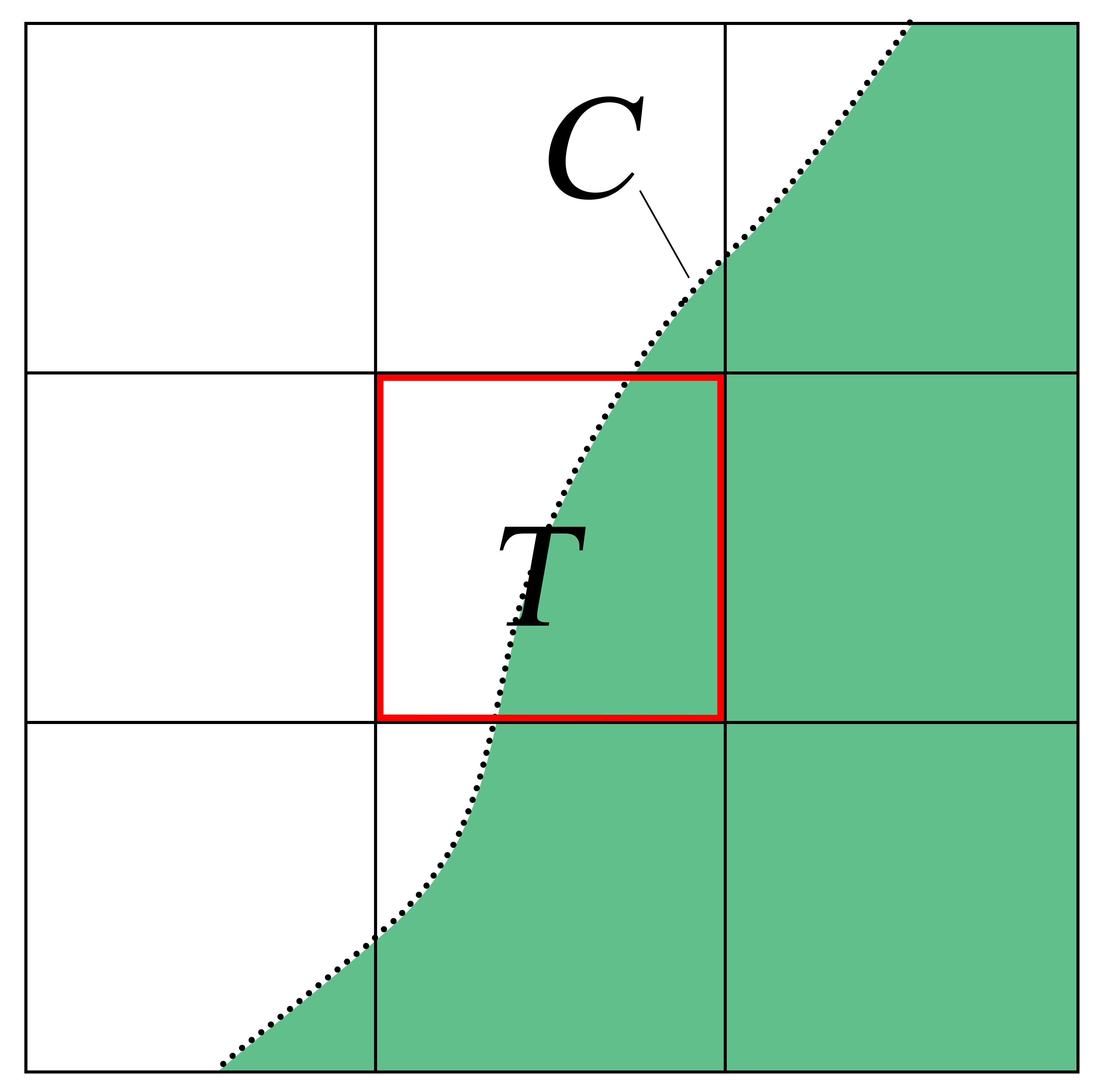
(a) Equilibrium temperatures

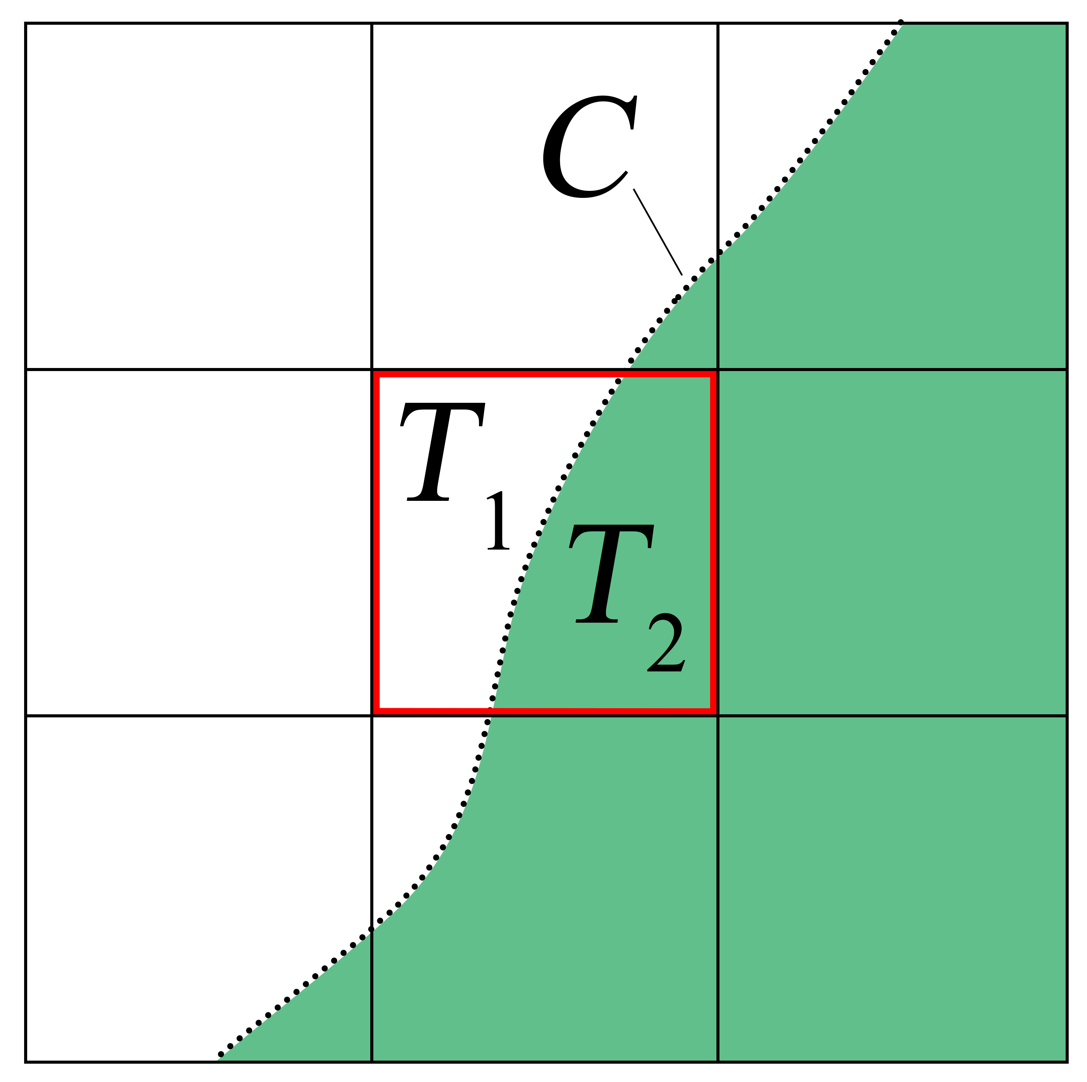
(b) Disequilibrium temperatures

(c) Miscible interface

Figure 1: Interfaces on computational grid.

The interface represents a contact discontinuity, across which velocity is continuous, i.e., $u_{n1}=u_{n2}=\mathcal{U}$. From eqs. 1c and 1d follows $\llbracket p\rrbracket=0$ and $\llbracket J_{qn}\rrbracket=0$, respectively. With the Fourier’s heat flux, the latter can be expressed as:

$$\left(\lambda_{1}\nabla{T_{1}}\right)\boldsymbol{\cdot}\boldsymbol{n}=\left(\lambda_{2}\nabla{T_{2}}\right)\boldsymbol{\cdot}\boldsymbol{n},$$ (2)

where $\lambda_{k}$ is the heat conduction coefficient of component $k$.

In the framework of the DIM, the material interface contained within a computational cell is not tracked and the properties of fluids are diffused within the interfacial zone. Thermal conductivity imposes temperature continuity across the interface. If the model is equipped with only one temperature, then the two materials inside a computational cell share the same temperature (i.e., $T_{1}=T_{2}=T$, Figure 1a), which maybe inconsistent with eq. 2. This inconsistency results in numerical errors of FVM or physical inconsistency in the vicinity of the interface. In fact, the equilibrium temperature assumption means that temperature relaxation rate is infinitely large so that phase temperature equilibrium is reached instantaneously. This assumption deprives the model of the ability to deal with physically finite relaxation rates.

To get rid of the above-mentioned temperature inconsistency, we turn to the temperature-disequilibrium models. In such models each cell state is characterized with temperatures for each component (Figure 1b), and thus the temperature equilibrium is not enforced. One representative of such models is the Baer-Nuziato (BN) model [9] and its variant [7] for compressible multiphase flows. Formally, the BN model include balance equations for the partial density, the phase momentum and the phase total energy and is argumented with an evolution equation for volume fraction. The latter is vital for maintaining the free-of-oscillation property at the interface. In this model, each component is described with a full set of parameters (density, velocity, pressure and temperature) and governed by the single-phase Navier-Stokes (NS) equations away from the interface. The interactions between components only happen in the neighbourhood of the interface. These interactions include the kinetic, mechanical and thermal relaxations that strive to erase the disequilibria in velocity, pressure and temperature. The temperature equilibrium (imposed in one-temperature DIMs) is reached only after the complete temperature relaxation. The characteristic relaxation rates depend on particular physical problems. The model is unconditionally hyperbolic and respect the laws of thermodynamics. Moreover, in DIM the phase temperatures exist all through the computational domain since even the pure fluid is approximated as a fluid with negligible amount of other components. The disequilibrium temperature closure in each computational cell does not introduce inconsistency with the heat flux jump conditions.

Although the BN model is physically complete, it consists of complicated wave structure and stiff relaxation processes, making its numerical implementation quite cumbersome. For many application scenarios, the model can be simplified to a large extent. For example, for the DDT process, Kapila et al. have derived two reduced models in the limit of instantaneous mechanical relaxations [8]. The first model is obtained in the limit of instantaneous velocity relaxation and consists of six equations. Only one equilibrium velocity exists in this model. This formulation is used for solving Kapila’s five-equation model in [10] for improving robustness. The second is the well-known five-equation model and derived in the limit that both pressure and velocity relaxation rates approach infinity (Figure 2).

Figure 2: Schematic of reduced models.

Most current DIM works in literature focus on the resolved interface problem, however, the components maybe miscible and penetrate into each other (Figure 1c). Under such circumstances, there is no longer a definite sharp discontinuous material interface, but a a physically diffused zone with finite thickness. This diffused zone develops as a result of mass diffusion and enthalpy diffusion. The significance of the latter to maintain the thermodynamical consistency has been demonstrated in [4]. In fact, the enthalpy diffusion appear as a result of replacing the phase velocities with the mass-weighted one for any multi-velocity model, including the BN model.

From a microscopic point of view, mass diffusion is the result of molecular random motions, which drives the molecular distribution toward uniformity. In the macroscopic continuum mechanics where each spatial element contains enormous number of molecules, the mass diffusion flux is characterized by the velocity difference between different species. Thus, the one-velocity models of Kapila is incapable of modelling this process. When the mass diffusion effect is strong, the velocity relaxation time scale is comparable to that of the problem considered and the assumption of instantaneous velocity relaxation is inappropriate. Therefore, to model the mass diffusion, we have to retain the velocity disequilibrium and then close it with diffusion laws (Figure 2), which is one of the major contributions of the present paper.

The reduction procedures in [11, 12] assume the same relaxation time scale for velocity and pressure. This approach inevitably leads to velocity-equilibrium models where no mass diffusion sustains. Instead, weighing simplicity and thermodynamic consistency, we assume different time scales for the velocity and pressure. The pressure relaxation time scale is much smaller than that of the velocity. Such an assumption is in fact supported many physics, for example, see [8, 13, 14, 15]. With this assumption and the diffusion laws, the seven-equation BN model can be reduced to a five-equation one without losing the ability to model the mass diffusion process.

In reducing the velocity-disequilibrium model, the second order term of the velocity relaxation time is abandoned. The finally obtained model formally contains one velocity. However, this velocity is the mass-weighted mixture velocity rather than the equilibrium velocity in Kapila’s model. The component velocities can be derived by invoking diffusion laws. The finally obtained model satisfy both of the two criteria (physical admissibility and numerical consistency) proposed above.

We propose numerical methods for solving the model with the fractional step method. In numerical implementation, the model is split into five physical parts, i.e., the hydrodynamic part, the viscous part, the temperature relaxation part, the heat conduction part and the mass diffusion part. The first part formally coincides with the original Kapila’s formulation, however, the velocity owns different physical meanings (as discussed in the last paragraph). Various Godunov FVM methods in literature (for example, see [16, 12, 17, 18]) can be used to solve the governing equations for the hydrodynamic part. In the first two parts the component temperatures are in disequilibrium. The temperature relaxation takes place at a much larger time scale and solved separately after these parts. The diffusion processes (including viscous dissipation, heat conduction and mass diffusion processes) are governed by parabolic PDEs, that are solved with the locally iterative method based on the Chebyshev parameters [19, 20]. The heat conduction and mass diffusion equations are solved maintaining the temperature equilibrium, i.e., assuming an instantaneous temperature relaxation. Note that finite temperature relaxation can also be considered straightforwardly.

The rest of the present paper is organized as follows. In Section 2 we derive the reduced model by performing the asymptotic analysis on the BN-type model in the limit of instantaneous mechanical relaxations. In Section 3 we develop numerical methods for solving the proposed model. In Section 4 we present numerical results for several multicomponent problems with diffusions and apply the model and numerical methods to the laser ablation problem in the field of ICF.

2 Model formulation

2.1 The BN-type seven-equation model

The starting point of the following model formulation is the complete BN-type seven-equation model [9, 7, 21, 12], which can be derived by using the averaging procedure of [22]. It reads:

$$\frac{\partial{\alpha_{k}\rho_{k}}}{\partial{t}}+\nabla\boldsymbol{\cdot}(\alpha_{k}\rho_{k}\boldsymbol{u}_{k})=0,$$ (3a)

$$\frac{\partial{\alpha_{k}\rho_{k}\boldsymbol{u}_{k}}}{\partial{t}}+\nabla\boldsymbol{\cdot}\left(\alpha_{k}\rho_{k}\boldsymbol{u}_{k}\boldsymbol{\otimes}\boldsymbol{u}_{k}-\alpha_{k}\overline{\overline{T}}_{k}\right)=-\overline{\overline{T}}_{I}\boldsymbol{\cdot}\nabla{\alpha_{k}}+\mathcal{M}_{k},$$ (3b)

$$\frac{\partial{\alpha_{k}\rho_{k}E_{k}}}{\partial{t}}+\nabla\boldsymbol{\cdot}\left(\alpha_{k}\rho_{k}E_{k}\boldsymbol{u}_{k}-\alpha_{k}\overline{\overline{T}}_{k}\boldsymbol{\cdot}\boldsymbol{u}_{k}\right)=-\boldsymbol{u}_{I}\boldsymbol{\cdot}\left(\overline{\overline{T}}_{I}\boldsymbol{\cdot}\nabla{\alpha_{k}}\right)+\boldsymbol{u}_{I}\mathcal{M}_{k}-p_{I}\mathcal{F}_{k}+\mathcal{Q}_{k}+q_{k}+\mathcal{I}_{k},$$ (3c)

$$\frac{\partial{\alpha_{k}}}{\partial{t}}+\boldsymbol{u}_{I}\boldsymbol{\cdot}\nabla\alpha_{k}=\mathcal{F}_{k},$$ (3d)

where the notations used are standard: $\alpha_{k},\;\rho_{k},\;\boldsymbol{u}_{k},\;p_{k},\;\overline{\overline{T}}_{k},\;E_{k}$ are the volume fraction, phase density, velocity, pressure, stress tensor, and total energy of phase $k$. For the sake of clarity we constrict our discussions within the scope of two-phase flows, $k=1,2$. The phase density $\rho_{k}$ is defined as the mass per unit volume occupied by $k$-th phase. The mixture density $\rho$ is the sum of the partial densities $\alpha_{k}\rho_{k}$, i.e., $\rho=\sum{\alpha_{k}\rho_{k}}$. The last equation eq. 3d is written for only one component thanks to the saturation constraint for volume fractions $\sum_{k=1}^{2}\alpha_{k}=1$. The total energy is $E_{k}=e_{k}+\mathcal{K}_{k}$ where $e_{k}$, and $\mathcal{K}_{k}=\frac{1}{2}\boldsymbol{u}_{k}\boldsymbol{\cdot}\boldsymbol{u}_{k}$ are the internal energy and kinetic energy, respectively.

The variables with the subscript “I” represent the variables at interfaces, for which there are several possible definitions [7, 12, 23]. Here we choose the following

$$\boldsymbol{u}_{I}=\overline{\boldsymbol{u}}={\sum y_{k}\boldsymbol{u}_{k}},\quad p_{I}=\sum\alpha_{k}p_{k},\quad\overline{\overline{T}}_{I}=-p_{I}\overline{\overline{I}}+\overline{\overline{\tau}}_{I}.$$ (4)

where $y_{k}$ denotes the mass fraction $y_{k}=\alpha_{k}\rho_{k}/\rho$, and $\overline{\boldsymbol{u}}$ is the mass-fraction weighted mean velocity. The interfacial stress $\overline{\overline{\tau}}_{I}$ is defined in such way that the thermodynamical laws are respected.

The inter-phase exchange terms include the velocity relaxation $\mathcal{M}_{k}$, the pressure relaxation $\mathcal{F}_{k}$, and the temperature relaxation $\mathcal{Q}_{k}$. They are as follows:

$$\begin{split}\mathcal{M}_{k}=\vartheta\left(\boldsymbol{u}_{k^{*}}-\boldsymbol{u}_{k}\right),\quad\mathcal{F}_{k}=\eta\left({p}_{k}-{p}_{k^{*}}\right),\quad\mathcal{Q}_{k}=\varsigma\left(T_{k^{*}}-T_{k}\right).\end{split}$$ (5)

where $k^{*}$ denotes the conjugate component of the $k$-th component, i.e., $k=1,\;k^{*}=2$ or $k=2,\;k^{*}=1$. The relaxation velocities are all positive $\vartheta>0,\;\eta>0,\;\varsigma>0$.

The phase stress tensor, $\overline{\overline{T}}_{k}$, can be written as

$$\overline{\overline{T}}_{k}=-p_{k}\overline{\overline{I}}+\overline{\overline{\tau}}_{k}.$$ (6)

For the viscous part we use the Newtonian approximation

$$\overline{\overline{\tau}}_{k}=2\mu_{k}\overline{\overline{D}}_{k}+\left(\mu_{b,k}-\frac{2}{3}\mu_{k}\right)\nabla\boldsymbol{\cdot}\boldsymbol{u}_{k},$$ (7)

where $\mu_{k}>0$ is the coefficient of shear viscosity and $\mu_{b,k}>0$ is the coefficient of bulk viscosity.

The deformation rate $\overline{\overline{D}}_{k}$ is

$$\overline{\overline{D}}_{k}=\frac{1}{2}\left[\nabla\boldsymbol{u}_{k}+\left(\nabla\boldsymbol{u}_{k}\right)^{\text{T}}\right]=\overline{\overline{D}}_{a}+\overline{\overline{D}}_{wk},$$

where the average part

$$\overline{\overline{D}}_{a}=\frac{1}{2}\left[\nabla\overline{\boldsymbol{u}}+\left(\nabla\overline{\boldsymbol{u}}\right)^{\text{T}}\right].$$

the diffusion part

$$\overline{\overline{D}}_{wk}=\frac{1}{2}\left[\nabla\boldsymbol{w}_{k}+\left(\nabla\boldsymbol{w}_{k}\right)^{\text{T}}\right],$$

where the diffusion velocity $\boldsymbol{w}_{k}$ is defined as

$$\boldsymbol{w}_{k}=\boldsymbol{u}_{k}-\overline{\boldsymbol{u}}.$$ (8)

With the definition of $\overline{\overline{D}}_{a}$ and $\overline{\overline{D}}_{wk}$, we can further split $\overline{\overline{\tau}}_{k}$ into the average and diffusion parts:

$$\overline{\overline{\tau}}_{ak}=2\mu_{k}\overline{\overline{D}}_{a}+\left(\mu_{b,k}-\frac{2}{3}\mu_{k}\right)\nabla\boldsymbol{\cdot}\overline{\boldsymbol{u}},$$ (9a)

$$\overline{\overline{\tau}}_{wk}=2\mu_{k}\overline{\overline{D}}_{wk}+\left(\mu_{b,k}-\frac{2}{3}\mu_{k}\right)\nabla\boldsymbol{\cdot}{\boldsymbol{w}}_{k}.$$ (9b)

The heat conduction term is

$$q_{k}=-\nabla\boldsymbol{\cdot}\boldsymbol{J}_{qk},$$ (10)

where the Fourier heat flux is

$$\boldsymbol{J}_{qk}=-\alpha_{k}\lambda_{k}\nabla T_{k}$$ (11)

By performing the averaging procedure of Drew et al.[22], one can derive the external energy source

$$\mathcal{I}_{k}=\alpha_{k}I_{k},$$ (12)

where $I_{k}$ denotes the the intensity of the external heat source released in the $k$-th phase, $I_{k}(\boldsymbol{x},t)\geq 0$.

Without the diffusion and relaxation processes, the seven-equation model is unconditionally hyperbolic with the following set of wave speeds $u_{k}\pm a_{k},u_{k},u_{I}$, where $a_{k}$ is the sound speed

$$a_{k}^{2}=\left(\frac{\partial{p_{k}}}{\partial{\rho_{k}}}\right)_{s_{k}}=\frac{\frac{p_{k}}{\rho_{k}^{2}}-\left(\frac{\partial{e_{k}}}{\partial{\rho_{k}}}\right)_{p_{k}}}{\left(\frac{\partial{e_{k}}}{\partial{p_{k}}}\right)_{\rho_{k}}}>0.$$ (13)

Remark 1

For the sake of objectivity, the constitutive relation for the interfacial stress $\overline{\overline{\tau}}_{I}$ may depend on the following list of frame-invariant variables

$$\alpha,\;\;\text{D}_{k}\alpha/\text{D}t,\;\;\nabla\alpha,\;\;\mathbf{u}_{1}-\mathbf{u}_{2},\;\;\text{D}_{2}\mathbf{u}_{1}/\text{D}t-\text{D}_{1}\mathbf{u}_{2}/\text{D}t,\;\;\overline{\overline{D}}_{1},\;\overline{\overline{D}}_{2},\;\;\nabla\left(\mathbf{u}_{1}-\mathbf{u}_{2}\right),$$

where $\text{D}_{k}\cdot/\text{D}t$ is the material derivative defined in eq. 15. We postulate that $\overline{\overline{\tau}}_{I}$ takes the following form

$$\overline{\overline{\tau}}_{I}=\mathcal{B}\left(\boldsymbol{u}_{k}-\boldsymbol{u}_{k*}\right)\nabla\alpha_{k},$$ (14)

where $\mathcal{B}>0$ is a function of the above objective variables. The term $\nabla\alpha_{k}$ acts as a “Delta function-like” vector that picks out the diffused interface zone. We will show that this definition of $\overline{\overline{\tau}}_{I}$ is consistent with the second law of thermodynamics under the temperature equilibrium.

In fact, our reduced model to be derived below only includes the mixture momentum equation, where $\overline{\overline{\tau}}_{I}$ is cancelled out. In general, $\overline{\overline{\tau}}_{I}$ has an impact on the variation of the volume fraction in the mass diffusion process.

Remark 2

In eq. 3 we neglect the “viscous pressure” terms due to the pulsation damping of bubbles [24, 12]. These terms do not impact our model reduction in the limit of the instantaneous pressure relaxation.

2.1.1 Equations for the primitive variables

In this section, we derive some equations for some primitive variables, which are to be used for further analysis. We introduce the material derivative related to the phase velocity $\boldsymbol{u}_{k}$ and the interfacial velocity $\boldsymbol{u}_{I}$,

$$\frac{\text{D}_{g}\Phi}{\text{D}\Phi}=\frac{\partial{\Phi}}{\partial{t}}+\boldsymbol{u}_{g}\cdot\nabla{\Phi},\;\;g=k,I.$$ (15)

We also present some thermodynamical relations to be used below:

$$T_{k}\frac{\text{D}_{k}s_{k}}{\text{D}t}=\frac{\text{D}_{k}e_{k}}{\text{D}t}-\frac{p_{k}}{\rho_{k}^{2}}\frac{\text{D}_{k}\rho_{k}}{\text{D}t},\;\;\frac{\text{D}_{k}e_{k}}{\text{D}t}=\chi_{k}\frac{\text{D}_{k}\rho_{k}}{\text{D}t}+\xi_{k}\frac{\text{D}_{k}p_{k}}{\text{D}t},\;\;\frac{\text{D}_{k}p_{k}}{\text{D}t}=a_{k}^{2}\frac{\text{D}_{k}\rho_{k}}{\text{D}t}+\omega_{k}\frac{\text{D}_{k}s_{k}}{\text{D}t},$$ (16)

where the first expression is the Gibbs relation, $s_{k}$ is the phase entropy,

$$\chi_{k}=\frac{\partial{e_{k}}}{\partial{\rho_{k}}}\Big{|}_{p_{k}},\;\xi_{k}=\frac{\partial{e_{k}}}{\partial{p_{k}}}\Big{|}_{\rho_{k}},\;\omega_{k}=\frac{\partial{p_{k}}}{\partial{s_{k}}}\Big{|}_{\rho_{k}},$$

simple manipulations of eq. 16 lead to $\chi_{k}=p_{k}/\rho_{k}^{2}-\xi_{k}a_{k}^{2}$.

The Mie-Grüneisen coefficient $\Gamma_{k}$ is defined as

$$\Gamma_{k}=\frac{1}{\rho_{k}}\frac{\partial{p_{k}}}{\partial{e_{k}}}\Big{|}_{\rho_{k}}=\frac{1}{\rho_{k}\xi_{k}}.$$ (17)

With the aid of eq. 17, we reformulate the second relation in eq. 16 as follows

$$\Gamma_{k}\frac{\text{D}_{k}e_{k}}{\text{D}t}=\left(\overline{\gamma}_{k}-\Gamma_{k}\right)p_{k}\frac{\text{D}_{k}v_{k}}{\text{D}t}+v_{k}\frac{\text{D}_{k}p_{k}}{\text{D}t},$$ (18)

where the specific volume $v_{k}=1/\rho_{k}$, the adiabatic exponent $\overline{\gamma}_{k}=A_{k}/p_{k}$ and $A_{k}=\rho_{k}a_{k}^{2}$.

By performing a procedure similar to that in [11, 25], we can deduce the equations with respect to the primitive variables as follows:

$$\alpha_{k}\rho_{k}T_{k}\frac{\mathrm{D}_{k}s_{k}}{\mathrm{D}t}=\left(\boldsymbol{u}_{I}-\boldsymbol{u}_{k}\right)\cdot\mathcal{M}_{k}+\left(p_{k}-p_{I}\right){\mathcal{F}}_{k}+\left(p_{I}-p_{k}\right)\left(\boldsymbol{u}_{I}-\boldsymbol{u}_{k}\right)\cdot\nabla\alpha_{k}$$

$$+\left(\boldsymbol{u}_{k}-\boldsymbol{u}_{I}\right)\cdot\left(\overline{\overline{\tau}}_{I}\cdot\nabla\alpha_{k}\right)+\mathcal{G}_{k}$$ (19a)

$$\alpha_{k}\rho_{k}\frac{\mathrm{D}_{k}\boldsymbol{u}_{k}}{\mathrm{D}t}=\nabla\cdot\left(\alpha_{k}\overline{\overline{T}}_{k}\right)-\overline{\overline{T}}_{I}\cdot\nabla\alpha_{k}+\mathcal{M}_{k}$$ (19b)

$$\frac{\mathrm{D}_{k}p_{k}}{\mathrm{D}t}=-\frac{\rho_{k}a_{Ik}^{2}}{\alpha_{k}}\mathcal{F}_{k}+\frac{\boldsymbol{u}_{k}-\boldsymbol{u}_{I}}{\alpha_{k}\rho_{k}\xi_{k}}\left[\left(\overline{\overline{\tau}}_{I}-\xi_{k}\rho_{k}^{2}a_{Ik}^{2}\overline{\overline{I}}\right)\cdot\nabla\alpha_{k}-\mathcal{M}_{k}\right]+\frac{\mathcal{G}_{k}}{\alpha_{k}\rho_{k}\xi_{k}}-\rho_{k}a_{k}^{2}\nabla\cdot\boldsymbol{u}_{k}$$ (19c)

$$\frac{\mathrm{D}_{I}\alpha_{k}}{\mathrm{D}t}=\mathcal{F}_{k}$$ (19d)

where

$$\frac{\rho_{k}a_{Ik}^{2}}{\alpha_{k}}=\frac{\rho_{k}a_{k}^{2}}{\alpha_{k}}+\frac{p_{I}-p_{k}}{\alpha_{k}\rho_{k}\xi_{k}},\;\;\mathcal{G}_{k}=\alpha_{k}\overline{\overline{\tau}}_{k}:\overline{\overline{D}}_{k}+\mathcal{Q}_{k}+q_{k}+\mathcal{I}_{k}.$$ (20)

One can check that omitting the dissipative terms, the above equations (eqs. 19a, 19b, 19c, and 19d) can be reduced to those in [11].

2.1.2 Equations for the mixture

In what follows, we derive some average balance equations by replacing the phase velocities with the mass fraction weighted one.

The mixture continuity equation

Equation 3a can be rewritten as:

$$\frac{\partial{\alpha_{k}\rho_{k}}}{\partial{t}}+\nabla\boldsymbol{\cdot}(\alpha_{k}\rho_{k}\overline{\boldsymbol{u}})=-\nabla\boldsymbol{\cdot}\boldsymbol{J}_{k},$$ (21)

where the diffusion flux $\boldsymbol{J}_{k}$ is defined as

$$\boldsymbol{J}_{k}=\alpha_{k}\rho_{k}\boldsymbol{w}_{k}.$$ (22)

Note that

$$\sum\boldsymbol{J}_{k}=\sum\alpha_{k}\rho_{k}\boldsymbol{w}_{k}=0.$$ (23)

In literature there exist some simplified closure relations for the diffusion velocity $\boldsymbol{w}_{k}$ of binary mixtures [26], for example:

1. the Fick’s law

   $$\boldsymbol{w}_{k}=-D\frac{\nabla y_{k}}{y_{k}},$$ (24)

2. the Stefan-Maxwell equation

   $$\boldsymbol{\nabla}X_{k}=\sum_{j=1}^{2}\frac{X_{k}X_{j}}{D}\left(\boldsymbol{w}_{j}-\boldsymbol{w}_{k}\right).$$ (25)

Here, $X_{k}$ is the mole fraction of the component $k$. One can solve diffusion velocities in eq. 25 by using eq. 23.

The parameter $D$ is the binary diffusion coefficient, for ideal gases,

$$D=D_{ij}=\frac{3\overline{W}k^{0}T}{16\rho\mu_{ij}\Omega_{ij}},$$ (26)

where $\overline{W}$ is the average molecular weight of the mixture, $k^{0}$ is the Boltzmann’s constant, $\mu_{ij}$ is the reduced mass $\mu_{ij}=M_{i}M_{j}/\left(M_{i}+M_{j}\right)$, $M_{i}$ and $M_{j}$ are the masses of the colliding molecules, $\Omega_{ij}=\sigma_{ij}v_{ij}/4$ is the collision integral. $v_{ij}=\sqrt{8k^{0}T/\pi\mu_{ij}}$ is the Maxwellian velocity distribution. From this equation follows $D\sim T^{3/2}/p$.

Summing eq. 21 leads to the equation for the mixture density

$$\frac{\partial{\rho}}{\partial{t}}+\nabla\boldsymbol{\cdot}(\rho\overline{\boldsymbol{u}})=0.$$ (27)

The mixture momentum equation

Summing eq. 3b, one can obtain the equation for the mixture momentum

$$\frac{\partial{\rho\overline{\boldsymbol{u}}}}{\partial{t}}+\nabla\boldsymbol{\cdot}\left(\rho\overline{\boldsymbol{u}}\boldsymbol{\otimes}\overline{\boldsymbol{u}}-\overline{\overline{T}}\right)=-\nabla\boldsymbol{\cdot}\left(\boldsymbol{J}_{k}\boldsymbol{\otimes}{\boldsymbol{w}_{k}}\right),$$ (28)

where $\overline{\overline{T}}=\sum\alpha_{k}\overline{\overline{T}}_{k}=-\overline{P}\;\overline{\overline{I}}+\sum\alpha_{k}{\overline{\overline{\tau}}}_{k},\;\;\overline{P}=\sum\alpha_{k}p_{k}$.

We further separate the stress tensor into average and velocity-disequilibrium parts in the following way

$$\sum\alpha_{k}{\overline{\overline{\tau}}}_{k}={\overline{\overline{\tau}}}+\sum\alpha_{k}{\overline{\overline{\tau}}}_{wk},$$ (29a)

$${\overline{\overline{\tau}}}=\sum\alpha_{k}\overline{\overline{\tau}}_{ak}=2\mu\overline{\overline{D}}_{a}+\left(\mu_{b}-\frac{2}{3}\mu\right)\nabla\boldsymbol{\cdot}\overline{\boldsymbol{u}},$$ (29b)

$$\mu=\sum\alpha_{k}\mu_{k},\;\;\mu_{b}=\sum\alpha_{k}\mu_{b,k}.$$ (29c)

Thus, Equation 28 can be recast as follows:

$$\frac{\partial{\rho\overline{\boldsymbol{u}}}}{\partial{t}}+\nabla\boldsymbol{\cdot}\left(\rho\overline{\boldsymbol{u}}\boldsymbol{\otimes}\overline{\boldsymbol{u}}+\overline{P}\;\overline{\overline{I}}-\overline{\overline{\tau}}\right)=\sum\left[\nabla\boldsymbol{\cdot}\left(\alpha_{k}\overline{\overline{\tau}}_{wk}\right)-\nabla\boldsymbol{\cdot}\left(\boldsymbol{J}_{k}\boldsymbol{\otimes}{\boldsymbol{w}_{k}}\right)\right],$$ (30)

The mixture energy equation

And the summation of eq. 3c leads to

$$\frac{\partial{\rho E}}{\partial{t}}+\nabla\boldsymbol{\cdot}\left(\rho E\overline{\boldsymbol{u}}-\overline{\overline{T}}\boldsymbol{\cdot}\overline{\boldsymbol{u}}\right)=-\nabla\boldsymbol{\cdot}\sum E_{k}\boldsymbol{J}_{k}+\nabla\boldsymbol{\cdot}\sum\alpha_{k}\overline{\overline{T}}_{k}\boldsymbol{\cdot}\boldsymbol{w}_{k}+\sum q_{k}+\sum{\mathcal{I}}_{k},$$ (31)

where the mixture total energy is

$$\rho E=\sum\alpha_{k}\rho_{k}E_{k}=\rho e+\rho\frac{{|\overline{\boldsymbol{u}}}|^{2}}{2}+\sum\alpha_{k}\rho_{k}\frac{|\boldsymbol{w}_{k}|^{2}}{2},\quad\rho e=\sum\alpha_{k}\rho_{k}e_{k}.$$ (32)

Note that

$$\sum E_{k}\boldsymbol{J}_{k}=\sum\left(e_{k}+\frac{\left(\overline{\boldsymbol{u}}+\boldsymbol{w}_{k}\right)\boldsymbol{\cdot}\left(\overline{\boldsymbol{u}}+\boldsymbol{w}_{k}\right)}{2}\right)\boldsymbol{J}_{k}=\sum e_{k}\boldsymbol{J}_{k}+\sum\boldsymbol{J}^{ww}_{k}+\sum\boldsymbol{J}^{uw}_{k},$$ (33)

$$\boldsymbol{J}^{ww}_{k}=\frac{1}{2}|\boldsymbol{w}_{k}|^{2}\boldsymbol{J}_{k},\;\;\boldsymbol{J}^{uw}_{k}=\left(\overline{\boldsymbol{u}}\boldsymbol{\cdot}\boldsymbol{w}_{k}\right)\boldsymbol{J}_{k},$$

and

$$\sum\alpha_{k}\overline{\overline{T}}_{k}\boldsymbol{\cdot}\boldsymbol{w}_{k}=\sum\alpha_{k}\overline{\overline{\tau}}_{k}\boldsymbol{\cdot}\boldsymbol{w}_{k}-\sum\frac{p_{k}}{\rho_{k}}\boldsymbol{J}_{k},$$ (34)

thus, with the aid of eq. 29, eq. 31 can be recast as

$$\frac{\partial{\rho E}}{\partial{t}}+\nabla\boldsymbol{\cdot}\left(\rho E\overline{\boldsymbol{u}}+\overline{P}\;\overline{\boldsymbol{u}}-\overline{\overline{\tau}}\boldsymbol{\cdot}\overline{\boldsymbol{u}}\right)=-\nabla\boldsymbol{\cdot}\sum\left(\boldsymbol{J}^{h}_{k}+\boldsymbol{J}^{vis}_{k}+\boldsymbol{J}^{ww}_{k}+\boldsymbol{J}^{uw}_{k}\right)+\sum q_{k}+\sum{\mathcal{I}}_{k},$$ (35)

where $h_{k}=e_{k}+p_{k}/\rho_{k}$ is the phase enthalpy,

$$\boldsymbol{J}^{h}_{k}=h_{k}\boldsymbol{J}_{k}$$ (36)

The term $\boldsymbol{J}^{h}_{k}$ is hereby termed as the enthalpy diffusion flux.

$$\boldsymbol{J}^{vis}_{k}=-\alpha_{k}\overline{\overline{\tau}}_{wk}\boldsymbol{\cdot}\overline{\boldsymbol{u}}-\alpha_{k}\overline{\overline{\tau}}_{ak}\boldsymbol{\cdot}\boldsymbol{w}_{k}-\alpha_{k}\overline{\overline{\tau}}_{wk}\boldsymbol{\cdot}\boldsymbol{w}_{k},$$ (37)

is the viscous diffusion flux. Note that the first term comes from the term $-\overline{\overline{T}}\boldsymbol{\cdot}\overline{\boldsymbol{u}}$ on the left of eq. 31, and the last two terms come from the decomposition of the viscous part of eq. 34.

In summary, we have obtained the mixture balance equations for mass (eq. 21), momentum (eq. 30), and energy(eq. 35). The left side of these equations takes the same form as the single phase NS equation.

The mixture entropy equation

We define the mixture entropy by assuming the additivity of phase entropies,

$$\rho s=\sum\alpha_{k}\rho_{k}s_{k},$$ (38)

and the mixture material derivative along the streamline of phases

$$\rho\frac{\mathrm{D}_{m}\Phi}{\mathrm{D}_{m}t}=\sum\left[\frac{\partial{\alpha_{k}\rho_{k}\Phi_{k}}}{\partial{t}}+\nabla\boldsymbol{\cdot}\left(\alpha_{k}\rho_{k}\boldsymbol{u}_{k}\Phi_{k}\right)\right]=\sum\alpha_{k}\rho_{k}\frac{\mathrm{D}_{k}\Phi_{k}}{\mathrm{D}_{k}t}.$$ (39)

With eq. 39, the mixture material derivative for the mixture entropy is

$$\rho\frac{\mathrm{D}_{m}s}{\mathrm{D}_{m}t}=\sum\alpha_{k}\rho_{k}\frac{\mathrm{D}_{k}s_{k}}{\mathrm{D}_{k}t}=\rho\frac{\mathrm{D}^{ex}_{m}s}{\mathrm{D}_{m}t}+\rho\frac{\mathrm{D}^{in}_{m}s}{\mathrm{D}_{m}t},$$ (40)

where $\rho{\mathrm{D}^{ex}_{m}s}/{\mathrm{D}_{m}t}$ and $\rho{\mathrm{D}^{in}_{m}s}/{\mathrm{D}_{m}t}$ represent the external entropy flux and the internal entropy production, respectively. The entropy flux is

$$\rho\frac{\mathrm{D}^{ex}_{m}s}{\mathrm{D}_{m}t}=\sum\nabla\boldsymbol{\cdot}\frac{\boldsymbol{q}_{k}}{T_{k}}.$$ (41)

For an irreversible process, the entropy production should be non-negative.

2.2 Reduction of the of the seven-equation model

In the present work, we do not attempt to solve the complete seven-equation model, which involves complicated wave structure and stiff relaxations. Instead, we derive a simplified version of the seven-equation model in a manner similar to that of the derivation of the one-velocity one-pressure Kapila’s model [8]. However, Kapila’s five-equation model assumes instantaneous velocity equilibrium and pressure equilibrium. The former assumption strips this model of the capability to model the mass diffusion that is characterized by the velocity difference. To restore this ability, the velocity non-equilibrium is retained in the model presented below.

In our approach, the velocity non-equilibrium is reserved by assuming different time scales of the velocity relaxation and the pressure relaxation. We assume that the velocity relaxation time $\varepsilon_{u}=\varepsilon$ and the pressure relaxation time scale $\varepsilon_{p}\leq\mathcal{O}(\varepsilon^{2})$. The corresponding relaxation rates are $\vartheta=\frac{1}{\varepsilon}$ and $\eta\geq\mathcal{O}(\frac{1}{\varepsilon^{2}})$, respectively. This assumption is adopted on the basis of the following arguments:

1. We are interested in problems in presence of strong shocks such as detonation and ICF, where the surface tension is negligible.

2. As estimated in [8] for the DDT problem, the time scales for the velocity relaxation, the pressure relaxation, and the temperature relaxation are 0.1$\mu$s, 0.03$\mu$s, and 18 ms, respectively. In this problem, the time scale for the pressure relaxation is approximately one order smaller than that of the velocity relaxation. Moreover, large amount of physical evaluations show that in common cases $0\sim\varepsilon_{p}<\varepsilon_{u}<\varepsilon_{T}<\varepsilon_{g}$ [14, 13, 27, 15], where $\varepsilon_{T}$ and $\varepsilon_{g}$ are the relaxation time for temperature and chemical potential, respectively.

The reduction of the seven-equation model is to derive a limit model when $\varepsilon\to 0$ and $\vartheta\to\infty$, $\eta\to\infty$. The difference of our approach from Kapila’s consists in the following two aspects:

1. Different time scales are assumed for the pressure relaxation and the velocity relaxation, while the same time scale is used in deriving the Kapila’s model [11, 8].

2. The reduced model is an approximation of the seven-equation model after reserving terms to the order $\mathcal{O}(\varepsilon)$ and abandoning smaller terms, while Kapila’s model keeps terms of order $\mathcal{O}(1)$.

Such assumptions and manipulations allow the velocity disequilibrium and thus can be used to model the mass diffusion.

2.2.1 The pressure relaxation

In this section we drive the phase pressures into equilibrium with the condition $\varepsilon_{p}\to 0$.

The primitive form of the BN model (eq. 19) can be recast in the following vector form:

$$\frac{\partial\boldsymbol{U}}{\partial t}+\sum_{d=1}^{3}\boldsymbol{A}_{d}(\boldsymbol{U})\frac{\partial\boldsymbol{U}}{\partial x_{d}}=\frac{1}{\varepsilon_{p}}\boldsymbol{H}(\boldsymbol{U})+\boldsymbol{R}(\boldsymbol{U}),$$ (42)

where $\boldsymbol{U}=\left[\begin{array}[]{lllllllllllllll}s_{1}&s_{2}&\boldsymbol{u}_{1}&\boldsymbol{u}_{2}&p_{1}&p_{2}&\alpha_{1}\end{array}\right]$, $\boldsymbol{H}(\boldsymbol{U})$ is a vector containing the pressure relaxation terms, $\boldsymbol{R}(\boldsymbol{U})$ is the right hand side terms containing the velocity relaxation and diffusion terms, $d$ is the dimension index.

Without loss of generality, we consider the following one-dimensional split form

$$\frac{\partial\boldsymbol{U}}{\partial t}=\boldsymbol{L}(\boldsymbol{U})+\frac{1}{\varepsilon_{p}}\boldsymbol{H}(\boldsymbol{U}),\quad\boldsymbol{L}(\boldsymbol{U})=-\boldsymbol{A}(\boldsymbol{U})\frac{\partial\boldsymbol{U}}{\partial x}+\boldsymbol{R}(\boldsymbol{U})$$ (43)

Let us assume the following asymptotic expansion of the solution $\boldsymbol{U}$ in the vicinity of the equilibrium one $\boldsymbol{U}^{(0)}$:

$$\boldsymbol{U}=\boldsymbol{U}^{(0)}+\varepsilon_{p}\boldsymbol{U}^{(1)}+\mathcal{O}\left(\varepsilon_{p}^{2}\right).$$ (44)

where $\varepsilon_{p}\boldsymbol{U}^{(1)}$ represents a fluctuation of order $\varepsilon_{p}$ in the neighbourhood of $\boldsymbol{U}^{(0)}$.

The functions $\boldsymbol{L}(\boldsymbol{U})$ and $\boldsymbol{H}(\boldsymbol{U})$ are regular enough to allow Taylor series expansion, with the aid of which eq. 43 becomes

$$\left[\frac{\partial\boldsymbol{U}^{(0)}}{\partial t}-\boldsymbol{L}\left(\boldsymbol{U}^{(0)}\right)-\frac{\partial\boldsymbol{H}(\boldsymbol{U})}{\partial\boldsymbol{U}}\left(\boldsymbol{U}^{(0)}\right)\cdot\boldsymbol{U}^{(1)}\right]-\frac{1}{\varepsilon_{p}}\boldsymbol{H}\left(\boldsymbol{U}^{(0)}\right)+\mathcal{O}(\varepsilon_{p})=0$$ (45)

In the order of $\mathcal{O}(1/\varepsilon_{p})$, we have

$$\boldsymbol{H}\left(\boldsymbol{U}^{(0)}\right)=0,$$ (46)

which gives

$$p_{1}^{(0)}=p_{2}^{(0)}.$$ (47)

Neglecting terms of order $\mathcal{O}(\varepsilon_{p})$ and smaller ones, we have

$$\frac{\partial\boldsymbol{U}^{(0)}}{\partial t}-\boldsymbol{L}\left(\boldsymbol{U}^{(0)}\right)-\frac{\partial\boldsymbol{H}(\boldsymbol{U})}{\partial\boldsymbol{U}}\left(\boldsymbol{U}^{(0)}\right)\cdot\boldsymbol{U}^{(1)}=0.$$ (48)

Combination of eq. 46 and eq. 48 leads to

$$\alpha_{k}\rho_{k}T_{k}\frac{\mathrm{D}_{k}s_{k}}{\mathrm{D}t}=\left(\boldsymbol{u}_{I}-\boldsymbol{u}_{k}\right)\cdot\mathcal{M}_{k}+\left(\boldsymbol{u}_{k}-\boldsymbol{u}_{I}\right)\cdot\left(\overline{\overline{\tau}}_{I}\cdot\nabla\alpha_{k}\right)+\mathcal{G}_{k}$$ (49a)

$$\alpha_{k}\rho_{k}\frac{\mathrm{D}_{k}\boldsymbol{u}_{k}}{\mathrm{D}t}=\nabla\cdot\left(\alpha_{k}\overline{\overline{T}}_{k}\right)-\overline{\overline{T}}_{I}\cdot\nabla\alpha_{k}+\mathcal{M}_{k}$$ (49b)

$$\frac{\mathrm{D}_{k}p_{k}}{\mathrm{D}t}=-\frac{\rho_{k}a_{Ik}^{2}}{\alpha_{k}}\mathcal{F}_{k}^{(1)}+\mathcal{W}_{k}+\frac{\mathcal{G}_{k}}{\alpha_{k}\rho_{k}\xi_{k}}-\rho_{k}a_{k}^{2}\nabla\cdot\boldsymbol{u}_{k}$$ (49c)

$$\frac{\mathrm{D}_{I}\alpha_{k}}{\mathrm{D}t}=\mathcal{F}_{k}^{(1)}$$ (49d)

where

$$\mathcal{W}_{k}=\frac{\boldsymbol{u}_{k}-\boldsymbol{u}_{I}}{\alpha_{k}\rho_{k}\xi_{k}}\left[\left(\overline{\overline{\tau}}_{I}-\xi_{k}\rho_{k}^{2}a_{Ik}^{2}\overline{\overline{I}}\right)\cdot\nabla\alpha_{k}-\mathcal{M}_{k}\right].$$ (50)

For simplicity the superscript “(0)” over the variables in eqs. 49 and 50 is omitted. The terms including $\boldsymbol{U}^{(1)}$ are lumped into $\mathcal{F}_{k}^{(1)}$.

Summing eq. 49c over $k$, one can obtain

$$\frac{\text{D}_{m}p}{\text{D}_{m}t}+A\nabla\boldsymbol{\cdot}\boldsymbol{u}=A\sum_{k}\frac{\Gamma_{k}\mathcal{G}_{k}}{A_{k}}+A\sum_{k}\frac{\alpha_{k}\mathcal{W}_{k}-\alpha_{k}\boldsymbol{w}_{k}\boldsymbol{\cdot}\nabla p}{A_{k}}-A\sum\alpha_{k}\nabla\boldsymbol{\cdot}\boldsymbol{w}_{k},$$ (51)

where $1/A=\sum\alpha_{k}/A_{k}$.

With eqs. 49c and 47 and $\mathcal{F}_{1}^{(1)}+\mathcal{F}_{2}^{(1)}=0$, one can solve

$$\mathcal{F}_{1}^{(1)} =\mathcal{F}_{1,Kap}^{(1)}+\mathcal{F}_{1,Diff}^{(1)},$$ (52a)

$$\mathcal{F}_{1,Kap}^{(1)} =\alpha_{1}\alpha_{2}\frac{(A_{2}-A_{1})\nabla\boldsymbol{\cdot}\boldsymbol{u}-(\mathcal{G}_{a2}\Gamma_{2}/\alpha_{2}-\mathcal{G}_{a1}\Gamma_{1}/\alpha_{1})}{A_{1}\alpha_{2}+A_{2}\alpha_{1}},$$ (52b)

$$\mathcal{F}_{1,Diff}^{(1)} =\alpha_{1}\alpha_{2}\frac{(A_{2}\nabla\boldsymbol{\cdot}\boldsymbol{w}_{2}-A_{1}\nabla\boldsymbol{\cdot}\boldsymbol{w}_{1})+(\boldsymbol{w}_{2}-\boldsymbol{w}_{1})\boldsymbol{\cdot}\nabla p+(\mathcal{W}_{2}-\mathcal{W}_{1})}{A_{1}\alpha_{2}+A_{2}\alpha_{1}}$$ (52c)

$$+\alpha_{1}\alpha_{2}\frac{(\alpha_{1}\overline{\overline{\tau}}_{1}:\overline{\overline{D}}_{1})\Gamma_{1}/\alpha_{1}-(\alpha_{2}\overline{\overline{\tau}}_{2}:\overline{\overline{D}}_{1})\Gamma_{2}/\alpha_{2}}{A_{1}\alpha_{2}+A_{2}\alpha_{1}}-\mathcal{F}_{1,vis}^{(1)}.$$ (52d)

Note that the first term $\mathcal{F}_{1,Kap}^{(1)}$ coincides with the corresponding result of Kapila’s model (in the absence of heat conduction and viscosity). This term represents the volume fraction variation due to the compaction effect. The term $\mathcal{G}_{ak}$ is defined by replacing the component viscous dissipation in eq. 20 with the average one:

$$\mathcal{G}_{ak}=\alpha_{k}\overline{\overline{\tau}}_{ak}:\overline{\overline{D}}_{a}+\mathcal{Q}_{k}+q_{k}+\mathcal{I}_{k}.$$

The second term $\mathcal{F}_{1,Diff}^{(1)}$ is new and due to the velocity non-equilibrium effect (or the mass diffusion process). All velocity-disequilibrium terms are included in $\mathcal{F}_{1,Diff}^{(1)}$. For the definition of $\mathcal{F}_{1,vis}^{(1)}$, see eq. 54b.

The first term can be further split into five parts according to the corresponding contribution of each physical process

$$\mathcal{F}_{1,Kap}^{(1)}=\mathcal{F}_{1,hd}^{(1)}+\mathcal{F}_{1,vis}^{(1)}+\mathcal{F}_{1,ht}^{(1)}+\mathcal{F}_{1,hc}^{(1)}+\mathcal{F}_{1,ex}^{(1)},$$ (53)

where the terms due to the hydrodynamic process, the viscous dissipation, the inter-phase heat transfer, the heat conduction, and the external heat source are as follows

$$\mathcal{F}_{1,hd}^{(1)}=\alpha_{1}\alpha_{2}\frac{(A_{2}-A_{1})\nabla\boldsymbol{\cdot}\boldsymbol{u}}{A_{1}\alpha_{2}+A_{2}\alpha_{1}},$$ (54a)

$$\mathcal{F}_{1,vis}^{(1)}=\alpha_{1}\alpha_{2}\frac{(\alpha_{1}\overline{\overline{\tau}}_{a1}:\overline{\overline{D}}_{a})\Gamma_{1}/\alpha_{1}-(\alpha_{2}\overline{\overline{\tau}}_{a2}:\overline{\overline{D}}_{a})\Gamma_{2}/\alpha_{2}}{A_{1}\alpha_{2}+A_{2}\alpha_{1}},$$ (54b)

$$\mathcal{F}_{1,ht}^{(1)}=\alpha_{1}\alpha_{2}\frac{\mathcal{Q}_{1}\Gamma_{1}/\alpha_{1}-\mathcal{Q}_{2}\Gamma_{2}/\alpha_{2}}{A_{1}\alpha_{2}+A_{2}\alpha_{1}},$$ (54c)

$$\mathcal{F}_{1,hc}^{(1)}=\alpha_{1}\alpha_{2}\frac{q_{1}\Gamma_{1}/\alpha_{1}-q_{2}\Gamma_{2}/\alpha_{2}}{A_{1}\alpha_{2}+A_{2}\alpha_{1}},$$ (54d)

$$\mathcal{F}_{1,ex}^{(1)}=\alpha_{1}\alpha_{2}\frac{\mathcal{I}_{1}\Gamma_{1}/\alpha_{1}-\mathcal{I}_{2}\Gamma_{2}/\alpha_{2}}{A_{1}\alpha_{2}+A_{2}\alpha_{1}}.$$ (54e)

2.2.2 The velocity relaxation

We continue to perform asymptotic analysis of eq. 49 with respect to the velocity relaxation time $\varepsilon_{u}=\varepsilon\to 0$. In a similar way we can express the velocity in the following asymptotic expansion:

$${\boldsymbol{U}}^{\prime} ={\boldsymbol{U}}^{\prime(0)}+\varepsilon_{u}{\boldsymbol{U}}^{\prime(1)}+\mathcal{O}\left(\varepsilon_{u}^{2}\right),$$ (55a)

where ${\boldsymbol{U}}^{\prime}$ is the reduced state variable with equilibrium pressure of eq. 49, $\boldsymbol{U}^{\prime}=\left[s_{1}^{\prime}\;\;s_{2}^{\prime}\;\;\boldsymbol{u}_{1}^{\prime}\;\;\boldsymbol{u}_{2}^{\prime}\;\;p^{\prime}\;\;\alpha_{1}^{\prime}\right]$.

Similar to the analysis in the above section, one can deduce

$$\boldsymbol{u}_{1}^{\prime(0)}=\boldsymbol{u}_{2}^{\prime(0)}=\boldsymbol{u}^{\prime(0)}.$$ (56)

Then we have

$$\overline{\boldsymbol{u}}^{\prime}=\boldsymbol{u}^{\prime(0)}+\varepsilon_{u}\left(y_{1}\boldsymbol{u}_{1}^{\prime(1)}+y_{2}\boldsymbol{u}_{2}^{\prime(1)}\right)+\mathcal{O}(\varepsilon_{u}^{2}),$$ (57)

$$\boldsymbol{w}_{k}^{\prime}=\boldsymbol{u}_{k}^{\prime}-\overline{\boldsymbol{u}}^{\prime}=\varepsilon_{u}y_{k*}(\boldsymbol{u}_{k}^{\prime(1)}-\boldsymbol{u}_{k*}^{\prime(1)})+\mathcal{O}(\varepsilon_{u}^{2}).$$ (58)

From eq. 58, we deduce

$$\left|\boldsymbol{w}_{k}^{\prime}\right|^{2}=\mathcal{O}(\varepsilon_{u}^{2})=\mathcal{O}(\varepsilon_{p}).$$ (59)

At this stage the mixture equations derived in Section 2.1.2 still hold. In the reduced model we only retain terms to the order $\mathcal{O}(\varepsilon_{u})$. To be consistent with eq. 45, the term $\left|\boldsymbol{w}_{k}\right|^{2}$ should be abandoned in the reduction.

Thus, the R.H.S. of eqs. 28 and 35 can be simplified as follows

$$\nabla\boldsymbol{\cdot}\left(\boldsymbol{J}_{k}\boldsymbol{\otimes}{\boldsymbol{w}_{k}}\right)\approx\boldsymbol{0}.$$ (60)

$$\boldsymbol{J}^{ww}_{k}\approx\boldsymbol{0},\;\;\boldsymbol{J}^{uw}_{k}\approx\boldsymbol{0}.$$ (61)

The definition of the mixture total energy eq. 32 is reduced to

$$\rho E\approx\sum\alpha_{k}\rho_{k}E_{k}=\rho e+\frac{1}{2}{\overline{\boldsymbol{u}}}\boldsymbol{\cdot}\overline{\boldsymbol{u}}.$$ (62)

Moreover, $\boldsymbol{J}^{vis}_{k}$ becomes

$$\boldsymbol{J}^{vis}_{k}\approx-\alpha_{k}\overline{\overline{\tau}}_{wk}\boldsymbol{\cdot}\overline{\boldsymbol{u}}-\alpha_{k}\overline{\overline{\tau}}_{ak}\boldsymbol{\cdot}\boldsymbol{w}_{k},$$ (63)

2.2.3 The complete model

Combining eqs. 21, 28, 31, and 49d, we summarize the final model in the limit $\varepsilon\to 0$ as follows:

$$\frac{\partial{\alpha_{k}\rho_{k}}}{\partial{t}}+\nabla\boldsymbol{\cdot}(\alpha_{k}\rho_{k}\overline{\boldsymbol{u}})=-\nabla\boldsymbol{\cdot}\boldsymbol{J}_{k},$$ (64a)

$$\frac{\partial{\rho\overline{\boldsymbol{u}}}}{\partial{t}}+\nabla\boldsymbol{\cdot}\left(\rho\overline{\boldsymbol{u}}\boldsymbol{\otimes}\overline{\boldsymbol{u}}+p\overline{\overline{I}}-\overline{\overline{\tau}}\right)=\nabla\boldsymbol{\cdot}\sum\alpha_{k}\overline{\overline{\tau}}_{wk},$$ (64b)

$$\frac{\partial{\rho E}}{\partial{t}}+\nabla\boldsymbol{\cdot}\left(\rho E\overline{\boldsymbol{u}}+p\overline{\boldsymbol{u}}-\overline{\overline{\tau}}\boldsymbol{\cdot}\overline{\boldsymbol{u}}\right)=-\nabla\boldsymbol{\cdot}\sum\left(\boldsymbol{J}^{h}_{k}+\boldsymbol{J}^{vis}_{k}\right)+\sum q_{k}+\sum{\mathcal{I}}_{k},$$ (64c)

$$\frac{\partial{\alpha_{k}}}{\partial{t}}+\overline{\boldsymbol{u}}\boldsymbol{\cdot}\nabla\alpha_{k}=\mathcal{F}_{k}^{(1)},$$ (64d)

where the terms $\boldsymbol{J}_{k}$, $\boldsymbol{J}^{h}_{k}$, $\boldsymbol{J}^{vis}_{k}$, $\mathcal{F}_{k}^{(1)}$ are defined in eq. 22, eq. 36, eq. 63, eq. 52a, respectively.

Remark 3

It appears that the RHS (right hand side) term of the volume fraction equation $\mathcal{F}_{k}^{(1)}$ is very complicated in comparision with the Kapila’s one-velocity model. However, in the case of the concerned scenario where mass diffusion goes under the temperature equilibrium, it can be significantly simplified as we demonstrate below.

Remark 4

In the above model, the mixture stress tensor is a volume fraction weighted average of component stress tensors. It depends on the diffusion velocity $\boldsymbol{w}_{k}$, which is different from the formulation of [4]. Our formulation is consistent with the analysis of [28, 29].

2.2.4 Thermodynamical consistency

Proposition 1

The reduced model satisfies the entropy condition

$$\rho{\mathrm{D}^{in}_{m}s}/{\mathrm{D}_{m}t}\geq 0.$$ (65)

Proof 1

Since no terms of order $\mathcal{O}\left({\varepsilon_{u}}^{2}\right)$ participate in eq. 49a, it still holds after velocity relaxation. We write the equation for the entropy production as follows:

$$\rho{\mathrm{D}^{in}_{m}s}/{\mathrm{D}_{m}t}=\sum\frac{1}{T_{k}}\left(\mathcal{G}_{k}-\nabla\boldsymbol{\cdot}\frac{\boldsymbol{q}_{k}}{T_{k}}\right)+\sum\frac{1}{T_{k}}\left(\overline{\boldsymbol{u}}-\boldsymbol{u}_{k}\right)\cdot\mathcal{M}_{k}+\sum\frac{1}{T_{k}}\left(\boldsymbol{u}_{k}-\overline{\boldsymbol{u}}\right)\cdot\overline{\overline{\tau}}_{I}\cdot\nabla\alpha_{k}.$$ (66)

By using eqs. 5, 14, 7, and 11, one can prove that the three terms on the right hand side are all non-negative after some algebraic manipulations, which is omitted here.

3 Numerical method

The model (64) can be split into five distinct physical processes including the inviscid hydrodynamic process, the viscous process, the heat transfer process, the heat conduction process, the mass diffusion process. The splitting and solution procedures are performed on the basis of physical concerns and assumptions. First, the pressure relaxation takes place much faster than the thermal process. Second, heat conduction and mass diffusion proceeds under temperature and pressure equilibrium. In the first four steps, only the mass fraction averaged velocity is involved. Velocity disequilibrium that leads to the mass diffusion only appears in the mass diffusion process. The last two stages are accompanied by inter-phase heat transfer to maintain the temperature equilibrium.

We write the split processes as follows:

1. The inviscid hydrodynamic process

   $$\frac{\partial{\alpha_{k}\rho_{k}}}{\partial{t}}+\nabla\boldsymbol{\cdot}(\alpha_{k}\rho_{k}\overline{\boldsymbol{u}})=0,$$ (67a)

   $$\frac{\partial{\rho\overline{\boldsymbol{u}}}}{\partial{t}}+\nabla\boldsymbol{\cdot}\left(\rho\overline{\boldsymbol{u}}\boldsymbol{\otimes}\overline{\boldsymbol{u}}+p\overline{\overline{I}}\right)=0,$$ (67b)

   $$\frac{\partial{\rho E}}{\partial{t}}+\nabla\boldsymbol{\cdot}\left(\rho E\overline{\boldsymbol{u}}+p\overline{\boldsymbol{u}}\right)=0,$$ (67c)

   $$\frac{\partial{\alpha_{k}}}{\partial{t}}+\overline{\boldsymbol{u}}\boldsymbol{\cdot}\nabla\alpha_{k}=\mathcal{F}_{k,hd}^{(1)},$$ (67d)

2. The viscous process

   $$\frac{\partial{\alpha_{k}\rho_{k}}}{\partial{t}}=0,$$ (68a)

   $$\frac{\partial{\rho\overline{\boldsymbol{u}}}}{\partial{t}}=\nabla\boldsymbol{\cdot}\left(\overline{\overline{\tau}}\right),$$ (68b)

   $$\frac{\partial{\rho E}}{\partial{t}}=\nabla\boldsymbol{\cdot}\left(\overline{\overline{\tau}}\boldsymbol{\cdot}\overline{\boldsymbol{u}}\right),$$ (68c)

   $$\frac{\partial{\alpha_{k}}}{\partial{t}}=\mathcal{F}_{k,vis}^{(1)},$$ (68d)

3. The heat transfer process

   $$\frac{\partial{\alpha_{k}\rho_{k}}}{\partial{t}}=0,$$ (69a)

   $$\frac{\partial{\rho\overline{\boldsymbol{u}}}}{\partial{t}}=0,$$ (69b)

   $$\frac{\partial{\rho E}}{\partial{t}}=0,$$ (69c)

   $$\frac{\partial{\alpha_{k}}}{\partial{t}}=\mathcal{F}_{k,ht}^{(1)},$$ (69d)

4. The heat conduction process

   $$\frac{\partial{\alpha_{k}\rho_{k}}}{\partial{t}}=0,$$ (70a)

   $$\frac{\partial{\rho\overline{\boldsymbol{u}}}}{\partial{t}}=0,$$ (70b)

   $$\frac{\partial{\rho E}}{\partial{t}}=\sum q_{k}+\sum\mathcal{Q}_{k}^{HC},$$ (70c)

   $$\frac{\partial{\alpha_{k}}}{\partial{t}}=\mathcal{F}_{k,hc}^{(1)}+\mathcal{F}_{k,hcht}^{(1)},$$ (70d)

   where the term $\mathcal{Q}_{k}^{HC}$ represents the heat transfer between two components in the course of heat conduction, that drives the phase temperatures towards equilibrium. Although the heat transfer does not impact the mixture energy equation ($\sum\mathcal{Q}_{k}^{HC}=0$), it leads to the variation of volume fraction through the term $\mathcal{F}_{k,hcht}^{(1)}$.

5. The mass diffusion process

   $$\frac{\partial{\alpha_{k}\rho_{k}}}{\partial{t}}=-\nabla\boldsymbol{\cdot}\boldsymbol{J}_{k},$$ (71a)

   $$\frac{\partial{\rho\overline{\boldsymbol{u}}}}{\partial{t}}=\nabla\boldsymbol{\cdot}\sum\alpha_{k}\overline{\overline{\tau}}_{wk},$$ (71b)

   $$\frac{\partial{\rho E}}{\partial{t}}=-\nabla\boldsymbol{\cdot}\sum\boldsymbol{J}^{h}_{k}+\nabla\boldsymbol{\cdot}\sum\alpha_{k}\overline{\overline{\tau}}_{wk}\boldsymbol{\cdot}\overline{\boldsymbol{u}}+\nabla\boldsymbol{\cdot}\sum\alpha_{k}\overline{\overline{\tau}}_{ak}\boldsymbol{\cdot}{\boldsymbol{w}}_{k}+\sum\mathcal{Q}_{k}^{MD},$$ (71c)

   $$\frac{\partial{\alpha_{k}}}{\partial{t}}=\mathcal{F}_{k,Diff}^{(1)}+\mathcal{F}_{k,mdht}^{(1)},$$ (71d)

where the term $\mathcal{Q}_{k}^{MD}$ is the heat transfer between components in the process of mass diffusion and $\sum\mathcal{Q}_{k}^{MD}=0$. $\mathcal{F}_{k,mdht}^{(1)}$ is the volume fraction variation caused by the heat transfer $\mathcal{Q}_{k}^{MD}$.

For the solution of this model (64), we implement the fractional step method, i.e., each set of split governing equations for the physical processes are solved one by one in order. The solution obtained at each step serves as the initial condition for the next step.

In numerical implementation, the solution of non-linear parabolic PDEs with respect to the velocity, the temperature and the mass fraction are involved at the heat conduction step, viscous step and mass diffusion step, respectively. For their solution, we implement an efficient explicit local iteration method that is to be described in Section 3.6.

3.1 Hydrodynamic part

The hydrodynamic part (i.e. eq. 67) in fact coincides with the original Kapila’s model whose jump conditions, Riemann invariants and numerical solutions have been sufficiently studied in literature [11, 8].

It is established that one should solve the non-conservative advection equation for the volume fraction in DIM for preserving the pressure-velocity equilibrium. Most trials to use the conservative reformulation with the aid of mass conservation fail, as summarized in [30, 5].

To implement the Godunov method, we reformulate the volume fraction equation as follows:

$$\frac{\partial\alpha_{1}}{\partial t}+\nabla\cdot\left(\alpha_{1}\boldsymbol{u}\right)=\alpha_{1}\nabla\cdot\boldsymbol{u}+\mathcal{F}_{k,hd}^{(1)}=\frac{A}{A_{1}}\alpha_{1}\nabla\cdot\boldsymbol{u}.$$ (72)

The hydrodynamic subsystem can be written in the vector form as follows:

$$\frac{\partial{\boldsymbol{U}}}{\partial{t}}+\nabla\boldsymbol{\cdot}\boldsymbol{F}\left(\boldsymbol{U}\right)=\boldsymbol{S}\left(\boldsymbol{U}\right)\nabla\boldsymbol{\cdot}\boldsymbol{u},$$ (73)

where

$$\boldsymbol{U}=\left[\alpha_{1}\rho_{1}\;\;\alpha_{2}\rho_{2}\;\;\rho u\;\;\rho v\;\;\rho E\;\;\alpha_{1}\right]^{\text{T}},\quad\boldsymbol{F}\left(\boldsymbol{U}\right)=u\boldsymbol{U}+p\boldsymbol{D},$$

$$\boldsymbol{D}\left(\boldsymbol{U}\right)=\left[0\;\;0\;\;1\;\;0\;\;u\;\;0\right]^{\text{T}},\quad\boldsymbol{S}\left(\boldsymbol{U}\right)=\left[0\;\;0\;\;0\;\;0\;\;0\;\;\frac{A}{A_{1}}\alpha_{1}\right]^{\text{T}}.$$

We use the Godunov method with the HLLC approximate solver [31] to evaluate the numerical flux of the conservative part of eq. 73 (i.e., temporarily omit the right hand side). High orders are achieved by using the fifth order WENO scheme [16, 32, 33] for the spatial reconstruction of the local characteristic variables on cell faces or the MUSCL scheme [31, 34] for the spatial reconstruction of the primitive physical variables. The two-stage Heun method (i.e., the modified Euler method) is used for the time integration.

The non-conservative term $\boldsymbol{S}\left(\boldsymbol{U}\right)\nabla\boldsymbol{\cdot}\boldsymbol{u}$ is calculated as follows

$$\frac{1}{V_{ijk}}\int_{V_{ijk}}\frac{A}{A_{1}}\alpha_{1}\nabla\cdot\boldsymbol{u}\mathrm{d}V\approx\frac{1}{V_{ijk}}\left(\frac{A}{A_{1}}\alpha_{1}\right)_{ijk}\int_{{\sigma}_{ijk}}\boldsymbol{u}\cdot\boldsymbol{n}\mathrm{d}{\sigma},$$ (74)

where the subscript _ijk denotes the index of the considered cell. The denotations ${V_{ijk}}$, ${{\sigma}_{ijk}}$ and $\boldsymbol{n}$ are the cell volume, the surface, and the surface normal, respectively. The variables $A,\;A_{1},\;\alpha_{1}$ are taken to be the cell-averaged values as in [35, 32, 16].

3.2 Viscous part

Observing eq. 68a, it can be seen that $m_{k}=\alpha_{k}\rho_{k}$ does not vary at this stage, nor does the mixture density $\rho=\sum m_{k}$ or the mass fraction $y_{k}$.

The momentum equation and energy equation (68c) can be rewritten in the following form

$$\rho\frac{\partial{\overline{\boldsymbol{u}}}}{\partial{t}}=\nabla\boldsymbol{\cdot}\overline{\overline{\tau}},$$ (75a)

$$\rho\frac{\partial{E}}{\partial{t}}=\nabla\boldsymbol{\cdot}\left(\overline{\overline{\tau}}\boldsymbol{\cdot}\overline{\boldsymbol{u}}\right).$$ (75b)

Equation 75a forms a parabolic PDE set, which is reduced to the following form in 1D:

$$\rho\frac{\partial\overline{u}}{\partial t}=\frac{\partial}{\partial x}\left(\frac{4}{3}\mu\frac{\partial\overline{u}}{\partial x}\right),$$ (76)

where the mixture dynamic viscosity $\mu=\sum\alpha_{k}\mu_{k}$.

In general, the parabolic PDE set is non-linear due to the dependence of the coefficients on the unknowns. For some application scenarios, the phase viscosity depends on the phase density $\rho_{k}$, the pressure $p$ and the temperature $T_{k}$, i.e., $\mu_{k}=\mu_{k}(\rho_{k},p_{k},T_{k})$ and the mixture viscosity $\mu=\mu(\alpha_{k},p_{k},\rho_{k},T_{k})$. The temperature is subject to the impact of the viscosity terms. The latter varies with the temperature and the pressure. Such non-linearity issues are considered by using the method of iterations, where the coefficients are frozen in each iteration. By doing so, eq. 76 represents a linear PDE in each iteration. The linearized parabolic PDE is solved with the LIM algorithm [19]. The numerical methods for solving such parabolic equations are summarized in Section 3.6.

3.3 Temperature relaxation part

Simple algebraic manipulations of eq. 69 give

$$m_{k}=m_{k}^{(0)}=const,\;\;{\overline{\boldsymbol{u}}}={\overline{\boldsymbol{u}}}^{(0)}=const,\;\;\rho E=(\rho E)^{(0)}=const,$$ (77)

where the superscript “${(0)}$” represent the variables at the beginning of the current stage.

Combination of the first three equations in eq. 69 leads to

$$\frac{\partial{e}}{\partial{t}}=0.$$ (78)

The reduced model is in pressure equilibrium, which means:

$$p_{1}\left(T_{1},\rho_{1}\right)=p_{2}\left(T_{2},\rho_{2}\right)=p.$$ (79)

The saturation condition for volume fractions leads to

$$\frac{m_{1}}{\rho_{1}}+\frac{m_{2}}{\rho_{2}}=1.$$ (80)

With eqs. 79 and 80, the phase density can be expressed as

$$\rho_{k}=\rho_{k}\left(m_{1},m_{2},T_{1},T_{2}\right).$$ (81)

Further, we obtain

$$e_{k}=e_{k}\left(\rho_{k},T_{k}\right)=e_{k}\left(m_{1},m_{2},T_{1},T_{2}\right),$$ (82)

and

$$e=\sum y_{k}e_{k}=\sum\frac{m_{k}}{m_{1}+m_{2}}e_{k}\left(m_{1},m_{2},T_{1},T_{2}\right)=e\left(m_{1},m_{2},T_{1},T_{2}\right).$$ (83)

Combination of eqs. 77, 83, and 78 gives

$$\mathcal{A}_{1}\frac{\partial{T_{1}}}{\partial{t}}+\mathcal{A}_{2}\frac{\partial{T_{2}}}{\partial{t}}=0,$$ (84)

where

$$\mathcal{A}_{1}=\frac{\partial{e}}{\partial{T_{1}}},\;\;\mathcal{A}_{2}=\frac{\partial{e}}{\partial{T_{2}}}.$$

The time derivative is approximated as

$$\frac{\partial{T_{k}}}{\partial{t}}=\frac{T_{k}^{\prime}-T_{k}^{(0)}}{\Delta t},$$ (85)

here and below the superscripts “$(0)$” and “$\prime$” represent the variables at the beginning and the end of the current stage, respectively.

We assume the heat transfer is large enough to reach a temperature equilibrium at the end of the current time step, thus, we have

$$T_{1}^{\prime}=T_{2}^{\prime}=T^{\prime}.$$ (86)

By using eqs. 84, 85, and 86 one can obtain:

$$T^{\prime}=\frac{\mathcal{A}_{1}T_{1}^{(0)}+\mathcal{A}_{2}T_{2}^{(0)}}{\mathcal{A}_{1}+\mathcal{A}_{2}}$$ (87)

Having $T^{\prime}$, we can solve for $\rho_{k}^{\prime}$ with eq. 81, and then for $p^{\prime}$ with eq. 79. Since the partial densityss does not vary, i.e. $m_{k}^{\prime}=m_{k}^{(0)}$, the volume fractions can be evaluated with $\alpha_{k}^{\prime}=m_{k}^{\prime}/\rho_{k}^{\prime}$. In this way, we can determine the temperature-relaxed state in each cell.

Remark 5

The above manipulations for the temperature relaxation is based on the infinite relaxation rate assumption. In such case the temperature relaxation term $Q_{k}$ does not appear explicitly. To deal with finite temperature relaxation, the governing equation for the internal energy of each phase is useful. We can obtain these equations by following a similar procedure in the derivation of eq. 93a in the next subsection:

$$\alpha_{1}\rho_{1}\frac{\partial{e_{1}}}{\partial{t}}={\mathcal{Q}}_{1}-p\frac{\partial{\alpha_{1}}}{\partial{t}},$$ (88a)

$$\alpha_{2}\rho_{2}\frac{\partial{e_{2}}}{\partial{t}}={\mathcal{Q}}_{2}-p\frac{\partial{\alpha_{2}}}{\partial{t}}.$$ (88b)

The temperature relaxation term $\mathcal{Q}_{k}$ is prescribed according to specific physical laws.

3.4 Heat conduction part

The procedure for the heat conduction is totally analogous to that of the heat transfer. From eq. 70, one can deduce

$$\frac{\partial{m_{k}}}{\partial{t}}=0,\;\;\frac{\partial{y_{k}}}{\partial{t}}=0,\;\;\frac{\partial{\overline{\boldsymbol{u}}}}{\partial{t}}=0.$$ (89)

Invoking equation (83), one can write the equation for the mixture internal energy as

$$\rho\frac{\partial{e}}{\partial{t}}=\rho\left(\mathcal{A}_{1}\frac{\partial{T_{1}}}{\partial{t}}+\mathcal{A}_{2}\frac{\partial{T_{2}}}{\partial{t}}\right)=\sum_{k}q_{k}+\sum_{k}{\mathcal{Q}}_{k}^{HC}.$$ (90)

By using the definition of the mixture internal energy $e=\sum_{k}y_{k}e_{k}$, from eq. 90 one can deduce

$$\alpha_{1}\rho_{1}\frac{\partial{e_{1}}}{\partial{t}}+\alpha_{2}\rho_{2}\frac{\partial{e_{2}}}{\partial{t}}=q_{1}+q_{2}+{\mathcal{Q}}_{1}^{HC}+{\mathcal{Q}}_{2}^{HC}.$$ (91)

Aided by eq. 18, differentiation of eq. 79 yields

$$\frac{p\Gamma_{1}-A_{1}}{\alpha_{1}}\frac{\partial{\alpha_{1}}}{\partial{t}}+\rho_{1}\Gamma_{1}\frac{\partial{e_{1}}}{\partial{t}}=\frac{p\Gamma_{2}-A_{2}}{\alpha_{2}}\frac{\partial{\alpha_{2}}}{\partial{t}}+\rho_{2}\Gamma_{2}\frac{\partial{e_{2}}}{\partial{t}}.$$ (92)

Solution of eqs. 91 and 92 with respect to $\alpha_{k}\rho_{k}\frac{\partial{e_{k}}}{\partial{t}}$ gives

$$\alpha_{1}\rho_{1}\frac{\partial{e_{1}}}{\partial{t}}=q_{1}+{\mathcal{Q}}_{1}^{HC}-p\frac{\partial{\alpha_{1}}}{\partial{t}},$$ (93a)

$$\alpha_{2}\rho_{2}\frac{\partial{e_{2}}}{\partial{t}}=q_{2}+{\mathcal{Q}}_{2}^{HC}-p\frac{\partial{\alpha_{2}}}{\partial{t}},$$ (93b)

where the last term $p\frac{\partial{\alpha_{k}}}{\partial{t}}$ represents the thermodynamical work due to the motion of the interface. The term $\frac{\partial{\alpha_{k}}}{\partial{t}}$ is defined in eq. 70d and depends on $q_{k}$, $\mathcal{Q}_{k}^{HC}$.

The temperature relaxation term $\mathcal{Q}_{k}^{HC}$ represents the heat exchange between phases, which drives phase temperatures towards equilibrium. Here, we assume such a model for $\mathcal{Q}_{k}^{HC}$ that the phase temperature equilibrium is maintained in the course of the multicomponent heat conduction, i.e.,

$$\frac{\partial{T_{1}}}{\partial{t}}=\frac{\partial{T_{2}}}{\partial{t}}=\frac{\partial{T}}{\partial{t}}.$$ (94)

Note that the condition eq. 94 is in fact an implicit condition assumed in one-temperature models, for example, the conservative model used in [36].

By using eqs. 89, 94, 93a, and 82, one can deduce

$$\sum m_{k}\frac{\partial{e_{k}}}{\partial{T_{k}}}\frac{\partial{T}}{\partial{t}}=\sum q_{k},$$ (95)

where $\frac{\partial{e_{k}}}{\partial{T_{k}}}=C_{v,k}$ for the ideal gas EOS that is considered in the current work. Solving eq. 95, one an obtain the temperature $T^{\prime}$ at the end of this stage. Having $T^{\prime}$, the other variables are computed in the same way as in the last (heat transfer) stage.

3.5 Mass diffusion part

Different from previous stages where the partial densities $m_{k}$ remain constant, at this stage the mass diffusion leads to the variation of partial densities with time, as can be seen from eq. 71a.

Since $\sum\boldsymbol{J}_{k}=\boldsymbol{0}$, summing eq. 71a over $k$ leads to

$$\frac{\partial{\rho}}{\partial{t}}=0.$$ (96)

From eqs. 96 and 71b follows that

$$\rho\frac{\partial{\overline{\boldsymbol{u}}}}{\partial{t}}=\sum\nabla\boldsymbol{\cdot}\overline{\overline{\tau}}_{wk}.$$ (97)

To compute the RHS of eq. 97, we need $\boldsymbol{w}_{k}$ that is evaluated explicitly according to eq. 24.

Combination of eqs. 96, 71a, and 24 leads to

$$\frac{\partial{m_{k}}}{\partial{t}}=\rho\frac{\partial{y_{k}}}{\partial{t}}=\nabla\boldsymbol{\cdot}\left(\rho D\nabla y_{k}\right).$$ (98)

Solving the parabolic PDE (98) yields the parameters at the end of the mass diffusion stage: $y_{k}^{\prime}$, $m_{k}^{\prime}$. Explicit solution of eq. 71c yields $({\rho E})^{\prime}$.

In defining $p^{\prime}$ and $\alpha_{k}^{\prime}$, we use the temperature equilibrium condition which is assumed in the Fick’s law and the Stefan-Maxwell law.

With eqs. 96, 97, and 71c one can deduce

$$\rho\frac{\partial{e}}{\partial{t}}=\alpha_{1}\rho_{1}\frac{\partial{e_{1}}}{\partial{t}}+\alpha_{2}\rho_{2}\frac{\partial{e_{2}}}{\partial{t}}+\mathcal{C}_{1}e_{1}+\mathcal{C}_{2}e_{2}=\mathcal{E}^{c}_{1}+\mathcal{E}^{c}_{2},$$ (99)

here for simplicity we introduce

$$\mathcal{C}_{k}=-\nabla\boldsymbol{\cdot}\boldsymbol{J}_{k},$$

$$\mathcal{E}^{c}_{k}=-\nabla\cdot\boldsymbol{J}_{k}^{h}+\alpha_{k}\overline{\overline{\tau}}_{wk}:\overline{\overline{D}}_{a}+\nabla\cdot\alpha_{k}\overline{\overline{\tau}}_{ak}\cdot\boldsymbol{w}_{k}.$$

Further, from eqs. 99 and 92 follows

$$\alpha_{1}\rho_{1}\frac{\partial{e_{1}}}{\partial{t}}=-\widetilde{p}\frac{\partial{\alpha_{1}}}{\partial{t}}+\widetilde{\mathcal{E}}_{1},$$ (101a)

$$\alpha_{2}\rho_{2}\frac{\partial{e_{2}}}{\partial{t}}=-\widetilde{p}\frac{\partial{\alpha_{2}}}{\partial{t}}+\widetilde{\mathcal{E}}_{2},$$ (101b)

where

$$\widetilde{p} =p-\frac{A_{1}/\alpha_{1}+A_{2}/\alpha_{2}}{\Gamma_{1}/\alpha_{1}+\Gamma_{2}/\alpha_{2}},$$ (102a)

$$\widetilde{\mathcal{E}}_{1} =\frac{\mathcal{E}_{s}\Gamma_{2}/\alpha_{2}+\mathcal{H}_{2}-\mathcal{H}_{1}}{\Gamma_{1}/\alpha_{1}+\Gamma_{2}/\alpha_{2}},$$ (102b)

$$\widetilde{\mathcal{E}}_{2} =\frac{\mathcal{E}_{s}\Gamma_{1}/\alpha_{1}+\mathcal{H}_{1}-\mathcal{H}_{2}}{\Gamma_{1}/\alpha_{1}+\Gamma_{2}/\alpha_{2}},$$ (102c)

$$\mathcal{E}_{s} =-\mathcal{C}_{1}e_{1}-\mathcal{C}_{2}e_{2}+\mathcal{E}^{c}_{1}+\mathcal{E}^{c}_{2},$$ (102d)

$$\mathcal{H}_{k} =\frac{\mathcal{C}_{k}\left(A_{k}-\Gamma_{k}p\right)}{\rho_{k}}.$$ (102e)

Heat transfer leads to the variation of the volume fraction. This variation can be determined from eqs. 101 and 82 as follows:

$$\frac{\partial{\alpha_{1}}}{\partial{t}}=\frac{m_{1}m_{2}\left(e_{1,T}e_{2,m}-e_{2,T}e_{1,m}\right)+\left(m_{2}e_{2,T}\widetilde{\mathcal{E}}_{1}-m_{1}e_{1,T}\widetilde{\mathcal{E}}_{2}\right)}{\left(m_{1}e_{1,T}+m_{2}e_{2,T}\right)\widetilde{p}}.$$ (103)

where

$$e_{k,T}=\frac{\partial{e_{k}}}{\partial{T_{1}}}+\frac{\partial{e_{k}}}{\partial{T_{2}}},$$ (104a)

$$e_{k,m}=\frac{\partial{e_{k}}}{\partial{m_{1}}}\mathcal{C}_{1}+\frac{\partial{e_{k}}}{\partial{m_{2}}}\mathcal{C}_{2}.$$ (104b)

For the ideal gas, we have

$$\frac{\partial{e_{k}}}{\partial{T_{j}}}=\delta_{kj}C_{v,k},\;\;\frac{\partial{e_{k}}}{\partial{m_{j}}}=0,$$ (105)

where $\delta_{kj}$ is the Kronecker function.

In this case eq. 103 can be simplified to a large extent as follows

$$\frac{\partial{\alpha_{1}}}{\partial{t}}=\frac{m_{2}C_{v,2}\widetilde{\mathcal{E}}_{1}-m_{1}C_{v,1}\widetilde{\mathcal{E}}_{2}}{\left(m_{1}C_{v,1}+m_{2}C_{v,2}\right)\widetilde{p}}.$$ (106)

Under the temperature equilibrium assumption we solve eq. 106 instead of eq. 71d. Solution of eqs. 71a, 71b, 71c, and 103 provide a full set of conservative variables at the end of this stage $[m_{1}^{\prime},\;\;m_{2}^{\prime},\;\;(\rho\boldsymbol{\overline{u})}^{\prime},\;\;(\rho E)^{\prime},\;\;(\alpha_{1})^{\prime}]$.

We also describe another approach to determine $\frac{\partial{\alpha_{k}}}{\partial{t}}$ is as follows:

(1) By using eqs. 98, 99, 83, and 94, one can obtain $\frac{\partial{T}}{\partial{t}}$,

(2) Having $\frac{\partial{T}}{\partial{t}}$, by using eqs. 81 and 98, we obtain $\frac{\partial{\rho_{k}}}{\partial{t}}$,

(3) Having $\frac{\partial{\rho_{k}}}{\partial{t}}$, by using eq. 98, we obtain $\frac{\partial{\alpha_{k}}}{\partial{t}}$.

We find that these two approaches lead to numerical results with negligible differences.

3.6 Numerical methods for the parabolic diffusion PDEs

The dissipation equations (eqs. 76, 95, and 98) can be written in the following quasi-linear parabolic PDEs (in 1D) as follows:

$$\frac{\partial v}{\partial t}=L[v]+f(x,t),\quad x\in\Lambda\subset\mathbb{R},$$ (107)

where the operator $L[\cdot]$ represents a quasi-linear elliptic operator that is positive definite and takes the following form

$$L[v]=\frac{\partial{}}{\partial{x}}\left(k(v)\frac{\partial{v}}{\partial{x}}\right).$$ (108)

For solution of such non-linear parabolic equations, we use an iterative method as follows

$$v^{(0)}=v^{n},$$ (109)

$$\frac{\partial v^{(s+1)}}{\partial t}=\frac{\partial{}}{\partial{x}}\left(k(v^{(s)})\frac{\partial{v^{(s+1)}}}{\partial{x}}\right)+f(x,t),$$ (110)

where the non-linear coefficient $k(v^{(s)})$ is linearised by assuming dependence on the solutions of last iteration. One can also use more advanced method such as the Newton-Raphson method to speed up the convergence.

The sequences (110) is iterated until convergence that is defined as $||v^{(s+1)}-v^{(s)}||<\chi$ ($\chi$ is a small positive number). To solve the linearised parabolic PDE (110) for the unknown $v^{(s+1)}$, one can use various implicit or explicit methods. Here, we use a monotonicity-preserving explicit local iteration method (LIM) [19]. This scheme has a stable time step of order $\mathcal{O}(P^{2})$ ($P$ represents the stencil size), thus alleviates the stiffness of the explicit implementation. It has advantages in computation efficiency and parallel scalability than the implicit schemes under not too big parabolic Courant number (less than $10^{4}$), see [20, 37].

3.7 Preservation of the pressure-velocity-temperature equilibrium

To preserve the pressure-velocity-temperature equilibrium for in the pure translation of an isolated interface, two different mixture EOSs are used in [38, 39]. However, this may results in incompatibility with the second law of thermodynamics, since one can not define a mixture entropy due to the ambiguity in the EOS definition. In their approach only one temperature is involved, meaning that the temperature equilibrium is always reached. The equilibrium temperature can be regarded as a specific average of the phase temperatures.

For thermodynamical considerations, we have explicitly introduced the temperature relaxation mechanism to reach the temperature equilibrium. Our approach ensures the entropy production with one uniquely defined mixture EOS. Moreover, it maintains the pressure-velocity-temperature equilibrium in the pure translation of an isolated material interface.

Let us consider the following Riemann problem:

$$u^{L}=u^{R}=u>0,\;\;\rho_{k}^{L}=\rho_{k}^{R}=\rho_{k},\;\;e_{k}^{L}=e_{k}^{R}=e_{k},\;\;{\alpha_{2}}^{L}\neq{\alpha_{2}}^{R},\;\;p_{L}=p_{R}=p,\;\;T_{L}=T_{R}=T,\;\;k=1,2.$$ (111)

The phase temperatures on both sides of the interface are in equilibrium at the initial moment, i.e.,

$$T_{1,L}=T_{2,L}=T_{L},\;T_{1,R}=T_{2,R}=T_{R}.$$ (112)

Proposition 2

The solution to the proposed model equations (in the absence of mass diffusion) maintains the pressure-velocity-temperature equilibrium with the initial discontinuity (111) and (112).

Proof 2

The solutions are obtained in the framework of the Godunov FVM. We use a Riemann solver that restores the isolated contact discontinuity. We shall check the variables in the cell downstream the given discontinuity after a time step which is denoted as $\boldsymbol{U}^{*}$.

We have $\mathcal{F}_{k,hd}^{(1)}=0$ since the velocity is uniform across the computational domain. In the absence of diffusions or external energy source, the model (64) is equivalent to that of [40]. Therefore, we directly use the proved theorem in [40]:

$$u^{*}=u,\quad\rho_{k}^{*}=\rho_{k},\quad e_{k}^{*}=e_{k},\quad p^{*}=p.$$ (113)

According to the EOS, we have $T_{k}^{*}=T_{k}(\rho_{k}^{*},p^{*})$, which leads to

$$T_{k}^{*}=T.$$ (114)

Thus, the pressure-velocity-temperature equilibrium is maintained at the hydrodynamic stage.

Formally, the temperature relaxation process described in eq. 87 can be treated as an averaging procedure of phase temperatures, thus, the equilibrium temperature remains at this stage. Moreover, the partial densities $m_{k}$ are also constants in the course of temperature relaxation. By using the relations eq. 81, one can conclude that phase densities $\rho_{k}$ and volume fractions $\alpha_{k}$ also remain constant. According to the EOS, the pressure does not change, either.

Due to the uniformity of velocity and temperature in space, the viscous dissipation and heat conduction do not alter the above solution.

To summarize, the pressure-velocity-temperature equilibrium is maintained.

4 Numerical results

In this section, we perform several numerical tests to verify the proposed model and numerical methods. Without mentioning, we use the following default setting: (a) CFL = 0.2, (b) fifth-order WENO scheme to reconstruct the characteristic variables that are linearized on the cell interface [16], (c) the two-stage Heun method for time integration. The considered tests demonstrate the effect of temperature relaxation, mass diffusion, viscosity and heat conduction. Some of the numerical results with heat conduction of the proposed model is compared to those of the conservative four-equation model [4, 41], demonstrating the ability of the present model to model miscible interface problems without spurious oscillations. We also apply the model for simulating the laser ablative RM instability problem in the ICF field. The results obtained with both models demonstrate noticeable difference in flow structures.

4.1 The pure transport problem

We first consider the pure translation of a smeared mass fraction profile, which is a mimic of an miscible interface. The pressure, temperature and velocity are uniformly $1\times 10^{4}$Pa, $5$K and 100m/s across the computational domain, respectively. The two gases are characterized by the IG EOS with $\rho_{1}=20\text{kg}/\text{m}^{3},\gamma_{1}=2.0$ and $\rho_{2}=1\text{kg}/\text{m}^{3},\gamma_{2}=1.4$, respectively. The parameter $C_{v,k}$ should be chosen such that the initial phase temperatures are equilibrium, i.e. $(\gamma_{1}-1)\rho_{1}C_{v,1}=(\gamma_{2}-1)\rho_{2}C_{v,2}$. The initial mass fraction is smeared as [3, 42]:

$${\rho}=\frac{1}{2}\left({\rho}_{1}+{\rho}_{2}\right)-\frac{1}{2}\left({\rho}_{1}-{\rho}_{2}\right)\operatorname{erf}(z),$$ (115a)

$${\rho Y_{1}}=\frac{1}{2}{\rho}_{1}-\frac{1}{2}{\rho}_{1}\operatorname{erf}(z),$$ (115b)

$$z=\frac{x-x_{0}}{\sqrt{4Dt+h_{0}^{2}}},$$ (115c)

where $h_{0}=0.02$m is the initial interface diffuseness, $x_{0}$ is the center of the computational domain $x\in\left[0\text{m},1\text{m}\right]$, $D=0.01\text{m}^{2}$/s is the diffusivity.

Periodical boundary conditions are imposed on both sides of the computational domain. After $\Delta t=5/u$ (five periods) the solutions should return to the initial state. The numerical results obtained with the reduced five equation model are demonstrated in Figure 3. It can be seen that the pressure and temperature equilibrium is well preserved.

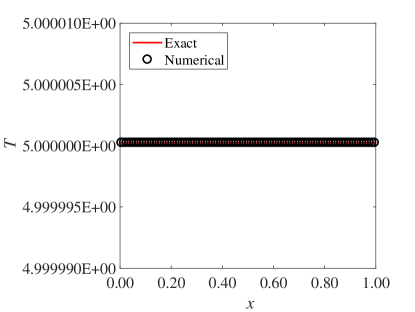
(a) Velocity

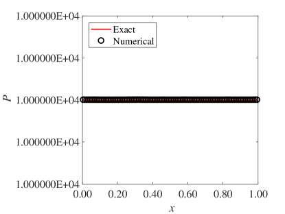
(b) Velocity, locally enlarged

Figure 3: Numerical results for the pure translation of a diffused interface.

4.2 The pure mass diffusion problem

To verify the mass diffusion part of the model, we consider a problem with small diffusion velocity in comparison with the sound speed. In this case, the mass diffusion problem can be approximately treated as an incompressible one. The densities, adiabatic coefficients and specific heat capacities are the same as those in the last test.

It is assumed that mass diffusion goes at very small scale that the pressure and temperature are nearly uniform. In the incompressible limit of such a problem the governing equations are reduced to [43, 42, 3]:

$$\frac{\partial{\rho}}{\partial t}=\frac{\partial}{\partial x}\left(D\frac{\partial{\rho}}{\partial x}\right),\quad\frac{\partial}{\partial x}\left({u}+\frac{D}{{\rho}}\frac{\partial{\rho}}{\partial x}\right)=0.$$ (116)

With the zero-gradient boundary condition for the density, the solution to eq. 116 is given by eq. 115. To investigate the convergence performance of the models, the initial conditions are given with the integration of eq. 115 and averaging within each cell [3]. The initial pressure is uniformly set to be $1\times 10^{5}\text{Pa}$, which results in small enough Mach number so that the compressibility effect can be neglected. Computations are performed on a series of refining grid. The corresponding numerical results are demonstrated in Figure 4. It can be seen that the numerical results tend to converge to the analytical solution (in the incompressible limit) with the grid refinement with the second-order MUSCL for spatial reconstruction in the hydrodynamic stage. The convergence order of the numerical algorithm is approximately 2, as demonstrated in Figure 5a. We also compare the temperature error with the results in [3] (Figure 5b).

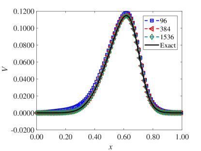
(a) Velocity

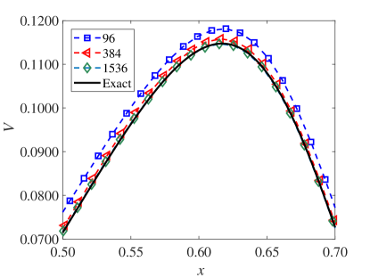
(b) Velocity, locally enlarged

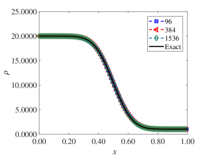
(c) Density

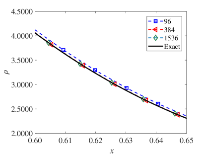
(d) Density, locally enlarged

Figure 4: Numerical results for the pure mass diffusion problem.

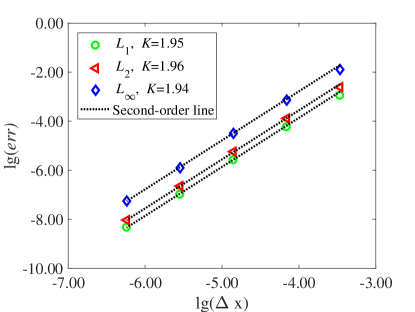
(a) Accuracy order

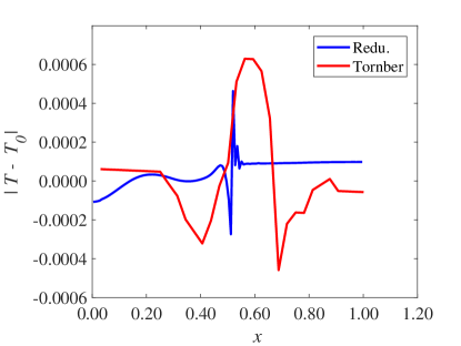
(b) Temperature error

Figure 5: Numerical results of the reduced model for the pure mass diffusion problem. Left: convergence rate. Right: temperature error on 128-cell grid when $P=1\times 10^{4}$.

4.3 The convergence of the viscous part

Having validated the convergence of the mass diffusion, we then check the convergence performance of the viscous part. For such purpose, we manufacture an exact solution as follows

$$\left\{\begin{array}[]{l}(\alpha_{k}\rho_{k})(x,t)=0.5\text{kg}/\text{m}^{3},\\ \alpha_{1}(x,t)=0.7,\\ p(x,t)=100\text{Pa},\\ u(x,t)=\frac{1+(2a-1)\exp((1-a)\xi/v)}{1+\exp((1-a)\xi/v)},\quad\xi=x-at-x_{0}.\end{array}\right.$$ (117)

Note the the manufactured solution for $u(x,t)$ is the analytical solution to the viscous Burgers equation

$$\frac{\partial{u}}{\partial{t}}+\frac{\partial}{\partial x}\frac{u^{2}}{2}=\nu\frac{\partial^{2}u}{\partial x^{2}}.$$

The properties for the materials are given as $\gamma_{1}=5.0$, $C_{v,1}=40.0\text{J}/(\text{kg}\cdot\text{K})$, $\gamma_{1}=1.4$, $C_{v,1}=400.0\text{J}/(\text{kg}\cdot\text{K})$ so that the initial temperature equilibrium is satisfied. We use the constants $a=0.4$, $x_{0}=0.1\text{m}$ and $\nu=0.01\text{}$, the exact solution at $t=0.05\text{s}$ is taken as the initial value. We perform computation to $t=0.15\text{s}$. The numerical results tend to converge to the exact solution with grid refinement (Figure 6b). The dependence of the error on the spatial resolution is demonstrated in Figure 6a, demonstrating the accuracy order is approximately second order.

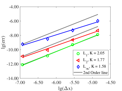
(a) Accuracy order

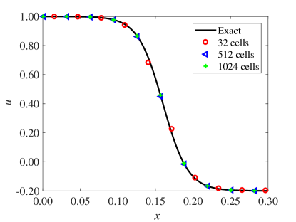
(b) Velocity on different grids

Figure 6: Convergence performance of the viscous part.

4.4 The multi-component shock tube problem

To verify and compare different models, we consider a multicomponent shock tube problem with a resolved interface. The initial condition is given as follows

$$\left(\rho,u,p,\gamma,C_{v}\right)=\begin{cases}\left(1000\mathrm{~{}kg}\cdot\mathrm{m}^{-3},0\mathrm{~{}m}\cdot\mathrm{s}^{-1},10^{9}\mathrm{~{}Pa},4.4,1606\text{J}/(\text{kg}\cdot\text{K})\right)&\text{ for }x<0.7,\\ \left(50\mathrm{~{}kg}\cdot\mathrm{m}^{-3},0,10^{5}\mathrm{~{}Pa},1.4,714\text{J}/(\text{kg}\cdot\text{K})\right)&\text{ for }0.7<x<1.\end{cases}$$ (118)

We have used two sets of grid, i.e., a coarse grid of 1200 uniform cells and a fine one of 12000. The numerical results obtained with different models are demonstrated in Figure 7. The exact solutions in this figure are those of the multi-component Euler equation without any relaxations and (numerical or physical) diffusion. Therefore, the solution of the hydrodynamic part (eq. 67) without any relaxation agrees better with the exact solutions (Figure 7b).

The numerical results of the one-temperature four-equation model and the temperature-disequilibrium model with the complete temperature relaxation deviate from the exact solution in the vicinity of the interface. Moreover, the one-temperature model introduce overshoot in temperature (Figure 7d).

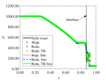
(a) density

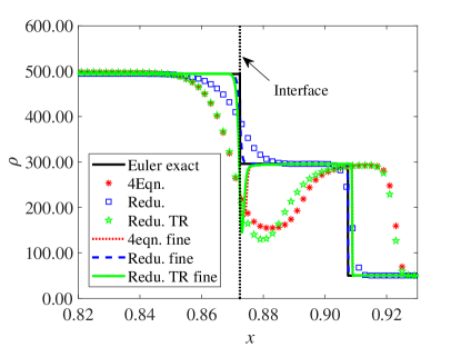
(b) density, locally enlarged

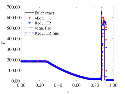
(c) Temperature

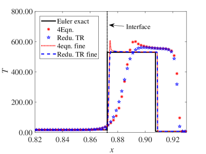
(d) Temperature, locally enlarged

Figure 7: Numerical results obtained with different models on different grids for the shock tube problem.

4.5 Shock passage through a smeared interface

The mass diffusion creates a physically smeared interface. The interaction between such smeared interface and the shock is experimentally investigated in literature, for example, the gas curtain experiment [44]. The current test is a 1D analogue of this problem. The initial condition is demonstrated in Figure 8. A shock in air of Mach 5 impact the smeared SF₆ zone, within which the volume fraction is distributed as [45]

$$\alpha_{\text{SF}_{6}}=\frac{C}{\text{exp}{\left[(836(x-0.02))^{2}\right]}}.$$ (119)

Here we take the constant $C$ to be 0.95.

The incident shock transmits and reflects in its interaction with the smeared interface. It compresses the smeared interface to form a thin spike in density. We compare the solutions obtained with the one-temperature four-equation model and the reduced model without/without the temperature relaxation. The numerical results for density, temperature and mass fraction are compared in Figures 9a and 9b, Figures 9c and 9d and Figures 9e and 9f, respectively. We see that the the solutions of the reduced model without the temperature relaxation deviate from those with the temperature relaxation being included implicitly (for the four-equation model) or explicitly (for the reduced model). From Figure 9d one can observe obvious oscillations in the solutions of the four-equation model.

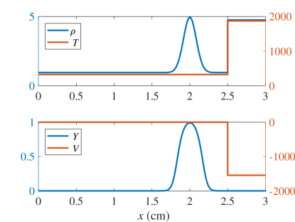
Figure 8: Initial condition for the problem of shock passage through a smeared interface.

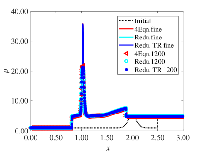
(a) density

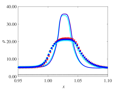
(b) density, locally enlarged

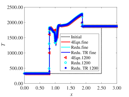
(c) Temperature

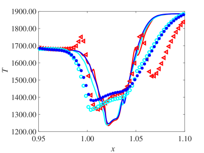
(d) Temperature, locally enlarged

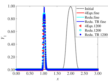
(e) Mass fraction

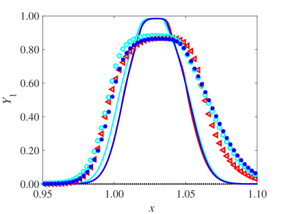
(f) Mass fraction, locally enlarged

Figure 9: Numerical results for the shock passage through a smeared interface.

4.6 The shock wave passage through a helium bubble

In this section, we consider the interaction of a shock (Mach number 1.22) and a cylindrical helium bubble [46, 47]. The computational domain is of size $22.25\mathrm{~{}cm}\times 8.90\mathrm{~{}cm}$. The bubble with the diameter 5cm is initially located at $(13.80\mathrm{~{}cm},4.45\mathrm{~{}cm})$. The initial data is given as:

$$\left(\rho,u,p,\gamma,C_{v}\right)=\begin{cases}\left(1.66\mathrm{~{}kg}\cdot\mathrm{m}^{-3},-114\mathrm{~{}m}\cdot\mathrm{s}^{-1},159080.98\mathrm{~{}Pa},1.4,2430.35\text{J}/(\text{Kg}\cdot\text{K})\right)&\text{ for }x>x_{s}\\ \left(1.2062\mathrm{~{}kg}\cdot\mathrm{m}^{-3},0,101325\mathrm{~{}Pa},1.4,2430.35\text{J}/(\text{Kg}\cdot\text{K})\right)&\text{ in air, for }x\leq x_{s}\\ \left(0.2204\mathrm{~{}kg}\cdot\mathrm{m}^{-3},0,101325\mathrm{~{}Pa},1.6451,717.50\text{J}/(\text{Kg}\cdot\text{K})\right)&\text{ inside the helium bubble }\end{cases}$$ (120)

where the $x_{s}=16.80$cm is the initial position of the left-going shock wave.

We compute this problem including viscosity, heat conduction and mass diffusion. The viscosity coefficient is determined with Sutherland’s equation [48]. The heat conduction coefficient is determined in the same way as in [47]. As for the mass diffusivity, since its dependence on temperature and pressure is $D\sim{T^{3/2}}/{p}$, we calculate it with

$$D=D_{0}\frac{T^{3/2}/p}{T_{0}^{3/2}/p_{0}},$$ (121)

where $D_{0}$ is a reference value at $(p_{0},T_{0})$. We use $D_{0}=73.35\times 10^{-6}$m²/s at $p=1$atm and $T=298$K [49].

To verify the numerical results we compare the numerically obtained interface motion of the bubble along the horizontal centreline with those of [47] (Figure 10). Note that computations of [47] is performed without mass diffusivity. Since the shock-interface interaction time is very short, the impact of mass diffusivity on the interface motion is marginal. However, it does modify the small-scale flow structures (Figure 12). From the 1D slice along the horizontal centreline, one can see that the diffusivity smears the density profile.

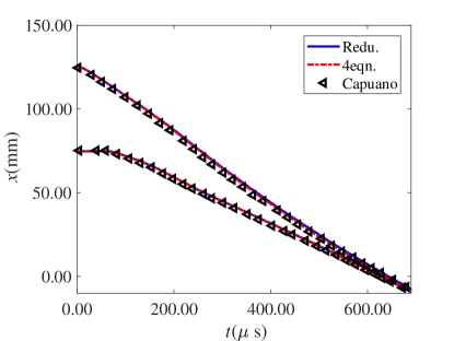
Figure 10: The time evolution of the interface position along the horizontal centreline. The lines on the top(bottom) correspond to the positions of the right(left) interface.

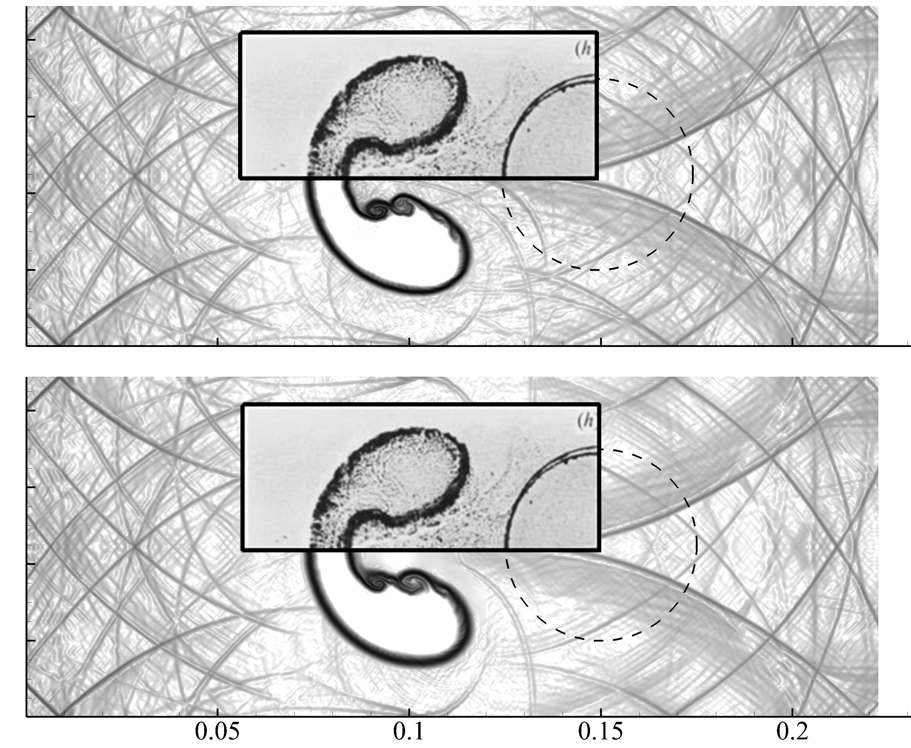
Figure 11: The numerical Schlieren obtained with the four-equation model (top) and the five-equation model (bottom) compared with the experimental shadow graph (inside the rectangular area). The dashed circle is the initial position of the bubble.

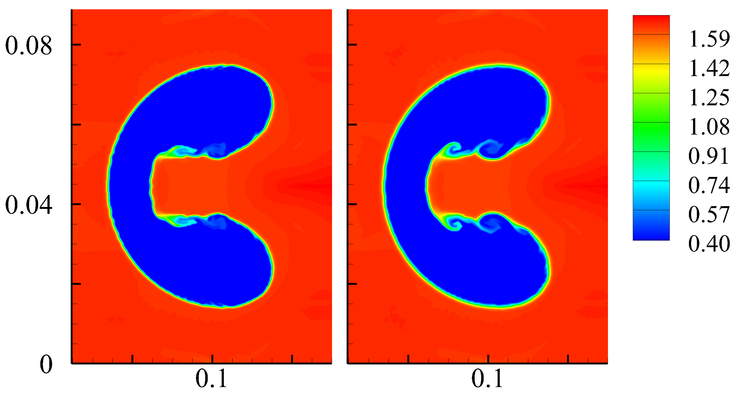
(a) The solutions for density in the cases of diffusivity being excluded (left) and included (right)

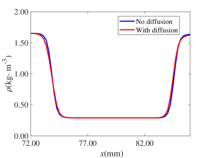
(b) The density distribution along the horizontal centreline

Figure 12: The experiment of RM instability on Omega.

The solutions for the temperature obtained with different models in the neighbourhood of the bubble are compared in Figure 13. Serious non-physical oscillations arise in across the interface in the solutions of the four-equation model, which is more clear in the 1D distribution along the horizontal centreline in Figure 13b. When temperature diffusivity is significant enough, this non-physical error may have a major impact on the convergence of the model.

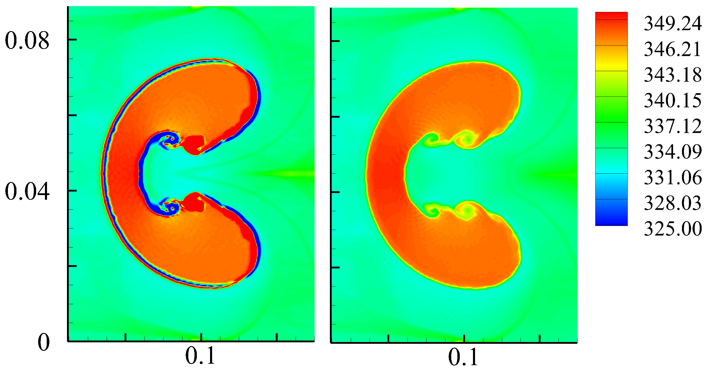
(a) Temperature distribution (at the time moment $t=427\mu$s timing from the beginning of the shock-interface interaction) obtained with the four-equation model (left) and the reduced five-equation model (right).

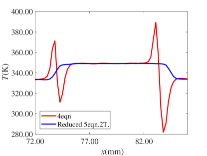
(b) The temperature distribution along the centreline of the bubble

Figure 13: Numerical results for temperature.

4.7 The laser-driven RM instability problem

In this section we consider the laser-driven RM instability problem conducted on OMEGA [50, 51]. The schematic for the experiment is demonstrated in Figure 14. The multi-material target is assembled into a Beryllium shock tube of diameter 800$\mu$m. The target is made up of two sections: the pusher section of length 150$\mu$m on the right and the payload section of length 19mm on the left. A strong shock is generated by laser ablation of the pusher section that consists of the polyimide (C₂₂H₁₀N₂O₄) and the polystyrene (C₅₀₀H₄₅₇Br₄₃). This section is modeled as a homogeneous material with density 1.41$\text{g}/\text{cm}^{3}$ and $\gamma=5/3$. The remainder of the target is carbon foam payload (C-foam, $\rho=0.1\text{g}/\text{cm}^{3},\;\gamma=1.4$) . The interface between two sections is initially perturbed as a cosine function with wavelength 50$\mu$m and amplitude 2$\mu$m. The laser has a wavelength of 0.351$\mu$m and average intensity $6\times 10^{14}$W/cm². The shock in the central area has good planarity, and thus is approximated as a planar one.

Note that there are many complicated experimental uncertainties that are difficult to account for in numerical simulations, for example, the pre-heating state of the target and the laser energy loss. Moreover, with the polytropic equation of state, the true state of the materials are described with limited accuracy. Moreover, the experiment diagnosis also introducesss some error. Due to these uncertainties, numerical simulations can hardly reproduce the experimental conditions. We set the initial temperature to be 290K based on a trial-and-error approach.

Our simulation focuses on one period of the perturbation with periodical boundary conditions being imposed on sides perpendicular to the incident shock. The present simulation includes a complete physical processes: laser energy deposition, heat conduction, viscosity and mass diffusion. The laser energy deposits in a 20$\mu$m area to the right of the critical density $\rho_{crt}$ of the ablator. According to the inverse bremsstrahlung absorption theory the critical density is $\rho_{crt}=2.78\times 10^{-2}$g/cm³. The heat conduction coefficient of the plasma is calculated with the Spitzer-Harm model [52]. The plasma viscosity is modeled with Clerouin’s model [53]. As for the mass diffusivity, we use the estimates in [1], prior to the interaction of shock and the interface, the materials are in solid states and the mass diffusivity is negligible. After the shock arrival (at $t\approx 2$ns), the Schmidt number ($Sc=\nu/D$, $\nu$ is the average kinetic viscosity) is almost constant 1. In this estimation, the mass diffusivity is determined with the model of Paquette [54].

Computations are performed on a grid of $2880\times 60$ cells with the proposed reduced model and the conservative four-equation model. The numerical results for density, temperature and mass fraction are displayed in Figure 15. It can be seen that the solutions of both models have similar flow structures. The shock wave and the interface move slightly faster in the solutions of the reduced model than that in the solutions of the four-equation model.

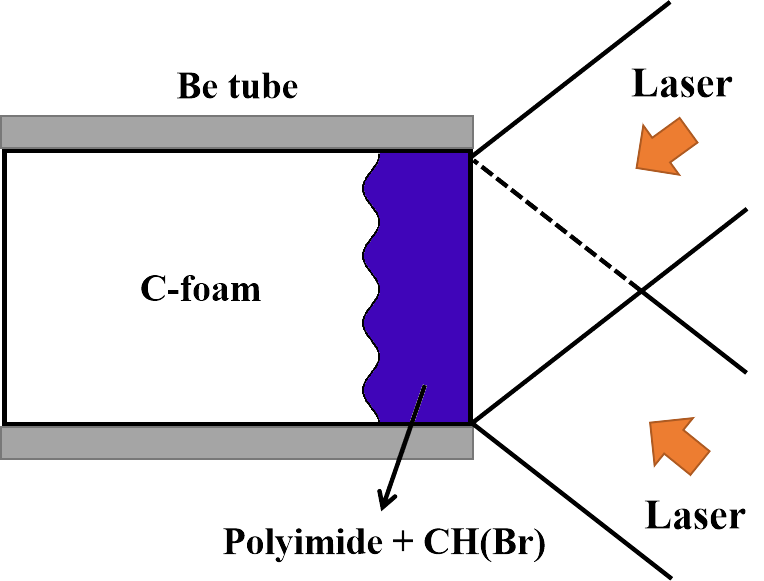
Figure 14: The schematic of the laser-driven RM instability experiment on Omega.

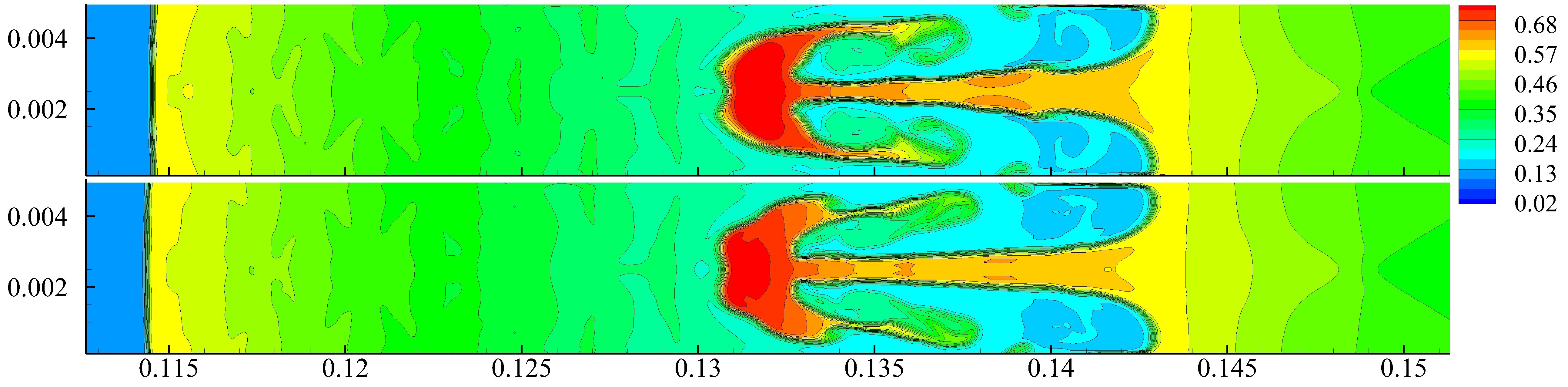
(a) Density

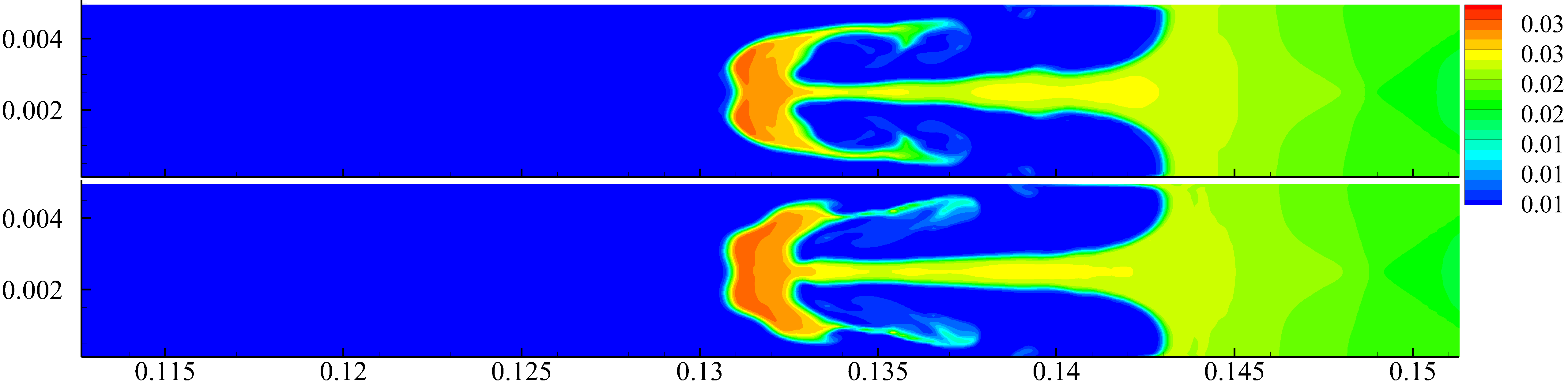
(b) Temperature

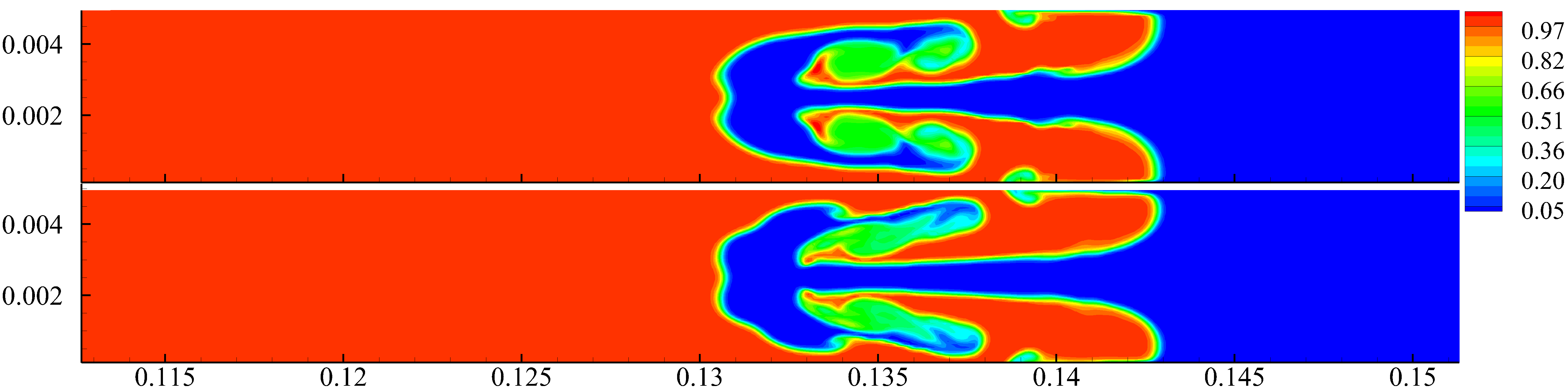
(c) Mass fraction

Figure 15: Numerical results for the density, the temperature and the mass fraction when $t=12$ns for the laser-driven RM instability problem. Top figures are results of the four-equation model, bottom ones are that of the reduced model. The dimension for length, density and temperature are cm, g/cm³ and MK, respectively.

In Figure 16 we compare the numerically obtained interface evolution parameters with the experimental ones. Figure 16a demonstrates the evolution of the leftmost interface position (i.e., the distance from its initial position) with time. Good agreement with the experimental results are observed. Figure 16b shows the time evolution of the half peak-to-valley amplitude. Both models give results that lie within the measurement range.

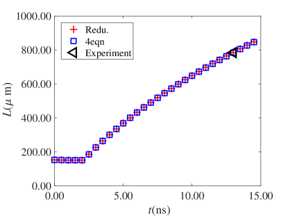
(a) Interface position

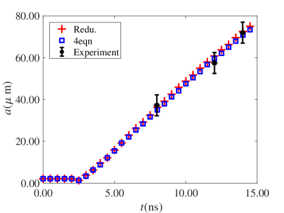
(b) Amplitude

Figure 16: The time evolution of the interface position and amplitude of the laser-driven RM instability problem.

We define the Reynolds number $Re=uL/\nu$, where $u$ is the characteristic velocity $\frac{1}{2}\rho u^{2}=E$, $E$ is the the total deposited laser energy, $\rho$ is the average mixture density, the characteristic length $L$ is taken to be the wavelength of the initial perturbation and the $\nu$ the initial maximum mixture kinetic viscosity. To investigate the impact of the diffusivity, we increase $Re$ through the viscosity. The numerical solutions for the mass fraction in the case of different diffusivities are compared in Figure 17. We can see that the transport process tend to wipe out the small flow structures. The last two figures compare the numerical results with and without the mass diffusion, whose effect in smearing the mass fraction is evident.

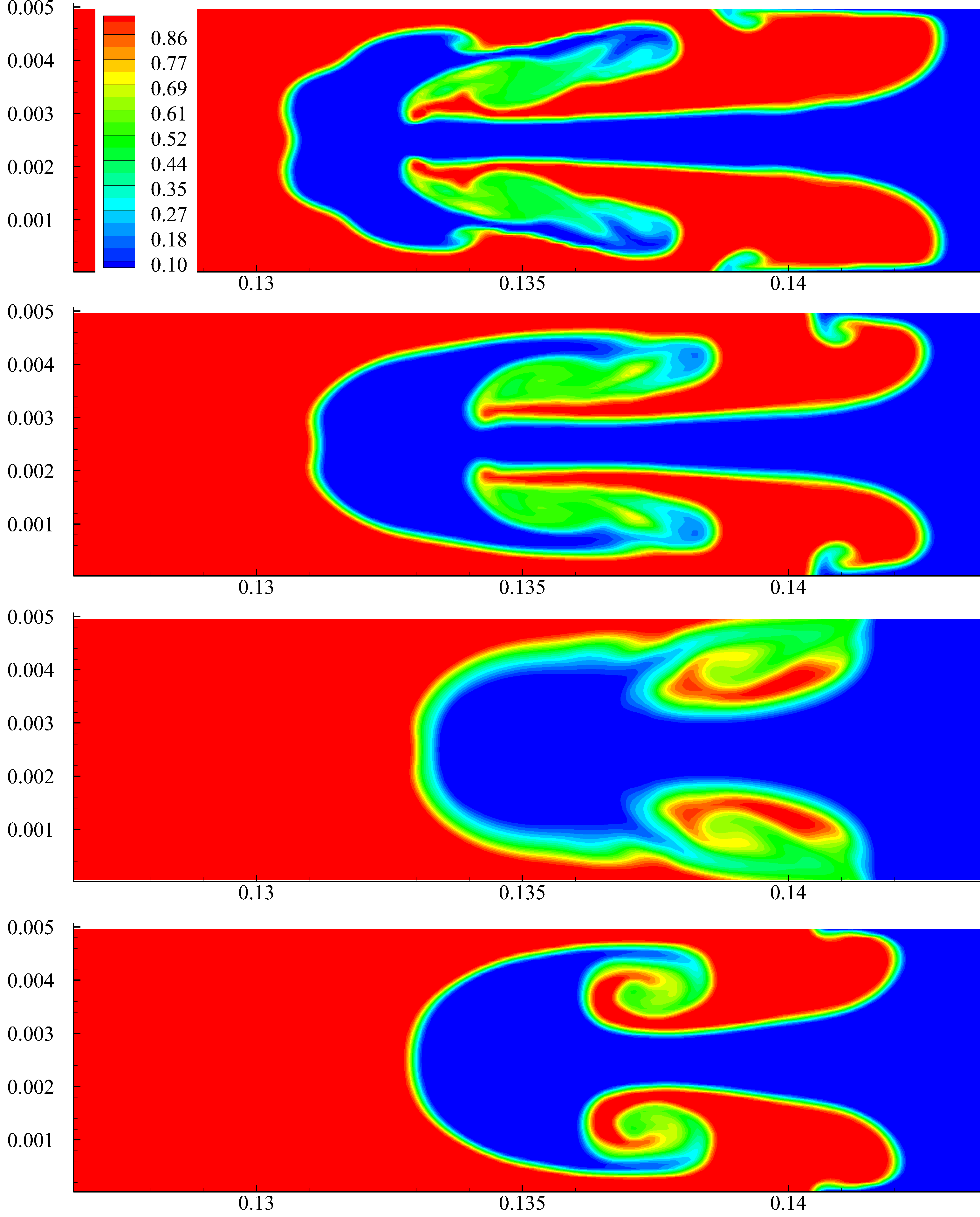
Figure 17: numerical solutions for the mass fraction of the C-foam in the case of different diffusivities. The Reynolds number for the experiment condition is used as the reference $Re_{exp}$. From top to bottom: (1) $Re=Re_{exp},\;Sc=1$, (2) $Re=Re_{exp}/10,\;Sc=1$, (3) $Re=Re_{exp}/50,\;Sc=1$, (4) $Re=Re_{exp},\;1/Sc\to 0$.

5 Conclusion

In the present paper we have presented a diffuse-interface model for compressible multicomponent flows with interphase heat transfer, external energy source, and diffusions (including viscous, heat conduction, mass diffusion, enthalpy diffusion processes). The model is reduced from the Baer-Nunziato model in the limit of instantaneous mechanical relaxations. Difference between time scales of velocity, pressure and temperature relaxations has been accounted for. The reduction procedure results in a temperature-disequilibrium, velocity-disequilibrium, and pressure-equilibrium five-equation model. The proposed model if free of the spurious oscillation problem in the vicinity of the interface and respects the laws of thermodynamics. Numerical methods for its solution have been proposed on the basis of the fractional step method. The model is split into five parts including the hydrodynamic part, the viscous part, the temperature relaxation part, the heat conduction part and the mass diffusion part. The hyperbolic equations involved are solved with the Godunov finite volume method, and the parabolic ones with the locally iterative method based on Chebyshev parameters. The developed model and numerical methods have been used for solving several multicomponent problems and verified against analytical and experimental results. Moreover, we have applied our model to simulate the laser ablation process of a multicomponent target, where the Richtmyer-Meshkov instability can be evidently observed. Comparison with experimental results demonstrates that our model captures physical phenomenon of this process.

References

• [1] HF Robey. Effects of viscosity and mass diffusion in hydrodynamically unstable plasma flows. Physics of plasmas, 11(8):4123–4133, 2004.
• [2] E Vold, L Yin, and BJ Albright. Plasma transport simulations of rayleigh–taylor instability in near-icf deceleration regimes. Physics of Plasmas, 28(9):092709, 2021.
• [3] Ben Thornber, Michael Groom, and David Youngs. A five-equation model for the simulation of miscible and viscous compressible fluids. Journal of Computational Physics, 372, 03 2018.
• [4] Andrew Cook. Enthalpy diffusion in multicomponent flows. Physics of Fluids, 21, 12 2008.
• [5] R. Abgrall. How to prevent pressure oscillations in multicomponent flow calculations: a quasi conservative approach. Journal of Computational Physics, 125(1):150–160, 1996.
• [6] Rémi Abgrall and Smadar Karni. Computations of compressible multifluids. Journal of computational physics, 169(2):594–623, 2001.
• [7] R. Saurel and R. Abgrall. A multiphase godunov method for compressible multifluid and multiphase flows. Journal of Computational Physics, 150(2):425–467, 1999.
• [8] AK Kapila, R Menikoff, JB Bdzil, SF Son, and D Scott Stewart. Two-phase modeling of deflagration-to-detonation transition in granular materials: Reduced equations. Physics of fluids, 13(10):3002–3024, 2001.
• [9] M.R. Baer and J.W. Nunziato. A two-phase mixture theory for the deflagration-to-detonation transition (DDT) in reactive granular materials. International Journal of Multiphase Flow, 12(6):861 – 889, 1986.
• [10] R. Saurel, F. Petitpas, and R. Berry. Simple and efficient relaxation methods for interfaces separating compressible fluids, cavitating flows and shocks in multiphase mixtures. Journal of Computational Physics, 228(5):1678–1712, 2009.
• [11] A. Murrone and H. Guillard. A five equation reduced model for compressible two phase flow problems. Journal of Computational Physics, 202(2):664–698, 2005.
• [12] G. Perigaud and R. Saurel. A compressible flow model with capillary effects. Journal of Computational Physics, 209(1):139–178, 2005.
• [13] Zbigniew Bilicki, Roman Kwidziński, and Salim Ali Mohammadein. Evaluation of the relaxation time of heat and mass exchange in the liquid-vapour bubble flow. International journal of heat and mass transfer, 39(4):753–759, 1996.
• [14] Hervé Guillard and Mathieu Labois. Numerical modelling of compressible two-phase flows. 2006.
• [15] Ali Zein, Maren Hantke, and Gerald Warnecke. Modeling phase transition for compressible two-phase flows applied to metastable liquids. Journal of Computational Physics, 229(8):2964–2998, 2010.
• [16] V. Coralic and T. Colonius. Finite-volume weno scheme for viscous compressible multicomponent flows. Journal of Computational Physics, 274:95–121, 2014.
• [17] J. J Kreeft and B. Koren. A new formulation of kapila’s five-equation model for compressible two-fluid flow, and its numerical treatment. Journal of Computational Physics, 229(18):6220–6242, 2010.
• [18] C. Zhang and I. Menshov. Eulerian model for simulating multi-fluid flows with an arbitrary number of immiscible compressible components. Journal of Scientific Computing, 83(2):1–33, 2020.
• [19] V. T. Zhukov. Explicit methods for the numerical integration of parabolic equations. Mat. Model., 22:127–158, 2010.
• [20] V. T. Zhukov, O. B. Feodoritova, A. P. Duben, and N. D. Novikova. Explicit time integration of the Navier-Stokes equations using the local iteration method. KIAM Preprint, 12:1–32, 12 2019.
• [21] Fabien Petitpas and Sebastien Le Martelot. A discrete method to treat heat conduction in compressible two-phase flows. Computational Thermal Sciences, 6:251–271, 2014.
• [22] Donald A Drew. Mathematical modeling of two-phase flow. Annual review of fluid mechanics, 15(1):261–291, 1983.
• [23] R. Saurel and C. Pantano. Diffuse-interface capturing methods for compressible two-phase flows. Annual Review of Fluid Mechanics, 50:105–130, 2018.
• [24] Richard Saurel, Sergey Gavrilyuk, and François Renaud. A multiphase model with internal degrees of freedom: application to shock–bubble interaction. Journal of Fluid Mechanics, 495:283–321, 2003.
• [25] C. Zhang. Mathematical modeling of heterogeneous multi-material flows (in Russian). PhD thesis, Lomonosov Moscow State University, 2019.
• [26] F.A. Williams. Combustion theory. The Benjamin/Cummings Publishing Company, inc, 1985.
• [27] F Petitpas, Richard Saurel, Erwin Franquet, and A Chinnayya. Modelling detonation waves in condensed energetic materials: Multiphase cj conditions and multidimensional computations. Shock waves, 19(5):377–401, 2009.
• [28] J.A. Geurst. Variational principles and two-fluid hydrodynamics of bubbly liquid/gas mixtures. Physica A: Statistical Mechanics and its Applications, 135(2):455–486, 1986.
• [29] Henri Gouin and Sergey Gavrilyuk. Dissipative two-fluid models, 2008.
• [30] Rémi Abgrall and Smadar Karni. Computations of compressible multifluids. Journal of Computational Physics, 169(2):594–623, 2001.
• [31] E.F. Toro. Riemann Solvers and Numerical Methods for Fluid Dynamics. Springer, 2009.
• [32] E. Johnsen and T. Colonius. Implementation of weno schemes in compressible multicomponent flow problems. Journal of Computational Physics, 219(2):715–732, 2006.
• [33] G.S. Jiang and C.W. Shu. Efficient implementation of weighted eno schemes. Journal of Computational Physics, 126(1):202–228, 1996.
• [34] Randall J LeVeque et al. Finite volume methods for hyperbolic problems, volume 31. Cambridge university press, 2002.
• [35] Arpit Tiwari, Jonathan B. Freund, and Carlos Pantano. A diffuse interface model with immiscibility preservation. Journal of Computational Physics, 252(C):290–309, 2013.
• [36] S. Lemartelot, R. Saurel, and B. Nkonga. Towards the direct numerical simulation of nucleate boiling flows. International Journal of Multiphase Flow, 66(7):62–78, 2014.
• [37] Victor Timofeevich Zhukov and Olga Borisovna Feodoritova. On development of parallel algorithms for the solution of parabolic and elliptic equations. Itogi Nauki i Tekhniki. Seriya” Sovremennaya Matematika i ee Prilozheniya. Tematicheskie Obzory”, 155:20–37, 2018.
• [38] S. Alahyari Beig and E. Johnsen. Maintaining interface equilibrium conditions in compressible multiphase flows using interface capturing. Journal of Computational Physics, 302:548–566, 2015.
• [39] E. Johnsen and F. Ham. Preventing numerical errors generated by interface-capturing schemes in compressible multi-material flows. Journal of Computational Physics, 231(17):5705–5717, 2012.
• [40] G. Allaire, S. Clerc, and S. Kokh. A five-equation model for the simulation of interfaces between compressible fluids. Journal of Computational Physics, 181(2):577–616, 2002.
• [41] Bernard Larrouturou. How to preserve the mass fractions positivity when computing compressible multi-component flows. Journal of computational physics, 95(1):59–84, 1991.
• [42] Ioannis Kokkinakis, Dimitris Drikakis, David Youngs, and R.J.R. Williams. Two-equation and multi-fluid turbulence models for rayleigh–taylor mixing. International Journal of Heat and Fluid Flow, 56:233–250, 12 2015.
• [43] D. Livescu. A multiphase model with internal degrees of freedom: application to shock–bubble interaction. Philosophical transactions. Series A, Mathematical, physical, and engineering sciences, 371:283–321, 2013.
• [44] BJ Balakumar, GC Orlicz, CD Tomkins, and KP Prestridge. Simultaneous particle-image velocimetry–planar laser-induced fluorescence measurements of richtmyer–meshkov instability growth in a gas curtain with and without reshock. Physics of Fluids, 20(12):124103, 2008.
• [45] Karnig O Mikaelian. Numerical simulations of richtmyer–meshkov instabilities in finite-thickness fluid layers. Physics of Fluids, 8(5):1269–1292, 1996.
• [46] J.F. Haas and B. Sturtevant. Interaction of weak shock waves with cylindrical and spherical gas inhomogeneities. Journal of Fluid Mechanics, 181:41 – 76, 09 1987.
• [47] M. Capuano, C. Bogey, and P. D. M. Spelt. Simulations of viscous and compressible gas-gas flows using high-order finite difference schemes. Journal of Computational Physics, 361:56–81, 2018.
• [48] W. Sutherland. The Viscosity of Gases and Molecular Force, volume 36. 1893.
• [49] SP Wasik and KE McCulloh. Measurements of gaseous diffusion coefficients by a gas chromatographic technique. Journal of research of the National Bureau of Standards. Section A, Physics and chemistry, 73(2):207, 1969.
• [50] H. F. Robey, Y. Zhou, A. C. Buckingham, P. Keiter, B. A. Remington, and R. P. Drake. The time scale for the transition to turbulence in a high reynolds number, accelerated flow. Physics of Plasmas, 10(3):614–622, 2003.
• [51] AR Miles, DG Braun, MJ Edwards, HF Robey, RP Drake, and DR Leibrandt. Numerical simulation of supernova-relevant laser-driven hydro experiments on omega. Physics of plasmas, 11(7):3631–3645, 2004.
• [52] L. Spitzer and R. Harm. Transport phenomena in a completely ionized gas. Physical Review, 89(5):977–981, 1953.
• [53] JG Clérouin, MH Cherfi, and G Zérah. The viscosity of dense plasmas mixtures. EPL (Europhysics Letters), 42(1):37, 1998.
• [54] C Paquette, C Pelletier, G Fontaine, and G Michaud. Diffusion coefficients for stellar plasmas. The Astrophysical Journal Supplement Series, 61:177–195, 1986.