The Transitive Information Theory and its Application to Deep Generative Models

Trung Ngo
School of Computing
University of Eastern Finland
Joensuu, Finland
trung@uef.fi
&Najwa Laabid
School of Medicine
University of Eastern Finland
Kuopio, Finland
najwa.laabid@uef.fi
&Ville Hautamäki
School of Computing
University of Eastern Finland
Joensuu, Finland
villeh@cs.uef.fi
&Merja Heinäniemi
School of Medicine
University of Eastern Finland
Kuopio, Finland
merja.heinaniemi@uef.fi
Abstract

Paradoxically, a Variational Autoencoder (VAE) could be pushed in two opposite directions, utilizing powerful decoder model for generating realistic images but collapsing the learned representation, or increasing regularization coefficient for disentangling representation but ultimately generating blurry examples. Existing methods narrow the issues to the rate-distortion trade-off between compression and reconstruction. We argue that a good reconstruction model does learn high capacity latents that encode more details, however, its use is hindered by two major issues: the prior is random noise which is completely detached from the posterior and allow no controllability in the generation; mean-field variational inference doesn’t enforce hierarchy structure which makes the task of recombining those units into plausible novel output infeasible. As a result, we develop a system that learns a hierarchy of disentangled representation together with a mechanism for recombining the learned representation for generalization. This is achieved by introducing a minimal amount of inductive bias to learn controllable prior for the VAE. The idea is supported by here developed transitive information theory, that is, the mutual information between two target variables could alternately be maximized through the mutual information to the third variable, thus bypassing the rate-distortion bottleneck in VAE design. In particular, we show that our model, named SemafoVAE (inspired by the similar concept in computer science), could generate high-quality examples in a controllable manner, perform smooth traversals of the disentangled factors and intervention at a different level of representation hierarchy.

1 Introduction

Earlier effort in generative model was solely relied on statistical model defined by human experts, inference for such model is tractable by narrow a set of strict assumption regarding the data generation process Bishop (2006). Conversely, modern methods leverage recent advance in computing to approximate the generation process using powerful nonlinear model and big data. The two prominent families of these methods are: implicit generative model such as generative adversarial network (GAN) Goodfellow et al. (2014) and explicit generative model which includes the variational autoencoder (VAE) Kingma and Welling (2014). While the first approach have demonstrated its merits in generating realistic high-quality image Karras et al. (2018), the second one is often referred as a representation learning algorithm that capturing independent factor of variations (FOVs) also known as disentanglement representation Higgins et al. (2017); Locatello et al. (2019).

The benefit of learning independent generative factors are discussed in Bengio et al. (2014) and Schölkopf et al. (2021), these include: boosting the performance of downstream task, improving the robustness of generative model under distribution shift and discovering the causal variables. Thus, we could reasonably assume that a model that learn relevant factors for generating data would have better understanding of the data manifold by itself, subsequently, enabling it to generate better images. However, this isn’t the case for the known families of generative methods. First, GAN doesn’t explicitly learn a meaningful representation, the whole generation process is distilled into the deep generator network which have been known to suffer from mode collapse issue Goodfellow (2017). In contrast, VAE has established to be a reliable performer under various disentanglement representation benchmarks Locatello et al. (2019); Qiao et al. (2019), and its ability to learn a tractable latent distribution enables the representation to be generalized beyond the reconstruction task. This capability doesn’t come without a drawback, pushing the compression rate in VAE is equivalent to forcing the high-distorted outputs Alemi et al. (2017), as a result, the generated image is blurry and lacks detail Burgess et al. (2018).

In practice, VAE is capable of generating high-fidelity images by carefully redesign its architecture Maaløe et al. (2019); Vahdat and Kautz (2020); Child (2021). These designs significantly increase the depth both VAE’s encoder and decoder, and allows the accommodation of the hierarchical latent variables. It is unclear how the complication of design would affect the ability to learn independent meaningful factors of VAE, and these models haven’t been evaluated against the state-of-the-art (SoTA) disentangling methods Locatello et al. (2019). Preliminary studies in Havtorn et al. (2021) indicates that hierarchical VAE does learn hierarchical representation by adding layers of fine details to the mode of learned distribution, however, this raises more important question about how to navigate through a large number of possible latent units combinations to sample the attributes of interest. To revisit the initial claim, we reason that generative model doesn’t need to generate all the possible images but only the images with particular attributes in a controllable manner for real life setting. Additionally, our lack of understanding of such high-resolution representation is apparently the missing of a learnable controlling mechanism for generation Montero et al. (2021), i.e. a compositional mechanism that recombining disentangled and hierarchical representation in a meaningful way.

The method presented in this paper addressing three major issues with the conventional VAE framework: 1) learning the hierarchy of factors that are disentangled; 2) learning the compositional mechanism to control the learned representation and 3) all these developments are achieved while improving the expressiveness of VAE generator. In summary, our contributions are following:

  1. 1.

    We provide theoretical and empirical justification for the limitation of VAE framework (Section 2).

  2. 2.

    We develop the transitive information theory explaining how information is transferred among variables. Based on the proposed principles, we implement semi-supervised “SemafoVAE” that encapsulate variables’ hierarchy in its prior and allow explicit control of the generation. (Section 3).

  3. 3.

    The algorithm is benchmarked against the SoTAs in terms of test log-likelihood, generation quality and disentanglement metrics (Section 5).

2 Background: VAE and its limitations

In this section, we review prior work and discuss the VAE’s limitations as a method for generative modeling and representation learning.

2.1 Variational autoencoder

Variational autoencoder Kingma and Welling (2014) introduces the latent variables 𝐳𝐳\mathbf{z} that enables learning richer representation of the observation 𝐱𝐱\mathbf{x}. In the latent variable framework, we obtain marginal pθ(𝐱)=𝐳pθ(𝐱|𝐳)p(𝐳)𝑑𝐳subscript𝑝𝜃𝐱subscript𝐳subscript𝑝𝜃conditional𝐱𝐳𝑝𝐳differential-d𝐳p_{\theta}(\mathbf{x})=\int_{\mathbf{z}}p_{\theta}(\mathbf{x}|\mathbf{z})p(\mathbf{z})d\mathbf{z}, however, the marginalization of the likelihood is intractable. Variational method approximates the posterior distribution pθ(𝐳|𝐱)subscript𝑝𝜃conditional𝐳𝐱p_{\theta}(\mathbf{z}|\mathbf{x}) with a tractable distribution qϕ(𝐳)subscript𝑞italic-ϕ𝐳q_{\phi}(\mathbf{z}), and treats the issue of closing the approximation gap as an optimization problem w.r.t the parameters ϕitalic-ϕ\phi. However, the latent variables are optimized per-data point which is another obstacle for scaling the algorithm. Instead, amortized inference learns the mapping qϕ(𝐳|𝐱)subscript𝑞italic-ϕconditional𝐳𝐱q_{\phi}(\mathbf{z}|\mathbf{x}), and added to the scalability is stochastic optimization for minimizing the posterior divergence D𝙺𝙻(qϕ(𝐳|𝐱)||pθ(𝐳|𝐱))\mathrm{D}_{\mathtt{KL}}({q_{\phi}(\mathbf{z}|\mathbf{x})}||{p_{\theta}(\mathbf{z}|\mathbf{x})}). The log-likelihood of our data is decomposed into two terms as in Kingma and Welling (2014),

logpθ(𝐱)Eqϕ(𝐳|𝐱)[logpθ(𝐱|𝐳)]reconstructionD𝙺𝙻(qϕ(𝐳|𝐱)||p(𝐳))regularisation=(𝐱,𝐳;ϕ,θ),\displaystyle\log p_{\theta}(\mathbf{x})\geq\underbrace{\overbrace{\mathrm{E}_{q_{\phi}(\mathbf{z}|\mathbf{x})}\big{[}\mathrm{log}p_{\theta}(\mathbf{x}|\mathbf{z})\big{]}}^{reconstruction}-\overbrace{\mathrm{D}_{\mathtt{KL}}({q_{\phi}(\mathbf{z}|\mathbf{x})}||{p(\mathbf{z})})}^{regularisation}}_{=\mathcal{E}(\mathbf{x},\mathbf{z};\phi,\theta)}, (1)

where (𝐱,𝐳;ϕ,θ)𝐱𝐳italic-ϕ𝜃\mathcal{E}(\mathbf{x},\mathbf{z};\phi,\theta) defines the evidence lower bound (ELBO), which is maximized for each data point w.r.t the parameters using Monte Carlo estimate and stochastic gradient descent (SGD). The VAE Kingma and Welling (2014) uses reparameterization trick to jointly optimize qϕ(𝐳|𝐱)subscript𝑞italic-ϕconditional𝐳𝐱q_{\phi}(\mathbf{z}|\mathbf{x}) and pθ(𝐱|𝐳)subscript𝑝𝜃conditional𝐱𝐳p_{\theta}(\mathbf{x}|\mathbf{z}), where ϕitalic-ϕ\phi and θ𝜃\theta are parameters of two deep neural networks, and the combination of these techniques enables variational inference (VI) to be both flexible and scalable.

Throughout this study, we denote 𝐱𝐱\mathbf{x} as random variables (RVs) represent the observations which are i.i.d samples from the dataset 𝒟𝒟\mathcal{D} with empirical data distribution q𝒟(𝐱)=1NiNδ(xi)subscript𝑞𝒟𝐱1𝑁superscriptsubscript𝑖𝑁𝛿subscript𝑥𝑖q_{\mathcal{D}}(\mathbf{x})=\frac{1}{N}\sum_{i}^{N}\delta(x_{i}). Then, 𝐳𝐳\mathbf{z} as the latent RVs, and 𝐲𝐲\mathbf{y} are the ground truth factors often understood as the true low-dimensional manifold embedding of 𝐱𝐱\mathbf{x} Dai and Wipf (2019). For the clarity of notation, our derivations in the next sections will omit the parameters ϕitalic-ϕ\phi and θ𝜃\theta.

2.2 Rethinking the ELBO objective

Refer to caption
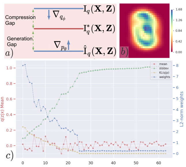
Figure 1: a)a) illustration of the competing objectives between the encoder qϕsubscript𝑞italic-ϕq_{\phi} and decoder pθsubscript𝑝𝜃p_{\theta} of the VAE, where \nabla indicates the corresponding gradient direction, and Iq(𝐱;𝐳)subscriptsuperscriptI𝑞𝐱𝐳\mathrm{I}^{*}_{q}(\mathbf{x};\mathbf{z}) is the optimal balance between compression and generation quality. b)b) heatmap of reconstruction negative log-likelihood on MNIST test set, red color indicate smaller values. c)c) shows the latent units’ statistics of VAE trained on MNIST, weights are the L2-norm of decoder weights placed for each individual latent units (there are 64 units in total, and 25 units are activated).
Lemma 1.

For any encoder model q(𝐳|𝐱)𝑞conditional𝐳𝐱q(\mathbf{z}|\mathbf{x}) and decoder model p(𝐱|𝐳)𝑝conditional𝐱𝐳p(\mathbf{x}|\mathbf{z}), optimizing ELBO is equal to the minimization of

(𝒟,ϕ,θ)𝒟italic-ϕ𝜃\displaystyle\mathcal{L}(\mathcal{D},\phi,\theta) =Eq(𝐱,𝐳)[logq(𝐱,𝐳)q(𝐱)q(𝐳)]=Iq(𝐱,𝐳)(a)Eq(𝐱,𝐳)[logp(𝐱,𝐳)q(𝐳)q(𝐱)]=I^q(𝐱,𝐳)(b)Eq(𝐱)[logq(𝐱)]fixedabsentsubscriptsubscriptE𝑞𝐱𝐳delimited-[]log𝑞𝐱𝐳𝑞𝐱𝑞𝐳absentsubscriptIq𝐱𝐳asubscriptsubscriptE𝑞𝐱𝐳delimited-[]log𝑝𝐱𝐳𝑞𝐳𝑞𝐱absentsubscript^I𝑞𝐱𝐳bsubscriptsubscriptE𝑞𝐱delimited-[]log𝑞𝐱fixed\displaystyle=\underbrace{\mathrm{E}_{q(\mathbf{x},\mathbf{z})}\bigg{[}\mathrm{log}\frac{q(\mathbf{x},\mathbf{z})}{q(\mathbf{x})q(\mathbf{z})}\bigg{]}}_{=\mathrm{I}_{\mathrm{q}}(\mathbf{x},\mathbf{z})\;\mathrm{(a)}}-\underbrace{\mathrm{E}_{q(\mathbf{x},\mathbf{z})}\bigg{[}\mathrm{log}\frac{p(\mathbf{x},\mathbf{z})}{q(\mathbf{z})q(\mathbf{x})}\bigg{]}}_{=\hat{\mathrm{I}}_{q}(\mathbf{x},\mathbf{z})\;\mathrm{(b)}}-\underbrace{\mathrm{E}_{q(\mathbf{x})}\bigg{[}\mathrm{log}q(\mathbf{x})\bigg{]}}_{\text{fixed}} (2)

which jointly: i) pushes the encoder to compress the latent codes by disregarding observational information; and ii) recovers missing information in the latent codes using the generator. (Proof is in the Appendix A.1)

First, lemma 1 indicates maximizing ELBO is the equivalent of minimizing the posterior mutual information Iq(𝐱,𝐳)subscriptIq𝐱𝐳\mathrm{I}_{\mathrm{q}}(\mathbf{x},\mathbf{z}) (term a)a) in (2). This fact was first mentioned in Hoffman and Johnson (2016), and it is indeed the desire property of ELBO that facilitate generalization as interpreted by Alemi et al. (2017, 2019). According to the information bottleneck principle Tishby et al. (1999), the ELBO is max(I(𝐱,𝐳)βI(𝐳,𝐢))maxI𝐱𝐳𝛽I𝐳𝐢\mathrm{max}(\mathrm{I}(\mathbf{x},\mathbf{z})-\beta\mathrm{I}(\mathbf{z},\mathbf{i})) where 𝐢𝐢\mathbf{i} is the index to the individual example. However, this interpretation leaves much to be answered since the VAE could solely focus on learning the mean of 𝐱𝐱\mathbf{x} if required to ignore all the individual details. Paradoxically, study in Bozkurt et al. concluded that the best generalized VAE was achieved by severely weakening the KL-regularization term in (1), while other studies in Higgins et al. (2017); Burgess et al. (2018); Higgins et al. (2018); Montero et al. (2021) proposes an opposite approach that increasing regularization of the latents would encourage VAE to learn more generalized representation.

We prove that term b)b) in (2) is actually the lower bound of a)a), i.e. I^q(𝐱,𝐳)Iq(𝐱,𝐳)subscript^I𝑞𝐱𝐳subscriptIq𝐱𝐳\hat{\mathrm{I}}_{q}(\mathbf{x},\mathbf{z})\leq\mathrm{I}_{\mathrm{q}}(\mathbf{x},\mathbf{z}). Since the last quantity is constant for a given dataset, the ELBO game focuses on the interaction between a)a) - the encoder and b)b) - the decoder. Figure 1-a illustrates both players have opposed objective to realize their maximum capacity at the optimal point I(𝐱,𝐳)superscriptI𝐱𝐳\mathrm{I^{*}}(\mathbf{x},\mathbf{z}). The description resembles an adversarial game, in practice, encoder and decoder coordinate together reaching an equilibrium point. If Iq(𝐱,𝐳)subscriptIq𝐱𝐳\mathrm{I}_{\mathrm{q}}(\mathbf{x},\mathbf{z}) is small (i.e. over-regularized VAE), the decoder receives no update because its objective is easily reached, as a result, it is saturated to the maximum entropy of the output distribution which results blurry images. An equivalent observation applied for VAE with powerful decoder or compromised regularization, I^q(𝐱,𝐳)subscript^I𝑞𝐱𝐳\hat{\mathrm{I}}_{q}(\mathbf{x},\mathbf{z}) would reach its maximum and move the optimal point I(𝐱,𝐳)superscriptI𝐱𝐳\mathrm{I^{*}}(\mathbf{x},\mathbf{z}) up, which narrows down the compression gap and stops encoder from obtaining meaningful codes. To this end, we argue that the original ELBO objective is capable of achieving optimal equilibrium for both representation learning and generative modeling, however, this is often hampered by flaw in optimization algorithm. This is corroborated by experiments in Section 5 and also additional experiments in the Appendix.

2.3 Limitation of the maximum likelihood estimation

The limitation of MLE has been studied for decades (Bishop, 2006), and Figure 1-b shows that deep learning is no exception when MLE is used as an objective. Most of the learning of MLE involves pushing the marginal density area to zero, and the approximated density is severely limited by biases within training data. Since our analysis in the previous Section indicates a good decoder needed for good representation, it is understandable why encoder is suboptimal at the beginning of VAE training Sønderby et al. (2016); Kingma et al. (2016); He et al. (2019). According to this hypothesis, VAE with MLE objective is impossible to achieve extrapolation, since any non-zero pixels in the red zone have zero likelihood. A similar observation is also empirically validated in Montero et al. (2021). We suspect that the dead pixels issue is closely associated to posterior collapse in VAE Kingma et al. (2016); Lucas et al. (2019); Dai et al. (2019) as the collapsed latent units could be used to specify the location of invariant pixels for the whole training set. As a result, we add “free-pixels” to the reconstruction term to prevent the over penalization of empty pixels, i.e. (𝐱,𝐳)=(Eq(𝐳|𝐱)[p(𝐱|𝐳)]+R)D𝙺𝙻(q(𝐳|𝐱)||p(𝐳))\mathcal{E}(\mathbf{x},\mathbf{z})=(\mathrm{E}_{q(\mathbf{z}|\mathbf{x})}\big{[}p(\mathbf{x}|\mathbf{z})\big{]}+\mathrm{R})-\mathrm{D}_{\mathtt{KL}}({q(\mathbf{z}|\mathbf{x})}||{p(\mathbf{z})}) where RR\mathrm{R} is a chosen coefficient, the idea is similar to the “free-bits” approach in Kingma et al. (2016). However, the extra constraint only delays onset of likelihood saturation and powerful deep network is perfectly capable of adjusting its threshold values to compensate the fixed density (extra results in the Appendix).

2.4 Limitation of the deep autoencoder architecture

We find that the autoencoder architecture doesn’t allow VAE to utilize all of its latent units since there is an upper bound for the information that passes the bottleneck.

Definition 2.1 (α𝛼\alpha-active VAE).

A VAE with α𝛼\alpha number of latent units that don’t collapse to the prior given a sufficient number of latent dimensions, so that there is at least one latent unit j𝑗j that is collapsed, i.e. q(zj|𝐱)=p(zj)𝑞conditionalsubscript𝑧𝑗𝐱𝑝subscript𝑧𝑗q(z_{j}|\mathbf{x})=p(z_{j}).

Proposition 1.

Any VAE trained on the same dataset, with the similar capacity for the encoder and decoder, and the same choice of distributions for the posterior, prior and likelihood belong to the same family of α𝛼\alpha-active VAEs, regardless the number latent units in the bottleneck or the amount of training data.

Proposition 2.

A trained α𝛼\alpha-active VAE encoder places an upper bound reconstruction quality for any decoder that is trained using its learned representation.

Discussion and empirical proof are in the Appendix. In  Dai et al. (2019), the authors argue that the posterior collapse is a direct consequence of local minima of deep autoencoder networks. However, the networks used in practice is far more complicated than the networks with soft-threshold activation, and the recent theory in Nakkiran et al. (2019) suggests deep networks are beneficial in avoiding overfitting to local minima. Figure 1-c shows that VAE with capable encoder and decoder has exactly 25 activated latent units for MNIST, this number remains consistent for any number of latent dimensions that is greater than 25. If a smaller number of dimensions is given, all units are activated and the reconstruction quality is reduced. This observation is repeated among multiple datasets, and the same phenomenon is observed on the same network trained with less amount of data, or with different choice for posterior, prior or reconstruction likelihood. The only way to change such balance is varing the capacity either encoder or decoder networks via the regularization weight (β𝛽\beta-VAE Higgins et al. (2017)) or the network architectures.

If we assume that β𝛽\beta-VAE learns a generalized disentangling factors and the weak decoder is a by-product of the process. Then a new capable decoder that is trained on the learned representation should be able to reconstruct a decent quality image. However, our experiments111in the Appendix shows the fine-tuned decoder generated similar blurry output which suggests the encoder simply throws away information. Thus, the encoder will put an upper information bound to the decoder according to the data processing inequality Cover and Thomas (2006). This is the gist of Proposition 2 and consistent with our interpretation in Section 2.2. It is notable that not only the latent units are collapsed, the decoder also adapts its weights to zeros for the inactivated units Figure 1-c. As a result, any attempt to revive the dead units without restarting decoder will be fruitless.

3 Method

So far we have only studied the ELBO objective and the interaction between 𝐱𝐱\mathbf{x} and 𝐳𝐳\mathbf{z}, now we need to delve into 𝐲𝐲\mathbf{y} and its relation to latent 𝐳𝐳\mathbf{z}. We formalize the relationship into a theorem in section 3.1. Then, we propose a semi-supervised VAE algorithm, based on the developed theory.

3.1 Information is transitive

Theorem 2 (Transitive Information).

For any set of three random variables 𝐱𝐱\mathbf{x}, 𝐳𝐳\mathbf{z} and 𝐲𝐲\mathbf{y} so that H(𝐲|𝐱,𝐳)0Hconditional𝐲𝐱𝐳0\mathrm{H}(\mathbf{y|x,z})\geq 0:

I(𝐱,𝐳)I(𝐱,𝐲)+I(𝐲,𝐳)H(𝐲)=:I^(𝐱,𝐳),\mathrm{I}(\mathbf{x},\mathbf{z})\geq\mathrm{I}(\mathbf{x},\mathbf{y})+\mathrm{I}(\mathbf{y},\mathbf{z})-\mathrm{H}(\mathbf{y})=\vcentcolon\hat{\mathrm{I}}(\mathbf{x},\mathbf{z}), (3)

where the equality is achieved when 𝐲𝐳𝐲𝐳\mathbf{y}\subset\mathbf{z} and I(𝐱,𝐳)=I(𝐱,𝐲)I𝐱𝐳I𝐱𝐲\mathrm{I}(\mathbf{x},\mathbf{z})=\mathrm{I}(\mathbf{x},\mathbf{y}). (Proof relies on two properties of entropy H(𝐱|𝐳)H(𝐱,𝐲|𝐳)Hconditional𝐱𝐳H𝐱conditional𝐲𝐳\mathrm{H}(\mathbf{x|z})\leq\mathrm{H}(\mathbf{x,y|z}) and H(𝐱|𝐲,𝐳)H(𝐱|𝐲)Hconditional𝐱𝐲𝐳Hconditional𝐱𝐲\mathrm{H}(\mathbf{x|y,z})\leq\mathrm{H}(\mathbf{x|y}), detailed derivation is in the Appendix A.3)

Theorem 2 implies that maximizing MI can be transitive based on the choice of the random variable y𝑦y, even though MI does not satisfy the triangle inequality. The theorem is powerful in a sense that it is applied for any set of three random variables. As we could define 𝐲𝐲\mathbf{y} that is both computationally efficient and tractable, our algorithm could maximize the lower bound of the desired MI without having the access to the analytical solution. For instance, given 𝐱𝐱\mathbf{x} has 784 dimensions and 𝐳𝐳\mathbf{z} has 32 dimensions, we choose 𝐲𝐲\mathbf{y} with 10 dimensions, so that maximizing I(𝐱,𝐲)I𝐱𝐲\mathrm{I}(\mathbf{x},\mathbf{y}) and I(𝐲,𝐳)I𝐲𝐳\mathrm{I}(\mathbf{y},\mathbf{z}) involves iterating 78410+1032784101032784\cdot 10+10\cdot 32 dimensions which is 3.073.073.07 times faster than I(𝐱,𝐳)I𝐱𝐳\mathrm{I}(\mathbf{x},\mathbf{z}).

Refer to caption
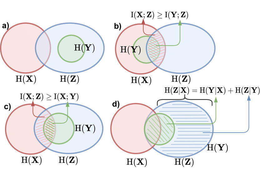
Figure 2: Venn diagram of the transitive information theorem, illustrating interaction between 𝐱𝐱\mathbf{x} and 𝐳𝐳\mathbf{z} given different choices for 𝐲𝐲\mathbf{y}: a)a) 𝐲𝐲\mathbf{y} is random noise; b)b) 𝐲𝐲\mathbf{y} is ground truth; c)c) 𝐲𝐲\mathbf{y} is partially observed ground truth; and d)d) achieved equality.

In practice, our concern is the interaction between 𝐲𝐲\mathbf{y} and 𝐳𝐳\mathbf{z}. The first case is that H(𝐲|𝐱)=0𝐻conditional𝐲𝐱0H(\mathbf{y}|\mathbf{x})=0 (Fig. 2-b)), i.e. 𝐲𝐱𝐲𝐱\mathbf{y}\in\mathbf{x}, then (3) takes simpler form I(𝐱,𝐳)I(𝐲,𝐳)I𝐱𝐳I𝐲𝐳\mathrm{I}(\mathbf{x},\mathbf{z})\geq\mathrm{I}(\mathbf{y},\mathbf{z}), hence, increasing I(𝐲,𝐳)I𝐲𝐳\mathrm{I}(\mathbf{y},\mathbf{z}) directly pushes the lower bound of our target MI. Because 𝐲𝐲\mathbf{y} and 𝐳𝐳\mathbf{z} are much lower dimensions than 𝐱𝐱\mathbf{x}, the computational burden is significantly reduced. In the second case, our question is “Would it be possible to learn latents that contain more information than the groundtruth factors?”, in mathematical sense, it is I(𝐱,𝐳)I(𝐱,𝐲)I𝐱𝐳I𝐱𝐲\mathrm{I}(\mathbf{x},\mathbf{z})\geq\mathrm{I}(\mathbf{x},\mathbf{y}) (Fig. 2-c)). This is proves to be possible when H(𝐲|𝐳)=0𝐻conditional𝐲𝐳0H(\mathbf{y}|\mathbf{z})=0 in which 𝐲𝐳𝐲𝐳\mathbf{y}\subset\mathbf{z} and the latents would absorb all the knowledge about 𝐲𝐲\mathbf{y}, while being free to explore beyond the known manifold. The final case is when the solution for 𝐳𝐳\mathbf{z} is optimal, i.e. equality is achieved in (3). Figure 2-d shows that 𝐳𝐳\mathbf{z} also contains all the information about 𝐲𝐲\mathbf{y}, however, I(𝐱,𝐳)I𝐱𝐳\mathrm{I}(\mathbf{x},\mathbf{z}) is bounded to be equal to I(𝐱,𝐲)I𝐱𝐲\mathrm{I}(\mathbf{x},\mathbf{y}). Additionally, the role of 𝐲𝐲\mathbf{y} could be understood by the offset term H(𝐲)𝐻𝐲-H(\mathbf{y}), i.e. the more information we know about 𝐲𝐲\mathbf{y}, the tighter the bound.

Theorem 2 is an instrument for understanding the relationship between ground truth factors 𝐲𝐲\mathbf{y} and the learned latent 𝐳𝐳\mathbf{z}. Specifically, it shows that there is an infinite number of solutions for learning 𝐳𝐳\mathbf{z} that achieved the same amount of MI with 𝐱𝐱\mathbf{x} as I(𝐱,𝐲)I𝐱𝐲\mathrm{I}(\mathbf{x},\mathbf{y}). Hence, a good representation might not need to be identical to 𝐲𝐲\mathbf{y}, in other words, good representation might not need disentangled factors. In theory, it is desirable to learn a complete factorized representation that each dimension individually associates with a single disentangled factor. In practice, the ground truth factors are often entangled, for instance color can be both represented in the RGB space or HSV space, or one might observe the shadow instead of the shape of an object. Moreover, the ground truth factors aren’t necessary the best representations, e.g. wasting two dimensions modeling x and y-axis for 28×28282828\times 28 images is less efficient than having a single dimension store all 784784784 pixels. As a result, learning an independent mechanism that recombines and reuses representation is more robust to the distribution shift in the context of deep generative model Schölkopf et al. (2021); Montero et al. (2021); Träuble et al. (2020). Since study in Locatello et al. (2019) proves learning such mechanism in an unsupervised manner is infeasible, we focus on the semi-supervised setting which also enables our representation to be controllable by meaningful factors.

3.2 Semi-supervised maximizing mutual information VAE

We observe that certain VAE models have high capacity latents, but they generate meaningless images that seems to be the mixture of fine details from multiple training examples. This is particularly common phenomenon when reducing the strength of regularization term in ELBO even though the reconstructed image is much sharper and a t-SNE plot of the latent space shows strong correlation between the latent codes and the ground truth factors222Additional experiments in the Appendix. We attribute two explanations to the issue: 1) the lack of hierarchy in the representation due to assumed mean field approximation, all representations are learned equally so that there are large amounts of generative combination; 2) the uninformative prior induces a gap between inference and generation which also render the generation uncontrollable. In Bozkurt et al. , the regularization term is decomposed into Iq(𝐱,𝐳)+D𝙺𝙻(q(𝐳)||p(𝐳))\mathrm{I}_{\mathrm{q}}(\mathbf{x},\mathbf{z})+\mathrm{D}_{\mathtt{KL}}({q(\mathbf{z})}||{p(\mathbf{z})}) where q(𝐳)𝑞𝐳q(\mathbf{z}) is the aggregated posterior, the authors show that generalization keep improved despite Iq(𝐱,𝐳)subscriptIq𝐱𝐳\mathrm{I}_{\mathrm{q}}(\mathbf{x},\mathbf{z}) saturated to the maximum value which indicates the importance of “the marginal KL” - D𝙺𝙻(q(𝐳)||p(𝐳))\mathrm{D}_{\mathtt{KL}}({q(\mathbf{z})}||{p(\mathbf{z})}) and the choice of more informative prior.

As a result, we propose SEmi-supervised MAximizing mutual inFOrmation VAE (SemafoVAE) to learn meaningful and controllable prior in semi-supervised manner. Furthermore, the approach is inspired by the “semaphore” concept in computer science, that the information bottleneck in VAE is overcome by an alternative pathway created in the prior that maximize I(𝐲,𝐳)I𝐲𝐳\mathrm{I}(\mathbf{y},\mathbf{z}). Figure 3-c shows the graphical model of our approach in comparison to the conditional M2-VAE Kingma et al. (2014) and capturing characteristic VAE (CCVAE) Joy et al. (2021). Major differences are the assumption regarding the role of partially observed ground truth 𝐲𝐲\mathbf{y} in generating observation 𝐱𝐱\mathbf{x}, whereas Kingma et al. (2014) (Figure 3-a) requires 𝐲𝐲\mathbf{y} to be marginalized in the generation and the role of 𝐲𝐲\mathbf{y} is completely detached from the learned representation. In Joy et al. (2021) (Figure 3-b), the assumption is that the label characteristics should be captured independently and in parallel with the latent style variables. Lastly, SemafoVAE emphasizes the absolute control of the ground truth factors on the latent space, hence, forcing the representation to be a smooth universal transformation among all classes (e.g. the same mechanism should be used to rotate an image of number 0, 1, or 2).

Refer to caption
Figure 3: The graphical models of semi-supervised VAE systems where 𝒫𝒫\mathcal{P} denotes generative model, 𝒬𝒬\mathcal{Q} denotes inference model. a)a) conditional M2 VAE Kingma et al. (2014); b)b) CCVAE Joy et al. (2021); and c)c) the proposed SemafoVAE. d)d) is the implementation of SemafoVAE which consist of two VAEs learned jointly.

3.3 Learning objectives and theoretical justification

In order to construct an objective for the model above, we formulate a lower bound on the model log-likelihood which factors over the supervised 𝒮𝒮\mathcal{S} subset and unsupervised 𝒰𝒰\mathcal{U} subset of data, i.e. p(𝐱,𝐲)=𝐱𝒰p(𝐱)(𝐱,𝐲)𝒮p(𝐱,𝐲)𝑝𝐱𝐲subscriptproduct𝐱𝒰𝑝𝐱subscriptproduct𝐱𝐲𝒮𝑝𝐱𝐲p(\mathbf{x},\mathbf{y})=\prod_{\mathbf{x}\in\mathcal{U}}p(\mathbf{x})\cdot\prod_{(\mathbf{x},\mathbf{y})\in\mathcal{S}}p(\mathbf{x},\mathbf{y}). A detailed derivation for the following ELBOs is in the Appendix A.4, the objective for unsupervised learning and supervised learning are:

logp(𝐱)Eq(𝐳|𝐱)[logp(𝐱|𝐳)]Eq(𝐲|𝐳)[D𝙺𝙻(q(𝐳|𝐱)||p(𝐳|𝐲))]Eq(𝐳|𝐱)[D𝙺𝙻(q(𝐲|𝐳)||p(𝐲))]\log p(\mathbf{x})\geq\mathrm{E}_{q(\mathbf{z}|\mathbf{x})}\big{[}\log p(\mathbf{x}|\mathbf{z})\big{]}-\mathrm{E}_{q(\mathbf{y}|\mathbf{z})}\big{[}\mathrm{D}_{\mathtt{KL}}({q(\mathbf{z}|\mathbf{x})}||{p(\mathbf{z}|\mathbf{y})})\big{]}-\mathrm{E}_{q(\mathbf{z}|\mathbf{x})}\big{[}\mathrm{D}_{\mathtt{KL}}({q(\mathbf{y}|\mathbf{z})}||{p(\mathbf{y})})\big{]} (4)

and

logp(𝐱,𝐲)Eq(𝐳|𝐱)[logp(𝐱|𝐳)]D𝙺𝙻(q(𝐳|𝐱)||p(𝐳|𝐲))+logp(𝐲).\log p(\mathbf{x},\mathbf{y})\geq\mathrm{E}_{q(\mathbf{z}|\mathbf{x})}\big{[}\log p(\mathbf{x}|\mathbf{z})\big{]}-\mathrm{D}_{\mathtt{KL}}({q(\mathbf{z}|\mathbf{x})}||{p(\mathbf{z}|\mathbf{y})})+\log p(\mathbf{y}). (5)

Unlike the approach in Kingma et al. (2014); Joy et al. (2021) which assume that the prior p(𝐲)𝑝𝐲p(\mathbf{y}) is uninformative, we take a more generalized approach. First, 𝐲𝐲\mathbf{y} could take any arbitrary distribution, and second we want its prior distribution to be informative and learnable. As a result, we assume that these factors are independently distributed as the factorized joint distribution: p(𝐲)=y𝒴p(y)𝑝𝐲subscriptproduct𝑦𝒴𝑝𝑦p(\mathbf{y})=\prod_{y\in\mathcal{Y}}p(y) where 𝒴𝒴\mathcal{Y} is our set of partially observed factors.

To this point, maximizing logp(𝐲)𝑝𝐲\log p(\mathbf{y}) is intractable for all possible outcomes in 𝒴𝒴\mathcal{Y}, hence, we utilize additional latent variables 𝐮𝐮\mathbf{u} in order to maximize the ELBO of logp(𝐲)𝑝𝐲\log p(\mathbf{y}). Since 𝐲𝐲\mathbf{y} has smaller number of dimensions, and its true manifold dimension is the number of disentangled factors, we set the number of latent dimensions d𝐮=|𝒴|subscript𝑑𝐮𝒴d_{\mathbf{u}}=|\mathcal{Y}|. ELBO is then,

logp(𝐲)Eq(𝐮|𝐲)[logp(𝐲|𝐮)]D𝙺𝙻(q(𝐮|𝐲)||p(𝐮))=(𝐲,𝐮).\displaystyle\log p(\mathbf{y})\geq\mathrm{E}_{q(\mathbf{u}|\mathbf{y})}\big{[}\log p(\mathbf{y}|\mathbf{u})\big{]}-\mathrm{D}_{\mathtt{KL}}({q(\mathbf{u}|\mathbf{y})}||{p(\mathbf{u})})=\mathcal{E}(\mathbf{y},\mathbf{u}). (6)

Next, we want to minimize the quantity D𝙺𝙻(q(𝐳|𝐱)||p(𝐳||𝐲))\mathrm{D}_{\mathtt{KL}}({q(\mathbf{z}|\mathbf{x})}||{p(\mathbf{z}||\mathbf{y})}) given (6). The principle is in the Theorem 2, as we use 𝐮𝐮\mathbf{u} as an auxiliary (bridge) variable for transferring information between 𝐲𝐲\mathbf{y} and 𝐳𝐳\mathbf{z}, thus we assume the factorization: p(𝐳,𝐲,𝐮)=p(𝐲|𝐮)p(𝐳|𝐮)p(𝐮)𝑝𝐳𝐲𝐮𝑝conditional𝐲𝐮𝑝conditional𝐳𝐮𝑝𝐮p(\mathbf{z},\mathbf{y},\mathbf{u})=p(\mathbf{y}|\mathbf{u})p(\mathbf{z}|\mathbf{u})p(\mathbf{u}), so that:

D𝙺𝙻(q(𝐳|𝐱)||p(𝐳||𝐲))\displaystyle\mathrm{D}_{\mathtt{KL}}({q(\mathbf{z}|\mathbf{x})}||{p(\mathbf{z}||\mathbf{y})}) =Eq(𝐳|𝐱)[logq(𝐳|𝐱)]Eq(𝐳|𝐱)[logup(𝐳,𝐲,𝐮)du]applying a lower bound+Eq(𝐳|𝐱)[logp(𝐲)]absentsubscriptE𝑞conditional𝐳𝐱delimited-[]𝑞conditional𝐳𝐱subscriptsubscriptE𝑞conditional𝐳𝐱delimited-[]subscript𝑢𝑝𝐳𝐲𝐮differential-d𝑢applying a lower boundsubscriptE𝑞conditional𝐳𝐱delimited-[]𝑝𝐲\displaystyle=\mathrm{E}_{q(\mathbf{z}|\mathbf{x})}\big{[}\log q(\mathbf{z}|\mathbf{x})\big{]}-\underbrace{\mathrm{E}_{q(\mathbf{z}|\mathbf{x})}\big{[}\log\int_{u}p(\mathbf{z},\mathbf{y},\mathbf{u})\mathrm{d}u\big{]}}_{\text{applying a lower bound}}+\mathrm{E}_{q(\mathbf{z}|\mathbf{x})}\big{[}\log p(\mathbf{y})\big{]} (7)
Eq(𝐳|𝐱)q(𝐮|𝐲)[D𝙺𝙻(q(𝐳|𝐱)||p(q(𝐳|𝐮))](𝐲,𝐮)+logp(𝐲),\displaystyle\leq\mathrm{E}_{q(\mathbf{z}|\mathbf{x})q(\mathbf{u}|\mathbf{y})}\big{[}\mathrm{D}_{\mathtt{KL}}({q(\mathbf{z}|\mathbf{x})}||{p(q(\mathbf{z}|\mathbf{u})})\big{]}-\mathcal{E}(\mathbf{y},\mathbf{u})+\log p(\mathbf{y}),

where (𝐲,𝐮)𝐲𝐮\mathcal{E}(\mathbf{y},\mathbf{u}) is defined by (6). In other words, we could minimize D𝙺𝙻(q(𝐳|𝐱)||p(𝐳||𝐲))\mathrm{D}_{\mathtt{KL}}({q(\mathbf{z}|\mathbf{x})}||{p(\mathbf{z}||\mathbf{y})}) by minimizing its upper bound, and the role of 𝐮𝐮\mathbf{u} is beautifully justified when we substitute (7) to (4) and (5) which eliminates the need for maximizing the intractable evidence logp(𝐲)𝑝𝐲\log p(\mathbf{y}) and replaces 𝐲𝐲\mathbf{y} by the tractable latent 𝐮𝐮\mathbf{u} in all of our KL divergence terms. As a result, the final unsupervised and supervised ELBOs for SemafoVAE are:

𝚄(𝐱,𝐳)subscript𝚄𝐱𝐳\displaystyle\mathcal{E}_{\mathtt{U}}(\mathbf{x},\mathbf{z}) =Eq(𝐳|𝐱)[logp(𝐱|𝐳)]Eq(𝐳,𝐲,𝐮|𝐱)[D𝙺𝙻(q(𝐳|𝐱)||p(𝐳|𝐮))]+\displaystyle=\mathrm{E}_{q(\mathbf{z}|\mathbf{x})}\big{[}\log p(\mathbf{x}|\mathbf{z})\big{]}-\mathrm{E}_{q(\mathbf{z},\mathbf{y},\mathbf{u}|\mathbf{x})}\big{[}\mathrm{D}_{\mathtt{KL}}({q(\mathbf{z}|\mathbf{x})}||{p(\mathbf{z}|\mathbf{u})})\big{]}+ (8)
Eq(𝐲|𝐳)[(𝐲,𝐮)]Eq(𝐳|𝐱)[logq(𝐲|𝐳)]subscriptE𝑞conditional𝐲𝐳delimited-[]𝐲𝐮subscriptE𝑞conditional𝐳𝐱delimited-[]𝑞conditional𝐲𝐳\displaystyle\quad\quad\mathrm{E}_{q(\mathbf{y}|\mathbf{z})}\big{[}\mathcal{E}(\mathbf{y},\mathbf{u})\big{]}-\mathrm{E}_{q(\mathbf{z}|\mathbf{x})}\big{[}\log q(\mathbf{y}|\mathbf{z})\big{]}

and

𝚂(𝐱,𝐲,𝐳)subscript𝚂𝐱𝐲𝐳\displaystyle\mathcal{E}_{\mathtt{S}}(\mathbf{x},\mathbf{y},\mathbf{z}) =Eq(𝐳|𝐱)[logp(𝐱|𝐳)]Eq(𝐳,𝐮|𝐱,𝐲)[D𝙺𝙻(q(𝐳|𝐱)||p(𝐳|𝐮))]+(𝐲,𝐮).\displaystyle=\mathrm{E}_{q(\mathbf{z}|\mathbf{x})}\big{[}\log p(\mathbf{x}|\mathbf{z})\big{]}-\mathrm{E}_{q(\mathbf{z},\mathbf{u}|\mathbf{x},\mathbf{y})}\big{[}\mathrm{D}_{\mathtt{KL}}({q(\mathbf{z}|\mathbf{x})}||{p(\mathbf{z}|\mathbf{u})})\big{]}+\mathcal{E}(\mathbf{y},\mathbf{u}). (9)

These two objectives are combined into the final ELBO for optimization 𝚂𝚎𝚖𝚊𝚏𝚘𝚅𝙰𝙴=𝚄(𝐱,𝐳)+𝚂(𝐱,𝐲,𝐳)subscript𝚂𝚎𝚖𝚊𝚏𝚘𝚅𝙰𝙴subscript𝚄𝐱𝐳subscript𝚂𝐱𝐲𝐳\mathcal{E}_{\mathtt{SemafoVAE}}=\mathcal{E}_{\mathtt{U}}(\mathbf{x},\mathbf{z})+\mathcal{E}_{\mathtt{S}}(\mathbf{x},\mathbf{y},\mathbf{z}).

Lemma 3.

For the factorized joint distribution p(𝐱,𝐲,𝐳)=pθ(𝐱|𝐳)pψ(𝐳|𝐲)p(𝐲)𝑝𝐱𝐲𝐳subscript𝑝𝜃conditional𝐱𝐳subscript𝑝𝜓conditional𝐳𝐲𝑝𝐲p(\mathbf{x},\mathbf{y},\mathbf{z})=p_{\theta}(\mathbf{x}|\mathbf{z})p_{\psi}(\mathbf{z}|\mathbf{y})p(\mathbf{y}), and the assumed inference model q(𝐱,𝐲,𝐳)=qτ(𝐲|𝐳)qϕ(𝐳|𝐱)q𝒟(𝐱)𝑞𝐱𝐲𝐳subscript𝑞𝜏conditional𝐲𝐳subscript𝑞italic-ϕconditional𝐳𝐱subscript𝑞𝒟𝐱q(\mathbf{x},\mathbf{y},\mathbf{z})=q_{\tau}(\mathbf{y}|\mathbf{z})q_{\phi}(\mathbf{z}|\mathbf{x})q_{\mathcal{D}}(\mathbf{x}). Then, there exists the solution parameters {θ,ψ,τ,ϕ}𝜃𝜓𝜏italic-ϕ\{\theta,\psi,\tau,\phi\} for SemafoVAE, such that the mutual information between the generated example and the ground truth factor Ip(𝐱,𝐲)subscriptIp𝐱𝐲\mathrm{I}_{\mathrm{p}}(\mathbf{x},\mathbf{y}) is maximized.

The lemma is proved using Barber and Agakov (2003) lemma to show that given enough data, optimal optimizer and constrained entropy Hp(𝐳|𝐲)0subscriptHpconditional𝐳𝐲0\mathrm{H}_{\mathrm{p}}(\mathbf{\mathbf{z}|\mathbf{y}})\geq 0, SemafoVAE maximizes the lower bound of Ip(𝐱,𝐳)subscriptIp𝐱𝐳\mathrm{I}_{\mathrm{p}}(\mathbf{x},\mathbf{z}) and Ip(𝐳,𝐲)subscriptIp𝐳𝐲\mathrm{I}_{\mathrm{p}}(\mathbf{z},\mathbf{y}), and according to Theorem 2, maximizing the lower bound of Ip(𝐱,𝐲)subscriptIp𝐱𝐲\mathrm{I}_{\mathrm{p}}(\mathbf{x},\mathbf{y}). Full detailed proof is in the Appendix A.6. We expect the objective of 𝚂𝚎𝚖𝚊𝚏𝚘𝚅𝙰𝙴subscript𝚂𝚎𝚖𝚊𝚏𝚘𝚅𝙰𝙴\mathcal{E}_{\mathtt{SemafoVAE}} to improve the MI of the generated examples and the ground truth factors, i.e. generating relevant example using the prior. The implementation of SemafoVAE is described Figure 3-d which consists of two VAEs optimized jointly. The reconstruction VAE learns the posterior q(𝐳|𝐱)𝑞conditional𝐳𝐱q(\mathbf{z}|\mathbf{x}) as in the original VAE framework Kingma and Welling (2014), while the controller VAE learns the controllable prior p(𝐳|𝐮)𝑝conditional𝐳𝐮p(\mathbf{z}|\mathbf{u}). The training algorithm for SemafoVAE is specified in Appendix A.7. It is also notable that our approach operates on the prior distribution, hence, it could be integrated to any existing VAE model as an extension.

4 Related works

Richer connection between 𝐳𝐳\mathbf{z} and 𝐱𝐱\mathbf{x} would increase the capacity of VAE by allowing the modeling of more complicated factors in the generation process. One possibility is to introduce auxiliary variables 𝐚𝐚\mathbf{a} that factorizes the approximated posterior distribution into q(𝐳|𝐱)=aq(𝐳|𝐚,𝐱)q(𝐚|𝐱)da𝑞conditional𝐳𝐱subscript𝑎𝑞conditional𝐳𝐚𝐱𝑞conditional𝐚𝐱differential-d𝑎q(\mathbf{z}|\mathbf{x})=\int_{a}q(\mathbf{z}|\mathbf{a},\mathbf{x})q(\mathbf{a}|\mathbf{x})\mathrm{d}a, as a result, enabling complicated covariance structure in q(𝐳|𝐱)𝑞conditional𝐳𝐱q(\mathbf{z}|\mathbf{x})  Maaløe et al. (2016). Similar idea could be found in the hierarchical latent models Sønderby et al. (2016); Maaløe et al. (2019); Child (2021) which stack multiple stochastic units to form hierarchical structures qϕ(𝐳L|𝐱)=zqϕ(𝐳L|𝐳<L,𝐱)qϕ(𝐳<L|𝐱)𝑑zsubscript𝑞italic-ϕconditionalsubscript𝐳𝐿𝐱subscript𝑧subscript𝑞italic-ϕconditionalsubscript𝐳𝐿subscript𝐳absent𝐿𝐱subscript𝑞italic-ϕconditionalsubscript𝐳absent𝐿𝐱differential-d𝑧q_{\phi}(\mathbf{z}_{L}|\mathbf{x})=\int_{z}q_{\phi}(\mathbf{z}_{L}|\mathbf{z}_{<L},\mathbf{x})q_{\phi}(\mathbf{z}_{<L}|\mathbf{x})dz. The learned representation exhibits multiple levels of abstraction, and it also improves the quality of generated images.

Other directions focus on having more powerful posterior distribution Kingma et al. (2016); Davidson et al. (2019) or more accurate prior distribution Chen et al. (2017); Tomczak and Welling (2018). The approximated posterior can be for example used to capture clustering via mixture of Gaussian Nalisnick et al. (2016), or encapsulate geometric patterns via hyper-spherical distribution Davidson et al. (2019). Optimal choice of prior can be approximated without being overfitted to the training data, the result is an empirical mixture of priors that utilizes mixtures of pseudo-inputs {𝐮1,,𝐮K}subscript𝐮1subscript𝐮𝐾\{\mathbf{u}_{1},...,\mathbf{u}_{K}\} Tomczak and Welling (2018). However, relying on the pseudo-inputs for prior would introduce unnecessary inductive bias to 𝐳𝐳\mathbf{z}, which consequently limits its capacity to explore the data manifold. In Kumar et al. (2018) it was shown that disentangled representation needs disentangled prior, and by placing constraints on the covariance structure, we could push the posterior closer to the disentangled prior.

To the best of our knowledge, learning a complete disentangled factors in unsupervised fashion is infeasible Locatello et al. (2019); Montero et al. (2021). Even though there exist successes in incorporating weak supervision that facilitates disentanglement Shu et al. (2019); Locatello et al. (2020), this form of supervision might still be too far reach for real world setting since it requires labels for every example. The goal is to achieve disentanglement and controllability via semi-supervised learning with minimal labeling. Similar approaches in Kingma et al. (2014); Maaløe et al. (2016); Joy et al. (2021) aim to learn FOVs (styles) and labeling classes in separation, however, our assumption differs that the discovered factors are given by prior knowledge about the classes, thus, enabling multiple levels of hierarchy in the prior distribution.

5 Experiments and results

Table 1: The baselines system and their improvement compared to the vanilla VAE: D𝐷D for disentanglement, L𝐿L for reconstruction log-likelihood and C𝐶C for controllability of the latent representation. UNS is unsupervised methods and SSL is semi-supervised methods.

Group Method Improvement D𝐷D L𝐿L C𝐶C UNS BetaVAE Higgins et al. (2017) GammaVAE Rezende and Viola (2018) FactorVAE Kim and Mnih (2018) HierarchicalVAE Kingma et al. (2016) SSL M2 Kingma et al. (2014) CCVAE Joy et al. (2021) SemafoVAE SemafoHVAE

SemafoVAE is compared to a wide range of different approaches from unsupervised to semi-supervised Table 1. All methods are our reimplementations, and the performance closely match to the description in the original papers. The exception is GammaVAE which is our modification of Bozkurt et al. that places extra weight to the reconstruction term of ELBO to specifically improve the log-likelihood. Since SemafoVAE work well as an extension to any existing VAE, we also introduce the Semafo-HierarchicalVAE which is the combination of SemafoVAE prior and hierarchical latent variables model Kingma et al. (2016).

We utilize the three standard benchmark datasets: MNIST LeCun et al. (2010), Fashion MNIST (F-MNIST)Xiao et al. (2017) and Shapes3D Burgess and Kim (2018). The percent of labelling examples for semi-supervision scenarios are 0.0040.0040.004, 0.010.010.01 and 0.10.10.1 corresponding to the three datasets. The multi-class labels in the first two datasets are treated as ground truth factors while the discretized factors are used for Shapes3D. We use the benchmark architectures from Locatello et al. (2019), a Bernoulli distribution is fitted for each pixel and the latent variables are multivariate diagonal normal, and Gumbel-Softmax Jang et al. (2016) for parameterizing every individual factor y𝑦y. The experimental details can be found in Appendix.

5.1 Quantitative evaluation

The SemafoVAE shows consistent improvement to the baseline methods in all three benchmarks, and it is the only semi-supervised method that improves both the generation and the quality of the representation according to the FID and DCI scores. With only two methods have better test log-likelihood (GammaVAE and HVAE) in certain cases, however, both of these methods achieve much lower FID for generated data and DCI for learned representation. A Semafo prior applied to either the vanilla VAE or the HVAE both show significant improvement. Among the semi-supervised approaches, our methods achieve the highest scores in all benchmarks.

Table 2: From left to right: reconstruction log-likelihood (higher is better), FID (Heusel et al. (2017)) of random generated samples (lower is better), and the disentanglement, informativeness, completeness (DCI Eastwood and Williams (2018)) score between the learned representation and the ground truth factors (higher is better). All scores are calculated using test set. Since there are no ground truth factors for MNIST and F-MNIST, the given DCI score is the accuracy of downstream classifier. denotes hierarchical latent models.

Reconstruction Log-likelihood Fréchet Inception Distance DCI score Model MNIST F-MNIST Shapes3D MNIST F-MNIST Shapes3D MNIST F-MNIST Shapes3D Unsupervised methods VAE -71.27 -222.07 -3464.40 48.24 97.52 74.57 89.80 78.90 64.82 BetaVAE -142.81 -258.83 -3492.65 107.33 159.69 49.89 87.25 78.05 58.56 GammaVAE -54.95 -206.04 -3456.99 51.31 119.43 141.33 89.75 81.30 48.89 FactorVAE -79.37 -226.64 -3470.09 46.87 95.63 115.24 85.55 78.15 63.11 HVAE -65.84 -213.50 -3451.54 48.68 85.99 82.20 92.65 82.50 69.03 Semi-supervised methods M2 -83.81 -231.80 -3464.79 64.50 105.80 81.63 47.25 59.60 24.42 CCVAE -80.53 -228.63 -3473.60 47.82 117.44 115.17 91.65 81.50 80.32 SemafoVAE -56.02 -212.54 -3457.03 45.57 92.28 93.63 90.30 81.40 80.88 SemafoHVAE -52.96 -209.07 -3451.80 42.97 70.61 62.36 90.60 84.05 82.62

5.2 Controlling and disentangling of the representation

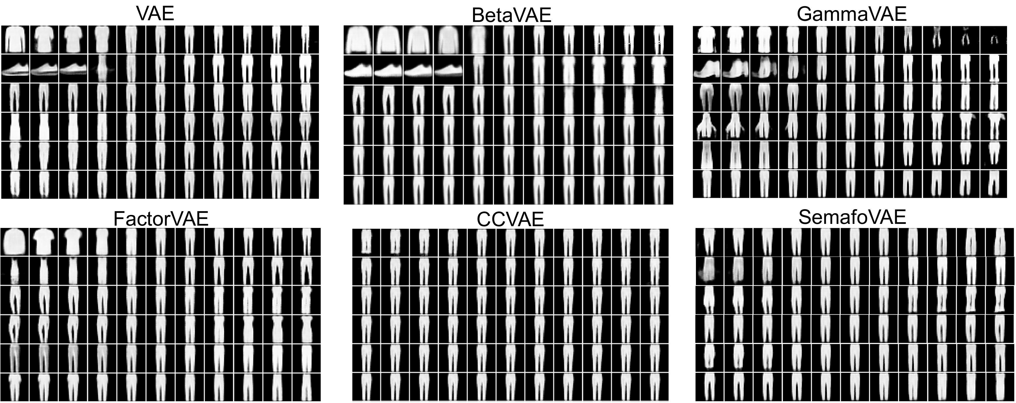
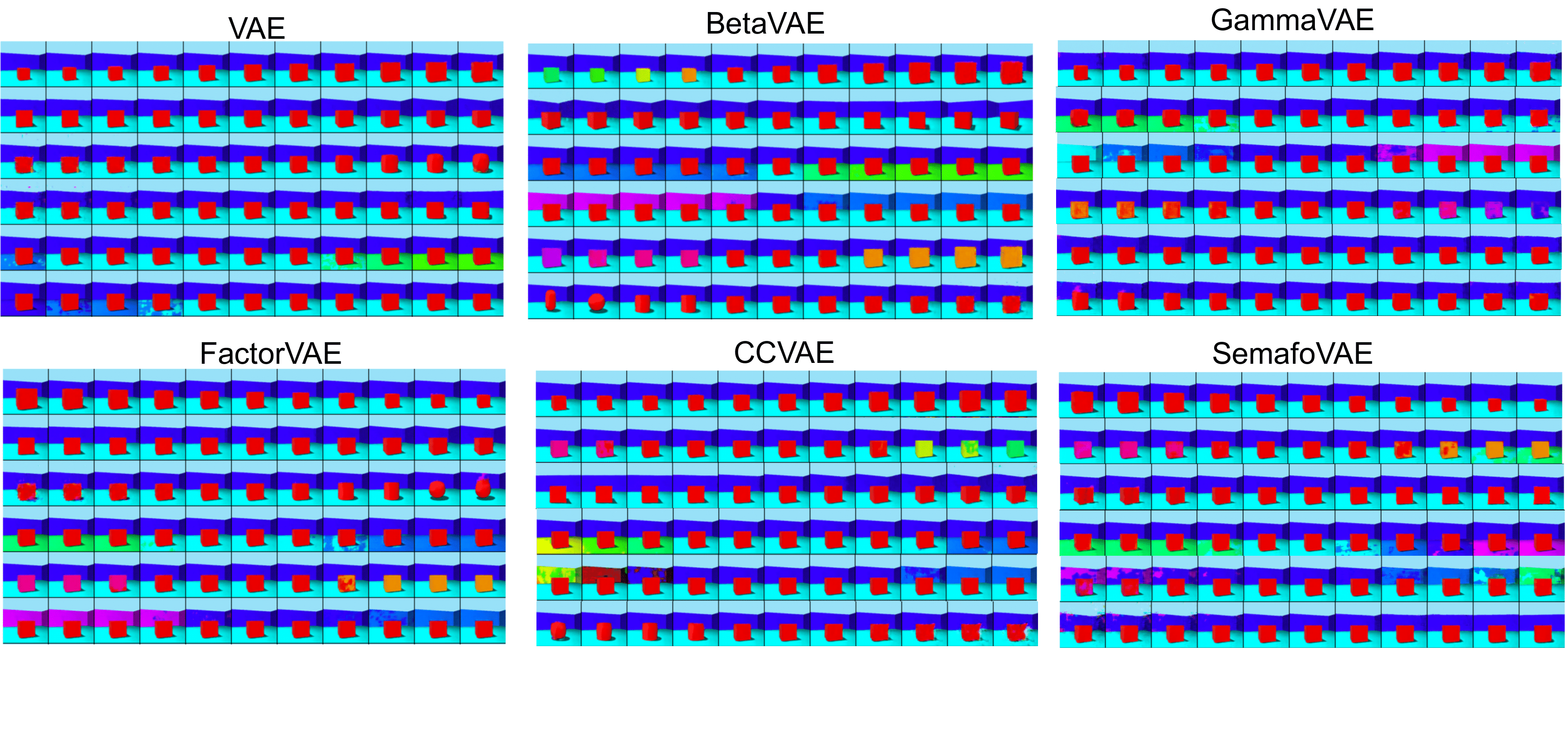
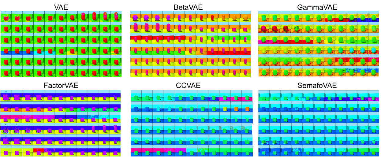
It is notable that the only existing method that focus on controllability of latent representation is CCVAE Joy et al. (2021), however, this method only partially control the latent units. Figure 4 (left) shows that SemafoVAE has perfect control of all factors in generation. Since our method learn an informative prior, it is capable of prior traverse along with the conventional method of posterior traverse. Figure 4 (middle and right) show that the algorithm has been able to learn smooth traverse of meaningful factors in both of its prior and posterior. The implication is that SemafoVAE can do meaningful intervention of existing attributes, and also supports discovering new combination by traversing completely random prior. More details of the traverse among different VAEs are provided in the Appendix.

Refer to caption
Figure 4: Left: Random examples generated from the prior conditioned so that only the shapes and the object hue is varied. Middle: Given a shirt (top row) and a dress (bottom row), SemafoVAE learns a conditional prior p(𝐳|𝐮,𝐲)𝑝conditional𝐳𝐮𝐲p(\mathbf{z}|\mathbf{u},\mathbf{y}) that support smooth traverse in the prior. Right: posterior traverse of a given examples.

6 Conclusion

In order to enable practical application, not only generative model has to learn an efficient representation that is hierarchical and disentangled, but also realizes a mechanism that recombines the learned representation in a meaningful way. We present a novel approach that enables VAE to achieve all the proposed criteria. Moreover, we develop the mutual information maximization theory that supports the design of our Semafo prior which could be integrated into the existing VAE framework. The prior achieve controllability via adding a minimal amount of supervision using a semi-supervised paradigm. This assumption of variables’ hierarchy indirectly introduces inductive bias to the posterior without restricting its ability to explore the factor characteristics. The result is a great degree of controllability while retaining meaningful disentangled latent representation. Since we have successfully integrated SemafoVAE to Hierarchical VAE, our future would focus on scaling up this architecture to achieve controllable realistic image generation.

References

  • Alemi et al. [2017] Alexander A. Alemi, Ben Poole, Ian Fischer, Joshua V. Dillon, Rif A. Saurous, and Kevin Murphy. Fixing a Broken ELBO. arXiv:1711.00464 [cs, stat], November 2017.
  • Alemi et al. [2019] Alexander A. Alemi, Ian Fischer, Joshua V. Dillon, and Kevin Murphy. Deep Variational Information Bottleneck. arXiv:1612.00410 [cs, math], October 2019.
  • Barber and Agakov [2003] David Barber and Felix Agakov. The IM algorithm: A variational approach to information maximization. In Proceedings of the 16th International Conference on Neural Information Processing Systems, NIPS’03, pages 201–208, Cambridge, MA, USA, 2003. MIT Press.
  • Bengio et al. [2014] Y. Bengio, A. Courville, and P. Vincent. Representation Learning: A Review and New Perspectives. IEEE Transactions on Pattern Analysis and Machine Intelligence, 35(8):1798–1828, 2014.
  • Bishop [2006] Christopher M. Bishop. Pattern Recognition and Machine Learning. Information Science and Statistics. Springer, New York, 2006. ISBN 978-0-387-31073-2.
  • [6] Alican Bozkurt, Dana H Brooks, Babak Esmaeili, and Jean-Baptiste Tristan. Rate-Regularization and Generalization in VAEs. page 11.
  • Burgess and Kim [2018] Chris Burgess and Hyunjik Kim. 3d shapes dataset. https://github.com/deepmind/3dshapes-dataset/, 2018.
  • Burgess et al. [2018] Christopher P. Burgess, Irina Higgins, Arka Pal, Loïc Matthey, Nick Watters, Guillaume Desjardins, and Alexander Lerchner. Understanding disentangling in β𝛽\beta-VAE. CoRR, abs/1804.03599, 2018.
  • Chen et al. [2017] Xi Chen, Diederik P. Kingma, Tim Salimans, Yan Duan, Prafulla Dhariwal, John Schulman, Ilya Sutskever, and Pieter Abbeel. Variational Lossy Autoencoder. ICLR, March 2017.
  • Child [2021] Rewon Child. Very deep {}VAE{}s generalize autoregressive models and can outperform them on images. In International Conference on Learning Representations, 2021.
  • Cover and Thomas [2006] Thomas M. Cover and Joy A. Thomas. Elements of Information Theory (Wiley Series in Telecommunications and Signal Processing). Wiley-Interscience, USA, 2006. ISBN 0-471-24195-4.
  • Dai and Wipf [2019] Bin Dai and David Wipf. Diagnosing and Enhancing VAE Models. arXiv:1903.05789 [cs, stat], March 2019.
  • Dai et al. [2019] Bin Dai, Ziyu Wang, and David Wipf. The Usual Suspects? Reassessing Blame for VAE Posterior Collapse. arXiv:1912.10702 [cs, stat], December 2019.
  • Davidson et al. [2019] Tim R Davidson, Jakub M Tomczak, and Efstratios Gavves. Increasing Expressivity of a Hyperspherical VAE. Bayesian Deep Learning, NIPS, page 8, 2019.
  • Eastwood and Williams [2018] Cian Eastwood and Christopher K. I. Williams. A framework for the quantitative evaluation of disentangled representations. In International Conference on Learning Representations, 2018.
  • Goodfellow [2017] Ian Goodfellow. NIPS 2016 Tutorial: Generative Adversarial Networks. arXiv:1701.00160 [cs], April 2017.
  • Goodfellow et al. [2014] Ian Goodfellow, Jean Pouget-Abadie, Mehdi Mirza, Bing Xu, David Warde-Farley, Sherjil Ozair, Aaron Courville, and Yoshua Bengio. Generative adversarial nets. In Z. Ghahramani, M. Welling, C. Cortes, N. Lawrence, and K. Q. Weinberger, editors, Advances in Neural Information Processing Systems, volume 27, pages 2672–2680. Curran Associates, Inc., 2014.
  • Havtorn et al. [2021] Jakob D. Havtorn, Jes Frellsen, Søren Hauberg, and Lars Maaløe. Hierarchical VAEs know what they don’t know. CoRR, abs/2102.08248, 2021.
  • He et al. [2019] Junxian He, Daniel Spokoyny, Graham Neubig, and Taylor Berg-Kirkpatrick. Lagging inference networks and posterior collapse in variational autoencoders. In International Conference on Learning Representations, 2019.
  • Heusel et al. [2017] Martin Heusel, Hubert Ramsauer, Thomas Unterthiner, Bernhard Nessler, and Sepp Hochreiter. GANs trained by a two time-scale update rule converge to a local nash equilibrium. In Proceedings of the 31st International Conference on Neural Information Processing Systems, NIPS’17, pages 6629–6640, Red Hook, NY, USA, 2017. Curran Associates Inc. ISBN 978-1-5108-6096-4.
  • Higgins et al. [2017] Irina Higgins, Loic Matthey, Arka Pal, and et al. Beta-VAE: Learning Basic Visual Concepts with a Constrained Variational Framework. ICLR, 2017.
  • Higgins et al. [2018] Irina Higgins, Nicolas Sonnerat, Loic Matthey, Arka Pal, Christopher P Burgess, Matko Bošnjak, Murray Shanahan, Matthew Botvinick, Demis Hassabis, and Alexander Lerchner. SCAN: Learning hierarchical compositional visual concepts. In International Conference on Learning Representations, 2018.
  • Hoffman and Johnson [2016] Matthew D Hoffman and Matthew J Johnson. ELBO surgery: Yet another way to carve up the variational evidence lower bound. NIPS Workshop on Advances in Approximate Bayesian Inference, page 4, 2016.
  • Jang et al. [2016] Eric Jang, Shixiang Gu, and Ben Poole. Categorical Reparameterization with Gumbel-Softmax. arXiv:1611.01144 [cs, stat], November 2016.
  • Joy et al. [2021] Tom Joy, Sebastian Schmon, Philip Torr, Siddharth N, and Tom Rainforth. Capturing label characteristics in {}VAE{}s. In International Conference on Learning Representations, 2021.
  • Karras et al. [2018] Tero Karras, Timo Aila, Samuli Laine, and Jaakko Lehtinen. Progressive growing of GANs for improved quality, stability, and variation. In International Conference on Learning Representations, 2018. URL https://openreview.net/forum?id=Hk99zCeAb.
  • Kim and Mnih [2018] Hyunjik Kim and Andriy Mnih. Disentangling by factorising. volume 80 of Proceedings of Machine Learning Research, pages 2649–2658, Stockholmsmässan, Stockholm Sweden, July 2018. PMLR.
  • Kingma and Ba [2017] Diederik P. Kingma and Jimmy Ba. Adam: A Method for Stochastic Optimization. arXiv:1412.6980 [cs], January 2017.
  • Kingma and Welling [2014] Diederik P. Kingma and Max Welling. Auto-Encoding Variational Bayes. In 2nd International Conference on Learning Representations, ICLR 2014, Banff, AB, Canada, April 14-16, 2014, Conference Track Proceedings, 2014.
  • Kingma et al. [2014] Durk P Kingma, Shakir Mohamed, Danilo Jimenez Rezende, and Max Welling. Semi-supervised learning with deep generative models. In Z. Ghahramani, M. Welling, C. Cortes, N. Lawrence, and K. Q. Weinberger, editors, Advances in Neural Information Processing Systems, volume 27, pages 3581–3589. Curran Associates, Inc., 2014.
  • Kingma et al. [2016] Durk P Kingma, Tim Salimans, Rafal Jozefowicz, Xi Chen, Ilya Sutskever, and Max Welling. Improved variational inference with inverse autoregressive flow. In D. Lee, M. Sugiyama, U. Luxburg, I. Guyon, and R. Garnett, editors, Advances in Neural Information Processing Systems, volume 29, pages 4743–4751. Curran Associates, Inc., 2016.
  • Kumar et al. [2018] Abhishek Kumar, Prasanna Sattigeri, and Avinash Balakrishnan. Variational Inference of Disentangled Latent Concepts from Unlabeled Observations. In International Conference on Learning Representations, 2018.
  • LeCun et al. [2010] Yann LeCun, Corinna Cortes, and CJ Burges. Mnist handwritten digit database. ATT Labs [Online]. Available: http://yann.lecun.com/exdb/mnist, 2, 2010.
  • Locatello et al. [2019] Francesco Locatello, Stefan Bauer, Mario Lučić, Gunnar Rätsch, Sylvain Gelly, Bernhard Schölkopf, and Olivier Frederic Bachem. Challenging Common Assumptions in the Unsupervised Learning of Disentangled Representations. In International Conference on Machine Learning, 2019.
  • Locatello et al. [2020] Francesco Locatello, Ben Poole, Gunnar Rätsch, Bernhard Schölkopf, Olivier Bachem, and Michael Tschannen. Weakly-Supervised Disentanglement Without Compromises. arXiv:2002.02886 [cs, stat], June 2020.
  • Lucas et al. [2019] James Lucas, George Tucker, Roger Grosse, and Mohammad Norouzi. Understanding Posterior Collapse in Generative Latent Variable Models. ICLR, March 2019.
  • Maaløe et al. [2016] Lars Maaløe, Casper Kaae Sønderby, Søren Kaae Sønderby, and Ole Winther. Auxiliary Deep Generative Models. arXiv:1602.05473 [cs, stat], June 2016.
  • Maaløe et al. [2019] Lars Maaløe, Marco Fraccaro, Valentin Liévin, and Ole Winther. BIVA  A very deep hierarchy of latent variables for generative modeling. In NeurIPS, pages 6548–6558, 2019.
  • Meilă [2003] Marina Meilă. Comparing clusterings by the variation of information. In Bernhard Schölkopf and Manfred K. Warmuth, editors, Learning Theory and Kernel Machines, pages 173–187, Berlin, Heidelberg, 2003. Springer Berlin Heidelberg. ISBN 978-3-540-45167-9.
  • Montero et al. [2021] Milton Llera Montero, Casimir JH Ludwig, Rui Ponte Costa, Gaurav Malhotra, and Jeffrey Bowers. The role of disentanglement in generalisation. In International Conference on Learning Representations, 2021.
  • Nakkiran et al. [2019] Preetum Nakkiran, Gal Kaplun, Yamini Bansal, Tristan Yang, Boaz Barak, and Ilya Sutskever. Deep Double Descent: Where Bigger Models and More Data Hurt. arXiv:1912.02292 [cs, stat], December 2019.
  • Nalisnick et al. [2016] Eric Nalisnick, Lars Hertel, and Padhraic Smyth. Approximate Inference for Deep Latent Gaussian Mixtures. Bayesian Deep Learning, NIPS, page 4, 2016.
  • Qiao et al. [2019] Jie Qiao, Zijian Li, Boyan Xu, Ruichu Cai, and Kun Zhang. Disentanglement Challenge: From Regularization to Reconstruction. arXiv:1912.00155 [cs, stat], November 2019.
  • Rezende and Viola [2018] Danilo Jimenez Rezende and Fabio Viola. Taming VAEs. arXiv:1810.00597 [cs, stat], October 2018.
  • Schölkopf et al. [2021] Bernhard Schölkopf, Francesco Locatello, Stefan Bauer, Nan Rosemary Ke, Nal Kalchbrenner, Anirudh Goyal, and Yoshua Bengio. Toward causal representation learning. Proceedings of the IEEE, pages 1–23, 2021. doi: 10.1109/JPROC.2021.3058954.
  • Shu et al. [2019] Rui Shu, Yining Chen, Abhishek Kumar, Stefano Ermon, and Ben Poole. Weakly Supervised Disentanglement with Guarantees. arXiv:1910.09772 [cs, stat], October 2019.
  • Sønderby et al. [2016] Casper Kaae Sønderby, Tapani Raiko, Lars Maaløe, Søren Kaae Sønderby, and Ole Winther. Ladder variational autoencoders. In D. Lee, M. Sugiyama, U. Luxburg, I. Guyon, and R. Garnett, editors, Advances in Neural Information Processing Systems, volume 29, pages 3738–3746. Curran Associates, Inc., 2016.
  • Tishby et al. [1999] Naftali Tishby, Fernando C. Pereira, and William Bialek. The information bottleneck method. In Proc. of the 37-Th Annual Allerton Conference on Communication, Control and Computing, pages 368–377, 1999.
  • Tomczak and Welling [2018] Jakub M. Tomczak and Max Welling. VAE with a VampPrior. arXiv:1705.07120 [cs, stat], February 2018.
  • Träuble et al. [2020] Frederik Träuble, Elliot Creager, Niki Kilbertus, Anirudh Goyal, Francesco Locatello, Bernhard Schölkopf, and Stefan Bauer. Is independence all you need? on the generalization of representations learned from correlated data. CoRR, abs/2006.07886, 2020. URL https://arxiv.org/abs/2006.07886.
  • Vahdat and Kautz [2020] Arash Vahdat and Jan Kautz. NVAE: A deep hierarchical variational autoencoder. In H. Larochelle, M. Ranzato, R. Hadsell, M. F. Balcan, and H. Lin, editors, Advances in Neural Information Processing Systems, volume 33, pages 19667–19679. Curran Associates, Inc., 2020.
  • Xiao et al. [2017] Han Xiao, Kashif Rasul, and Roland Vollgraf. Fashion-mnist: a novel image dataset for benchmarking machine learning algorithms, 2017.

Appendix A Appendix

A.1 Proof for Lemma 1: Rethinking the ELBO

Given the following factorization: qϕ(𝐱,𝐳)=qϕ(𝐳|𝐱)q𝒟(𝐱)subscript𝑞italic-ϕ𝐱𝐳subscript𝑞italic-ϕconditional𝐳𝐱subscript𝑞𝒟𝐱q_{\phi}(\mathbf{x},\mathbf{z})=q_{\phi}(\mathbf{z}|\mathbf{x})q_{\mathcal{D}}(\mathbf{x}) and pθ(𝐱,𝐳)=pθ(𝐱|𝐳)p(𝐳)subscript𝑝𝜃𝐱𝐳subscript𝑝𝜃conditional𝐱𝐳𝑝𝐳p_{\theta}(\mathbf{x},\mathbf{z})=p_{\theta}(\mathbf{x}|\mathbf{z})p(\mathbf{z})

By definition in Kingma and Welling [2014], the ELBO is

(𝒟,ϕ,θ)𝒟italic-ϕ𝜃\displaystyle\mathcal{E}(\mathcal{D},\phi,\theta) =Eq𝒟(𝐱)[Eqϕ(𝐳|𝐱)[logpθ(𝐱|𝐳)]D𝙺𝙻(qϕ(𝐳|𝐱)||p(𝐳))]\displaystyle=\mathrm{E}_{q_{\mathcal{D}}(\mathbf{x})}\bigg{[}\mathrm{E}_{q_{\phi}(\mathbf{z}|\mathbf{x})}\big{[}\mathrm{log}p_{\theta}(\mathbf{x}|\mathbf{z})\big{]}-\mathrm{D}_{\mathtt{KL}}({q_{\phi}(\mathbf{z}|\mathbf{x})}||{p(\mathbf{z})})\bigg{]} (10)
=Eqϕ(𝐱,𝐳)[logpθ(𝐱|𝐳)p(𝐳)qϕ(𝐳|𝐱)]absentsubscriptEsubscript𝑞italic-ϕ𝐱𝐳delimited-[]logsubscript𝑝𝜃conditional𝐱𝐳𝑝𝐳subscript𝑞italic-ϕconditional𝐳𝐱\displaystyle=\mathrm{E}_{q_{\phi}(\mathbf{x},\mathbf{z})}\bigg{[}\mathrm{log}\frac{p_{\theta}(\mathbf{x}|\mathbf{z})p(\mathbf{z})}{q_{\phi}(\mathbf{z}|\mathbf{x})}\bigg{]}
=Eqϕ(𝐱,𝐳)[logpθ(𝐱,𝐳)q𝒟(𝐱)qϕ(𝐳|𝐱)q𝒟(𝐱)]absentsubscriptEsubscript𝑞italic-ϕ𝐱𝐳delimited-[]logsubscript𝑝𝜃𝐱𝐳subscript𝑞𝒟𝐱subscript𝑞italic-ϕconditional𝐳𝐱subscript𝑞𝒟𝐱\displaystyle=\mathrm{E}_{q_{\phi}(\mathbf{x},\mathbf{z})}\bigg{[}\mathrm{log}\frac{p_{\theta}(\mathbf{x},\mathbf{z})q_{\mathcal{D}}(\mathbf{x})}{q_{\phi}(\mathbf{z}|\mathbf{x})q_{\mathcal{D}}(\mathbf{x})}\bigg{]}
=Eqϕ(𝐱,𝐳)[logpθ(𝐱,𝐳)qϕ(𝐳)q𝒟(𝐱)qϕ(𝐱,𝐳)qϕ(𝐳)q𝒟(𝐱)]+Eq𝒟(𝐱)[logq𝒟(𝐱)]absentsubscriptEsubscript𝑞italic-ϕ𝐱𝐳delimited-[]logsubscript𝑝𝜃𝐱𝐳subscript𝑞italic-ϕ𝐳subscript𝑞𝒟𝐱subscript𝑞italic-ϕ𝐱𝐳subscript𝑞italic-ϕ𝐳subscript𝑞𝒟𝐱subscriptEsubscript𝑞𝒟𝐱delimited-[]logsubscript𝑞𝒟𝐱\displaystyle=\mathrm{E}_{q_{\phi}(\mathbf{x},\mathbf{z})}\bigg{[}\mathrm{log}\frac{p_{\theta}(\mathbf{x},\mathbf{z})q_{\phi}(\mathbf{z})q_{\mathcal{D}}(\mathbf{x})}{q_{\phi}(\mathbf{x},\mathbf{z})q_{\phi}(\mathbf{z})q_{\mathcal{D}}(\mathbf{x})}\bigg{]}+\mathrm{E}_{q_{\mathcal{D}}(\mathbf{x})}\big{[}\mathrm{log}q_{\mathcal{D}}(\mathbf{x})\big{]}
=Eqϕ(𝐱,𝐳)[logpθ(𝐱,𝐳)qϕ(𝐳)q𝒟(𝐱)]Eqϕ(𝐱,𝐳)[logqϕ(𝐱,𝐳)qϕ(𝐳)q𝒟(𝐱)]Hq(𝐱)absentsubscriptEsubscript𝑞italic-ϕ𝐱𝐳delimited-[]logsubscript𝑝𝜃𝐱𝐳subscript𝑞italic-ϕ𝐳subscript𝑞𝒟𝐱subscriptEsubscript𝑞italic-ϕ𝐱𝐳delimited-[]logsubscript𝑞italic-ϕ𝐱𝐳subscript𝑞italic-ϕ𝐳subscript𝑞𝒟𝐱subscriptHq𝐱\displaystyle=\mathrm{E}_{q_{\phi}(\mathbf{x},\mathbf{z})}\bigg{[}\mathrm{log}\frac{p_{\theta}(\mathbf{x},\mathbf{z})}{q_{\phi}(\mathbf{z})q_{\mathcal{D}}(\mathbf{x})}\bigg{]}-\mathrm{E}_{q_{\phi}(\mathbf{x},\mathbf{z})}\bigg{[}\mathrm{log}\frac{q_{\phi}(\mathbf{x},\mathbf{z})}{q_{\phi}(\mathbf{z})q_{\mathcal{D}}(\mathbf{x})}\bigg{]}-\mathrm{H}_{\mathrm{q}}(\mathbf{x})

where the aggregated posterior qϕ(𝐳)=xqϕ(𝐳|𝐱)q𝒟(x)dxsubscript𝑞italic-ϕ𝐳subscript𝑥subscript𝑞italic-ϕconditional𝐳𝐱subscript𝑞𝒟𝑥differential-d𝑥q_{\phi}(\mathbf{z})=\int_{x}q_{\phi}(\mathbf{z}|\mathbf{x})q_{\mathcal{D}}(x)\mathrm{d}x

Then, the loss function of our VAE is:

(𝒟,ϕ,θ)𝒟italic-ϕ𝜃\displaystyle\mathcal{L}(\mathcal{D},\phi,\theta) =(𝒟,ϕ,θ)absent𝒟italic-ϕ𝜃\displaystyle=-\mathcal{E}(\mathcal{D},\phi,\theta) (11)
=Eqϕ(𝐱,𝐳)[logqϕ(𝐱,𝐳)qϕ(𝐳)q𝒟(x)]Eqϕ(𝐱,𝐳)[logpθ(𝐱,𝐳)qϕ(𝐳)q𝒟(x)]Eq𝒟(𝐱)[logq𝒟(𝐱)]absentsubscriptEsubscript𝑞italic-ϕ𝐱𝐳delimited-[]logsubscript𝑞italic-ϕ𝐱𝐳subscript𝑞italic-ϕ𝐳subscript𝑞𝒟𝑥subscriptEsubscript𝑞italic-ϕ𝐱𝐳delimited-[]logsubscript𝑝𝜃𝐱𝐳subscript𝑞italic-ϕ𝐳subscript𝑞𝒟𝑥subscriptEsubscript𝑞𝒟𝐱delimited-[]logsubscript𝑞𝒟𝐱\displaystyle=\mathrm{E}_{q_{\phi}(\mathbf{x},\mathbf{z})}\bigg{[}\mathrm{log}\frac{q_{\phi}(\mathbf{x},\mathbf{z})}{q_{\phi}(\mathbf{z})q_{\mathcal{D}}(x)}\bigg{]}-\mathrm{E}_{q_{\phi}(\mathbf{x},\mathbf{z})}\bigg{[}\mathrm{log}\frac{p_{\theta}(\mathbf{x},\mathbf{z})}{q_{\phi}(\mathbf{z})q_{\mathcal{D}}(x)}\bigg{]}-\mathrm{E}_{q_{\mathcal{D}}(\mathbf{x})}\big{[}\mathrm{log}q_{\mathcal{D}}(\mathbf{x})\big{]}
=Iq(𝐱,𝐳)Eqϕ(𝐱,𝐳)[logpθ(𝐱,𝐳)qϕ(𝐳)q𝒟(x)]+Hq(𝐱)absentsubscriptIq𝐱𝐳subscriptEsubscript𝑞italic-ϕ𝐱𝐳delimited-[]logsubscript𝑝𝜃𝐱𝐳subscript𝑞italic-ϕ𝐳subscript𝑞𝒟𝑥subscriptHq𝐱\displaystyle=\mathrm{I}_{\mathrm{q}}(\mathbf{x},\mathbf{z})-\mathrm{E}_{q_{\phi}(\mathbf{x},\mathbf{z})}\bigg{[}\mathrm{log}\frac{p_{\theta}(\mathbf{x},\mathbf{z})}{q_{\phi}(\mathbf{z})q_{\mathcal{D}}(x)}\bigg{]}+\mathrm{H}_{\mathrm{q}}(\mathbf{x})

As for the second term, we want to minimize the loss (𝒟,ϕ,θ)𝒟italic-ϕ𝜃\mathcal{L}(\mathcal{D},\phi,\theta), hence, we are interested in the maximization of the second term and its implication.

Lemma 4 (Barber and Agakov [2003] (BA)).

The variational lower bound on mutual information for any set of two random variables 𝐱𝐱\mathbf{x} and 𝐲𝐲\mathbf{y} is

I(𝐱,𝐲)Ep(𝐱,𝐲)[logq(𝐱|𝐲)logp(𝐱)]I𝐱𝐲subscriptE𝑝𝐱𝐲delimited-[]log𝑞conditional𝐱𝐲log𝑝𝐱\mathrm{I}(\mathbf{x},\mathbf{y})\geq\mathrm{E}_{p(\mathbf{x},\mathbf{y})}\big{[}\mathrm{log}q(\mathbf{x}|\mathbf{y})-\mathrm{log}p(\mathbf{x})\big{]}

where q(𝐱|𝐲)𝑞conditional𝐱𝐲q(\mathbf{x}|\mathbf{y}) is an arbitrary variational distribution.

Applying the BA lemma to estimate the lower bound of Iq(𝐱,𝐳)subscriptIq𝐱𝐳\mathrm{I}_{\mathrm{q}}(\mathbf{x},\mathbf{z}), so that:

Iq(𝐱,𝐳)subscriptIq𝐱𝐳absent\displaystyle\mathrm{I}_{\mathrm{q}}(\mathbf{x},\mathbf{z})\geq Eqϕ(𝐱,𝐳)[logpθ(𝐱|𝐳)logq𝒟(𝐱)]subscriptEsubscript𝑞italic-ϕ𝐱𝐳delimited-[]logsubscript𝑝𝜃conditional𝐱𝐳logsubscript𝑞𝒟𝐱\displaystyle\mathrm{E}_{q_{\phi}(\mathbf{x},\mathbf{z})}\big{[}\mathrm{log}p_{\theta}(\mathbf{x}|\mathbf{z})-\mathrm{log}q_{\mathcal{D}}(\mathbf{x})\big{]} (12)
=Eqϕ(𝐱,𝐳)[logpθ(𝐱|𝐳)p(𝐳)qϕ(𝐳)q𝒟(𝐱)p(𝐳)qϕ(𝐳)]absentsubscriptEsubscript𝑞italic-ϕ𝐱𝐳delimited-[]logsubscript𝑝𝜃conditional𝐱𝐳𝑝𝐳subscript𝑞italic-ϕ𝐳subscript𝑞𝒟𝐱𝑝𝐳subscript𝑞italic-ϕ𝐳\displaystyle=\mathrm{E}_{q_{\phi}(\mathbf{x},\mathbf{z})}\bigg{[}\mathrm{log}\frac{p_{\theta}(\mathbf{x}|\mathbf{z})p(\mathbf{z})q_{\phi}(\mathbf{z})}{q_{\mathcal{D}}(\mathbf{x})p(\mathbf{z})q_{\phi}(\mathbf{z})}\bigg{]}
=Eqϕ(𝐱,𝐳)[logpθ(𝐱,𝐳)q𝒟(𝐱)qϕ(𝐳)+logqϕ(𝐳)p(𝐳)]absentsubscriptEsubscript𝑞italic-ϕ𝐱𝐳delimited-[]logsubscript𝑝𝜃𝐱𝐳subscript𝑞𝒟𝐱subscript𝑞italic-ϕ𝐳logsubscript𝑞italic-ϕ𝐳𝑝𝐳\displaystyle=\mathrm{E}_{q_{\phi}(\mathbf{x},\mathbf{z})}\bigg{[}\mathrm{log}\frac{p_{\theta}(\mathbf{x},\mathbf{z})}{q_{\mathcal{D}}(\mathbf{x})q_{\phi}(\mathbf{z})}+\mathrm{log}\frac{q_{\phi}(\mathbf{z})}{p(\mathbf{z})}\bigg{]}
=Eqϕ(𝐱,𝐳)[logpθ(𝐱,𝐳)q𝒟(𝐱)qϕ(𝐳)]+D𝙺𝙻(qϕ(𝐳)||p(𝐳))\displaystyle=\mathrm{E}_{q_{\phi}(\mathbf{x},\mathbf{z})}\bigg{[}\mathrm{log}\frac{p_{\theta}(\mathbf{x},\mathbf{z})}{q_{\mathcal{D}}(\mathbf{x})q_{\phi}(\mathbf{z})}\bigg{]}+\mathrm{D}_{\mathtt{KL}}({q_{\phi}(\mathbf{z})}||{p(\mathbf{z})})

Since D𝙺𝙻(qϕ(𝐳)||p(𝐳))0\mathrm{D}_{\mathtt{KL}}({q_{\phi}(\mathbf{z})}||{p(\mathbf{z})})\geq 0 for all z𝑧z, thus:

Iq(𝐱,𝐳)Eqϕ(𝐱,𝐳)[logpθ(𝐱,𝐳)q𝒟(𝐱)qϕ(𝐳)]subscriptIq𝐱𝐳subscriptEsubscript𝑞italic-ϕ𝐱𝐳delimited-[]logsubscript𝑝𝜃𝐱𝐳subscript𝑞𝒟𝐱subscript𝑞italic-ϕ𝐳\mathrm{I}_{\mathrm{q}}(\mathbf{x},\mathbf{z})\geq\mathrm{E}_{q_{\phi}(\mathbf{x},\mathbf{z})}\bigg{[}\mathrm{log}\frac{p_{\theta}(\mathbf{x},\mathbf{z})}{q_{\mathcal{D}}(\mathbf{x})q_{\phi}(\mathbf{z})}\bigg{]} (13)

As stated in the paper, the second term in (11) is the lower bound of the encoder’s mutual information Iq(𝐱,𝐳)subscriptIq𝐱𝐳\mathrm{I}_{\mathrm{q}}(\mathbf{x},\mathbf{z}), as a result, the maximization of ELBO pushes the decoder to recover the encoder’s mutual information. Our statements in Lemma 1 are proven.

A.2 Additional Experiments: Limitation of the VAE Framework

Model Definition. In order to understand the interaction between the encoder and the decoder in ELBO, we define a more flexible family of BetaVAE Higgins et al. [2017], the BetaGammaVAE, which introduces scale coefficients to control the influence of both the reconstruction and regularization terms. By varying γ𝛾\gamma and β𝛽\beta in (14), we control the lower bound and upper bound of the mutual information Iq(𝐱,𝐳)subscriptIq𝐱𝐳\mathrm{I}_{\mathrm{q}}(\mathbf{x},\mathbf{z}).

(𝐱,𝐳;ϕ,θ)=γEqϕ(𝐳|𝐱)[logpθ(𝐱|𝐳)]βD𝙺𝙻(qϕ(𝐳|𝐱)||p(𝐳))\displaystyle\mathcal{E}(\mathbf{x},\mathbf{z};\phi,\theta)=\gamma\mathrm{E}_{q_{\phi}(\mathbf{z}|\mathbf{x})}\big{[}\mathrm{log}p_{\theta}(\mathbf{x}|\mathbf{z})\big{]}-\beta\mathrm{D}_{\mathtt{KL}}({q_{\phi}(\mathbf{z}|\mathbf{x})}||{p(\mathbf{z})}) (14)

In Kingma et al. [2016], free bits is the constraint on the minimum amount of information per latents so that the latent units don’t collapse to its uninformative prior. Based on the same idea, we proposed the free pixels VAE that constrains the maximum amount of likelihood for every individual pixel.

(𝐱,𝐳;ϕ,θ)=xi𝐱(Eqϕ(𝐳|xi)[logpθ(xi|𝐳)]+𝖱)D𝙺𝙻(qϕ(𝐳|𝐱)||p(𝐳))\displaystyle\mathcal{E}(\mathbf{x},\mathbf{z};\phi,\theta)=\sum_{x_{i}\in\mathbf{x}}\bigg{(}\mathrm{E}_{q_{\phi}(\mathbf{z}|x_{i})}\big{[}\mathrm{log}p_{\theta}(x_{i}|\mathbf{z})\big{]}+\mathsf{R}\bigg{)}-\mathrm{D}_{\mathtt{KL}}({q_{\phi}(\mathbf{z}|\mathbf{x})}||{p(\mathbf{z})}) (15)

where 𝖱𝖱\mathsf{R} is a non-negative constant. Ideally, higher value of \mathcal{R} would drive the decoder attention to highly informative regions of the image.

In the subsequent paragraphs, we propose the hypotheses that support our claims in Section 2 and showcase the experiments that corroborate our observation.
Refer to caption
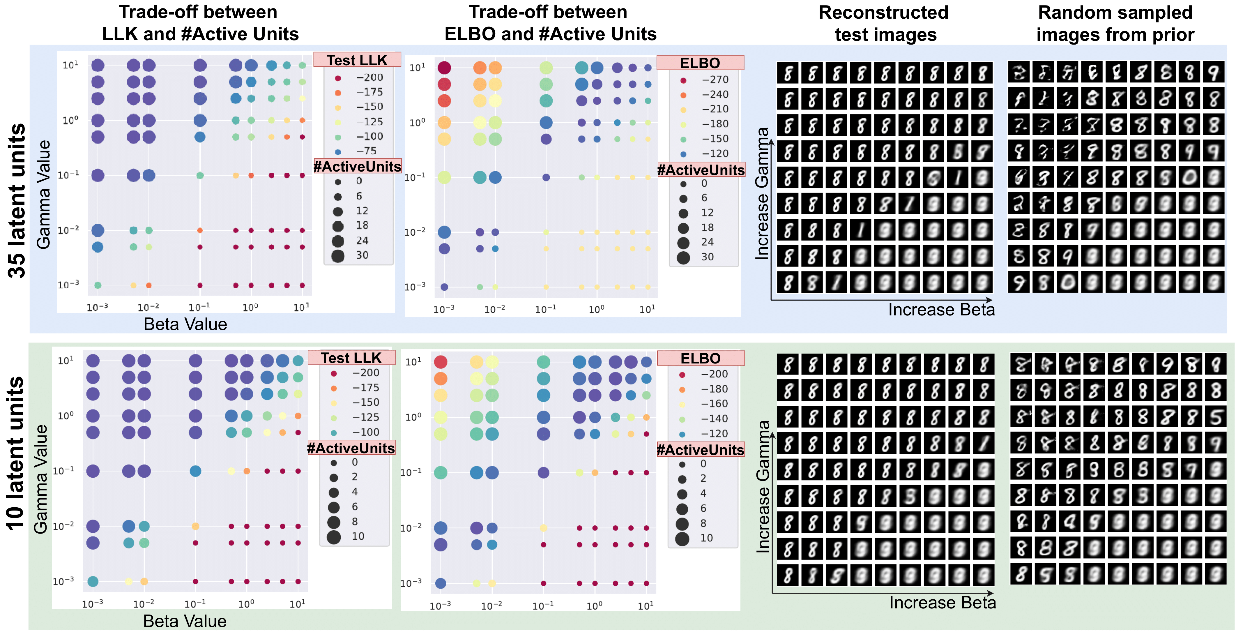
Figure 5: Another way to view the rate-distortion trade-off in VAE. Top row shows the trade-off for a VAE with 35 latent units while the bottom row is a VAE with 10 latent units. Test LLK is the log-likelihood on test set of a VAE with given (γ,β)𝛾𝛽(\gamma,\beta) values (higher value is desirable, thus the blue colored dots are better models). ELBO is the ELBO on test set (blue dots are higher values). #Active Units is the number of active latent units, i.e. the units don’t collapse to their prior. The position of the images is coordinated to the position of the dots, i.e. image and dot in the same row and column have the same (γ,β)𝛾𝛽(\gamma,\beta) values. Same network architectures and training configurations were used for all runs.

Hypothesis 1: The ELBO “game” must involve two players (encoder and decoder) play optimally (Section 2.2). Figure 5 shows that equal values for (γ,β)𝛾𝛽(\gamma,\beta) (the bottom left - top right diagonal line) give the best ELBO as well as the best quality of reconstructed test image and random sampled images. Increasing γ𝛾\gamma as in Bozkurt et al. has better log-likelihood but disappointing sampling quality, while increasing β𝛽\beta as in Higgins et al. [2017] causes the encoder to ignore all the image details and results the worst performance in all the benchmarks.

Hypothesis 2: It is hard to control the generation in VAEs with high capacity latents (Section 3). Increasing γ𝛾\gamma enables VAE to capture more image details which increase the latent capacity and the number of active latent units (Figure 5). In practice, this would be the simplest and most effective solution for the posterior collapse issue in VAE. While the random sampled images from high-γ𝛾\gamma VAE with 10 latent dimensions does resemble number “8” (Figure 5 bottom rightmost figure), VAE with 35 latent dimensions generates a mixed pattern of number “8”. However, the mixture of patterns includes more details (the line thickness, orientation, and ratio). Hence, we suspect that the extra activated units coupled with more details make it more difficult for the decoder to search through the meaningful combination of latent representation.
Refer to caption
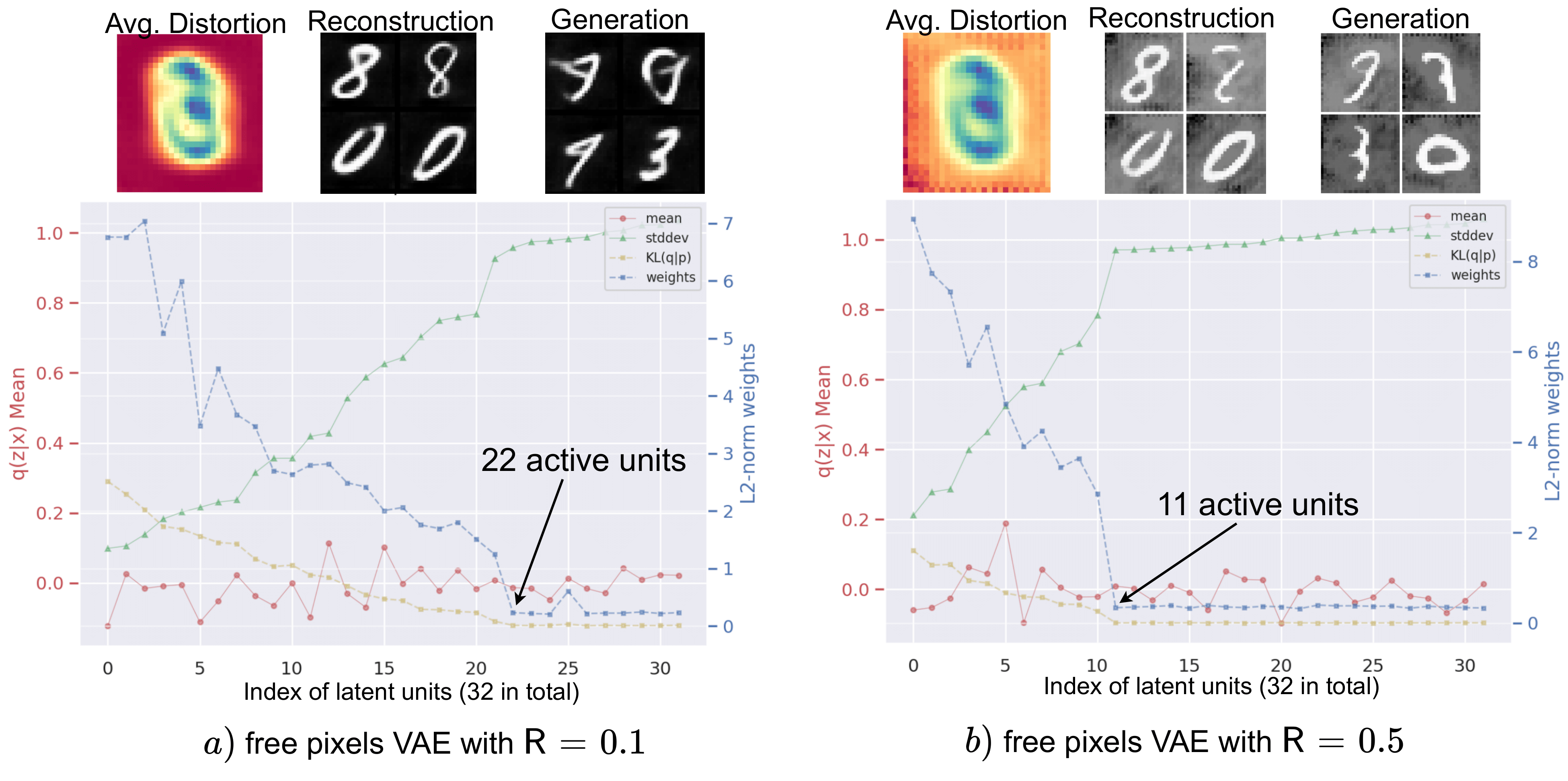
Figure 6: Statistics of latent units for VAEs with different values for the “free likelihood” constant 𝖱𝖱\mathsf{R}.

Hypothesis 3: MLE decoder doesn’t facilitate extrapolation (Section 2.3). Figure 6 shows that simply constrain the upper bound of likelihood won’t resolve the issue with the learning mechanism of MLE. The MLE learner doesn’t focus on the high detail (low density) region until all the high-density regions are optimized. This is due to the direction of maximum likelihood learning takes the form of D𝙺𝙻(p(𝐱)||q(𝐱))\mathrm{D}_{\mathtt{KL}}({p(\mathbf{x})}||{q(\mathbf{x})}) Bishop [2006], any area with high likelihood (the empty region in MNIST image) receives significant more weight than high information details that only occasionally appeared in the image.

Refer to caption
Figure 7: In a)a) and b)b), we vary the total number of latent units given the same network architectures, the networks trained on MNIST and CIFAR10 respectively. The dot size indicates how many latent units are active. Unet-VAE is a vanilla VAE with shortcut connection between every respectively encoder and decoder layers. c)c) show the same VAE trained with different β𝛽\beta value. The blue dots are the models trained for 200000 iterations. The orange dots are the models trained for 100000 iterations, then the encoder’s weights are fixed, and a new decoder is “plug-in” and trained for another 100000 iterations.

Hypothesis 4: VAE converges to the same number of active units regardless of the total number of latent units (Section 2.4). Figure 7-a shows that for the given network architectures the VAE could only utilize 7 latent units at maximum. Given less than 7 latent units, an implicit constraint is placed for the encoder that the image details are reduced (i.e. blurry image) even though all latent units are activated. In contrast, the VAE decoder ignores all redundant units if more than 7 latent units are given. This indicates that the given network architectures have an upper bound for how much information of observation it could learn and pass through the bottleneck. The same phenomenon applied for CIFAR10 dataset (Figure 7-b), however, we could clearly observe how much more details the VAE is capable of capturing given more latent units.

Hypothesis 5: The autoencoder design prevents fine detail information reaching the bottleneck (Section 2.4). To understand if the ELBO or the autoencoder design imposes an upper limit on the test log-likelihood of VAE, we propose Unet-VAE (Figure 7-b) which introduces shortcut connection between every encoder and decoder layer respectively. Ultimately, this causes the network to completely ignore the latent in the bottleneck. However, a significant amount of fine details including the texture of the frog skin are recovered in the reconstructed image. We suspect that the autoencoder design doesn’t allow low-level features (i.e. the fine details) learned from the lower layer to reach the bottleneck, thus the design of Hierarchical VAE tackles this issue and achieved great success in generating realistic images Kingma et al. [2016], Child [2021].

Hypothesis 6: The encoder imposes an upper bound to the mutual information of the decoder (Section 2.4). Figure 7-c shows the difference between a VAE with and without a fine-tuned decoder. In conclusion, fine-tuning the decoder doesn’t improve the log-likelihood on the test set or the reconstruction quality of the test image. Notably, the same observation is repeated for all VAE with different latent capacity, i.e. different β𝛽\beta values.

Let denote the information stored in the latents of a VAE is I(𝐱,𝐳)I𝐱𝐳\mathrm{I}(\mathbf{x},\mathbf{z}), the fine-tuned decoder learn to reconstruct image 𝐱^^𝐱\mathbf{\hat{x}} from the fixed latent 𝐳𝐳\mathbf{z}, then we have three variables form the Markov chain 𝐱𝐳𝐱^𝐱𝐳^𝐱\mathbf{x}\to\mathbf{z}\to\mathbf{\hat{x}}, and according to the data processing inequality Cover and Thomas [2006], I(𝐱,𝐳)I(𝐱^,𝐳)I𝐱𝐳I^𝐱𝐳\mathrm{I}(\mathbf{x},\mathbf{z})\geq\mathrm{I}(\mathbf{\hat{x}},\mathbf{z}). In other words, the pretrained encoder places an upper bound on the mutual information of the fine-tuned decoder, proof for the Proposition 2.

A total of 701 experiments on a single GTX 1080 GPU have been run for this section.

A.3 Proof of Theorem 2: Transitive Information

Proof.

The following properties of entropy is true for any given set of three random variables 𝐱𝐱\mathbf{x}, 𝐲𝐲\mathbf{y} and 𝐳𝐳\mathbf{z}:

  • I(𝐱,𝐳)=H(𝐱)H(𝐱|𝐳)I𝐱𝐳H𝐱Hconditional𝐱𝐳\mathrm{I}(\mathbf{x},\mathbf{z})=\mathrm{H}(\mathbf{x})-\mathrm{H}(\mathbf{x|z}), similar derivations for I(𝐱,𝐲)I𝐱𝐲\mathrm{I}(\mathbf{x},\mathbf{y}) and I(𝐲,𝐳)I𝐲𝐳\mathrm{I}(\mathbf{y},\mathbf{z})

  • H(𝐱,𝐲)=H(𝐱|𝐲)+H(𝐲)H𝐱𝐲Hconditional𝐱𝐲H𝐲\mathrm{H}(\mathbf{x,y})=\mathrm{H}(\mathbf{x|y})+\mathrm{H}(\mathbf{y}), and H(𝐱,𝐲|𝐳)=H(𝐱|𝐲,𝐳)+H(𝐲|𝐳)H𝐱conditional𝐲𝐳Hconditional𝐱𝐲𝐳Hconditional𝐲𝐳\mathrm{H}(\mathbf{x,y|z})=\mathrm{H}(\mathbf{x|y,z})+\mathrm{H}(\mathbf{y|z})

  • H(𝐱|𝐳)H(𝐱,𝐲|𝐳)Hconditional𝐱𝐳H𝐱conditional𝐲𝐳\mathrm{H}(\mathbf{x|z})\leq\mathrm{H}(\mathbf{x,y|z})

  • H(𝐱|𝐲,𝐳)H(𝐱|𝐲)Hconditional𝐱𝐲𝐳Hconditional𝐱𝐲\mathrm{H}(\mathbf{x|y,z})\leq\mathrm{H}(\mathbf{x|y})

We have:

H(𝐱|𝐳)Hconditional𝐱𝐳\displaystyle\mathrm{H}(\mathbf{x|z}) \displaystyle\leq H(𝐱,𝐲|𝐳)H𝐱conditional𝐲𝐳\displaystyle\quad\quad\mathrm{H}(\mathbf{x,y|z})
iff\displaystyle\iff H(𝐱|𝐳)Hconditional𝐱𝐳\displaystyle\mathrm{H}(\mathbf{x|z}) \displaystyle\leq H(𝐱|𝐲,𝐳)+H(𝐲|𝐳)Hconditional𝐱𝐲𝐳Hconditional𝐲𝐳\displaystyle\quad\quad\mathrm{H}(\mathbf{x|y,z})+\mathrm{H}(\mathbf{y|z})
iff\displaystyle\iff H(𝐱|𝐳)Hconditional𝐱𝐳\displaystyle\mathrm{H}(\mathbf{x|z}) \displaystyle\leq H(𝐱|𝐲)+H(𝐲|𝐳)Hconditional𝐱𝐲Hconditional𝐲𝐳\displaystyle\quad\quad\mathrm{H}(\mathbf{x|y})+\mathrm{H}(\mathbf{y|z})
iff\displaystyle\iff H(𝐱)H(𝐱|𝐳)H𝐱Hconditional𝐱𝐳\displaystyle\mathrm{H}(\mathbf{x})-\mathrm{H}(\mathbf{x|z}) \displaystyle\geq H(𝐱)H(𝐱|𝐲)+H(𝐲)H(𝐲|𝐳)H(𝐲)H𝐱Hconditional𝐱𝐲H𝐲Hconditional𝐲𝐳H𝐲\displaystyle\quad\quad\mathrm{H}(\mathbf{x})-\mathrm{H}(\mathbf{x|y})+\mathrm{H}(\mathbf{y})-\mathrm{H}(\mathbf{y|z})-\mathrm{H}(\mathbf{y})
iff\displaystyle\iff I(𝐱,𝐳)I𝐱𝐳\displaystyle\mathrm{I}(\mathbf{x},\mathbf{z}) \displaystyle\geq I(𝐱,𝐲)+I(𝐲,𝐳)H(𝐲)I𝐱𝐲I𝐲𝐳H𝐲\displaystyle\quad\quad\mathrm{I}(\mathbf{x},\mathbf{y})+\mathrm{I}(\mathbf{y},\mathbf{z})-\mathrm{H}(\mathbf{y})

As a result, Theorem 2 is proven. It is notable that the proof share the same approach as the variation of information metric in Meilă [2003].

A.4 ELBOs derivation for SemafoVAE

According to Figure 3-c, the modeling assumption of SemafoVAE are:

  • p(𝐱,𝐲,𝐳)=p(𝐱|𝐳)p(𝐳|𝐲)p(𝐲)𝑝𝐱𝐲𝐳𝑝conditional𝐱𝐳𝑝conditional𝐳𝐲𝑝𝐲p(\mathbf{x},\mathbf{y},\mathbf{z})=p(\mathbf{x}|\mathbf{z})p(\mathbf{z}|\mathbf{y})p(\mathbf{y}) for the generative model, and

  • q(𝐱,𝐲,𝐳)=q(𝐱)q(𝐳|𝐱)q(𝐲|𝐳)𝑞𝐱𝐲𝐳𝑞𝐱𝑞conditional𝐳𝐱𝑞conditional𝐲𝐳q(\mathbf{x},\mathbf{y},\mathbf{z})=q(\mathbf{x})q(\mathbf{z}|\mathbf{x})q(\mathbf{y}|\mathbf{z}) for the inference model (the parameters are omitted in all derivations within this section).

ELBO derivation for unsupervised learning

logp(𝐱)𝑝𝐱\displaystyle\log p(\mathbf{x}) =logz,yp(𝐱,𝐲,𝐳)dzdyabsentsubscript𝑧𝑦𝑝𝐱𝐲𝐳differential-d𝑧differential-d𝑦\displaystyle=\log\int_{z,y}p(\mathbf{x},\mathbf{y},\mathbf{z})\mathrm{d}z\mathrm{d}y
=logzp(𝐱,𝐲,𝐳)q(𝐳,𝐲|𝐱)q(𝐳,𝐲|𝐱)dzabsentsubscript𝑧𝑝𝐱𝐲𝐳𝑞𝐳conditional𝐲𝐱𝑞𝐳conditional𝐲𝐱differential-d𝑧\displaystyle=\log\int_{z}\frac{p(\mathbf{x},\mathbf{y},\mathbf{z})}{q(\mathbf{z},\mathbf{y}|\mathbf{x})}q(\mathbf{z},\mathbf{y}|\mathbf{x})\mathrm{d}z
=logEq(𝐳,𝐲|𝐱)[p(𝐱|𝐳)p(𝐳|𝐲)p(𝐲)q(𝐳|𝐱)q(𝐲|𝐳)]absentsubscriptE𝑞𝐳conditional𝐲𝐱delimited-[]𝑝conditional𝐱𝐳𝑝conditional𝐳𝐲𝑝𝐲𝑞conditional𝐳𝐱𝑞conditional𝐲𝐳\displaystyle=\log\mathrm{E}_{q(\mathbf{z},\mathbf{y}|\mathbf{x})}\bigg{[}\frac{p(\mathbf{x}|\mathbf{z})p(\mathbf{z}|\mathbf{y})p(\mathbf{y})}{q(\mathbf{z}|\mathbf{x})q(\mathbf{y}|\mathbf{z})}\bigg{]}

Applying Jensen’s inequality:

logp(𝐱)log𝑝𝐱\displaystyle\mathrm{log}p(\mathbf{x}) Eq(𝐳|𝐱)q(𝐲|𝐳)[logp(𝐱|𝐳)p(𝐳|𝐲)p(𝐲)q(𝐳|𝐱)q(𝐲|𝐳)]absentsubscriptE𝑞conditional𝐳𝐱𝑞conditional𝐲𝐳delimited-[]log𝑝conditional𝐱𝐳𝑝conditional𝐳𝐲𝑝𝐲𝑞conditional𝐳𝐱𝑞conditional𝐲𝐳\displaystyle\geq\mathrm{E}_{q(\mathbf{z}|\mathbf{x})q(\mathbf{y}|\mathbf{z})}\bigg{[}\mathrm{log}\frac{p(\mathbf{x}|\mathbf{z})p(\mathbf{z}|\mathbf{y})p(\mathbf{y})}{q(\mathbf{z}|\mathbf{x})q(\mathbf{y}|\mathbf{z})}\bigg{]} (16)
=Eq(𝐳|𝐱)[logp(𝐱|𝐳)]Eq(𝐳|𝐱)q(𝐲|𝐳)[logq(𝐳|𝐱)p(𝐳|𝐲)]Eq(𝐳|𝐱)q(𝐲|𝐳)[logq(𝐲|𝐳)p(𝐲)]absentsubscriptE𝑞conditional𝐳𝐱delimited-[]log𝑝conditional𝐱𝐳subscriptE𝑞conditional𝐳𝐱𝑞conditional𝐲𝐳delimited-[]log𝑞conditional𝐳𝐱𝑝conditional𝐳𝐲subscriptE𝑞conditional𝐳𝐱𝑞conditional𝐲𝐳delimited-[]log𝑞conditional𝐲𝐳𝑝𝐲\displaystyle=\mathrm{E}_{q(\mathbf{z}|\mathbf{x})}\big{[}\mathrm{log}p(\mathbf{x}|\mathbf{z})\big{]}-\mathrm{E}_{q(\mathbf{z}|\mathbf{x})q(\mathbf{y}|\mathbf{z})}\bigg{[}\mathrm{log}\frac{q(\mathbf{z}|\mathbf{x})}{p(\mathbf{z}|\mathbf{y})}\bigg{]}-\mathrm{E}_{q(\mathbf{z}|\mathbf{x})q(\mathbf{y}|\mathbf{z})}\bigg{[}\mathrm{log}\frac{q(\mathbf{y}|\mathbf{z})}{p(\mathbf{y})}\bigg{]}
=Eq(𝐳|𝐱)[logp(𝐱|𝐳)]Eq(𝐲|𝐳)[D𝙺𝙻(q(𝐳|𝐱)||p(𝐳|𝐲))]Eq(𝐳|𝐱)[D𝙺𝙻(q(𝐲|𝐳)||p(𝐲))]\displaystyle=\mathrm{E}_{q(\mathbf{z}|\mathbf{x})}\big{[}\mathrm{log}p(\mathbf{x}|\mathbf{z})\big{]}-\mathrm{E}_{q(\mathbf{y}|\mathbf{z})}\big{[}\mathrm{D}_{\mathtt{KL}}({q(\mathbf{z}|\mathbf{x})}||{p(\mathbf{z}|\mathbf{y})})\big{]}-\mathrm{E}_{q(\mathbf{z}|\mathbf{x})}\big{[}\mathrm{D}_{\mathtt{KL}}({q(\mathbf{y}|\mathbf{z})}||{p(\mathbf{y})})\big{]}
=𝚄(𝐱,𝐳)absentsubscript𝚄𝐱𝐳\displaystyle=\mathcal{E}_{\mathtt{U}}(\mathbf{x},\mathbf{z})

ELBO derivation for supervised learning:

logp(𝐱,𝐲)𝑝𝐱𝐲\displaystyle\log p(\mathbf{x},\mathbf{y}) =logzp(𝐱,𝐲,𝐳)dzabsentlogsubscript𝑧𝑝𝐱𝐲𝐳differential-d𝑧\displaystyle=\mathrm{log}\int_{z}p(\mathbf{x},\mathbf{y},\mathbf{z})\mathrm{d}z (17)
=logEq(𝐳|𝐱)[p(𝐱|𝐳)p(𝐳|𝐲)p(𝐲)q(𝐳|𝐱)]absentsubscriptlogE𝑞conditional𝐳𝐱delimited-[]𝑝conditional𝐱𝐳𝑝conditional𝐳𝐲𝑝𝐲𝑞conditional𝐳𝐱\displaystyle=\mathrm{log}\mathrm{E}_{q(\mathbf{z}|\mathbf{x})}\bigg{[}\frac{p(\mathbf{x}|\mathbf{z})p(\mathbf{z}|\mathbf{y})p(\mathbf{y})}{q(\mathbf{z}|\mathbf{x})}\bigg{]}
Eq(𝐳|𝐱)[logp(𝐱|𝐳)p(𝐳|𝐲)p(𝐲)q(𝐳|𝐱)]absentsubscriptE𝑞conditional𝐳𝐱delimited-[]log𝑝conditional𝐱𝐳𝑝conditional𝐳𝐲𝑝𝐲𝑞conditional𝐳𝐱\displaystyle\geq\mathrm{E}_{q(\mathbf{z}|\mathbf{x})}\bigg{[}\mathrm{log}\frac{p(\mathbf{x}|\mathbf{z})p(\mathbf{z}|\mathbf{y})p(\mathbf{y})}{q(\mathbf{z}|\mathbf{x})}\bigg{]}
=Eq(𝐳|𝐱)[logp(𝐱|𝐳)]D𝙺𝙻(q(𝐳|𝐱)||p(𝐳|𝐲))+logp(𝐲)\displaystyle=\mathrm{E}_{q(\mathbf{z}|\mathbf{x})}\big{[}\mathrm{log}p(\mathbf{x}|\mathbf{z})\big{]}-\mathrm{D}_{\mathtt{KL}}({q(\mathbf{z}|\mathbf{x})}||{p(\mathbf{z}|\mathbf{y})})+\mathrm{log}p(\mathbf{y})
=𝚂(𝐱,𝐲,𝐳)absentsubscript𝚂𝐱𝐲𝐳\displaystyle=\mathcal{E}_{\mathtt{S}}(\mathbf{x},\mathbf{y},\mathbf{z})

We introduce the latent variables 𝐮𝐮\mathbf{u} to maximize the ELBO of logp(𝐲)𝑝𝐲\log p(\mathbf{y}):

logp(𝐲)Eq(𝐮|𝐲)[logp(𝐲|𝐮)]D𝙺𝙻(q(𝐮|𝐲)||p(𝐮))=(𝐲,𝐮)\displaystyle\mathrm{log}p(\mathbf{y})\geq\mathrm{E}_{q(\mathbf{u}|\mathbf{y})}\big{[}\log p(\mathbf{y}|\mathbf{u})\big{]}-\mathrm{D}_{\mathtt{KL}}({q(\mathbf{u}|\mathbf{y})}||{p(\mathbf{u})})=\mathcal{E}(\mathbf{y},\mathbf{u}) (18)

We derive the upper bound for D𝙺𝙻(q(𝐳|𝐱)||p(𝐳||𝐲))\mathrm{D}_{\mathtt{KL}}({q(\mathbf{z}|\mathbf{x})}||{p(\mathbf{z}||\mathbf{y})}), assumed the factorization p(𝐳,𝐲,𝐮)=p(𝐲|𝐮)p(𝐳|𝐮)p(𝐮)𝑝𝐳𝐲𝐮𝑝conditional𝐲𝐮𝑝conditional𝐳𝐮𝑝𝐮p(\mathbf{z},\mathbf{y},\mathbf{u})=p(\mathbf{y}|\mathbf{u})p(\mathbf{z}|\mathbf{u})p(\mathbf{u}).

D𝙺𝙻(q(𝐳|𝐱)||p(𝐳||𝐲))\displaystyle\mathrm{D}_{\mathtt{KL}}({q(\mathbf{z}|\mathbf{x})}||{p(\mathbf{z}||\mathbf{y})}) (19)
=\displaystyle= Eq(𝐳|𝐱)[logq(𝐳|𝐱)p(𝐳|𝐲)]subscriptE𝑞conditional𝐳𝐱delimited-[]log𝑞conditional𝐳𝐱𝑝conditional𝐳𝐲\displaystyle\mathrm{E}_{q(\mathbf{z}|\mathbf{x})}\bigg{[}\mathrm{log}\frac{q(\mathbf{z}|\mathbf{x})}{p(\mathbf{z}|\mathbf{y})}\bigg{]}
=\displaystyle= Eq(𝐳|𝐱)[logq(𝐳|𝐱)]Eq(𝐳|𝐱)[logp(𝐳|𝐲)]subscriptE𝑞conditional𝐳𝐱delimited-[]log𝑞conditional𝐳𝐱subscriptE𝑞conditional𝐳𝐱delimited-[]log𝑝conditional𝐳𝐲\displaystyle\mathrm{E}_{q(\mathbf{z}|\mathbf{x})}\big{[}\mathrm{log}q(\mathbf{z}|\mathbf{x})\big{]}-\mathrm{E}_{q(\mathbf{z}|\mathbf{x})}\big{[}\mathrm{log}p(\mathbf{z}|\mathbf{y})\big{]}
=\displaystyle= Eq(𝐳|𝐱)[logq(𝐳|𝐱)]Eq(𝐳|𝐱)[logp(𝐳,𝐲)]+Eq(𝐳|𝐱)[logp(𝐲)]subscriptE𝑞conditional𝐳𝐱delimited-[]log𝑞conditional𝐳𝐱subscriptE𝑞conditional𝐳𝐱delimited-[]log𝑝𝐳𝐲subscriptE𝑞conditional𝐳𝐱delimited-[]log𝑝𝐲\displaystyle\mathrm{E}_{q(\mathbf{z}|\mathbf{x})}\big{[}\mathrm{log}q(\mathbf{z}|\mathbf{x})\big{]}-\mathrm{E}_{q(\mathbf{z}|\mathbf{x})}\big{[}\mathrm{log}p(\mathbf{z},\mathbf{y})\big{]}+\mathrm{E}_{q(\mathbf{z}|\mathbf{x})}\big{[}\mathrm{log}p(\mathbf{y})\big{]}
=\displaystyle= Eq(𝐳|𝐱)[logq(𝐳|𝐱)]Eq(𝐳|𝐱)[logup(𝐳,𝐲,𝐮)du]+Eq(𝐳|𝐱)[logp(𝐲)]subscriptE𝑞conditional𝐳𝐱delimited-[]log𝑞conditional𝐳𝐱subscriptE𝑞conditional𝐳𝐱delimited-[]logsubscript𝑢𝑝𝐳𝐲𝐮differential-d𝑢subscriptE𝑞conditional𝐳𝐱delimited-[]log𝑝𝐲\displaystyle\mathrm{E}_{q(\mathbf{z}|\mathbf{x})}\big{[}\mathrm{log}q(\mathbf{z}|\mathbf{x})\big{]}-\mathrm{E}_{q(\mathbf{z}|\mathbf{x})}\big{[}\mathrm{log}\int_{u}p(\mathbf{z},\mathbf{y},\mathbf{u})\mathrm{d}u\big{]}+\mathrm{E}_{q(\mathbf{z}|\mathbf{x})}\big{[}\mathrm{log}p(\mathbf{y})\big{]}
=\displaystyle= Eq(𝐳|𝐱)[logq(𝐳|𝐱)]Eq(𝐳|𝐱)[logup(𝐳,𝐲,𝐮)q(𝐮|𝐲)q(𝐮|𝐲)du]Eq(𝐳|𝐱)q(𝐮|𝐲)[logp(𝐳,𝐲,𝐮)q(𝐮|𝐲)](Jensen inequality)+Eq(𝐳|𝐱)[logp(𝐲)]subscriptE𝑞conditional𝐳𝐱delimited-[]log𝑞conditional𝐳𝐱subscriptsubscriptE𝑞conditional𝐳𝐱delimited-[]logsubscript𝑢𝑝𝐳𝐲𝐮𝑞conditional𝐮𝐲𝑞conditional𝐮𝐲differential-d𝑢absentsubscriptE𝑞conditional𝐳𝐱𝑞conditional𝐮𝐲delimited-[]log𝑝𝐳𝐲𝐮𝑞conditional𝐮𝐲(Jensen inequality)subscriptE𝑞conditional𝐳𝐱delimited-[]log𝑝𝐲\displaystyle\mathrm{E}_{q(\mathbf{z}|\mathbf{x})}\big{[}\mathrm{log}q(\mathbf{z}|\mathbf{x})\big{]}-\underbrace{\mathrm{E}_{q(\mathbf{z}|\mathbf{x})}\big{[}\mathrm{log}\int_{u}\frac{p(\mathbf{z},\mathbf{y},\mathbf{u})q(\mathbf{u}|\mathbf{y})}{q(\mathbf{u}|\mathbf{y})}\mathrm{d}u\big{]}}_{\geq\mathrm{E}_{q(\mathbf{z}|\mathbf{x})q(\mathbf{u}|\mathbf{y})}\big{[}\mathrm{log}\frac{p(\mathbf{z},\mathbf{y},\mathbf{u})}{q(\mathbf{u}|\mathbf{y})}\big{]}\text{(Jensen inequality)}}+\mathrm{E}_{q(\mathbf{z}|\mathbf{x})}\big{[}\mathrm{log}p(\mathbf{y})\big{]}
\displaystyle\leq Eq(𝐳|𝐱)[logq(𝐳|𝐱)]Eq(𝐳|𝐱)q(𝐮|𝐲)[logp(𝐲|𝐮)p(𝐳|𝐮)p(𝐮)q(𝐮|𝐲)]+Eq(𝐳|𝐱)[logp(𝐲)]subscriptE𝑞conditional𝐳𝐱delimited-[]log𝑞conditional𝐳𝐱subscriptE𝑞conditional𝐳𝐱𝑞conditional𝐮𝐲delimited-[]log𝑝conditional𝐲𝐮𝑝conditional𝐳𝐮𝑝𝐮𝑞conditional𝐮𝐲subscriptE𝑞conditional𝐳𝐱delimited-[]log𝑝𝐲\displaystyle\mathrm{E}_{q(\mathbf{z}|\mathbf{x})}\big{[}\mathrm{log}q(\mathbf{z}|\mathbf{x})\big{]}-\mathrm{E}_{q(\mathbf{z}|\mathbf{x})q(\mathbf{u}|\mathbf{y})}\bigg{[}\mathrm{log}\frac{p(\mathbf{y}|\mathbf{u})p(\mathbf{z}|\mathbf{u})p(\mathbf{u})}{q(\mathbf{u}|\mathbf{y})}\bigg{]}+\mathrm{E}_{q(\mathbf{z}|\mathbf{x})}\big{[}\mathrm{log}p(\mathbf{y})\big{]}
=\displaystyle= Eq(𝐳|𝐱)q(𝐮|𝐲)[D𝙺𝙻(q(𝐳|𝐱)||p(𝐳|𝐮))](𝐲,𝐮)+logp(𝐲)\displaystyle\mathrm{E}_{q(\mathbf{z}|\mathbf{x})q(\mathbf{u}|\mathbf{y})}\big{[}\mathrm{D}_{\mathtt{KL}}({q(\mathbf{z}|\mathbf{x})}||{p(\mathbf{z}|\mathbf{u})})\big{]}-\mathcal{E}(\mathbf{y},\mathbf{u})+\log p(\mathbf{y})

where (𝐲,𝐮)𝐲𝐮\mathcal{E}(\mathbf{y},\mathbf{u}) is defined by (18). Finally, we substitute (19) to (16) and (17) which eliminates the need for maximizing the intractable evidence logp(𝐲)log𝑝𝐲\mathrm{log}p(\mathbf{y}) and replace 𝐲𝐲\mathbf{y} by the tractable latents 𝐮𝐮\mathbf{u} in all of our KL divergence terms.

The final unsupervised and supervised ELBO for SemafoVAE are:

𝚄(𝐱,𝐳)subscript𝚄𝐱𝐳\displaystyle\mathcal{E}_{\mathtt{U}}(\mathbf{x},\mathbf{z}) =Eq(𝐳|𝐱)[logp(𝐱|𝐳)]Eq(𝐲|𝐳)[D𝙺𝙻(q(𝐳|𝐱||p(𝐳|𝐲))]Eq(𝐳|𝐱)[D𝙺𝙻(q(𝐲|𝐳)||p(𝐲))]\displaystyle=\mathrm{E}_{q(\mathbf{z}|\mathbf{x})}\big{[}\mathrm{log}p(\mathbf{x}|\mathbf{z})\big{]}-\mathrm{E}_{q(\mathbf{y}|\mathbf{z})}\big{[}\mathrm{D}_{\mathtt{KL}}({q(\mathbf{z}|\mathbf{x}}||{p(\mathbf{z}|\mathbf{y})})\big{]}-\mathrm{E}_{q(\mathbf{z}|\mathbf{x})}\big{[}\mathrm{D}_{\mathtt{KL}}({q(\mathbf{y}|\mathbf{z})}||{p(\mathbf{y})})\big{]} (20)
Eq(𝐳|𝐱)[logp(𝐱|𝐳)]absentlimit-fromsubscriptE𝑞conditional𝐳𝐱delimited-[]log𝑝conditional𝐱𝐳\displaystyle\geq\mathrm{E}_{q(\mathbf{z}|\mathbf{x})}\big{[}\mathrm{log}p(\mathbf{x}|\mathbf{z})\big{]}-
Eq(𝐲|𝐳)[Eq(𝐳|𝐱)q(𝐮|𝐲)[D𝙺𝙻(q(𝐳|𝐱)||p(q(𝐳|𝐮))]+(𝐲,𝐮)logp(𝐲)]\displaystyle\quad\quad\mathrm{E}_{q(\mathbf{y}|\mathbf{z})}\bigg{[}\mathrm{E}_{q(\mathbf{z}|\mathbf{x})q(\mathbf{u}|\mathbf{y})}\big{[}\mathrm{D}_{\mathtt{KL}}({q(\mathbf{z}|\mathbf{x})}||{p(q(\mathbf{z}|\mathbf{u})})\big{]}+\mathcal{E}(\mathbf{y},\mathbf{u})-\log p(\mathbf{y})\bigg{]}-
(Eq(𝐳|𝐱)[logq(𝐲|𝐳)]Eq(𝐲|𝐳)[logp(𝐲)])subscriptE𝑞conditional𝐳𝐱delimited-[]log𝑞conditional𝐲𝐳subscriptE𝑞conditional𝐲𝐳delimited-[]log𝑝𝐲\displaystyle\quad\quad\bigg{(}\mathrm{E}_{q(\mathbf{z}|\mathbf{x})}\big{[}\mathrm{log}q(\mathbf{y}|\mathbf{z})\big{]}-\mathrm{E}_{q(\mathbf{y}|\mathbf{z})}\big{[}\mathrm{log}p(\mathbf{y})\big{]}\bigg{)}
=Eq(𝐳|𝐱)[logp(𝐱|𝐳)]Eq(𝐳,𝐲,𝐮|𝐱)[D𝙺𝙻(q(𝐳|𝐱)||p(𝐳|𝐮))]+Eq(𝐲|𝐳)[(𝐲,𝐮)]\displaystyle=\mathrm{E}_{q(\mathbf{z}|\mathbf{x})}\big{[}\mathrm{log}p(\mathbf{x}|\mathbf{z})\big{]}-\mathrm{E}_{q(\mathbf{z},\mathbf{y},\mathbf{u}|\mathbf{x})}\big{[}\mathrm{D}_{\mathtt{KL}}({q(\mathbf{z}|\mathbf{x})}||{p(\mathbf{z}|\mathbf{u})})\big{]}+\mathrm{E}_{q(\mathbf{y}|\mathbf{z})}\big{[}\mathcal{E}(\mathbf{y},\mathbf{u})\big{]}-
Eq(𝐳|𝐱)[logq(𝐲|𝐳)]subscriptE𝑞conditional𝐳𝐱delimited-[]log𝑞conditional𝐲𝐳\displaystyle\quad\quad\mathrm{E}_{q(\mathbf{z}|\mathbf{x})}\big{[}\mathrm{log}q(\mathbf{y}|\mathbf{z})\big{]}

and

𝚂(𝐱,𝐲,𝐳)subscript𝚂𝐱𝐲𝐳\displaystyle\mathcal{E}_{\mathtt{S}}(\mathbf{x},\mathbf{y},\mathbf{z}) =Eq(𝐳|𝐱)[logp(𝐱|𝐳)]D𝙺𝙻(q(𝐳|𝐱)||p(𝐳|𝐲))+logp(𝐲)\displaystyle=\mathrm{E}_{q(\mathbf{z}|\mathbf{x})}\big{[}\mathrm{log}p(\mathbf{x}|\mathbf{z})\big{]}-\mathrm{D}_{\mathtt{KL}}({q(\mathbf{z}|\mathbf{x})}||{p(\mathbf{z}|\mathbf{y})})+\mathrm{log}p(\mathbf{y}) (21)
Eq(𝐳|𝐱)[logp(𝐱|𝐳)]absentlimit-fromsubscriptE𝑞conditional𝐳𝐱delimited-[]𝑝conditional𝐱𝐳\displaystyle\geq\mathrm{E}_{q(\mathbf{z}|\mathbf{x})}\big{[}\log p(\mathbf{x}|\mathbf{z})\big{]}-
(Eq(𝐳|𝐱)q(𝐮|𝐲)[D𝙺𝙻(q(𝐳|𝐱)||p(𝐳|𝐮))](𝐲,𝐮)+logp(𝐲))+\displaystyle\quad\quad\bigg{(}\mathrm{E}_{q(\mathbf{z}|\mathbf{x})q(\mathbf{u}|\mathbf{y})}\big{[}\mathrm{D}_{\mathtt{KL}}({q(\mathbf{z}|\mathbf{x})}||{p(\mathbf{z}|\mathbf{u})})\big{]}-\mathcal{E}(\mathbf{y},\mathbf{u})+\log p(\mathbf{y})\bigg{)}+
logp(𝐲)𝑝𝐲\displaystyle\quad\quad\log p(\mathbf{y})
=Eq(𝐳|𝐱)[logp(𝐱|𝐳)]Eq(𝐳,𝐮|𝐱,𝐲)[D𝙺𝙻(q(𝐳|𝐱)||p(q(𝐳|𝐮))]+(𝐲,𝐮)fragmentsE𝑞conditional𝐳𝐱[p(x|z)]E𝑞𝐳conditional𝐮𝐱𝐲[D𝙺𝙻(q(z|x)||p(q(z|u))]E(y,u)\displaystyle=\mathrm{E}_{q(\mathbf{z}|\mathbf{x})}\big{[}\log p(\mathbf{x}|\mathbf{z})\big{]}-\mathrm{E}_{q(\mathbf{z},\mathbf{u}|\mathbf{x},\mathbf{y})}\big{[}\mathrm{D}_{\mathtt{KL}}({q(\mathbf{z}|\mathbf{x})}||{p(q(\mathbf{z}|\mathbf{u})})\big{]}+\mathcal{E}(\mathbf{y},\mathbf{u})

A.5 Hierarchical VAE and the Semafo prior
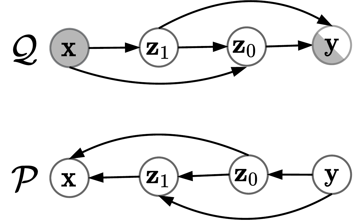
Refer to caption
Figure 8: Graphical model of Semafo Hierarchical VAE with two layers of hierarchical latent variables.

In the paper, we also apply the Semafo prior to Hierarchical VAE Kingma et al. [2016], Child [2021]. According to Figure 8, a system of L𝐿L-layers hierarchical variables assumes the factorization:

  • p(𝐱,𝐳,𝐲)=p(𝐱|𝐳0,,𝐳L)iLp(𝐳i|𝐳<i,𝐲)p(𝐲)fragmentsp(x,z,y)p(x|z0,,z𝐿)product𝑖𝐿p(z𝑖|zfragmentsi,y)p(y)p(\mathbf{x},\mathbf{z},\mathbf{y})=p(\mathbf{x}|\mathbf{z}_{0},...,\mathbf{z}_{L})\>\prod_{i}^{L}p(\mathbf{z}_{i}|\mathbf{z}_{<i},\mathbf{y})\>p(\mathbf{y}) and

  • q(𝐱,𝐳,𝐲)=q(𝐲|𝐳0,,𝐳L)iLq(𝐳i|𝐳<i,𝐱)q(𝐱)fragmentsq(x,z,y)q(y|z0,,z𝐿)product𝑖𝐿q(z𝑖|zfragmentsi,x)q(x)q(\mathbf{x},\mathbf{z},\mathbf{y})=q(\mathbf{y}|\mathbf{z}_{0},...,\mathbf{z}_{L})\>\prod_{i}^{L}q(\mathbf{z}_{i}|\mathbf{z}_{<i},\mathbf{x})\>q(\mathbf{x})

Since we only use two layers of the hierarchical latent variables 𝐳0fragmentsz0\mathbf{z}_{0} and 𝐳1fragmentsz1\mathbf{z}_{1}, the following derivation is only for such model, however, the same derivation could be generalized to more latent layers.

The unsupervised and supervised ELBO of SemafoHVAE are

𝚄(𝐱,𝐳)=fragmentsE𝚄(x,z)\displaystyle\mathcal{E}_{\mathtt{U}}(\mathbf{x},\mathbf{z})= Eq(𝐳|𝐱)[logp(𝐱|𝐳)]fragmentsEfragmentsq(z|x)[logp(x|z)]\displaystyle\;\mathrm{E}_{q(\mathbf{z}|\mathbf{x})}\big{[}\mathrm{log}p(\mathbf{x}|\mathbf{z})\big{]}-
Eq(𝐳0|𝐳1,𝐱)q(𝐲|𝐳0,𝐳1,𝐱)[D𝙺𝙻(q(𝐳1|𝐱)||p(𝐳1|𝐳0,𝐲))]fragmentsEfragmentsq(z0|z1,x)q(y|z0,z1,x)[D𝙺𝙻(q(z1|x)||p(z1|z0,y))]\displaystyle\;\mathrm{E}_{q(\mathbf{z}_{0}|\mathbf{z}_{1},\mathbf{x})q(\mathbf{y}|\mathbf{z}_{0},\mathbf{z}_{1},\mathbf{x})}\big{[}\mathrm{D}_{\mathtt{KL}}({q(\mathbf{z}_{1}|\mathbf{x})}||{p(\mathbf{z}_{1}|\mathbf{z}_{0},\mathbf{y})})\big{]}-
Eq(𝐳1|𝐱)q(𝐲|𝐳0,𝐳1,𝐱)[D𝙺𝙻(q(𝐳0|𝐳1,𝐱)||p(𝐳0|𝐲))]fragmentsEfragmentsq(z1|x)q(y|z0,z1,x)[D𝙺𝙻(q(z0|z1,x)||p(z0|y))]\displaystyle\;\mathrm{E}_{q(\mathbf{z}_{1}|\mathbf{x})q(\mathbf{y}|\mathbf{z}_{0},\mathbf{z}_{1},\mathbf{x})}\big{[}\mathrm{D}_{\mathtt{KL}}({q(\mathbf{z}_{0}|\mathbf{z}_{1},\mathbf{x})}||{p(\mathbf{z}_{0}|\mathbf{y})})\big{]}-
Eq(𝐳1|𝐱)q(𝐳0|𝐳1,𝐱)[D𝙺𝙻(q(𝐲|𝐳1,𝐳0,𝐱)||p(𝐲))]fragmentsEfragmentsq(z1|x)q(z0|z1,x)[D𝙺𝙻(q(y|z1,z0,x)||p(y))]\displaystyle\;\mathrm{E}_{q(\mathbf{z}_{1}|\mathbf{x})q(\mathbf{z}_{0}|\mathbf{z}_{1},\mathbf{x})}\big{[}\mathrm{D}_{\mathtt{KL}}({q(\mathbf{y}|\mathbf{z}_{1},\mathbf{z}_{0},\mathbf{x})}||{p(\mathbf{y})})\big{]} (22)
and
𝚄(𝐱,𝐲,𝐳)=fragmentsE𝚄(x,y,z)\displaystyle\mathcal{E}_{\mathtt{U}}(\mathbf{x},\mathbf{y},\mathbf{z})= Eq(𝐳|𝐱)[logp(𝐱|𝐳)]fragmentsEfragmentsq(z|x)[logp(x|z)]\displaystyle\;\mathrm{E}_{q(\mathbf{z}|\mathbf{x})}\big{[}\mathrm{log}p(\mathbf{x}|\mathbf{z})\big{]}-
Eq(𝐳0|𝐳1,𝐱)[D𝙺𝙻(q(𝐳1|𝐱)||p(𝐳1|𝐳0,𝐲))]fragmentsEfragmentsq(z0|z1,x)[D𝙺𝙻(q(z1|x)||p(z1|z0,y))]\displaystyle\;\mathrm{E}_{q(\mathbf{z}_{0}|\mathbf{z}_{1},\mathbf{x})}\big{[}\mathrm{D}_{\mathtt{KL}}({q(\mathbf{z}_{1}|\mathbf{x})}||{p(\mathbf{z}_{1}|\mathbf{z}_{0},\mathbf{y})})\big{]}-
Eq(𝐳1|𝐱)[D𝙺𝙻(q(𝐳0|𝐳1,𝐱)||p(𝐳0|𝐲))]+fragmentsEfragmentsq(z1|x)[D𝙺𝙻(q(z0|z1,x)||p(z0|y))]\displaystyle\;\mathrm{E}_{q(\mathbf{z}_{1}|\mathbf{x})}\big{[}\mathrm{D}_{\mathtt{KL}}({q(\mathbf{z}_{0}|\mathbf{z}_{1},\mathbf{x})}||{p(\mathbf{z}_{0}|\mathbf{y})})\big{]}+
logp(𝐲)fragmentslogp(y)\displaystyle\;\mathrm{log}p(\mathbf{y}) (23)

We expand the KL-terms for 𝐳0fragmentsz0\mathbf{z}_{0} and 𝐳1fragmentsz1\mathbf{z}_{1}

D𝙺𝙻(q(𝐳0|𝐳1,𝐱)||p(𝐳0|𝐲))fragmentsD𝙺𝙻(q(z0|z1,x)||p(z0|y))\displaystyle\mathrm{D}_{\mathtt{KL}}({q(\mathbf{z}_{0}|\mathbf{z}_{1},\mathbf{x})}||{p(\mathbf{z}_{0}|\mathbf{y})}) =Hq(𝐳𝟎|𝐳𝟏,𝐱)Eq(𝐳0|𝐳1,𝐱)[logp(𝐳0,𝐲)p(𝐲)]fragmentsHq(z0|z1,x)Efragmentsq(z0|z1,x)[logfragmentsp(z0,y)fragmentsp(y)]\displaystyle=-\mathrm{H}_{\mathrm{q}}(\mathbf{\mathbf{z}_{0}|\mathbf{z}_{1},\mathbf{x}})-\mathrm{E}_{q(\mathbf{z}_{0}|\mathbf{z}_{1},\mathbf{x})}\bigg{[}\mathrm{log}\frac{p(\mathbf{z}_{0},\mathbf{y})}{p(\mathbf{y})}\bigg{]} (24)
D𝙺𝙻(q(𝐳1|𝐱)||p(𝐳1|𝐳0,𝐲))fragmentsD𝙺𝙻(q(z1|x)||p(z1|z0,y))\displaystyle\mathrm{D}_{\mathtt{KL}}({q(\mathbf{z}_{1}|\mathbf{x})}||{p(\mathbf{z}_{1}|\mathbf{z}_{0},\mathbf{y})}) =Hq(𝐳𝟏|𝐱)Eq(𝐳1|𝐱)[logp(𝐳0,𝐳1,𝐲)p(𝐳0,𝐲)]fragmentsHq(z1|x)Efragmentsq(z1|x)[logfragmentsp(z0,z1,y)fragmentsp(z0,y)]\displaystyle=-\mathrm{H}_{\mathrm{q}}(\mathbf{\mathbf{z}_{1}|\mathbf{x}})-\mathrm{E}_{q(\mathbf{z}_{1}|\mathbf{x})}\bigg{[}\mathrm{log}\frac{p(\mathbf{z}_{0},\mathbf{z}_{1},\mathbf{y})}{p(\mathbf{z}_{0},\mathbf{y})}\bigg{]} (25)

Because logp(𝐳0,𝐲)fragmentslogp(z0,y)\mathrm{log}p(\mathbf{z}_{0},\mathbf{y}) is eliminated when summing (24) and (25), we focus on the term logp(𝐳0,𝐳1,𝐲)fragmentslogp(z0,z1,y)\mathrm{log}p(\mathbf{z}_{0},\mathbf{z}_{1},\mathbf{y}). Applying the strategy as in Section A.4, introducing the latent variable 𝐮𝐮\mathbf{u} to maximize logp(𝐲)fragmentslogp(y)\mathrm{log}p(\mathbf{y}) without assuming a prior p(𝐲)fragmentsp(y)p(\mathbf{y}) in order to increase the expressiveness of the model and facilitating richer connection between 𝐲𝐲\mathbf{y} and 𝐳𝐳\mathbf{z}.

The lower bound of Eq(𝐳1|𝐱)[logp(𝐳0,𝐳1,𝐲)]fragmentsEfragmentsq(z1|x)[logp(z0,z1,y)]\mathrm{E}_{q(\mathbf{z}_{1}|\mathbf{x})}\big{[}\mathrm{log}p(\mathbf{z}_{0},\mathbf{z}_{1},\mathbf{y})\big{]} is, assuming the factorization p(𝐳0,𝐳1,𝐲,𝐮)=p(𝐳1|𝐳0,𝐮)p(𝐳0|𝐮)p(𝐲|𝐮)p(𝐮)fragmentsp(z0,z1,y,u)p(z1|z0,u)p(z0|u)p(y|u)p(u)p(\mathbf{z}_{0},\mathbf{z}_{1},\mathbf{y},\mathbf{u})=p(\mathbf{z}_{1}|\mathbf{z}_{0},\mathbf{u})p(\mathbf{z}_{0}|\mathbf{u})p(\mathbf{y}|\mathbf{u})p(\mathbf{u}),

Eq(𝐳1|𝐱)[logp(𝐳0,𝐳1,𝐲)]fragmentsEfragmentsq(z1|x)[logp(z0,z1,y)]\displaystyle\mathrm{E}_{q(\mathbf{z}_{1}|\mathbf{x})}\big{[}\mathrm{log}p(\mathbf{z}_{0},\mathbf{z}_{1},\mathbf{y})\big{]} =Eq(𝐳1|𝐱)[logup(𝐳0,𝐳1,𝐲,𝐮)du]fragmentsEfragmentsq(z1|x)[log𝑢p(z0,z1,y,u)du]\displaystyle=\mathrm{E}_{q(\mathbf{z}_{1}|\mathbf{x})}\bigg{[}\mathrm{log}\int_{u}p(\mathbf{z}_{0},\mathbf{z}_{1},\mathbf{y},\mathbf{u})\mathrm{d}u\bigg{]} (26)
Eq(𝐳1|𝐱)q(𝐮|𝐲)[logp(𝐳0,𝐳1,𝐲,𝐮)q(𝐮|𝐲)]fragmentsEfragmentsq(z1|x)q(u|y)[logfragmentsp(z0,z1,y,u)fragmentsq(u|y)]\displaystyle\geq\mathrm{E}_{q(\mathbf{z}_{1}|\mathbf{x})q(\mathbf{u}|\mathbf{y})}\bigg{[}\mathrm{log}\frac{p(\mathbf{z}_{0},\mathbf{z}_{1},\mathbf{y},\mathbf{u})}{q(\mathbf{u}|\mathbf{y})}\bigg{]}
=Eq(𝐳1|𝐱)q(𝐮|𝐲)[logp(𝐳1|𝐳0,𝐮)]+logp(𝐳0|𝐮)+(𝐲,𝐮)fragmentsEfragmentsq(z1|x)q(u|y)[logp(z1|z0,u)]logp(z0|u)E(y,u)\displaystyle=\mathrm{E}_{q(\mathbf{z}_{1}|\mathbf{x})q(\mathbf{u}|\mathbf{y})}\big{[}\mathrm{log}p(\mathbf{z}_{1}|\mathbf{z}_{0},\mathbf{u})\big{]}+\mathrm{log}p(\mathbf{z}_{0}|\mathbf{u})+\mathcal{E}(\mathbf{y},\mathbf{u})

where (𝐲,𝐮)fragmentsE(y,u)\mathcal{E}(\mathbf{y},\mathbf{u}) is defined in (18). Now, we substitute (26) to (25), then, substitute (24) and (25) to the ELBOs of SemafoHVAE. The two notable outcomes are: i) maximizing logp(𝐲)fragmentslogp(y)\mathrm{log}p(\mathbf{y}) is now tractable via 𝐮𝐮\mathbf{u}; ii) all 𝐲𝐲\mathbf{y} in the KL-divergence terms of 𝐳𝐳\mathbf{z} are replaced by the tractable distribution 𝐮𝐮\mathbf{u}.

The final objectives of SemafoHVAE are

𝚄(𝐱,𝐳)=fragmentsE𝚄(x,z)\displaystyle\mathcal{E}_{\mathtt{U}}(\mathbf{x},\mathbf{z})= Eq(𝐳|𝐱)[logp(𝐱|𝐳)]fragmentsEfragmentsq(z|x)[logp(x|z)]\displaystyle\;\mathrm{E}_{q(\mathbf{z}|\mathbf{x})}\big{[}\mathrm{log}p(\mathbf{x}|\mathbf{z})\big{]}-
Eq(𝐳0|𝐳1,𝐱)q(𝐲|𝐳0,𝐳1,𝐱)q(𝐮|𝐲)[D𝙺𝙻(q(𝐳1|𝐱)||p(𝐳1|𝐳0,𝐮))]fragmentsEfragmentsq(z0|z1,x)q(y|z0,z1,x)q(u|y)[D𝙺𝙻(q(z1|x)||p(z1|z0,u))]\displaystyle\;\mathrm{E}_{q(\mathbf{z}_{0}|\mathbf{z}_{1},\mathbf{x})q(\mathbf{y}|\mathbf{z}_{0},\mathbf{z}_{1},\mathbf{x})q(\mathbf{u}|\mathbf{y})}\big{[}\mathrm{D}_{\mathtt{KL}}({q(\mathbf{z}_{1}|\mathbf{x})}||{p(\mathbf{z}_{1}|\mathbf{z}_{0},\mathbf{u})})\big{]}-
Eq(𝐳1|𝐱)q(𝐲|𝐳0,𝐳1,𝐱)q(𝐮|𝐲)[D𝙺𝙻(q(𝐳0|𝐳1,𝐱)||p(𝐳0|𝐮))]fragmentsEfragmentsq(z1|x)q(y|z0,z1,x)q(u|y)[D𝙺𝙻(q(z0|z1,x)||p(z0|u))]\displaystyle\;\mathrm{E}_{q(\mathbf{z}_{1}|\mathbf{x})q(\mathbf{y}|\mathbf{z}_{0},\mathbf{z}_{1},\mathbf{x})q(\mathbf{u}|\mathbf{y})}\big{[}\mathrm{D}_{\mathtt{KL}}({q(\mathbf{z}_{0}|\mathbf{z}_{1},\mathbf{x})}||{p(\mathbf{z}_{0}|\mathbf{u})})\big{]}-
Eq(𝐳1,𝐳0,𝐲|𝐱)[(𝐲,𝐮)]+Hq(𝐲|𝐳𝟏,𝐳𝟎,𝐳𝐱)fragmentsEfragmentsq(z1,z0,y|x)[E(y,u)]Hq(y|z1,z0,z𝐱)\displaystyle\;\mathrm{E}_{q(\mathbf{z}_{1},\mathbf{z}_{0},\mathbf{y}|\mathbf{x})}\big{[}\mathcal{E}(\mathbf{y},\mathbf{u})\big{]}+\mathrm{H}_{\mathrm{q}}(\mathbf{\mathbf{y}|\mathbf{z}_{1},\mathbf{z}_{0},\mathbf{z}_{x}}) (27)
and
𝚄(𝐱,𝐲,𝐳)=fragmentsE𝚄(x,y,z)\displaystyle\mathcal{E}_{\mathtt{U}}(\mathbf{x},\mathbf{y},\mathbf{z})= Eq(𝐳|𝐱)[logp(𝐱|𝐳)]fragmentsEfragmentsq(z|x)[logp(x|z)]\displaystyle\;\mathrm{E}_{q(\mathbf{z}|\mathbf{x})}\big{[}\mathrm{log}p(\mathbf{x}|\mathbf{z})\big{]}-
Eq(𝐳0|𝐳1,𝐱)q(𝐮|𝐲)[D𝙺𝙻(q(𝐳1|𝐱)||p(𝐳1|𝐳0,𝐮))]fragmentsEfragmentsq(z0|z1,x)q(u|y)[D𝙺𝙻(q(z1|x)||p(z1|z0,u))]\displaystyle\;\mathrm{E}_{q(\mathbf{z}_{0}|\mathbf{z}_{1},\mathbf{x})q(\mathbf{u}|\mathbf{y})}\big{[}\mathrm{D}_{\mathtt{KL}}({q(\mathbf{z}_{1}|\mathbf{x})}||{p(\mathbf{z}_{1}|\mathbf{z}_{0},\mathbf{u})})\big{]}-
Eq(𝐳1|𝐱)q(𝐮|𝐲)[D𝙺𝙻(q(𝐳0|𝐳1,𝐱)||p(𝐳0|𝐮))]+fragmentsEfragmentsq(z1|x)q(u|y)[D𝙺𝙻(q(z0|z1,x)||p(z0|u))]\displaystyle\;\mathrm{E}_{q(\mathbf{z}_{1}|\mathbf{x})q(\mathbf{u}|\mathbf{y})}\big{[}\mathrm{D}_{\mathtt{KL}}({q(\mathbf{z}_{0}|\mathbf{z}_{1},\mathbf{x})}||{p(\mathbf{z}_{0}|\mathbf{u})})\big{]}+
(𝐲,𝐮)fragmentsE(y,u)\displaystyle\;\mathcal{E}(\mathbf{y},\mathbf{u}) (28)

A.6 Proof Lemma 3: Theoretical Justification of SemafoVAE

According to the definition in Section 3.2, the SemafoVAE is optimized using data from two subsets and their empirical data distribution: the unsupervised subset 𝒰𝒰\mathcal{U} with q𝒰(x)fragmentsq𝒰(x)q_{\mathcal{U}}(x), and the supervised subset 𝒮𝒮\mathcal{S} with q𝒮(x,y)fragmentsq𝒮(x,y)q_{\mathcal{S}}(x,y).

In order to understand the ultimate result of optimizing SemafoVAE according to (20) and (21), our assumptions are:

  1. (i)

    unlimited amount of data: there are enough data in 𝒰𝒰\mathcal{U} and 𝒮𝒮\mathcal{S} so that the empirical distribution q𝒰(𝐱)fragmentsq𝒰(x)q_{\mathcal{U}}(\mathbf{x}) and q𝒮(𝐱,𝐲)fragmentsq𝒮(x,y)q_{\mathcal{S}}(\mathbf{x},\mathbf{y}) converge to the actual corresponding data distribution p(𝐱)fragmentsp(x)p(\mathbf{x}) and p(𝐱,𝐲)fragmentsp(x,y)p(\mathbf{x},\mathbf{y}), i.e. q𝒰(𝐱)p(𝐱)fragmentsq𝒰(x)p(x)q_{\mathcal{U}}(\mathbf{x})\equiv p(\mathbf{x}) and q𝒮(𝐱,𝐲)p(𝐱,𝐲)fragmentsq𝒮(x,y)p(x,y)q_{\mathcal{S}}(\mathbf{x},\mathbf{y})\equiv p(\mathbf{x},\mathbf{y}) ;

  2. (ii)

    optimal optimization algorithm: so that the maximum value of ELBOs are realized in both unsupervised and supervised objective.

Now we set to investigate the impact of SemafoVAE on the quantity Iq(𝐱,𝐲)fragmentsIq(x,y)\mathrm{I}_{\mathrm{q}}(\mathbf{x},\mathbf{y}) (for simplicity we drop dataset subscript in following derivation).

For unsupervised case and the empirical distribution q(𝐱)fragmentsq(x)q(\mathbf{x}), maximization of ELBO is the equivalent to the maximization of

Eq(𝐱)[Eq(𝐳,𝐲|𝐱)[logp(𝐱,𝐲,𝐳)q(𝐳,𝐲|𝐱)]logp(𝐱)]fragmentsEfragmentsq(x)[Efragmentsq(z,y|x)[logfragmentsp(x,y,z)fragmentsq(z,y|x)]p(x)]\displaystyle\quad\mathrm{E}_{q(\mathbf{x})}\bigg{[}\mathrm{E}_{q(\mathbf{z},\mathbf{y}|\mathbf{x})}\bigg{[}\mathrm{log}\frac{p(\mathbf{x},\mathbf{y},\mathbf{z})}{q(\mathbf{z},\mathbf{y}|\mathbf{x})}\bigg{]}-\log p(\mathbf{x})\bigg{]} (29)
=\displaystyle= Eq(𝐱)[Eq(𝐳,𝐲|𝐱)[logp(𝐲,𝐳|𝐱)p(𝐱)q(𝐳,𝐲|𝐱)p(𝐱)]]fragmentsEfragmentsq(x)[Efragmentsq(z,y|x)[logfragmentsp(y,z|x)p(x)fragmentsq(z,y|x)p(x)]]\displaystyle\quad\mathrm{E}_{q(\mathbf{x})}\bigg{[}\mathrm{E}_{q(\mathbf{z},\mathbf{y}|\mathbf{x})}\bigg{[}\mathrm{log}\frac{p(\mathbf{y},\mathbf{z}|\mathbf{x})p(\mathbf{x})}{q(\mathbf{z},\mathbf{y}|\mathbf{x})p(\mathbf{x})}\bigg{]}\bigg{]}
=\displaystyle= Eq(𝐱)[D𝙺𝙻(q(𝐳,𝐲|𝐱)||p(𝐳,𝐲|𝐱))]fragmentsEfragmentsq(x)[D𝙺𝙻(q(z,y|x)||p(z,y|x))]\displaystyle\quad-\mathrm{E}_{q(\mathbf{x})}\big{[}\mathrm{D}_{\mathtt{KL}}({q(\mathbf{z},\mathbf{y}|\mathbf{x})}||{p(\mathbf{z},\mathbf{y}|\mathbf{x})})\big{]}

As a result, the optimal solution for 𝚄(𝐱,𝐳)fragmentsE𝚄(x,z)\mathcal{E}_{\mathtt{U}}(\mathbf{x},\mathbf{z}) is D𝙺𝙻(q(𝐳,𝐲|𝐱)||p(𝐳,𝐲|𝐱))=0fragmentsD𝙺𝙻(q(z,y|x)||p(z,y|x))0\mathrm{D}_{\mathtt{KL}}({q(\mathbf{z},\mathbf{y}|\mathbf{x})}||{p(\mathbf{z},\mathbf{y}|\mathbf{x})})=0 (xq(𝐱)fragmentsfor-allxsimilar-toq(x)\forall x\sim q(\mathbf{x})), and because of the unlimited data assumption, hence, q(𝐳,𝐲)p(𝐳,𝐲)(30)fragmentsq(z,y)p(z,y)(30)q(\mathbf{z},\mathbf{y})\equiv p(\mathbf{z},\mathbf{y})~{}(30)

For supervised case and the empirical distribution q(𝐱,𝐲)fragmentsq(x,y)q(\mathbf{x},\mathbf{y}), we have:

  • q(𝐳|𝐱)=q(𝐳|𝐱,𝐲)fragmentsq(z|x)q(z|x,y)q(\mathbf{z}|\mathbf{x})=q(\mathbf{z}|\mathbf{x},\mathbf{y}) according to the assumed Markov chain 𝐗𝐙𝐘fragmentsXZY\mathbf{X}\to\mathbf{Z}\to\mathbf{Y} of inference model, and

  • q(𝐱,𝐲,𝐳)=q(𝐱,𝐲)q(𝐳|𝐱)=q(𝐱)q(𝐲)q(𝐳|𝐱)fragmentsq(x,y,z)q(x,y)q(z|x)q(x)q(y)q(z|x)q(\mathbf{x},\mathbf{y},\mathbf{z})=q(\mathbf{x},\mathbf{y})q(\mathbf{z}|\mathbf{x})=q(\mathbf{x})q(\mathbf{y})q(\mathbf{z}|\mathbf{x}), this is true in case the ground truth factors are the factor of variations (e.g. positions of an object) so that one could vary the factors while keeping the same object. However, for a multi-class labels (e.g. the digits in MNIST), the following assumption is more appropriate: q(𝐱,𝐲,𝐳)=q(𝐱)q(𝐲|𝐱)q(𝐳|𝐱)fragmentsq(x,y,z)q(x)q(y|x)q(z|x)q(\mathbf{x},\mathbf{y},\mathbf{z})=q(\mathbf{x})q(\mathbf{y}|\mathbf{x})q(\mathbf{z}|\mathbf{x}). For our proof, we follow the first case, but changing to the second case is just a matter of switching notation without invalidating the proof.

  • q(𝐳|𝐱,𝐲)=q(𝐱,𝐳|𝐲)q(𝐲)q(𝐱,𝐲)fragmentsq(z|x,y)fragmentsq(x,z|y)q(y)fragmentsq(x,y)q(\mathbf{z}|\mathbf{x},\mathbf{y})=\frac{q(\mathbf{x},\mathbf{z}|\mathbf{y})q(\mathbf{y})}{q(\mathbf{x},\mathbf{y})} (Bayesian theorem).

Maximization of ELBO is equivalent to the maximization of

Eq(𝐱,𝐲)[Eq(𝐳|𝐱,𝐲)[logp(𝐱,𝐲,𝐳)q(𝐳|𝐱,𝐲)]logp(𝐱,𝐲)]fragmentsEfragmentsq(x,y)[Efragmentsq(z|x,y)[logfragmentsp(x,y,z)fragmentsq(z|x,y)]p(x,y)]\displaystyle\quad\mathrm{E}_{q(\mathbf{x},\mathbf{y})}\bigg{[}\mathrm{E}_{q(\mathbf{z}|\mathbf{x},\mathbf{y})}\bigg{[}\mathrm{log}\frac{p(\mathbf{x},\mathbf{y},\mathbf{z})}{q(\mathbf{z}|\mathbf{x},\mathbf{y})}\bigg{]}-\log p(\mathbf{x},\mathbf{y})\bigg{]} (31)
=\displaystyle= Eq(𝐱,𝐲,𝐳)[logp(𝐱,𝐳|𝐲)p(𝐲)q(𝐱,𝐲)q(𝐱,𝐳|𝐲)q(𝐲)p(𝐱,𝐲)]fragmentsEfragmentsq(x,y,z)[logfragmentsp(x,z|y)p(y)q(x,y)fragmentsq(x,z|y)q(y)p(x,y)]\displaystyle\quad\mathrm{E}_{q(\mathbf{x},\mathbf{y},\mathbf{z})}\bigg{[}\mathrm{log}\frac{p(\mathbf{x},\mathbf{z}|\mathbf{y})p(\mathbf{y})q(\mathbf{x},\mathbf{y})}{q(\mathbf{x},\mathbf{z}|\mathbf{y})q(\mathbf{y})p(\mathbf{x},\mathbf{y})}\bigg{]}
=\displaystyle= Eq(𝐲)[D𝙺𝙻(q(𝐱,𝐳|𝐲)||p(𝐱,𝐳|𝐲))]D𝙺𝙻(q(𝐲)||p(𝐲))+D𝙺𝙻(q(𝐱,𝐲)||p(𝐱,𝐲))fragmentsEfragmentsq(y)[D𝙺𝙻(q(x,z|y)||p(x,z|y))]D𝙺𝙻(q(y)||p(y))D𝙺𝙻(q(x,y)||p(x,y))\displaystyle\quad-\mathrm{E}_{q(\mathbf{y})}\big{[}\mathrm{D}_{\mathtt{KL}}({q(\mathbf{x},\mathbf{z}|\mathbf{y})}||{p(\mathbf{x},\mathbf{z}|\mathbf{y})})\big{]}-\mathrm{D}_{\mathtt{KL}}({q(\mathbf{y})}||{p(\mathbf{y})})+\mathrm{D}_{\mathtt{KL}}({q(\mathbf{x},\mathbf{y})}||{p(\mathbf{x},\mathbf{y})})

The result is that D𝙺𝙻(q(𝐱,𝐳|𝐲)||p(𝐱,𝐳|𝐲))=0fragmentsD𝙺𝙻(q(x,z|y)||p(x,z|y))0\mathrm{D}_{\mathtt{KL}}({q(\mathbf{x},\mathbf{z}|\mathbf{y})}||{p(\mathbf{x},\mathbf{z}|\mathbf{y})})=0 for every possible value of y𝑦y, in other words, q(𝐱,𝐳)p(𝐱,𝐳)(32)fragmentsq(x,z)p(x,z)(32)q(\mathbf{x},\mathbf{z})\equiv p(\mathbf{x},\mathbf{z})~{}(32).

Next we derive the lower bound of Ip(𝐱,𝐳)fragmentsIp(x,z)\mathrm{I}_{\mathrm{p}}(\mathbf{x},\mathbf{z})

D𝙺𝙻(p(𝐱,𝐳)||q(𝐱,𝐳))0fragmentsD𝙺𝙻(p(x,z)||q(x,z))0\displaystyle\mathrm{D}_{\mathtt{KL}}({p(\mathbf{x},\mathbf{z})}||{q(\mathbf{x},\mathbf{z})})\geq 0 (33)
iff\displaystyle\iff Ep(𝐱,𝐳)[logp(𝐱,𝐳)]Ep(𝐱,𝐳)[q(𝐱,𝐳)]0fragmentsEfragmentsp(x,z)[logp(x,z)]Efragmentsp(x,z)[q(x,z)]0\displaystyle\mathrm{E}_{p(\mathbf{x},\mathbf{z})}\big{[}\mathrm{log}p(\mathbf{x},\mathbf{z})\big{]}-\mathrm{E}_{p(\mathbf{x},\mathbf{z})}\big{[}q(\mathbf{x},\mathbf{z})\big{]}\geq 0
iff\displaystyle\iff Ep(𝐱,𝐳)[logp(𝐱,𝐳)logp(𝐱)logp(𝐳)]=Ip(𝐱,𝐳)Ep(𝐱,𝐳)[q(𝐱,𝐳)logp(𝐱)logp(𝐳)],fragmentsfragmentsEfragmentsp(x,z)[logp(x,z)logp(x)logp(z)]fragmentsIp(x,z)Efragmentsp(x,z)[q(x,z)logp(x)logp(z)],\displaystyle\underbrace{\mathrm{E}_{p(\mathbf{x},\mathbf{z})}\big{[}\mathrm{log}p(\mathbf{x},\mathbf{z})-\mathrm{log}p(\mathbf{x})-\mathrm{log}p(\mathbf{z})\big{]}}_{=\mathrm{I}_{\mathrm{p}}(\mathbf{x},\mathbf{z})}\geq\mathrm{E}_{p(\mathbf{x},\mathbf{z})}\big{[}q(\mathbf{x},\mathbf{z})-\mathrm{log}p(\mathbf{x})-\mathrm{log}p(\mathbf{z})\big{]},

the bound is exact if q(𝐱,𝐳)p(𝐱,𝐳)fragmentsq(x,z)p(x,z)q(\mathbf{x},\mathbf{z})\equiv p(\mathbf{x},\mathbf{z}).

And the lower bound of Ip(𝐳,𝐲)fragmentsIp(z,y)\mathrm{I}_{\mathrm{p}}(\mathbf{z},\mathbf{y}), using similar approach

Ip(𝐳,𝐲)Ep(𝐳,𝐲)[q(𝐳,𝐲)logp(𝐳)logp(𝐲)],fragmentsIp(z,y)Efragmentsp(z,y)[q(z,y)logp(z)logp(y)],\displaystyle\mathrm{I}_{\mathrm{p}}(\mathbf{z},\mathbf{y})\geq\mathrm{E}_{p(\mathbf{z},\mathbf{y})}\big{[}q(\mathbf{z},\mathbf{y})-\mathrm{log}p(\mathbf{z})-\mathrm{log}p(\mathbf{y})\big{]}, (34)

the bound is exact if q(𝐳,𝐲)p(𝐳,𝐲)fragmentsq(z,y)p(z,y)q(\mathbf{z},\mathbf{y})\equiv p(\mathbf{z},\mathbf{y}).

The condition that Ip(𝐱,𝐳)fragmentsIp(x,z)\mathrm{I}_{\mathrm{p}}(\mathbf{x},\mathbf{z}) lower bound is maximized is the same as (A.6) (the supervised ELBO), and Ip(𝐳,𝐲)fragmentsIp(z,y)\mathrm{I}_{\mathrm{p}}(\mathbf{z},\mathbf{y}) lower bound is maximized by the same condition in (A.6) (the unsupervised ELBO). According to Theorem 2, Ip(𝐱,𝐲)Ip(𝐱,𝐳)+Ip(𝐳,𝐲)Hp(𝐲)fragmentsIp(x,y)Ip(x,z)Ip(z,y)Hp(y)\mathrm{I}_{\mathrm{p}}(\mathbf{x},\mathbf{y})\geq\mathrm{I}_{\mathrm{p}}(\mathbf{x},\mathbf{z})+\mathrm{I}_{\mathrm{p}}(\mathbf{z},\mathbf{y})-\mathrm{H}_{\mathrm{p}}(\mathbf{y}), we conclude that under optimal conditions (i.e. unlimited amount of data and optimal optimization) SemafoVAE maximizing the lower bound of Ip(𝐱,𝐲)fragmentsIp(x,y)\mathrm{I}_{\mathrm{p}}(\mathbf{x},\mathbf{y}) which encourages the generator to generate more relevant examples associated with the ground truth factors.

A.7 Training algorithm for SemafoVAE

We observe that better predictive model for q(𝐲|𝐳)fragmentsq(y|z)q(\mathbf{y}|\mathbf{z}) results small improvement for SemafoVAE, thus, we introduce the supervised loss αlogq(𝐲|𝐳)fragmentsαlogq(y|z)\alpha\cdot\mathrm{log}q(\mathbf{y}|\mathbf{z}) to the supervised ELBO in (21), where α𝛼\alpha is the scale coefficient fixed to 101010 for all datasets. Similar observation is also mentioned in Kingma et al. [2014], however, our approach involves oversampling of the labeled data so that the ratio between unsupervised and supervised data within every minibatch is fixed to 10:1fragments10:110:1, which explains our choice of α𝛼\alpha value. Furthermore, we pretrain the reconstruction VAE for 800 iterations without the controller VAE (Figure 3-d) so that q(𝐲|𝐳)fragmentsq(y|z)q(\mathbf{y}|\mathbf{z}) gives more stable estimation.

Second, because we repeat the labeled data for oversampling, the algorithm is susceptible to overfitting on supervised examples. This is mitigated by adding extra weight to the reconstruction of unsupervised data, this scale coefficient is γ𝛾\gamma set to 101010 which is the chosen ratio between two data partitions.

There are two sets of parameters for optimization

  • Reconstruction VAE: qϕ(𝐳|𝐱)fragmentsqitalic-ϕ(z|x)q_{\phi}(\mathbf{z}|\mathbf{x}) - encoder, pθ(𝐱|𝐳)fragmentsp𝜃(x|z)p_{\theta}(\mathbf{x}|\mathbf{z}) - decoder, and qτ(𝐲|𝐳)fragmentsq𝜏(y|z)q_{\tau}(\mathbf{y}|\mathbf{z}) - the predictive factor model

  • Controller VAE: qφ(𝐮|𝐲)fragmentsq𝜑(u|y)q_{\varphi}(\mathbf{u}|\mathbf{y}) - encoder, pψ(𝐲|𝐮)fragmentsp𝜓(y|u)p_{\psi}(\mathbf{y}|\mathbf{u}) - decoder, and pκ(𝐳|𝐮)fragmentsp𝜅(z|u)p_{\kappa}(\mathbf{z}|\mathbf{u}) - the controllable prior

Algorithm 1 SemafoVAE optimization procedure for batch size m𝑚m, and the hyper-parameters: α𝛼\alpha, γ𝛾\gamma
  Input: labeled observation (xs(i),ys(i))i=1𝒮fragments(x𝑠fragments(i),y𝑠fragments(i))fragmentsi1𝒮(x_{s}^{(i)},y_{s}^{(i)})_{i=1}^{\mathcal{S}}, unlabeled observation (xu(i))i=1𝒰fragments(x𝑢fragments(i))fragmentsi1𝒰(x_{u}^{(i)})_{i=1}^{\mathcal{U}}
  Initialize the networks’ parameters: {ϕ,θ,τ}fragments{ϕ,θ,τ}\{\phi,\theta,\tau\} and {φ,ψ,κ}fragments{φ,ψ,κ}\{\varphi,\psi,\kappa\}
  repeat
     Random sample a minibatch of size m𝑚m from 𝒮𝒮\mathcal{S}: (𝐱sm,𝐲sm)fragments(x𝑠𝑚,y𝑠𝑚)(\mathbf{x}_{s}^{m},\mathbf{y}_{s}^{m})
     𝐠ϕ,θ,τ(𝚂(𝐱sm,𝐲sm,𝐳sm;ϕ,θ,τ)αlogqτ(𝐲sm|𝐳sm))fragmentsgfragmentsϕ,θ,τ(E𝚂(x𝑠𝑚,y𝑠𝑚,z𝑠𝑚;ϕ,θ,τ)αlogq𝜏(y𝑠𝑚|z𝑠𝑚))\mathbf{g}\leftarrow\nabla_{\phi,\theta,\tau}\big{(}-\mathcal{E}_{\mathtt{S}}(\mathbf{x}_{s}^{m},\mathbf{y}_{s}^{m},\mathbf{z}_{s}^{m};\phi,\theta,\tau)-\alpha\>\mathrm{log}q_{\tau}(\mathbf{y}_{s}^{m}|\mathbf{z}_{s}^{m})\big{)} (gradients of minibatch estimator)
     ϕ,θ,τfragmentsϕ,θ,τ\phi,\theta,\tau\leftarrow Update parameters using the estimated gradients 𝐠𝐠\mathbf{g}
  until number of pretrain steps reached
  repeat
     Random sample minibatch of size ms=m/10fragmentsm𝑠𝑚10m_{s}=\nicefrac{{m}}{{10}} from 𝒮𝒮\mathcal{S}: (𝐱sms,𝐲sms)fragments(x𝑠fragmentsm𝑠,y𝑠fragmentsm𝑠)(\mathbf{x}_{s}^{m_{s}},\mathbf{y}_{s}^{m_{s}})
     Calculate the ELBO (𝐲sms,𝐮sms;φ,ψ)fragmentsE(y𝑠fragmentsm𝑠,u𝑠fragmentsm𝑠;φ,ψ)\mathcal{E}(\mathbf{y}_{s}^{m_{s}},\mathbf{u}_{s}^{m_{s}};\varphi,\psi) and the distribution pκ(𝐳sms|𝐮sms)fragmentsp𝜅(z𝑠fragmentsm𝑠|u𝑠fragmentsm𝑠)p_{\kappa}(\mathbf{z}_{s}^{m_{s}}|\mathbf{u}_{s}^{m_{s}}).
     Calculate the KL-divergence D𝙺𝙻(qϕ(𝐳sms|𝐱sms)||pκ(𝐳sms|𝐮sms))fragmentsD𝙺𝙻(qitalic-ϕ(z𝑠fragmentsm𝑠|x𝑠fragmentsm𝑠)||p𝜅(z𝑠fragmentsm𝑠|u𝑠fragmentsm𝑠))\mathrm{D}_{\mathtt{KL}}({q_{\phi}(\mathbf{z}_{s}^{m_{s}}|\mathbf{x}_{s}^{m_{s}})}||{p_{\kappa}(\mathbf{z}_{s}^{m_{s}}|\mathbf{u}_{s}^{m_{s}})}).
     𝐠sϕ,θ,τ,φ,ψ,κ(𝚂(𝐱sms,𝐲sms,𝐳sms,𝐮sms;ϕ,θ,τ,φ,ψ,κ)αlogqτ(𝐲sms|𝐳sms))fragmentsg𝑠fragmentsϕ,θ,τ,φ,ψ,κ(E𝚂(x𝑠fragmentsm𝑠,y𝑠fragmentsm𝑠,z𝑠fragmentsm𝑠,u𝑠fragmentsm𝑠;ϕ,θ,τ,φ,ψ,κ)αlogq𝜏(y𝑠fragmentsm𝑠|z𝑠fragmentsm𝑠))\mathbf{g}_{s}\leftarrow\nabla_{\phi,\theta,\tau,\varphi,\psi,\kappa}\big{(}-\mathcal{E}_{\mathtt{S}}(\mathbf{x}_{s}^{m_{s}},\mathbf{y}_{s}^{m_{s}},\mathbf{z}_{s}^{m_{s}},\mathbf{u}_{s}^{m_{s}};\phi,\theta,\tau,\varphi,\psi,\kappa)-\alpha\>\mathrm{log}q_{\tau}(\mathbf{y}_{s}^{m_{s}}|\mathbf{z}_{s}^{m_{s}})\big{)}
     ϕ,θ,τ,φ,ψfragmentsϕ,θ,τ,φ,ψ\phi,\theta,\tau,\varphi,\psi\leftarrow Update parameters using the estimated gradients 𝐠sfragmentsg𝑠\mathbf{g}_{s}
     
     Random sample minibatch of size mu=9m/10fragmentsm𝑢fragments9m10m_{u}=\nicefrac{{9m}}{{10}} from 𝒰𝒰\mathcal{U}: (𝐱umu)fragments(x𝑢fragmentsm𝑢)(\mathbf{x}_{u}^{m_{u}})
     Sampling 𝐲umufragmentsy𝑢fragmentsm𝑢\mathbf{y}_{u}^{m_{u}} from the distribution qϕ(𝐲|𝐳umu)fragmentsqitalic-ϕ(y|z𝑢fragmentsm𝑢)q_{\phi}(\mathbf{y}|\mathbf{z}_{u}^{m_{u}})
     Calculate the ELBO (𝐲umu,𝐮umu;φ,ψ)fragmentsE(y𝑢fragmentsm𝑢,u𝑢fragmentsm𝑢;φ,ψ)\mathcal{E}(\mathbf{y}_{u}^{m_{u}},\mathbf{u}_{u}^{m_{u}};\varphi,\psi) and the distribution pκ(𝐳umu|𝐮umu)fragmentsp𝜅(z𝑢fragmentsm𝑢|u𝑢fragmentsm𝑢)p_{\kappa}(\mathbf{z}_{u}^{m_{u}}|\mathbf{u}_{u}^{m_{u}}).
     Calculate the KL-divergence D𝙺𝙻(qϕ(𝐳umu|𝐱umu)||pκ(𝐳umu|𝐮umu))fragmentsD𝙺𝙻(qitalic-ϕ(z𝑢fragmentsm𝑢|x𝑢fragmentsm𝑢)||p𝜅(z𝑢fragmentsm𝑢|u𝑢fragmentsm𝑢))\mathrm{D}_{\mathtt{KL}}({q_{\phi}(\mathbf{z}_{u}^{m_{u}}|\mathbf{x}_{u}^{m_{u}})}||{p_{\kappa}(\mathbf{z}_{u}^{m_{u}}|\mathbf{u}_{u}^{m_{u}})}).
     𝐠uϕ,θ,τ,φ,ψ,κ(γ𝚄(𝐱umu,𝐳umu,𝐮umu;ϕ,θ,τ,φ,ψ,κ))fragmentsg𝑢fragmentsϕ,θ,τ,φ,ψ,κ(γE𝚄(x𝑢fragmentsm𝑢,z𝑢fragmentsm𝑢,u𝑢fragmentsm𝑢;ϕ,θ,τ,φ,ψ,κ))\mathbf{g}_{u}\leftarrow\nabla_{\phi,\theta,\tau,\varphi,\psi,\kappa}\big{(}-\gamma\;\mathcal{E}_{\mathtt{U}}(\mathbf{x}_{u}^{m_{u}},\mathbf{z}_{u}^{m_{u}},\mathbf{u}_{u}^{m_{u}};\phi,\theta,\tau,\varphi,\psi,\kappa)\big{)}
     ϕ,θ,τ,φ,ψfragmentsϕ,θ,τ,φ,ψ\phi,\theta,\tau,\varphi,\psi\leftarrow Update parameters using the estimated gradients 𝐠ufragmentsg𝑢\mathbf{g}_{u}
  until convergencefragmentsconvergenceconvergence of all parameters {ϕ,θ,τ,φ,ψ,κ}fragments{ϕ,θ,τ,φ,ψ,κ}\{\phi,\theta,\tau,\varphi,\psi,\kappa\}

A.8 Implementation details

The networks’ architecture in Table 3 are used for all the baselines and our proposed approaches, the architecture is similar to Locatello et al. [2019] and Kingma et al. [2016]. For all datasets, we use Bernoulli distribution to parameterize each pixel independently pθ(𝐱|𝐳)=Bernoulli(𝐱|πθ(𝐳))fragmentsp𝜃(x|z)Bernoulli(x|π𝜃(z))p_{\theta}(\mathbf{x}|\mathbf{z})=Bernoulli(\mathbf{x}|\pi_{\theta}(\mathbf{z})). The latent variables are 𝒩(z|μϕ(x),diag(σϕ(x)))fragmentsN(z|μitalic-ϕ(x),diag(σitalic-ϕ(x)))\mathcal{N}(z|\mu_{\phi}(x),\mathrm{diag}(\sigma_{\phi}(x))). For Shapes3D dataset, all factors are discretized, we use Gumbel-Softmax Jang et al. [2016] for parameterizing every individual factor yifragmentsy𝑖y_{i} from the set 𝒴𝒴\mathcal{Y}, i.e. qτ(yi|𝐳)=Cat(yi|πτ(z))fragmentsq𝜏(y𝑖|z)Cat(y𝑖|π𝜏(z))q_{\tau}(y_{i}|\mathbf{z})=\mathrm{Cat}(y_{i}|\pi_{\tau}(z)). For MNIST and FashionMNIST, the one-hot labels are used as factors, and one-hot categorical distribution is used for parameterizing 𝐲𝐲\mathbf{y}. For MNIST and FashionMNIST, all VAEs have 32 latent units, i.e. dz=32fragmentsd𝑧32\mathrm{d}_{z}=32, this number is chosen based on Figure 1-c so that the vanilla VAE with the given architectures is able to converge to its maximum number of active units. For Shapes3D, the CCVAE Joy et al. [2021] require at least 575757 units (i.e. one unit per discrete value of the factor) for the labeled latents, with an addition of 101010 units for learning the latent styles, in total 67 units are needed. As a result, we use 67 latent units for the whole system, and we also provide results with 10 latent units on Shapes3D in the next Section.

The FactorVAE discriminator and its hyperparameters are the same as described in Kim and Mnih [2018]. For hierarchical VAE, we use bidirectional inference as in Kingma et al. [2016], only one extra latent layer is added which consists of 64 units for MNIST and 128 units for Shapes3D. For SemafoVAE, a linear fully connected network is used to project 𝐳𝐳\mathbf{z} to 𝐲𝐲\mathbf{y} in qτ(𝐲|𝐳)fragmentsq𝜏(y|z)q_{\tau}(\mathbf{y}|\mathbf{z}) so to ensure maximum association between 𝐲𝐲\mathbf{y} and 𝐳𝐳\mathbf{z}. A similar approach applied to pκ(𝐳|𝐮)fragmentsp𝜅(z|u)p_{\kappa}(\mathbf{z}|\mathbf{u}) (the controllable prior). The architecture of the ControllerVAE are in Table 4 which is chosen without any fine-tuning. We select β=10fragmentsβ10\beta=10 for BetaVAE and γ=10fragmentsγ10\gamma=10 for GammaVAE.

All networks are trained using Adam optimizer Kingma and Ba [2017] with learning rate 103fragments10fragments310^{-3} for MNIST, FashionMNIST and 104fragments10fragments410^{-4} for Shapes3D. We set batch size to 64, and the maximum iteration for each training to 200,000 iterations for MNIST, FashionMNIST and 2,000,000 for Shapes3D. This number is guaranteed for all systems to converge to their best performance, and during training, only best-performed weights (on validation set) are saved.

Computational resources Our resources are limited, most experiments were run on GTX 1080 GPU. Training consumed 1Gbfragmentssimilar-to1Gb\sim 1Gb of GPU memory for MNIST and FashionMNIST and 4Gbfragmentssimilar-to4Gb\sim 4Gb for Shapes3D. For 200,000 iterations on MNIST, the algorithm took 3fragmentssimilar-to3\sim 3 hours. For Shapes3D, it took 16fragmentssimilar-to16\sim 16 hours to run two million iterations. The difference in training time among algorithms is trivial333All the code and running configurations will be available on Github provided under the MIT license.

Table 3: Encoder and Decoder architecture for MNIST, FashionMNIST (left) and Shapes3D (right), where dense indicates fully connected feedforward neural network, a×b×cfragmentsabca\times b\times c conv is a convolutional neural network with (a,b)fragments(a,b)(a,b) kernel size and c𝑐c filters, deconv is the transposed convolutional neural network, dzfragmentsd𝑧\mathrm{d}_{z} is the number of latent units. We use exponential linear unit (ELU) instead of ReLU as recommended in Kingma et al. [2016].

MNIST & FashionMNIST Shapes3D Encoder Decoder Encoder Decoder Input 28×28fragments282828\times 28 gray image Input dzfragmentsRfragmentsd𝑧\in\mathbb{R}^{\mathrm{d}_{z}} Input 64×64fragments646464\times 64 RGB image Input dzfragmentsRfragmentsd𝑧\in\mathbb{R}^{\mathrm{d}_{z}} Normalize pixels [1,1]fragments[1,1][-1,1] dense 196, Linear, reshape (7,7,4)fragments(7,7,4)(7,7,4) Normalize pixels [1,1]fragments[1,1][-1,1] dense 256, Linear, reshape (4,4,16)fragments(4,4,16)(4,4,16) 5×5×32fragments55325\times 5\times 32 conv, ELU, stride 111 5×5×64fragments55645\times 5\times 64 deconv, ELU, stride 222 4×4×32fragments44324\times 4\times 32 conv, ELU, stride 222 4×4×64fragments44644\times 4\times 64 deconv, ELU, stride 222 5×5×32fragments55325\times 5\times 32 conv, ELU, stride 222 5×5×64fragments55645\times 5\times 64 deconv, ELU, stride 111 4×4×32fragments44324\times 4\times 32 conv, ELU, stride 222 4×4×64fragments44644\times 4\times 64 deconv, ELU, stride 222 5×5×64fragments55645\times 5\times 64 conv, ELU, stride 111 5×5×32fragments55325\times 5\times 32 deconv, ELU, stride 222 4×4×64fragments44644\times 4\times 64 conv, ELU, stride 222 4×4×32fragments44324\times 4\times 32 deconv, ELU, stride 222 5×5×64fragments55645\times 5\times 64 conv, ELU, stride 222 5×5×32fragments55325\times 5\times 32 deconv, ELU, stride 111 4×4×64fragments44644\times 4\times 64 conv, ELU, stride 222 4×4×32fragments44324\times 4\times 32 deconv, ELU, stride 222 dense 196, Linear 1×1×1fragments1111\times 1\times 1 conv, Linear, stride 111 dense 256, Linear 1×1×3fragments1131\times 1\times 3 conv, Linear, stride 111 Bernoulli(logits=x𝑥x) Bernoulli(logits=x𝑥x)

Table 4: Controller VAE for SemafoVAE, where dyfragmentsd𝑦\mathrm{d}_{y} is the total number of dimension for ground truth factors (10 for MNIST and FashionMNIST; 57 for Shapes3D).

Encoder Decoder Input dyfragmentsRfragmentsd𝑦\in\mathbb{R}^{\mathrm{d}_{y}} Input dyfragmentsRfragmentsd𝑦\in\mathbb{R}^{\mathrm{d}_{y}} dense 512, ReLU dense 512, ReLU dense 512, ReLU dense 512, ReLU dense dyfragmentsd𝑦\mathrm{d}_{y}, Linear yi𝒴GumbelSoftmax(yi|logits=xi)fragmentsproductfragmentsy𝑖YGumbelSoftmax(y𝑖|logitsx𝑖)\prod_{y_{i}\in\mathcal{Y}}\mathrm{GumbelSoftmax}(y_{i}|\mathrm{logits}=x_{i})

A.9 Additional Experiments and Results

Note on calculating the Fréchet Inception Distance for semi-supervised VAE. For a model with controllable generation, i.e. CCVAE (Joy et al. [2021]) and SemafoVAE, generate complete random samples is an issue since the model needs to know which factors to be generated. Our approach in Table 2 is that repeating the same set of sampled factors in every minibatch for generation, however, the FID as a measure of distance between two distributions gives a lower score to this approach. We suspect that the generated examples need to cover the whole distribution and the model must ensure the diversity of the generated samples. As a result, we randomize the new set of factors for every minibatch when generating examples for FID, the FID for CCVAE improves from 115.17 to 83.72, and the FID for SemafoVAE improves from 92.28 to 28.62 on Shapes3D dataset which is the best FID among all models. The FID scores in this section are reported based on the second method.

A.9.1 Varying the supervision rate for SemafoVAE

While no significant improvement is achieved for a greater than 0.10.10.1 supervision rate, the performance of SemafoVAE is consistent among all configurations Figure 9. As small as 0.0040.0040.004 percent of supervision data is enough to improve the general performance and gain control of the generation, however, artifacts are observed in the controlled generation of the model with lower supervision rate, e.g. 0.0020.0020.002 (Figure 9).

Refer to caption
Figure 9: Performance of SemafoVAE with different supervision rate on Shapes3D dataset.

A.9.2 Comparing the sampled images from the latents’ prior distribution

For the unsupervised methods, we draw samples directly from the latent prior distributions, then using the decoder to reconstruct the output images. For the semi-supervised methods (CCVAE and SemafoVAE), first, we sample the factors (the class labels for MNIST and Fashion MNIST; the factor of variation for Shapes3D), then we acquire the latent prior distributions given the factors, and finally, we draw samples from the prior distributions and reconstruct the images using the decoder. Results are showed in Figure 10.
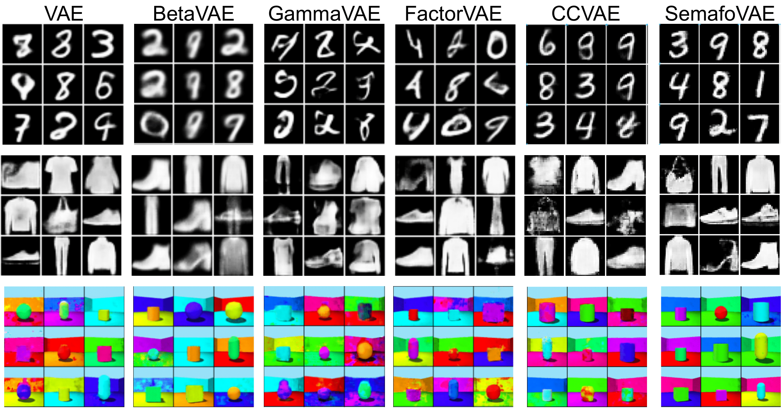
Refer to caption
Figure 10: Randomly sampled images using the prior distribution of the latent units. SemafoVAE generates shaper images than any existing methods.

A.9.3 Comparing the traverse of the latent posterior distribution

The posterior traverse experiment is performed by selecting a random example from the test set, then extracting its latent representation. Next, we linearly traverse each latent dimension from 2.5σfragments2.5σ-2.5\sigma to 2.5σfragments2.5σ2.5\sigma around its mean value and using the decoder for reconstructing the images. For all the posterior traverse figures, we select the top 6 most variate latent dimensions that correlated to the ground truth factors. Results are showed in Figure 11, Figure 12 and Figure 13.
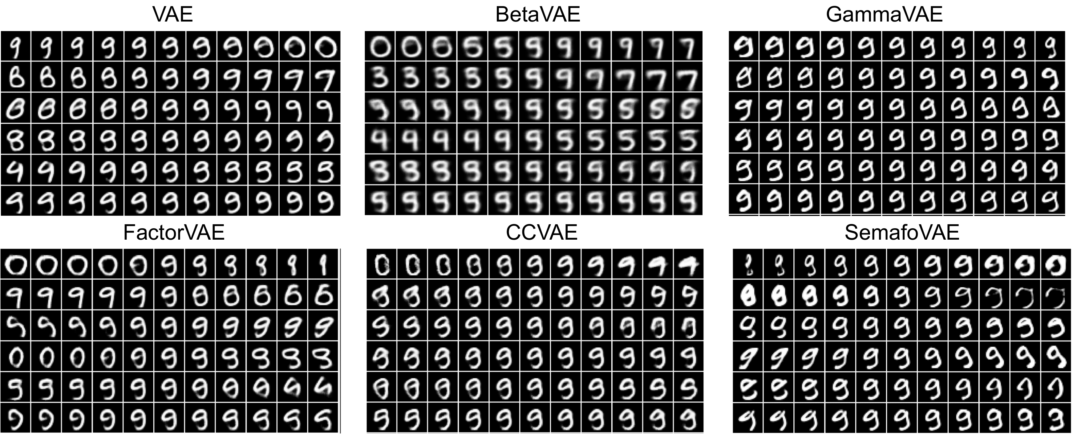
Refer to caption
Figure 11: Posterior traverse on MNIST dataset. Both CCVAE and SemafoVAE were able to capture the style of number “9”, however, SemafoVAE learns more factor of variation of the given number.
Refer to caption
Figure 12: Posterior traverse on Fashion MNIST dataset. All unsupervised methods cannot disentangle the type of clothes from the style of clothes. SemafoVAE can capture distinguished features of a “trouser” (the first row interestingly shows the traverse from a sport tight to a disco jean).
Refer to caption
Figure 13: Posterior traverse on Shapes3D dataset. All unsupervised methods show a certain level of disentanglement which encapsulate more than one factor into a single latent dimension. Both CCVAE and SemafoVAE can disentangle the factors, i.e. the shape remains invariant during the traverse while scale, orientation, wall hue, floor hue, and object hue are changing. Notably, only the semi-supervised methods capture the room orientation in the traverse (third row for CCVAE and sixth row for SemafoVAE).

A.9.4 Comparing the traverse of latents’ prior distribution

For this experiment, a random sample is drawn from the prior distribution. Then we use this vector as a reference and applying linear traversal for each of it dimension which results in a series of new latent representation. Finally, we use the decoder to reconstruct the image from the traverse vectors. For MNIST and Fashion MNIST, since we cannot know in advance which class will be generated using the unsupervised method, we perform sampling until we saw the class of interest (“9” for MNIST and “trouser” for Fashion MNIST). For Shapes3D, no particular filtering was performed, as a result, the images show different objects with different factors of variation. Results are showed in Figure 14, Figure 15 and Figure 16.

Since CCVAE has two latent spaces for style and class, we only perform prior traverse on the prior distributions of style latents.
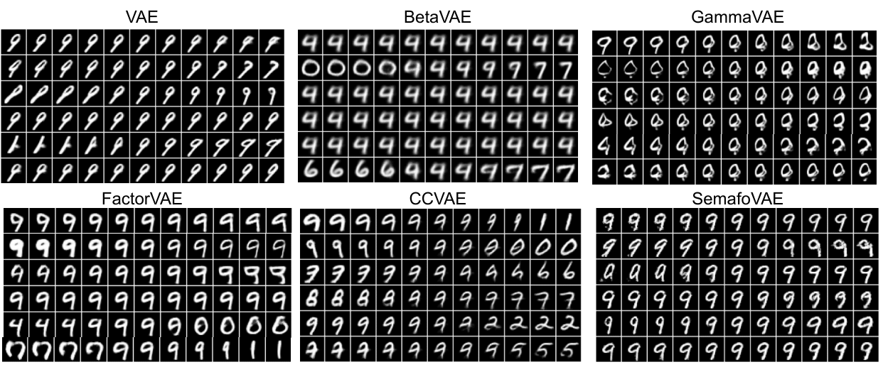
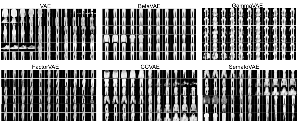
Refer to caption
Figure 14: Traverse on the latents’ prior distribution for MNIST dataset. All unsupervised methods show a mixing of styles and digits during the traverse of all dimensions. CCVAE shows certain variations in digit style, however, the images are transformed into different numbers at the end of the spectrum. SemafoVAE shows consistently in the presented number while traversing the styles of number “9”.
Refer to caption
Figure 15: Traverse on the latents’ prior distribution for Fashion MNIST dataset. FactorVAE is the only unsupervised method that captured style variations of the trouser without confusing the label. Both CCVAE and SemafoVAE show class confusion when traversing too far from the mean values.
Refer to caption
Figure 16: Traverse on the latents’ prior distribution for Shapes3D dataset. SemafoVAE shows the best quality images, and is the only method able to capture object-orientation (the fifth row) separately from the room orientation (the fourth row).
Conversion to HTML had a Fatal error and exited abruptly. This document may be truncated or damaged.