An Empirical Eye-Tracking Study of Feature Model Comprehension

Abstract.

Software Product Lines (SPLs) are families of related software systems which are distinguished by the set of features each system provides. Feature Models are the de facto standard for modelling the variability of SPLs because they describe the features, their relations, and all the combinations of features that constitute a SPL. Because of their key role, feature models are at the core of many tasks in SPL engineering. Our work presents an empirical study on the comprehension of feature models for the task of checking the validity of configurations. Our study explored the relation between the number of features and the number of cross-tree constraints with the accuracy of participants’ answers to validity checking questions, and used eye fixations for analyzing the difficulty in interpreting fixated information and the amount of cognitive processing of the different parts of the feature model stimuli. We found that answer accuracy does not relate individually to the number of features or to the number of cross-tree constrains of a feature model, but both factors do show an interaction on accuracy. Additionally, our study identified differences in feature models with cross-tree constraints in both number of fixations and fixation time, but no differences in those models without cross-tree constraints.

1. Introduction

Feature models are the de facto standard to represent the features and their combinations whose implementations is used for constructing the set of similar software systems that constitute a Software Product Line (SPL). Feature models play a crucial role throughout the development cycle of SPL (Pohl et al., 2005; Apel et al., 2013; Capilla et al., 2013). Despite their importance, the study of comprehension of these models is an area that remains largely unexplored. One of the most common tasks performed with feature models is checking that a given configuration, i.e. a combination of features, satisfies or not all the constraints expressed by a feature model. In other words, checking whether a configuration is valid or not. Despite the enormous progress in automating the support for this and other similar analysis tasks (Thüm et al., 2014; Galindo et al., 2019), all of them are ultimately driven by SPL developers who must look at a feature model and comprehend its meaning.

The goal of our empirical study is identifying some of the challenges involved in comprehending feature models, more concretely it focuses on the impact that the number of features and the number of cross-tree constraints (see definitions in Section 2.1) have on the comprehension of feature models for answering questions on the validity of configurations. More specifically, our study: i) explores the relation of these two feature model metrics with the accuracy of responses and the response time, and ii) uses eye fixations as an estimation of the cognitive effort taken by the different stimuli components of the tasks.

For our experimental design, we calculated the number of features and number of cross-tree constraints for 882 feature models taken from the largest repository available. We divided the whole dataset of feature models into four ranges for number of features and 3 ranges for cross-tree constraints, based on the distribution of these metrics along their quartile values. We obtained a random sample of 2 feature models for each of the twelve factor combinations, yielding a total of 24 feature models for which we anonymized their feature names and devised a validity checking question of similar complexity. We recruited 17 participants each of them followed a different random order of tasks.

Among other findings, our results show that the accuracy of the answers does not relate individually to the number of features or to the number of cross-tree constrains of a feature model. Instead, both of these factors show an interaction in accuracy. More strikingly, we found that looking more frequently or longer at the feature model increases the likelihood of providing an incorrect answer, irrespective of both the number of features and the number of cross-tree constraints. We argue that our work opens several avenues of research on the comprehension of feature models for configuration and other related tasks.

2. Background

In this section, we present the basic concepts and terminology of Software Product Lines and Feature Models necessary to follow our empirical study. We introduce a running example that we use to illustrate and explain our study throughout the paper, and we define the core terms related to eye-trackers studies in software engineering.

2.1. Software Product Lines and Feature Models

As mentioned before, Software Product Lines (SPLs) are families of related systems whose members are distinguished by the set of features they provide (Batory et al., 2004; Pohl et al., 2005). There exist an extensive body of research and application of SPL principles that attests the benefits that SPLs provide (e.g. (Pohl et al., 2005; Heradio et al., 2016; Galster et al., 2014; Chen and Babar, 2011)).

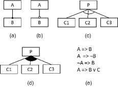
In a Software Product Line, each software product is characterized by a different combination of features. All the possible feature combinations (that correspond to all the software products) are expressed by variability models for which there are different alternatives (Czarnecki et al., 2012); however, feature models have become the de facto standard (Kang et al., 1990). In this type of model, features are depicted as labelled boxes and their relationships as lines, collectively forming a tree-like structure. The typical graphical notation and a basic textual notation of feature models is shown in Figure 1.

Figure 1. Feature Models – (a) Mandatory feature, (b) Optional Feature, (c) Alternative group, (d) Or group, (e) basic Cross-Tree Constraints

A feature is selected when it is present in a software product. A feature can be classified as:

• Mandatory which is selected whenever its parent feature is also selected. For instance, in Figure 1(a), if feature A is selected then feature B must be selected. Mandatory features are denoted with a filled circle on their end of the relationship line with their parent feature.

• Optional which may or may not be part of a product whenever its parent feature is selected. For example, in Figure 1(b), if feature A is selected, then feature B may or may not be selected. This means that there can be some software products with feature B and some others without it. Optional features are denoted with an empty circle on their end of the relationship line with their parent feature.

Features can be grouped into two ways:

• Alternative group whereby if the parent feature of the group is selected, exactly one feature from the group must be selected. For example, Figure 1(c), if feature P is selected, then exactly one of the group features C1, C2 or C3 must be selected. This means that the SPL with this group contains some software products with feature C1 selected, some with feature C2 selected, and some with feature C3 selected. However, no software product of this SPL can have more than one of these 3 features selected as they are mutually exclusive. Alternative groups are denoted with an empty arc across the lines that relate the parent and the children features.

• Or group whereby if the parent feature of the group is selected, then at least one features from the group can be selected. For example, Figure 1(d), if feature P is selected, one or more features among C1, C2 or C3 must be selected. This means that the SPL with this group can have products with one, two, or three of these features selected. Or groups are denoted with a filled arc across the lines that relate the parent and the children features.

In addition to hierarchical parent-child relations explained above, features can also relate across different branches of the feature model with Cross-Tree Constraints (CTCs) (Benavides et al., 2010; Benavides, 2019). CTCs can be denoted graphically or using propositional logic formulas because it is a common underlying formal representation for the analysis of feature models  (Benavides, 2019). We chose the propositional logic formulas because it is the format used by the FeatureIDE tool (Meinicke et al., 2017), that we used to render the visual stimuli for our empirical study as explained in Section 3.3.

We employ only a few basic forms of constraints based on the random sample of feature models selected for our empirical study. More details on the selection of feature models is presented in Section 3.2. Our empirical study considers basic CTCs expressed with a logical implication of the form $\alpha=>\beta$. We refer to the term $\alpha$ as the antecedent of the implication. Our study considers the following four forms:

• A => B. This form means that if feature A is selected, then feature B must also be selected.

• A => ¬B. This form means that if feature A is selected, then feature B must not (symbol ¬) be selected.

• ¬A => B. This form means that if feature A is not selected, then feature B must be selected.

• A => B $\vee$ C. This forms means that if feature A is selected, then (as denoted by the $\vee$ operator), either feature B, or feature C, or both must be selected.

Finally, because feature models are tree-like structures, they have a root feature that is always selected in all the products that conform a SPL. In the next subsection, we provide a running example to illustrate these concepts and our study design in Section 3.

Figure 2. Running Example – Laptop Product Line

Feature Model with our Running Example

2.2. Running Example Description

We use as a running example a fictitious product line of laptop configurations because it is a domain that is familiar to everybody. This example allows us to illustrate all the notations and concepts used in our empirical study without any loss of generality when applied to the realm of software.

Figure 2 shows the feature model of our running example. This figure was produced with the FeatureIDE tool. In this product line, a laptop computer is denoted with feature Laptop and has:

• A processor, denoted with mandatory feature Processor. In turn, the laptops can have only one type of processors, represented as an alternative group with the following features: Celeron, Corei7, and Razer.

• A hard drive, denoted with mandatory feature HardDrive. In turn, the laptops can have one or two hard drives, which is denoted by an or group with the following features: hard drive of 256GB represented by feature GB256, and hard drive with 512GB represented by feature GB512.

• Optionally has a touchscreen, denoted with optional feature Touchscreen. Hence there are laptops in the product line that have touchscreens and some that have not. For those that have touchscreens, they come with a pen to write with, denoted with mandatory feature Pen. Hence, if a laptop has a touchscreen then it must have a pen.

• RAM memory, denoted with mandatory feature RAM. The laptops can have one of three different memory sizes, which are denoted by an alternative group. The options are: 8GB represented by feature GB8, 16GB represented by feature GB16, and 32GB represented by feature GB32.

• A graphics card, denoted with feature GraphicsCard. The laptops can have only one type of graphics card, which is represented by an alternative group. The options are the following features that correspond to three types of graphics cards: GeForce, Intel, and Radeon.

In addition to the constraints that derive from the structure of the feature model, our running example also contains the following cross-tree constraints (CTCs):

1. Celeron => GB8. This CTC means that if a laptop has a Celeron processor then it must have 8GB of RAM, i.e. feature GB8 must be selected.

2. Corei7 => ¬GB16. This CTC means that if a laptop has a Corei7 processor, then it cannot have a RAM size of 16GB, i.e. feature GB16 must not be selected.

3. ¬Touchscreen => GeForce. This CTC means that if a laptop does not have a touchscreen (i.e. feature Touchscreen is not selected), then it must have a GeForce graphics card (i.e. feature GeForce must be selected).

4. Razer => GB8 $\vee$ GB16. This CTC means that if a laptop has a Razer processor, then it can either have RAM of 8GB or (operator $\vee$) 16GB, i.e feature GB8, or feature GB16, or both must be selected.

2.3. Full and Partial Configurations — Definitions and Examples

One of the principal tasks that require feature models is configuring a product, that is, defining which features are selected and which are not selected. This configuration task is the focus of our empirical study. Let us now provide working definitions and examples of the terminology we use in our study.

A configuration is defined as a set of features selected from a feature model. A configuration can be a full configuration if it considers all the constraints of an entire feature model, or can be a partial configuration if it only considers a subset of the constraints of a feature model. Recall that the constraints are those inferred from the hierarchical structure of the feature model (e.g. that only one feature from the alternative group of Processor can be selected) and those written as cross-tree constraints (e.g. if Celeron is selected then GB8 must be selected).

Configurations can be valid or invalid if they satisfy or not their set of constraints. Thus a valid full configuration meets all the constraints of an entire feature model and conversely an invalid full configuration does not meet all the constraints of an entire feature model. Similarly for partial configurations. A valid partial configuration meets all the constraints of a subset of the feature model and conversely an invalid partial configuration does not meet all the constraints of a subset of a feature model. The verification of the validity of a configuration, be it partial or full, is defined as the process of checking that all the applicable constraints, hierarchical and cross-tree, are met or not. Let us now provide examples of the verification of the validity of four configurations (two full and two partial).

As a first example, please consider the following full configuration with the selected features {Laptop, Processor, Celeron, HardDrive, GB256, Touchscreen, Pen, RAM, GB8, GraphicsCard, Intel}. Let us first verify the constraints derived from the structure of the feature model. The root feature Laptop is selected, as well as all its mandatory child features: Processor, HardDrive, RAM, and GraphicsCard. Furthermore, optional feature Touchscreen and its mandatory child feature Pen are both correctly selected. Notice also that only one processor is selected (feature Celeron), one hard drive size is selected (feature GB256), one RAM size is selected (feature GB8), and one graphics card is selected (feature Intel). Now let us focus on the cross-tree constraints. The first CTC is met because feature Celeron is selected and GB8 is also selected. The second CTC refers to Corei7 in the antecedent of the implication, and because it is not selected (i.e. false) the constraint is met. Similarly for the third CTC, because the Touchscreen feature is selected (i.e. true) the antecedent does not hold and the constraint is met. Similarly also for the fourth CTC whose antecedent is feature Razer, which is not selected and hence the constraint is met. Because this configuration meets all the constraints of the feature model it is a valid full configuration.

As a second example, consider the following full configuration with the selected features {Laptop, Processor, Corei7, HardDrive, GB512, Pen, RAM, GB16, GraphicsCard, Intel}. Following a similar process as described for the hierarchical constraints of the first example, it is simple to verify that all these constraints are met except one. Namely, feature Pen is selected but its parent feature Touchscreen is not selected. This constraint violation alone is enough to render this configuration as an invalid full configuration. Nonetheless, let us analyze the cross-tree constraints. The first CTC is met because the antecedent of the implication refers to feature Celeron which is not selected. The second CTC is violated because feature Corei7 is selected and GB16 is also selected in the configuration, situation that is prohibited by this CTC. The third CTC is also violated because given that feature Touchscreen is not selected, this constraint required that feature GeForce were selected, but it is not. The fourth CTC is met because the antecedent refers to feature Razer which is not selected. In summary, this full configuration is invalid because it violates three constraints, one from the hierarchy of the feature model and two cross-tree constraints.

As a third example, consider the following partial configuration with the selected features Razer, HardDrive, GB256, GB512, Touchscreen, GB8, GeForce. Because it is a partial configuration, for its validity we only need to verify the constraints where these features are involved. As before, we verify the hierarchical constraints. Feature Razer is selected and there are no other hierarchical constraints to check for it. Features HardDrive, GB256, and GB512 belong to the same or group, hence the constraints of this type of group are met. Touchscreen is a feature that can be selected and there are no other constraints to verify as neither the feature Laptop nor the feature Pen are in the set of features of this partial configuration. Similarly, for features GB8 and GeForce there are no other hierarchical constraints to validate as the features they relate to are not selected in the partial configuration. Regarding the CTCs, the first CTC is relevant because it refers to feature GB8. However, because feature Celeron is not in the partial configuration (hence false), the CTC is met. The second CTC is not relevant as it does not involve any of the features of the partial configuration. The third CTC is relevant because it refers to two features in the partial configuration. However, because feature Touchscreen is actually selected the antecedent of the implication does not hold and hence the CTC is met. The fourth CTC is met because feature Razer and feature GB8 are selected in the partial configuration. In summary, this is an example of a valid partial configuration as it meets all constraints of its subset of the feature model.

As a final example, consider the following partial configuration with the selected features {Corei7, Touchscreen, RAM, GB16, GB32, Intel}. Again, because it is a partial configuration we need to verify only the constraints where these features are involved. Feature Corei7 is selected and there are no other features that relate to it in the structure of the feature model. Similarly, feature Touchscreen is selected and none of the features it relates to are in the partial configuration. Thus both features meet their subset of hierarchical constraints. Now left focus on the alternative group of feature RAM and the two members of the group, feature GB16 and feature GB32, both of which are selected in the partial configuration. This is a clear violation of an alternative group which requires that only one feature in the group can be selected. This violation alone is enough to render make the partial configuration invalid. Nonetheless, let us look at the remaining subset of constraints that need to be verified. Feature Intel is selected but no other feature it relates to are in the partial configuration, thus its constraints are met. Now regarding the CTCs, the first one is not relevant because it does not reference any feature in the partial configuration. The second CTC is violated because Corei7 is selected but feature GB16 is also selected. The third CTC is met because the antecedent of the implication does not hold as feature Touchscreen is in the partial configuration. The fourth CTC is met because the antecedent of the implication is not in the partial configuration. In summary, this is an invalid partial configuration.

2.4. Eye-tracking Basics

There is an extensive and long standing body of research in eye-tracking theory and practice (e.g. (Duchowski, 2017; Holmqvist and Andersson, 2017)). Among this research, there is a vast number of works in the area of software engineering as summarized, for example, by Obaidellah et al.  (Obaidellah et al., 2018), and Sharafi et al.  (Sharafi et al., 2015, 2020). Eye tracking is based on the visual attention of participants whose eye gaze data is recorded. The premise is that visual attention triggers the cognitive processes required for the comprehension and resolution of tasks, and in turn such cognitive processes direct the visual attention to specific locations on the visual field of the participant.

As defined by Sharafi et al., a visual stimulus is any object required to perform a task whose visual perception triggers the participant’s cognitive processes to perform some actions related to the task (Sharafi et al., 2020). Because our study focuses on feature models and their comprehension, they are at the core of our visual stimuli. Section 3.3 provides further details on the stimuli definition. Our empirical study focuses on fixations which are eye movements that stabilize the retina on an object of interest in a visual stimulus (Duchowski, 2017). The duration of the fixations varies by the task performed and the participants, with typical values can range from 100 to 400 milliseconds (Duchowski, 2017; Holmqvist and Andersson, 2017).

An Area Of Interest (AOI) is an area in the visual stimulus where the researcher is interested in gathering data about because they are deemed relevant for performing the participants’ tasks (Holmqvist and Andersson, 2017). AOIs are used to defined third order data, according to Sharafi’s et al. data classification  (Sharafi et al., 2020). In particular, our study considers two third order data: 1) fixation count which is defined as the number of fixations on a specific AOI, 2) and fixation time which is defined as the aggregated duration of all the fixations on a specific AOI. In our study, we defined multiple AOIs based on the semantics of the feature models and used ratios of these two measures to normalize the data across participants and questions (Holmqvist and Andersson, 2017). Further details on the AOIs and their relation to the research questions are provided throughout the coming section.

3. Empirical Study Design

In this section, we state our research questions and provide their rationale, we describe the process to select the feature models of our study, and how we constructed the visual stimuli from them. Furthermore, we describe our experimental design, including the selection of participants and assignment of experimental conditions.

3.1. Goal and Research Questions

As mentioned before, there is an extensive research on metrics of feature models (El-Sharkawy et al., 2019). Our empirical study focuses on two of the most basic metrics namely, Number of Features (NoF) and Number of Cross-Tree Constraints (NoC). We state our research goal as follows:

Goal. To analyze the impact of the metrics Number of Features (NoF) and Number of Cross-Tree Constraints (NoC) in the comprehension of feature models for the task of verifying the validity of full and partial configurations.

Henceforth, for sake of brevity, whenever we refer to verification tasks we imply the verification of the validity of configurations. The research questions of our empirical study are the following:

RQ1. Is there any effect of NoF and NoC on the accuracy of verification tasks? Rationale: This question examines the effect of NoF, and NoC on the accuracy of the response to a verification task.

RQ2. Is there any effect of NoF and NoC on the response time of verification tasks that were answered correctly? Rationale: The purpose of this question is to identify for the tasks answered correctly whether or not there is an effect of NoF or NoC.

RQ3. Can the accuracy of verification tasks be inferred from the ratios of fixation counts within specific AOIs of feature models’ stimuli? Rationale: The ratios of fixation counts within the AOIs of a feature model can be interpreted as a proxy of the cognitive effort taken for the comprehension of such AOI during a verification task. We want to find out if this proxy can be used to infer the accuracy of responses.

RQ4. Can the accuracy of verification tasks be inferred from the ratios of fixation time within specific AOIs of feature models’ stimuli? Rationale: Similar to the previous question, we want to find out if the ratio of fixation time within the AOIs of a feature model can be used to infer the accuracy of responses.

3.2. Selection of Feature Models

For our empirical study, we obtained all the 882 feature models available from SPLOT repository, which has the largest dataset of publicly available feature models. With the provided SPLOT API, we implemented the feature metrics NoF and NoC and applied them to our dataset. Table 1(b)(a) shows the minimum, maximum, and mean values as well as the first, second and third quartile values of our metrics NoF and NoC. On closer inspection, we observed a long-tailed distribution of values of NoC. Based on our experience using feature models, we decided to set the maximum value of NoC at 15 for our study. This threshold eliminated only 35 feature models out of the original 882 models in our dataset.

We then analyzed the distribution of the feature models along the quartile values for the NoF metric. The ranges considered were: (1) Min¡=NoF¡Q1, (2) Q1¡=NoF¡Q2, (3) Q2¡=NoF¡Q3, and (4) NoF¿=Q3. For the NoC metric, we set three ranges: (1) feature models with no CTCs (i.e. NoC=0, between minimum and Q1), (2) feature models with 1 or 2 CTCs (i.e. Q1¡=NoC¡Q3), and (3) feature models with 3 to 15 CTC (i.e. Q3¡=NoC¡=15).

Table 1(b)(b) shows the number of feature models for each range combination of NoF and NoC. The highest frequency with value 114 was for feature models with between 20 to 34 features (range 3 in NoF dimension) and without CTC (range 1 in NoC dimension). The lowest frequency with value 29 was for feature models with 10 to 13 features (range 1 in NoF dimension) and 3 to 15 CTC (range 3 in dimension NoC). As a final step, for our empirical study we randomly selected two feature models for each combination of ranges along both dimensions . The details of the 24 feature models selected and their NoF and NoC are in our replication package.

Table 1. Feature Model Selection Summary

(a) (a) Descriptive statistics, N=882

Metric	Min	Q1	Q2	Mean	Q3	Max
NoF	10	14	20	27.95	35	366
NoC	0	0	1	3.531	3	246

(b) (b) Feature models per range of NoF and NoC, N=847

		NoF
		(1) 10..13	(2) 14..19	(3) 20..34	(4) ¿=35
NoC	(1) 0	106	93	114	78
	(2) 1..2	73	88	40	34
	(3) 3..15	29	27	77	88

Ranges for NoF:1,2,3,4 Ranges for NoC: 1,2,3

3.3. Tasks and Stimuli Selection

We define a task for each feature model in our sample. A task consist of answering a validity verification question that has one of the following two forms, where ¡configuration¿ stands for a list of features in a feature model:

• Is ¡configuration¿ a valid partial configuration?

• Is ¡configuration¿ a valid full configuration?

Please do notice that in feature models, the names of the features are meaningful as they usually convey additional information about the relationships among features. This information could be used while executing tasks with the feature models and it may have a positive or negative effect on the performance depending on the familiarity of the participants with the domain of the feature models. Hence, we anonymized the features’ names to prevent any such effect by renaming the features with sequences of letters in alphabetical order and increasing length following a breadth-first traversal order of the feature model.

For the selection of the questions, we considered a length of six features and favoured full configurations over partial configurations. In some cases, it was necessary to consider more or less features to provide meaningful questions. In summary, 17 questions use a partial configuration and 7 questions a full configuration. Regarding the number of features in the configurations, 14 questions have 6 features, four questions have 7 features, two questions have 3 features, two questions have 8 features, one question has 5 features, and one question has 10 features.

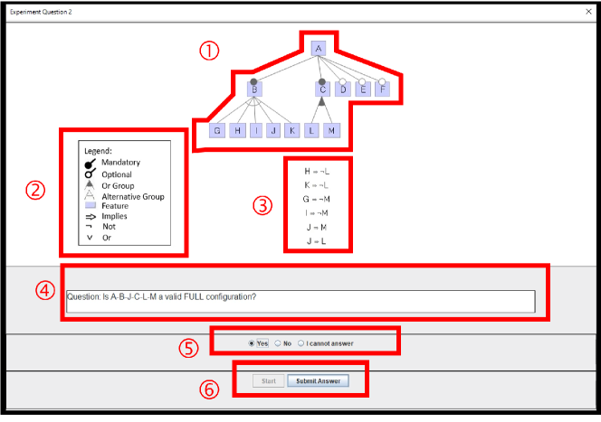
We also aimed at balancing the distribution of the features that are part of the configuration question across the feature models. This means that we selected the features of the configuration questions in different areas along the horizontal axis (i.e., left, middle, right) and the vertical axis (i.e., top, middle, bottom). As an example, Figure 3 shows a full configuration question involving 13 features and 6 CTCs. Notice also that for readability we separated the features in the configuration with a dash (–) rather than with commas. In this figure, three of the features are leaves on the tree-structure, two are children of the root feature, and half of the features appear to the left of the root and half to the right.

Figure 3. Stimulus Example – Java graphical interface with superimposed Areas of Interest (AOIs): ➀ feature model (FM), ➁ legend label (Label), ➂ cross-tree constraints area (CTC), ➃ question panel (Question), ➄ answer panel (Answer), and ➅ buttons panel (Buttons).

Stimulus example of configuration question with AOIs

We explored different alternatives to present the stimuli of our study, among them iTrace and PsychoPy. However, it was not possible to link FeatureIDE, which is an Eclipse plugin, with them to allow us to obtain the information required for our study. Therefore, we wrote a bespoken Java program that presents a configurable sequence of questions, like that of Figure 3.

The program provides a simple user interface with the following elements: i) the feature model, ii) a legend that summarizes the notations, iii) area for cross-tree constraints of the form presented in Section 2.1, iv) a question panel where the question is presented, v) an answer panel that shows the three possible answers Yes, No, and I cannot answer (given to participants to indicate that they were not able to respond), and vi) a response panel with the buttons to start answering the question and submitting the answer. The program records the responses and the response time. The feature model appears once the participant hits the Start button and the response time clock gets started. The response time ends when the participant hits the Submit Answer button which also clears the feature model for the next question.

3.4. Experimental Design

We followed the guidelines proposed by Sharafi et al. for planning and executing our empirical study (Sharafi et al., 2020). We chose a within-subjects design where each participant performed the 24 tasks, each task being a validity verification question as described above. In addition, we randomized the order of the tasks in such a way that each participant follow a different order (Lazar et al., 2017).

We recruited 19 participants, two of them piloted our experimental design, mostly graduate students from our institution and without prior knowledge of feature models. We created a tutorial video to fill this background gap. The video is an extended and detailed version of the contents presented from Section 2.1 to Section 2.3. This video has a duration of about 40 minutes and was presented to each participant right before the start of his/her tasks.

We performed our study in a research lab devoted to user studies at our institution, where a participant is alone in the experiment room and the experimenter is at an adjacent observation room overseeing the experiment. This arrangement guaranteed a stable and regular environment without any distractions, with controlled factors such as lighting of the room and position of the participants in relation to the screen, keyboard and eye-tracker. For our study, we used the Tobii Pro Fusion bar eye-tracker and Tobii Pro Lab tool for capturing and analyzing the data. The session of each participant followed the sequence:

• Brief introduction of the experiment by the experimenter, describing its goal and the protocol to follow.

• Signing the consent form in accordance with the ethics certificate of our institution.

• Watching training video and clarifying any questions or issues that the participants may have.

• Calibration of the eye-tracker using Tobii Pro Lab tool.

• Warm-up practice with two questions in the Java application (see Section 3.3) to gain familiarity with the graphical interface.

• Semi-structured interview to gather further insights from the participants. The interviews were recorded for subsequent analysis.

More formally, our empirical study is a factorial design with two factors that correspond to our independent variables (Wohlin et al., 2012). The first factor is Number of Features (NoF) with 4 categorical values, and the second factor is Number of Cross-Tree Constraints (NoC) with 3 categorical values, respectively corresponding to their number of ranges as explained in Section 3.2.

Recall that our Java interface collects two pieces of information for each question: i) correctness, with values true and false to indicate whether the response was correct or not, and b) response time in milliseconds, i.e. the elapsed time between clicking on the Start button and hitting the Submit Answer button. Thus, these are our first two dependent variables, respectively in nominal and ratio scales. They are used for answering our first two research questions, RQ1 and RQ2.

With the aid of Tobii Pro Lab, we defined several areas of interest (AOIs) on top of the Java interface, see Figure 3. The AOIs roughly correspond to the elements in the graphical interface: ➀ feature model (FM), ➁ legend label (Legend), ➂cross-tree constraints area (CTC), ➃ question panel (Question), ➄ answer panel (Answer), and ➅ buttons panel (Buttons). We should note that the AOI that corresponds to the feature model, i.e.  ➀ in the figure, is tailored to each of the 24 feature models we used in our study. Similarly, the area of interest of CTCs, ➂ in the figure, was removed when there were no CTCs and adapted according to the number of CTCs of the feature model. The rest of the graphical elements were fixed on the same area of the interface across all questions. For all our AOIs, we collected the fixations count and the fixation time on them. We normalized these values as percentages to analyze across questions and participants (Holmqvist and Andersson, 2017). We used these data for the research questions RQ3 and RQ4.

4. Results and Analysis

In this section, we start with a general overview of the results obtained before delving into the detailed analysis for each of our four research questions.

4.1. Descriptive Statistics

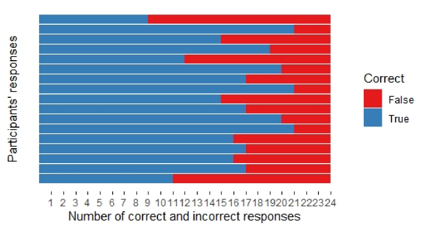
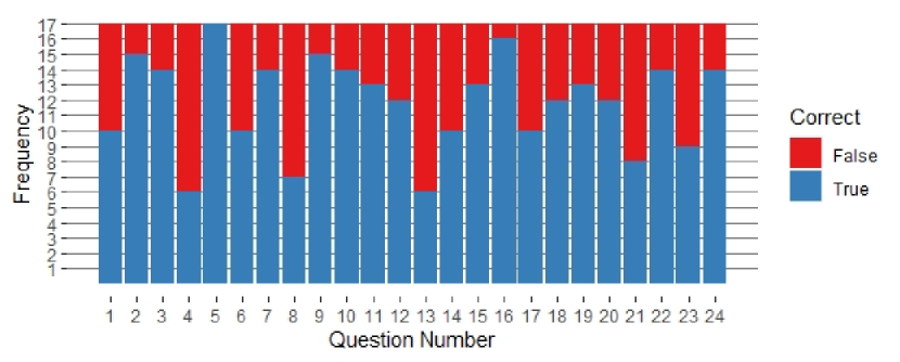
Our empirical study had 17 participants, 10 male and 7 female. All participants completed the 24 questions, and only one participant in one question indicated that he/she could not answer the question. Figure 4(b) summarizes the correct and incorrect responses per participant and per question.

Figure 4(a) shows for each participant the number of correct and incorrect responses. In total for all participants, there were 284 correct and 124 incorrect answers. Participants had between 9 to 21 correct answers, with a median of 17, and conversely they had between 3 and 15 incorrect answers with a median of 7. On average, the correct answers took 42.84 seconds to respond with a standard deviation of 26.15 seconds. For the incorrect answers, the average response time was 52.96 seconds, with a standard deviation of 37.82 seconds. Figure 4(b) shows the distribution of correct and incorrect answers per question. The minimum was six correct answers for questions 4 and 13, and the maximum was 17 for question 5 which all the participants answered correctly. The average was 11.83 correct answers per question with a standard deviation of 3.08.

(a) Correct/Incorrect responses per participant

(b) Correct/Incorrect responses per question

Figure 4. Summary of correcct and incorrect responses

Descriptive Statistics

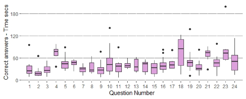
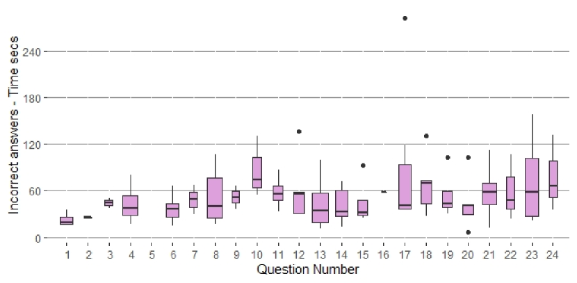
Figure 5(b) summarizes the distribution of response time per question for correct and incorrect answers. Figure 5(a) shows the distribution of response time of correct answers per question. Notice that only four questions have their third quartile above one minute. One question above this threshold is question 4 which was one with the least number of correct answers. In contrast, Figure 5(b) shows the distribution of response time of incorrect answers per question. For the majority of the questions, the distribution is more widely spread, with only 3 questions whose their third quartile was over the one minute threshold.

(a) Response time distribution of correct answers

(b) Response time distribution of incorrect answers

Figure 5. Response time distribution per question

Descriptive Statistics

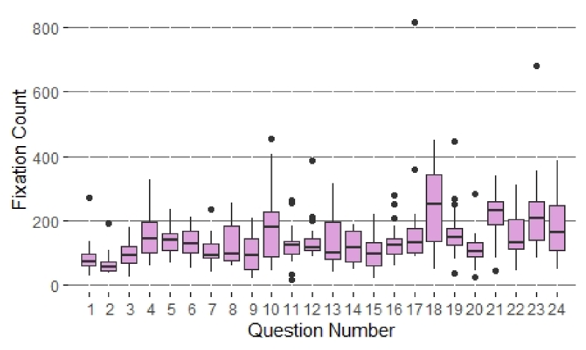
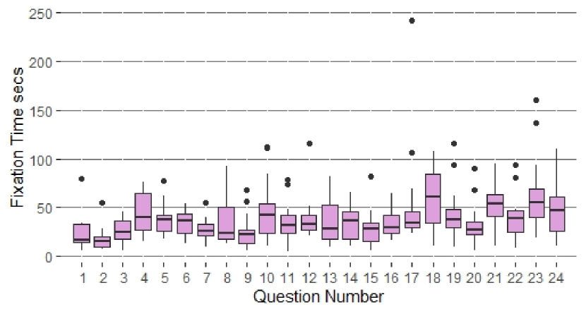
Figure 6(b) summarizes our findings in terms of fixation count and fixation time per question. Across all participants, the quartile values for fixation counts were: 84, 124, and 184. The minimum value was 18, the maximum value was 817 and the standard deviation was 92.31. Along the same lines, the quartile values of fixation time per question were: 21.11 sec, 32.5 sec, and 48.05 sec. The minimum value was 5.14 sec, the maximum 242.29, and the standard deviation of 25.85 sec. Figure 6(a) shows the distributions of fixation count per question. Except for questions 18, 21, 23, and 24, all the other questions have median values below 200 fixations. Notice as well the presence of outlier values, in particular in question 17 and question 23. Figure 6(b) shows the aggregated fixation time per question. This figure follows a similar pattern with the same questions having medians above 50 seconds of total fixation time.

(a) Fixation count per question

(b) Total fixation time per question

Figure 6. Fixations count and fixation time per question

Fixations count and fixation time per question

Recall that in Section 3.3, we identified six AOIs in the stimuli corresponding to each question of our study. Figure 7(b) shows the results of fixation count and fixation time by AOI. Figure 7(a) shows a stratified histogram of the ratio on the number of fixations per question grouped by AOI. The values of the mean and standard deviation for each AOI are as follows: Feature Model ($\overline{x}=45.27$, $s=15.97$), Question ($\overline{x}=31.66$, $s=10.50$), CTC ($\overline{x}=7.273$, $s=8.76$), Answer ($\overline{x}=4.37$, $s=3.08$), Legend ($\overline{x}=3.11$, $s=3.51$), and Buttons ($\overline{x}=2.05$, $s=1.93$). All these values are reflected in the figure, whereby the histogram values of the feature model (FM) appear at the rightmost part of the graph, followed to the left by the histogram values of the Question and CTC AOIs respectively. The ratio contribution of AOIs Buttons, Legend and Answer were rather small as depicted with the highest frequency on the left of the graph. A very similar scenario was observed on the ratio of fixation time per question grouped by AOI shown in Figure 7(b). The values for this figure are: Feature Model ($\overline{x}=46.19$, $s=16.87$), Question ($\overline{x}=30.66$, $s=10.93$), CTC ($\overline{x}=7.252$, $s=9.18$), Answer ($\overline{x}=5.693$, $s=043.70$), Legend ($\overline{x}=2.66$, $s=3.64$), and Buttons ($\overline{x}=2.67$, $s=2.64$). Here again, the histogram values of the feature model (FM) have the highest ratios values to the right of the graph, followed by Question and CTC. Once again, the highest counts were for AOIs Legend, Answer and Buttons.

(a) Ratios of fixations count per question grouped by AOI

(b) Ratios of fixation time per question grouped by AOI

Figure 7. AOI fixation count and fixation time results

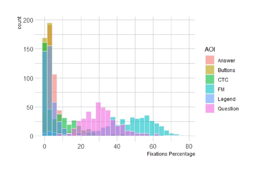
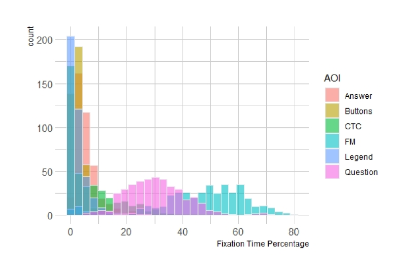
AOI fixation count and fixation time results

4.2. RQ1 results

Recall from Section 3.1 that this question aims at identifying any effects of NoF and NoC on task accuracy. Hence, the independent variables are the NoF and NoC that are of categorical scale, and the dependent variable is task accuracy (with correct and incorrect values). To answer this question, we used multiway frequency analysis whereby the frequency of a cell (i.e., a combination of factors) is the dependent variable that is influenced by one or more categorical factors and their associations  (Tabachnick and Fidell, 2013). In this method, the null hypothesis $H_{0}$ is that the factors do not affect the frequency distribution of a dependent variable.

Our results show that there are neither main effects of NoF nor of NoC on task accuracy. However, there is an interaction effect of NoF and NoC on task accuracy ($\chi^{2}_{6}=21.82$, $p<.001$). The higher the value of NoC caused a lower task accuracy, but this drop is different across the values of NoF. This pattern of results can be interpreted as an indication that the value of NoC imposes more cognitive challenges than the value of NoF.

4.3. RQ2 results

Recall from Section 3.1 that for this question, we are interested in the effect of NoF and NoC on the response time of tasks answered correctly. An ANOVA test was used to establish the effect of two categorical factors, NoF and NoC, on a continuous dependent variable, response time. The null hypothesis $H_{0}$ is that the means across both factors and their interaction are equal (Tabachnick and Fidell, 2013). For correct answers, both NoF ($F_{3,272}=8.28$, $p<0.001$, $\eta^{2}_{p}=0.084$) and NoC ($F_{2,272}=11.58$, $p<0.001$, $\eta^{2}_{p}=0.078$) have a main effect on response time. There is not interaction effect of NoF and NoC on response time. NoF causes an almost steady increase in time needed to answer correctly, and the same is true for NoC.

4.4. RQ3 results

Recall from Section 3.1, that for this question we want to find out if the ratio of fixation counts of the AOIs can be used to explain the accuracy of the responses. Consequently, the analysis focuses primarily on the accuracy of answers, with the eventual examination of interaction effects of this factor with NoF and NoC. Thus, accuracy, NoF and NoC are the independent variables and the ratios of fixation counts of the six AOIs are our dependent variables, that is, the AOIs Answer, Buttons, CTC, FM, Legend and Question as explained in Section 3.4. Because tasks with CTCs involve the additional AOI CTC, we applied the MANOVA test twice, once for the tasks with CTCs and once for the tasks without CTCs (Tabachnick and Fidell, 2013).

For tasks with CTCs, the MANOVA test considered the factors (2:accuracy x 4:NoF x 3:NoC). For this test, the null hypothesis $H_{0}$ for the omnibus test states that the factors are not related to the variance of the dependent variables taken globally. When the omnibus test is significant for one factor or a combination of factors, the null hypothesis $H_{0}$ for each dependent variable is that this factor or combination of factors is not related to the variance of any of the six dependent variables. We found from the omnibus test that the accuracy of answers was significant globally, that is, the ratio of fixation counts of each AOI is related to the accuracy of answers ($F_{6,251}=3.458$, $p<.003$, $\eta^{2}_{p}=.076$), with no interaction effect of this factor with NoF and NoC. Because of this finding, we analyzed the implication of accuracy on each of the six dependent variables. We observed significant differences in the means of the following AOIs: FM ($F_{1,256}=19.150$, $p<.001$, $\eta^{2}_{p}=.070$), CTC ($F_{1,256}=8.088$, $p<.005$, $\eta^{2}_{p}=.011$), Question ($F_{1,256}=17.723$, $p<.001$, $\eta^{2}_{p}=.065$), and Buttons ($F_{1,256}=4.032$, $p<.046$, $\eta^{2}_{p}=.016$). Differences in the means of fixation count ratios for given AOIs for correct vs incorrect responses were as follows: FM 39% vs 48%, CTC 12% vs 9%, Question 35% vs 28%, and Buttons 2% vs 1.7%. This finding means that devoting more cognitive effort in comprehending the FM AOI is related to a higher likelihood of providing an incorrect answer. Inversely, devoting more cognitive effort in understanding the AOIs CTC, Question, or Buttons is related to a higher likelihood of providing a correct answer.

For tasks without CTCs, the MANOVA test considered the factors (2: accuracy x4: NoF) because the value of CTC is now a constant. The results show that the null hypothesis of the omnibus test could not be rejected ($F_{5,124}=0.296$, $p>.05$), therefore the results for each of the dependent variables were not examined. In other words, the proportion of fixation counts of each AOI is not related to the accuracy of answers.

4.5. RQ4 results

This question is similar to the previous one, but here we want to find out if the ratio of fixation time of any AOI can be used to explain the accuracy of the responses. Thus, we answered the question in the same way but using the ratios of fixation time. Again, the tests were run separately for tasks with and without CTC because of the same reasons.

For tasks with CTC, the proportion of time fixating each AOI is related to the accuracy of answers ($F_{6,251}=3.027$, $p<.007$, $\eta^{2}_{p}=.067$). Additionally, there is no interaction effect of accuracy of answers with the experimental factors, NoF and NoC. Regarding the relation between accuracy of answers and each of the specific dependent variables (AOIs), the tests are significant for: FM ($F_{1,256}=15.952$, $p<.001$, $\eta^{2}_{p}=.059$), Question ($F_{1,256}=16.486$, $p<.001$, $\eta^{2}_{p}=.061$), and Answer ($F_{1,256}=4.796$, $p<.029$, $\eta^{2}_{p}=.018$). Differences in the means of fixation time ratios for given AOIs for correct vs incorrect responses were as follows: FM 40% vs 49%, Question 34% vs 28%, and Answer 6% vs 4%. This finding means that devoting more cognitive effort in comprehending the FM AOI is related to a higher likelihood of providing an incorrect answer. Inversely, devoting more cognitive effort in understanding the AOIs Question or Answer is related to a higher likelihood of providing a correct answer.

For tasks with no CTC, the proportion of time fixating each AOI is not related to the accuracy of answers ($F_{5,124}=0.197$, $p>.05$). Since the null hypothesis for the omnibus test could not be rejected, no further statistical analysis was required.

4.6. Threats to Validity

Our empirical study faced several potential threats to validity as similar studies that rely on eye-tracker measures (Wohlin et al., 2012; Sharafi et al., 2020). Concerning internal validity, a threat was participant selection. We addressed this issue by recruiting as large and diverse a set of participants as possible, both in terms of gender and technical knowledge of the subject. Because we used a within-subjects design we faced an order effect bias whereby participants perform better as they performed more tasks. We mitigated this threat by using a random order of tasks for each participant. The instrumentation threat concerns the quality and reliability of the artifacts used in the experiment. We tackled this threat by following a rigorous protocol that included multiple checks from eye-tracker measures and calibrations for each participant to extensive consistency manual and automated validations of the collected and synthesized data.

Regarding external validity, a fundamental threat is the selection of the feature models. Certainly, selecting other data set of feature models might yield different results from ours. However, we argue that we addressed this threat by choosing feature models from the largest repository available and in a random way across the twelve combinations of our two factors that are our feature metrics. Because the majority of our participants were graduate students without background in feature models, we cannot generalize our findings for other groups like experienced developers or variability experts. Nonetheless, this aspect is part of our future work. In terms of construct validity, we used standard measures of cognitive load such as accuracy, response time, ratios of fixation counts and fixation time on AOIs which were analyzed with standard statistics procedures (Holmqvist and Andersson, 2017; Gonçales et al., 2021). Considering other eye-tracking and multimodal measures of cognitive load are also part of our future work.

5. Related Work

There is an extensive body of research in program comprehension analyzed with eye-trackers (Obaidellah et al., 2018; Sharafi et al., 2015, 2020). In this section, we briefly summarize the pieces of work closest to ours. There are several studies that use eye-trackers on models of software. For instance, Jeanmart et al. study the impact of the presence or absence of the explicit Visitor pattern in a UML class diagram for comprehension and maintenance tasks (Jeanmart et al., 2009). They found that the Visitor pattern did not reduce the efforts for the comprehension task but instead that the familiarity with UML and patterns had an impact on both tasks. Similarly, other aspects of UML diagrams and their impact on comprehension have also been studied, e.g. color and layout (Yusuf et al., 2007).

There is an extensive and seminal line of work by Janet Siegmund and colleagues in the study of program comprehension in code with variability, studying aspects such as color, conditional compilation versus feature-oriented programming, or disciplined vs non-disciplined annotations (e.g, (Feigenspan et al., 2013; Santos et al., 2019; Schulze et al., 2013)). However, to the best of our knowledge, for this line of work they do not employ eye-tracker measures. In contrast, Melo et al. performed an experiment to understand how developers debug programs with and without variability (Melo et al., 2017). In code fragments with variability, they found increases in debugging time and in the number of gaze transitions between the use and definitions of fields and methods. Da Costa et al. studied C code with annotations and the impact of three refactorings in terms of program comprehension and visual effort (da Costa et al., 2021). They found that two of such refactorings had an impact. In contrast with these works on variability, our study uses feature models, not source code, and our task is comprehension of configuration validity rather than code debugging or refactoring.

6. Conclusions and Future Work

We presented the first empirical study on feature model comprehension using eye-tracking measures for tasks of verifying validity in partial and full configurations. Our focus was on the impact of two feature model metrics, number of features (NoF) and number of cross-tree constraints (NoC), on these verification tasks. We found that these tasks are complex from a cognitive point of view because they are affected by multiple factors. For instance, tasks with more NoF or more NoC involved more cognitive operations to answer correctly as shown by a steady increase on response time. Also, when considering the different aspects (AOIs) of the visual stimuli, our most striking finding was that looking more frequently or longer at the feature model (AOI FM) of a task increases the likelihood of providing an incorrect answer, irrespective of the NoC and NoF.

We believe our work opens several avenues for further research. Among them are: studying other eye-tracking measures of cognitive load from pupil size to EEG (Gonçales et al., 2021), employing finer grain AOIs for the feature model AOI that would permit us to identify transition patterns or navigation strategies among AOIs in the form of scan paths and conditional probabilities, analyzing the impact of other feature model metrics (e.g., branching factor), and including a larger and more diverse participant population.