On the polytropic Bondi accretion in two-component galaxy models with a central massive BH

Abstract

In many investigations involving accretion on a central point mass, ranging from observational studies to cosmological simulations, including semi-analytical modelling, the classical Bondi accretion theory is the standard tool widely adopted. Previous works generalised the theory to include the effects of the gravitational field of the galaxy hosting a central black hole, and of electron scattering in the optically thin limit. Here we apply this extended Bondi problem, in the general polytropic case, to a class of new two-component galaxy models recently presented. In these models, a Jaffe stellar density profile is embedded in a dark matter halo such that the total density distribution follows a $r^{-3}$ profile at large radii; the stellar dynamical quantities can be expressed in a fully analytical way. The hydrodynamical properties of the flow are set by imposing that the gas temperature at infinity is proportional to the virial temperature of the stellar component. The isothermal and adiabatic (monoatomic) cases can be solved analytically, in the other cases we explore the accretion solution numerically. As non-adiabatic accretion inevitably leads to an exchange of heat with the ambient, we also discuss some important thermodynamical properties of the polytropic Bondi accretion, and provide the expressions needed to compute the amount of heat exchanged with the environment, as a function of radius. The results can be useful for the subgrid treatment of accretion in numerical simulations, as well as for the interpretation of observational data.

1 Introduction

Table 1: Main properties of accretion solutions in one- and two-component galaxy models with central MBH.

	KCP16	CP17	CP18	MCP21 (this paper)
Galaxy models	Hernquist (1990)	Hernquist (1990), Jaffe (1983)	JJ models (CZ18)	J3 models (CMP19)
Type of accretion	Polytropic	Isothermal	Isothermal	Polytropic
Number of sonic points	One or two	One or two (Hernquist), One (Jaffe)	One	One or twob
Sonic radius	Analytica	Analytic	Analytic	Analytic/numericalc
$\lambdaup_{\hskip 0.56905pt{\rm t}}$	Analytica	Analytic	Analytic	Analytic/numericalc
Mach number profile	Numerical	Analytic	Analytic	Analytic/numericalc

• The general expression can be written as a function of the polytropic index, but only special cases were given explicitly;
  

• Function of the polytropic index $\gamma$;
  

• In the isothermal ($\gamma=1$) and monoatomic adiabatic ($\gamma=5/3$) cases it is analytic, in the $1<\gamma<5/3$ case only a numerical exploration is possible.

Theoretical and observational studies indicate that galaxies host at their centre a massive black hole (MBH) that has grown its mass predominantly through gas accretion (see e.g. Kormendy & Richstone 1995). A generic accretion flow may be broadly classified as quasi-spherical or axisymmetric, and what mainly determines the deviation from spherical symmetry is the angular momentum of the flow itself. A perfect spherical flow is evidently only possible when the angular momentum is exactly zero. Spherical models are a useful starting point for a more advanced modelling, and thus gas accretion toward a central MBH in galaxies is often modelled with the classical Bondi (1952) solution. For example, in semi-analytical models and cosmological simulations of the co-evolution of galaxies and their central MBHs, the mass supply to the accretion discs is linked to the temperature and density of their environment by making use of the Bondi accretion rate (see e.g. Fabian & Rees 1995; Volonteri & Rees 2005; Booth & Schaye 2009; Wyithe & Loeb 2012; Curtis & Sijacki 2015; Inayoshi, Haiman & Ostriker 2016). In fact, in most cases, the resolution of simulations cannot describe in detail the whole complexity of accretion, and so Bondi accretion does represent an important approximation to more realistic treatments (see e.g. Ciotti & Ostriker 2012; Barai et al. 2012; Ramírez-Velasquez et al. 2018; Gan et al. 2019 and references therein). Recently, Bondi accretion has been generalised to include the effects on the flow of the gravitational field of the host galaxy and of electron scattering, at the same time preserving the (relative) mathematical tractability of the problem. Such a generalised Bondi problem has been applied to elliptical galaxies by Korol et al. (2016, hereafter KCP16), who discussed the case of a Hernquist (1990) galaxy model, for generic values of the polytropic index. Restricting to isothermal accretion, also taking into account the effects of radiation pressure due to electron scattering, Ciotti & Pellegrini (2017, hereafter CP17) showed that the whole accretion solution can be found analytically for the Jaffe (1983) and Hernquist galaxy models with a central MBH; quite remarkably, not only can the critical accretion parameter be explicitly obtained, but it is also possible to write the radial profile of the Mach number via the Lambert-Euler $W$- function (see e.g. Corless et al. 1996). Then, Ciotti & Pellegrini (2018, hereafter CP18) further extended the isothermal accretion solution to the case of Jaffe’s two-component (stars plus dark matter) galaxy models (Ciotti & Ziaee Lorzad 2018, hereafter CZ18). In these ‘JJ’ models, a Jaffe stellar profile is embedded in a DM halo such that the total density distribution is also a Jaffe profile, and all the relevant dynamical properties can be written with analytical expressions. CP18 derived all accretion properties analytically, linking them to the dynamical and structural properties of the host galaxies. These previous results are summarised in Table 1.

In this paper we extend the study of CP18 to a different family of two-component galaxy models with a central MBH, in the general case of a polytropic gas. In this family (J3 models; Ciotti, Mancino & Pellegrini 2019, hereafter CMP19) the stellar density follows a Jaffe profile, while the total follows a $r^{-3}$ law at large radii; thus the DM halo (resulting from the difference between the total and the stellar distributions) can reproduce the Navarro-Frenk-White profile (Navarro, Frenk & White 1997, hereafter NFW) at all radii. As we are concerned with polytropic accretion, we also clarify some thermodynamical aspect of the problem, not always stressed. In fact, it is obvious that for a polytropic index $\gamma\neq\gamma_{\rm ad}$ (the adiabatic index of the gas, with $\gamma_{\rm ad}={\cal C}_{p}/{\cal C}_{V}$) the flow is not adiabatic, and heat exchanges with the environment are unavoidable. We investigate in detail this point, obtaining the expression of the radial profile of the heat exchange (i.e. radiative losses) of the fluid elements as they move towards the galaxy centre. Qualitatively, an implicit cooling/heating function is contained in the polytropic accretion when $\gamma\neq\gamma_{\rm ad}$.

The paper is organised as follows. In Section 2, we recall the main properties of the polytropic Bondi solution, and in Section 3 we list the main properties of the J3 models. In Section 4, we set up and discuss the polytropic Bondi problem in J3 galaxy models, while in Section 5, we investigate some important thermodynamical properties of accretion. The main results are finally summarised in Section 6, while some technical detail is given in the Appendix.

2 Bondi accretion in galaxies

In order to introduce the adopted notation, and for consistency with previous works, in this Section we summarise the main properties of Bondi accretion, both on a point mass (i.e., a MBH) and on a MBH at the centre of a spherical galaxy. In particular, the flow is spherically symmetric, and the gas viscosity and conduction are neglected.

2.1 The classical Bondi accretion

In the classical Bondi problem, a spatially infinite distribution of perfect gas is accreting onto an isolated central point mass (a MBH in our case) of mass $M_{\rm{BH}}$. The pressure $p$ and density $\rho$ are related by

$$p=\frac{k_{\rm B}\hskip 0.28453pt\rho\hskip 1.13809ptT}{\langle\mu\rangle\hskip 0.42677ptm_{\rm p}}=p_{\infty}\times\left(\frac{\rho}{\rho_{\infty}}\right)^{\gamma}\!,$$ (1)

where $k_{\rm B}=1.38\times 10^{-16}\,{\rm erg}\hskip 1.99168pt{\rm K}^{-1}$ is Boltzmann’s constant, $\langle\mu\rangle$ is the mean molecular weight, $m_{\rm p}=1.67\times 10^{-24}\,{\rm g}$ is the mass of the proton, and $\gamma\geq 1$ is the polytropic index. Finally, $p_{\infty}$ and $\rho_{\infty}$ are the gas pressure and density at infinity, and $c_{\rm s}=\sqrt{\gamma\hskip 0.28453ptp/\rho\hskip 1.99168pt}$ is the local polytropic speed of sound. As some confusion unfortunately occurs in the literature, it is important to recall that in general $\gamma$ is not the adiabatic index $\gamma_{\rm ad}$ of the gas (e.g. Clarke & Carswell 2007).

The equation of continuity reads

$$4\pi r^{2}\rho\hskip 1.13809pt\varv=\dot{M}_{\rm B}\hskip 0.56905pt,$$ (2)

where $\varv(r)$ is the modulus of the gas radial velocity, and $\dot{M}_{\rm B}$ is the time-independent accretion rate onto the MBH. Bernoulli’s equation, by virtue of the boundary conditions at infinity, is

$$\frac{\varv^{2}}{2}\hskip 0.42677pt+\int_{p_{\infty}}^{p}\frac{dp}{\rho}-\frac{GM_{\rm{BH}}}{r}=0.$$ (3)

Notice that, unless $\gamma=\gamma_{\rm ad}$, the integral at the left hand side is not the enthalpy change per unit mass (see Section 5). The natural scale length of the problem is the Bondi radius

$$r_{\rm B}\equiv\frac{GM_{\rm{BH}}}{c_{\infty}^{2}},$$ (4)

and, by introducing the dimensionless quantities

$$x\equiv\frac{r}{r_{\rm B}}\hskip 0.56905pt,\qquad\,\,\,\tilde{\rho}\hskip 0.85358pt\equiv\frac{\rho}{\rho_{\infty}}\hskip 0.56905pt,\qquad\,\,\,\mathcal{M}\equiv\frac{\varv}{c_{\rm s}}\hskip 0.56905pt,$$ (5)

where $\mathcal{M}$ is the local Mach number, equations (2) and (3) become respectively (for $\gamma\neq 1$)

$$x^{2}\mathcal{M}\hskip 0.99585pt\tilde{\rho}^{\hskip 0.42677pt\frac{\gamma+1}{2}}=\hskip 0.56905pt\lambdaup\hskip 1.42262pt,\qquad\,\,\left(\frac{\mathcal{M}^{2}}{2}+\frac{1}{\gamma-1}\right)\!\tilde{\rho}^{\hskip 1.42262pt\gamma-1}=\frac{1}{x}+\frac{1}{\gamma-1}\hskip 0.56905pt,$$ (6)

where

$$\lambdaup\equiv\frac{\dot{M}_{\rm B}}{4\pi r_{\rm B}^{2}\rho_{\infty}c_{\infty}}\hskip 0.56905pt,$$ (7)

is the (dimensionless) accretion parameter. Once $M_{\rm{BH}}$, $\rho_{\infty}$, and $c_{\infty}$ are assigned, if $\lambdaup$ is known it is possible to determine the accretion rate $\dot{M}_{\rm B}$ and derive the profile $\mathcal{M}(x)$, thus solving the Bondi (1952) problem. As well known, $\lambdaup$ cannot assume arbitrary values. In fact, by elimination of $\tilde{\rho}$ in between equations (6), one obtains the identity

$$g(\mathcal{M})=\Lambda\hskip 0.56905ptf(x)\hskip 1.13809pt,\qquad\,\,\,\Lambda\equiv\lambdaup^{-\frac{2(\gamma-1)}{\gamma+1}},$$ (8)

where

$$\begin{cases}\displaystyle{g(\mathcal{M})\equiv\mathcal{M}^{-\frac{2(\gamma-1)}{\gamma+1}}\!\left(\frac{\mathcal{M}^{2}}{2}+\frac{1}{\gamma-1}\right)}\hskip 1.13809pt,\\[12.0pt] \displaystyle{f(x)\equiv x^{\frac{4(\gamma-1)}{\gamma+1}}\!\left(\frac{1}{x}+\frac{1}{\gamma-1}\right)}\hskip 0.56905pt.\end{cases}$$ (9)

Since both $g$ and $f$ have a minimum, the solutions of equation (8) exist only when $g_{\rm min}\leq\Lambda f_{\rm min}$, i.e. $\Lambda\geq\Lambda_{\rm cr}\equiv g_{\rm min}/f_{\rm min}$. For $\gamma<5/3$,

$$\begin{cases}\displaystyle{g_{\rm min}=\frac{\gamma+1}{2(\gamma-1)}}\hskip 0.56905pt,\hskip 65.55516pt\hskip 5.69054pt{\cal M}_{\rm min}=1\hskip 0.28453pt,\\[12.0pt] \displaystyle{f_{\rm min}=\frac{\gamma+1}{4(\gamma-1)}}\left(\frac{4}{5-3\gamma}\right)^{\frac{5-3\gamma}{\gamma+1}}\!,\hskip 5.69054pt\hskip 16.64487ptx_{\rm min}=\dfrac{5-3\gamma}{4}\hskip 0.56905pt;\end{cases}$$ (10)

therefore, from equation (8), the classical Bondi problem admits solutions only for

$$\lambdaup\leq\lambdaup_{\hskip 0.85358pt{\rm cr}}\equiv\left(\frac{f_{\rm min}}{g_{\rm min}}\right)^{\frac{\gamma+1}{2(\gamma-1)}}=\hskip 0.28453pt\frac{1}{4}\left(\frac{2}{5-3\gamma}\right)^{\frac{5-3\gamma}{2(\gamma-1)}}.$$ (11)

Notice that for $\gamma=5/3$, $f_{\rm min}\to 1$, $x_{\rm min}\to 0$, and $\lambdaup\leq 1/4$. When $\gamma>5/3$, instead, $x_{\rm min}\to 0$ and $f_{\rm min}=0$, and so no accretion can take place: $\gamma=5/3$ is then a hydrodynamical limit for the classical Bondi problem.

For $\lambdaup=\lambdaup_{\hskip 0.85358pt{\rm cr}}$ (the critical solutions), $x_{\rm min}$ indicates the position of the sonic point, i.e. $\mathcal{M}(x_{\rm min})=1$. When $\lambdaup<\lambdaup_{\hskip 0.85358pt{\rm cr}}$, instead, two regular subcritical solutions exist, one everywhere supersonic and another everywhere subsonic; the position $x_{\rm min}$ marks the minimum and maximum value of $\mathcal{M}$, respectively for these two solutions (see e.g. Bondi 1952; Frank, King & Raine 1992; Krolik 1998).

In the $\gamma=1$ (isothermal) case, $p=c_{\infty}^{2}\rho$, and $c_{\rm s}=c_{\infty}$, while equation (8) becomes

$$g(\mathcal{M})=f(x)-\Lambda\hskip 1.13809pt,\qquad\,\,\Lambda\equiv\ln\lambdaup\hskip 1.42262pt,$$ (12)

where now

$$\begin{cases}g(\mathcal{M})\equiv\dfrac{\mathcal{M}^{2}}{2}-\ln\mathcal{M}\hskip 0.56905pt,\\[10.0pt] f(x)\equiv\dfrac{1}{x}+2\ln x\hskip 0.28453pt.\end{cases}$$ (13)

Solutions of equation (12) exist provided that $g_{\rm min}\leq f_{\rm min}-\Lambda$; $g_{\rm min}=1/2$ occurs for ${\cal M}_{\rm min}=1$, while $f_{\rm min}=2-\ln 2$ is reached at $x_{\rm min}=1/2$. Therefore, in the isothermal case,

$$\lambdaup\leq\lambdaup_{\hskip 0.85358pt{\rm cr}}\equiv{\rm e}^{\hskip 1.42262ptf_{\rm min}-\,g_{\rm min}}=\frac{{\rm e}^{3/2}}{4}\hskip 0.56905pt,$$ (14)

in agreement with the limit of equation (11) for $\gamma\to 1$.

2.2 Bondi accretion with electron scattering in galaxy models

For future use, we now resume the framework used in the previous works (KCP16; CP17; CP18) to discuss the Bondi accretion onto MBHs at the centre of galaxies, also in presence of radiation pressure due to electron scattering (see e.g. Taam, Fu & Fryxell 1991; Fukue 2001; Lusso & Ciotti 2011; Raychaudhuri, Ghosh & Joarder 2018; Samadi, Zanganeh & Abbassi 2019; Ramírez-Velasquez et al. 2019), and including the additional gravitational field of the galaxy. The radiation feedback, in the optically thin regime, can be implemented as a reduction of the gravitational force of the MBH by the factor

$$\chiup\equiv 1-\frac{L}{L_{\rm Edd}}\hskip 0.56905pt,\qquad\,\,\,L_{\rm Edd}=\frac{4\pi c\hskip 0.85358ptGM_{\rm{BH}}\hskip 0.28453ptm_{\rm p}}{\sigma_{\rm T}}\hskip 0.56905pt,$$ (15)

where $L$ is the accretion luminosity, $L_{\rm Edd}$ is Eddington’s luminosity, $c$ is the speed of light in vacuum, and $\sigma_{\rm T}=6.65\times 10^{-25}\;{\rm cm}^{2}$ is the Thomson cross section. The (relative) gravitational potential of the galaxy, in general, can be written as

$$\Psi_{\rm g}=\frac{GM_{\rm g}}{r_{\rm g}}\hskip 1.13809pt\psi\!\left(\frac{r}{r_{\rm g}}\right),$$ (16)

where $r_{\rm g}$ is a characteristic scale length of the galaxy density distribution (stars plus dark matter), $\psi$ is the dimensionless galaxy potential, and finally $M_{\rm g}$ is the total mass of the galaxy. For galaxies of infinite total mass, as the J3 models, $M_{\rm g}={\mathcal{R}}_{\rm g}M_{*}$ is a mass scale (see equations (20) and (22)). By introducing the two parameters

$${\cal R}\equiv\frac{M_{\rm g}}{M_{\rm{BH}}}\hskip 0.56905pt,\qquad\quad\xi\equiv\frac{r_{\rm g}}{r_{\rm B}}\hskip 0.56905pt,$$ (17)

where $r_{\rm B}$ is again defined as in equation (4), the total relative potential becomes

$$\Psi_{\rm T}=\frac{GM_{\rm{BH}}}{r_{\rm B}}\!\left[\hskip 0.85358pt\frac{\chiup}{x}+\frac{{\cal R}}{\xi}\hskip 1.13809pt\psi\!\left(\frac{x}{\xi}\right)\right]\!.$$ (18)

Of course, when ${\cal R}\to 0$ (or $\xi\to\infty$), the galaxy contribution to the total potential vanishes, and the problem reduces to classical case. In the limit of $L=L_{\rm Edd}$ (i.e. $\chiup=0$), the radiation pressure cancels the gravitational field of the MBH, then the problem describes accretion in the potential of the galaxy only, in absence of electron scattering and an MBH; when $L=0$ (i.e. $\chiup=1$), the radiation pressure has no effect on the accretion flow. Therefore, for MBH accretion in galaxies and in presence of electron scattering, the Bondi problem reduces to the solution of equations (12) and (13), or (8) and (9), where $f$ is now given by

$$f(x)=\begin{cases}\displaystyle\frac{\chiup}{x}+\frac{{\cal R}}{\xi}\hskip 1.13809pt\psi\!\left(\frac{x}{\xi}\right)+2\ln x\hskip 0.56905pt,\hskip 62.59596pt\gamma=1\hskip 0.28453pt,\\[15.0pt] \displaystyle\hskip 0.56905ptx^{\frac{4(\gamma-1)}{\gamma+1}}\!\left[\hskip 0.85358pt\frac{\chiup}{x}+\frac{{\cal R}}{\xi}\hskip 1.13809pt\psi\!\left(\frac{x}{\xi}\right)+\frac{1}{\gamma-1}\hskip 0.56905pt\right],\hskip 17.64069pt1<\gamma\leq\frac{5}{3}\hskip 0.56905pt,\end{cases}$$ (19)

while the function $g$ (and in particular the value of $g_{\rm min}$) is unchanged by the presence of the galaxy. Of course, $\Psi_{\rm g}$ affects the values of $x_{\rm min}$, $f_{\rm min}$, and of the critical $\lambdaup$ (which now we call $\lambdaup_{\hskip 0.56905pt{\rm t}}$). Two considerations are in order here. Firstly, $\Psi_{\rm g}$ can produce more than one minimum for the function $f$ (see the case of Hernquist galaxies in CP17); in this circumstance, the general considerations after equations (8) and (12) force to conclude that $\lambdaup_{\hskip 0.56905pt{\rm t}}$ is determined by the absolute minimum of $f$. Secondly, for a generic galaxy model one cannot expect to be able to determine analytically the value of $x_{\rm min}$; quite surprisingly, in a few cases it has been shown that this is possible (see CP18 and references therein). In the following we add another analytical case to this list.

3 The J3 galaxy models

The J3 models (CMP19) are an extension of the JJ models (CZ18), adopted in CP18 to study the isothermal Bondi accretion in two-component galaxies with a central MBH. The J3 models are an analytically tractable family of spherical models with a central MBH, with a Jaffe (1983) stellar density profile, and with a total density distribution such that the DM halo (obtained as the difference between the total and stellar density profiles) is described very well by the NFW profile; in the case of JJ models, instead, the DM profile at large radii declines as $r^{-4}$ instead of $r^{-3}$.

The stellar and total (stars plus DM) density profile of J3 galaxies are then given by

$$\rho_{*}(r)=\frac{\rho_{\rm n}}{s^{2}(1+s)^{2}}\hskip 0.56905pt,\qquad\quad\rho_{\rm g}(r)=\frac{{\mathcal{R}}_{\rm g}\rho_{\rm n}}{s^{2}(\xi_{\rm g}+s)}\hskip 0.56905pt,$$ (20)

with

$$\rho_{\rm n}=\frac{M_{*}}{4\pi r_{*}^{3}}\hskip 0.56905pt,\qquad\,\,\,\,s=\frac{r}{r_{*}}\hskip 0.56905pt,\qquad\,\,\,\,\xi_{\rm g}=\frac{r_{\rm g}}{r_{*}}\hskip 0.56905pt,$$ (21)

where $r_{*}$ is the stellar scale length, $M_{*}$ is the total stellar mass, $r_{\rm g}$ is the galaxy scale length, and ${\mathcal{R}}_{\rm g}$ measures the total-to-stellar density; for example, we recall that ${\mathcal{R}}_{\rm g}/\xi_{\rm g}$ gives the ratio $\rho_{\rm g}/\rho_{*}$ for $r\to 0$. The effective radius $R_{\rm e}$ of the Jaffe profile is $R_{\rm e}\simeq 0.75\,r_{*}$. The stellar and total mass profiles read

$$M_{*}(r)=M_{*}\,\frac{s}{1+s}\hskip 0.56905pt,\qquad\,\,\,M_{\rm g}(r)=M_{*}{\mathcal{R}}_{\rm g}\ln\frac{\xi_{\rm g}+s}{\xi_{\rm g}}\hskip 0.56905pt,$$ (22)

so that $M_{\rm g}(r)$ diverges logarithmically for $r\to\infty$.

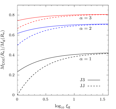
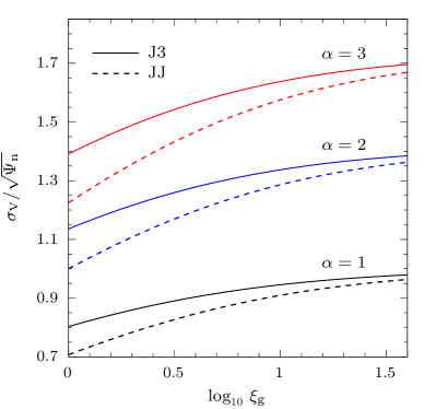
Figure 1: Left: dark-to-total mass ratio of the J3 models (solid lines) within a sphere of radius $r=R_{\rm e}\simeq 0.75\,r_{*}$ as a function of $\xi_{\rm g}=r_{\rm g}/r_{*}$ for the minimum halo case $\alpha=1$ (black), $\alpha=2$ (blue), and $\alpha=3$ (red). For comparison, the analogous curves in the case of JJ models (dashed lines) are shown. Right: the galactic virial velocity dispersion $\sigma_{\rm V}$ (solid lines) as a function of $\xi_{\rm g}$, for $\alpha=1$ (black), $\alpha=2$ (blue), and $\alpha=3$ (red). For comparison, the analogous curves in the case of JJ models (dashed lines) are shown.

The DM halo density profile is therefore

$$\rho_{\rm DM}(r)\equiv\rho_{\rm g}(r)-\rho_{*}(r)=\frac{\rho_{\rm n}}{s^{2}}\left[\hskip 0.85358pt\frac{{\mathcal{R}}_{\rm g}}{\xi_{\rm g}+s}-\frac{1}{(1+s)^{2}}\hskip 0.85358pt\right]\!,$$ (23)

and, as shown in CMP19, the condition for a nowhere negative $\rho_{\rm DM}$ is

$${\mathcal{R}}_{\rm g}\geq{\cal R}_{\rm m}\equiv\begin{cases}\displaystyle{\frac{1}{4\hskip 0.28453pt(1-\xi_{\rm g})}}\hskip 0.56905pt,\hskip 14.22636pt0<\xi_{\rm g}\leq\frac{1}{2}\hskip 0.56905pt,\\[10.0pt] \displaystyle{\hskip 0.7113pt\xi_{\rm g}}\hskip 1.13809pt,\hskip 45.23978pt\xi_{\rm g}\geq\frac{1}{2}.\end{cases}$$ (24)

A model with ${\mathcal{R}}_{\rm g}={\cal R}_{\rm m}$ is called a minimum halo model. For assigned $\xi_{\rm g}$, it is convenient to introduce the parameter $\alpha$, defined as

$${\mathcal{R}}_{\rm g}=\alpha\hskip 0.56905pt{\cal R}_{\rm m}\hskip 1.13809pt,\qquad\quad\alpha\geq 1,$$ (25)

and, as we shall restrict to the natural situation $\xi_{\rm g}\geq 1$, in the following ${\mathcal{R}}_{\rm g}=\alpha\hskip 0.56905pt\xi_{\rm g}$, with $\alpha=1$ corresponding to the minimum halo model. Therefore, from equations (22), the relative amount of dark-to-total mass as a function of radius is

$$\frac{M_{\rm DM}(r)}{M_{\rm g}(r)}=1-\frac{s}{\alpha\hskip 0.56905pt\xi_{\rm g}(1+s)\ln\hskip 0.56905pt(1+s/\xi_{\rm g})}\hskip 0.56905pt,$$ (26)

where $M_{\rm DM}(r)=M_{\rm g}(r)-M_{*}(r)$. In Fig. 1 (left panel, solid lines) we plot equation (26) as a function of $\xi_{\rm g}\geq 1$ for $r=R_{\rm e}$ and for three values of $\alpha$ : the minimum halo model ($\alpha=1$) and two cases with $\alpha>1$. Fractions of DM with values for the minimum halo case in agreement with those required by the dynamical modelling of early-type galaxies (see e.g. Cappellari et al. 2015) can be easily obtained. These fractions are unsurprisingly sligthly larger than those obtained in the case of JJ models for the same values of $\xi_{\rm g}$ (see dashed lines in Fig. 1, left panel).

Notice that by construction, $\rho_{\rm DM}\propto r^{-3}$ at large radii, while, as in JJ models, at small radii $\rho_{\rm DM}\propto r^{-2}$ (i.e. the DM and stellar densities are locally proportional), with the exception of the minimum halo models, in which $\rho_{\rm DM}\propto r^{-1}$. We now compare the DM profile of J3 models with the untruncated NFW profile (Navarro et al. 1997), that in our notation can be written as

$$\rho_{\rm NFW}(r)=\frac{\rho_{\rm n}{\cal R}_{\rm NFW}}{q(c)s\hskip 0.56905pt(\xi_{\rm NFW}+s)^{2}}\hskip 0.56905pt,\quad q(c)\equiv\ln\hskip 0.56905pt(1+c)-\frac{c}{1+c}\hskip 0.56905pt,$$ (27)

where $\xi_{\rm NFW}\equiv r_{\rm NFW}/r_{*}$ is the NFW scale length in units of $r_{*}$ and, for a chosen reference radius $r_{\rm t}$, we define ${\cal R}_{\rm NFW}\equiv M_{\rm NFW}(r_{\rm t})/M_{*}$ and $c\equiv r_{\rm t}/r_{\rm NFW}$. The densities $\rho_{\rm DM}$ and $\rho_{\rm NFW}$ can be made asymptotically identical both at small and large radii by fixing

$${\cal R}_{\rm NFW}=q(c)\hskip 1.13809pt\xi_{\rm g}\hskip 1.13809pt,\qquad\quad\xi_{\rm NFW}=\frac{\xi_{\rm g}}{\sqrt{\hskip 0.85358pt2\hskip 0.85358pt\xi_{\rm g}-1}}\hskip 0.56905pt.$$ (28)

Hence, once a specific minimum halo galaxy model is considered, equations (27) and (28) allow to determine the NFW profile that best reproduces the DM halo density profile. Cosmological simulations suggest for galaxies $c\simeq 10$ (see e.g. Bullock & Boylan-Kolchin 2017), and ${\cal R}_{\rm NFW}\simeq$ a few tens. Moreover, the value of $\xi_{\rm g}$ cannot be too large, otherwise the DM fraction inside $R_{\rm e}$ would exceed the values derived from observations (see e.g. Napolitano et al. 2010; see also Fig. 1 in CMP19). For these reasons we conclude that the NFW shape and the cosmological expectations are reproduced if we consider minimum halo models with $\xi_{\rm g}\simeq 10\div 20$. In the following, we choose as ‘reference model’ a minimum halo model with ${\mathcal{R}}_{\rm g}=\xi_{\rm g}=13$, $c=10$, ${\cal R}_{\rm NFW}\simeq 20$, and $r_{\rm NFW}=2.6\,r_{*}$.

3.1 Central and Virial properties of J3 models

Now we recall a few dynamical properties of the J3 models needed in the following discussion (see CMP19 for more details). A MBH of mass $M_{\rm{BH}}=\mu M_{*}$ is added at the centre of the galaxy, and the total (relative) potential is

$$\Psi_{\rm T}(r)=\frac{\Psi_{\rm n}\mu}{s}+\Psi_{\rm g}(r)\hskip 1.13809pt,\quad\,\,\,\Psi_{\rm n}=\frac{GM_{*}}{r_{*}}\hskip 0.56905pt,\quad\,\,\,\mu=\frac{M_{\rm{BH}}}{M_{*}}\hskip 0.56905pt,$$ (29)

where

$$\Psi_{\rm g}(r)=\frac{\Psi_{\rm n}{\mathcal{R}}_{\rm g}}{\xi_{\rm g}}\left(\hskip 0.7113pt\ln\frac{\xi_{\rm g}+s}{s}+\frac{\xi_{\rm g}}{s}\ln\frac{\xi_{\rm g}+s}{\xi_{\rm g}}\hskip 0.7113pt\right);$$ (30)

in particular, $\Psi_{\rm g}\propto(\ln s)/s$ at large radii, and $\Psi_{\rm g}\propto-\ln s$ near the centre. The stellar orbital structure is limited to the isotropic case. The radial component of the velocity dispersion is given by

$$\sigma_{\rm r}^{2}(r)=\sigma_{\rm BH}^{2}(r)+\sigma_{\rm g}^{2}(r)\hskip 1.13809pt,$$ (31)

where $\sigma_{\rm BH}$ and $\sigma_{\rm g}$ indicate, respectively, the contribution of the MBH and of the galaxy potential. As shown in CMP19, the Jeans equations for J3 models can be solved analytically, here we just recall that in the isotropic case

$$\sigma_{\rm r}^{2}(r)\sim\Psi_{\rm n}\times\begin{cases}\displaystyle\frac{\mu}{3\hskip 0.28453pts}+\frac{{\mathcal{R}}_{\rm g}}{2\hskip 0.56905pt\xi_{\rm g}}-\frac{\mu}{3}\hskip 0.56905pt,\hskip 24.18483ptr\to 0\hskip 0.56905pt,\\[12.0pt] \displaystyle{\mathcal{R}}_{\rm g}\hskip 0.56905pt\frac{\ln s}{5\hskip 0.28453pts}\hskip 0.56905pt,\hskip 50.64586ptr\to\infty\hskip 0.56905pt,\end{cases}$$ (32)

where, for mathematical consistency, we retained also the constant term $-\hskip 0.56905pt\mu/3$ in the asymptotic expansion of $\sigma_{\rm r}$ near the centre, although this contribution is fully negligible in realistic galaxy models. Notice that, when $\xi_{\rm g}\geq 1$, from equation (25) it follows that the constant term due to the galaxy is independent of $\xi_{\rm g}$, with $\sigma_{\rm g}^{2}(0)=\Psi_{\rm n}\alpha/2$. This latter expression provides the interesting possibility of adopting $\sigma_{\rm g}(0)$ as a proxy for the observed velocity dispersion of the galaxy in the central regions, outside the sphere of influence of the central MBH.

In order to derive an estimate of the sphere of influence of the MBH, it is interesting to consider the projected velocity dispersion $\sigma_{\rm p}(R\hskip 0.85358pt)=\sqrt{\hskip 0.85358pt\sigma_{\rm pBH}^{2}(R\hskip 0.85358pt)+\sigma_{\rm pg}^{2}(R\hskip 0.85358pt)\hskip 0.56905pt}\hskip 0.56905pt$, where $R$ is the radius in the projection plane. At large radii $\sigma_{\rm p}$ is dominated by the galaxy contribution: from equation (32) one has, at the leading order,

$$\sigma_{\rm p}^{2}(R\hskip 0.85358pt)\sim\frac{\Psi_{\rm n}\hskip 0.42677pt8\hskip 0.56905pt{\mathcal{R}}_{\rm g}\ln\eta}{15\pi\eta}\hskip 0.56905pt,\qquad\eta\equiv\frac{R}{r_{*}}.$$ (33)

At small radii, instead (CMP19, equations (57) and (58)),

$$\sigma_{\rm pg}(0)=\sigma_{\rm g}(0)=\frac{\Psi_{\rm n}{\mathcal{R}}_{\rm g}}{2\hskip 0.56905pt\xi_{\rm g}}\hskip 0.56905pt,\qquad\,\,\,\,\,\sigma_{\rm pBH}^{2}(R\hskip 0.85358pt)\sim\frac{\Psi_{\rm n}\hskip 0.42677pt2\hskip 0.56905pt\mu}{3\pi\eta}\hskip 0.28453pt.$$ (34)

Equation (34) allows to estimate the radius $R_{\rm inf}$ of the sphere of influence, defined as the distance from the centre in the projection plane where $\sigma_{\rm p}$ in presence of the MBH exceedes by a factor $(1+\epsilon)$ the galaxy projected velocity dispersion $\sigma_{\rm pg}$ in absence of the MBH:

$$\sqrt{\hskip 1.13809pt\sigma_{\rm pBH}^{2}(R_{\rm inf})+\sigma_{\rm pg}^{2}(R_{\rm inf})\hskip 1.13809pt}\hskip 1.42262pt\equiv\hskip 0.56905pt(1+\epsilon)\hskip 0.56905pt\sigma_{\rm pg}(R_{\rm inf})\hskip 0.85358pt.$$ (35)

In practice, for a galaxy model with finite $\sigma_{\rm pg}(0)$, the formula above reduces to equation (36) in CP18, and for $\xi_{\rm g}\geq 1$ equation (34) yields

$$\frac{R_{\rm inf}}{r_{*}}\simeq\frac{4\mu}{3\pi\alpha\hskip 0.56905pt\epsilon\hskip 0.56905pt(2+\epsilon)}\hskip 0.56905pt.$$ (36)

Notice that equation (36) is coincident with the same estimate in JJ models (CP18, equation 37), being the two models identical in the central regions.

A fundamental ingredient in Bondi accretion is the gas temperature at infinity $T_{\infty}$. As in CP18, in the next Section we shall use $T_{\rm V}\!=\!\langle\mu\rangle\hskip 0.28453ptm_{\rm p}\hskip 0.56905pt\sigma_{\rm V}^{2}/(3\hskip 0.56905ptk_{\rm B})$ (see e.g. Pellegrini 2011) as the natural scale for $T_{\infty}$, where $\sigma_{\rm V}$ is the (three dimensional) virial velocity dispersion of stars obtained from the Virial Theorem:

$$M_{*}\sigma_{\rm V}^{2}\equiv 2K_{*}=-\hskip 1.99168ptW_{\rm*g}-W_{\rm*BH}\hskip 0.56905pt.$$ (37)

In the equation above, $K_{*}$ is the total kinetic energy of the stars,

$$W_{\rm*g}=-\,4\pi G\!\int_{0}^{\infty}\!M_{\rm g}(r)\rho_{*}(r)\hskip 0.85358ptrdr$$ (38)

is the interaction energy of the stars with the gravitational field of the galaxy (stars plus DM), and the MBH contribution $W_{\rm*BH}$ diverges near the origin for a Jaffe density distribution. Since we shall use $\sigma_{\rm V}$ as a proxy for the gas temperature at large distance from the centre, we neglect $W_{\rm*BH}$ in equation (37), so that

$$\sigma_{\rm V}^{2}=-\hskip 1.13809pt\frac{W_{\rm*g}}{M_{*}}=\Psi_{\rm n}{\mathcal{R}}_{\rm g}\widetilde{W}_{\rm*g}\hskip 0.56905pt,\qquad\widetilde{W}_{\rm*g}={\cal H}(\xi_{\rm g},0)-\frac{\ln\xi_{\rm g}}{\xi_{\rm g}-1}\hskip 0.56905pt,$$ (39)

where the function ${\cal H}(\xi_{\rm g},s)$ is given in Appendix C of CMP19. Fig. 1 (right panel) shows the trend of $\sigma_{\rm V}$ as a function of $\xi_{\rm g}\geq 1$, for three J3 (solid) and JJ (dashed) models. As expected, $\sigma_{\rm V}$ increases with $\xi_{\rm g}$, and $\sigma_{\rm V}\simeq\sqrt{\alpha\hskip 0.28453pt\Psi_{\rm n}}$ when $r_{\rm g}\gg r_{*}$. For comparison, we show in Fig. 1 (right panel) $\sigma_{\rm V}$ for the JJ models of same parameters.

Table 2: Galaxy Structure and Accretion Flow parameters

Galaxy Structure		Accretion Flow
Symbol	Quantity	Symbol	Quantity
$M_{*}$	Total stellar mass	$T_{\infty}$	Gas temperature at infinity
$r_{*}$	Stellar density scale length	$\rho_{\infty}$	Gas density at infinity
$M_{\rm g}$	Total${}^{\hskip 0.7113pt\rm a}$a galaxy mass	$c_{\infty}$	Speed of sound at infinity
$r_{\rm g}$	Total density scale length	$\gamma$	Polytropic index ($1\leq\gamma\leq 5/3$)
$M_{\rm{BH}}$	Central MBH mass	$\gamma_{\rm ad}$	Adiabatic index ($\hskip 0.42677pt={\cal C}_{p}/{\cal C}_{V}$)
$\mu$	$M_{\rm{BH}}/M_{*}$	${\cal R}$	$M_{\rm g}/M_{\rm{BH}}$ ($\hskip 0.42677pt={\mathcal{R}}_{\rm g}/\mu$)
${\mathcal{R}}_{\rm g}$	$M_{\rm g}/M_{*}$ ($\hskip 0.42677pt=\alpha\hskip 0.28453pt{\cal R}_{\rm m}\hskip 0.56905pt$)	$\beta$	$T_{\infty}/T_{\rm V}$
${\cal R}_{\rm m}$	Minimum value of ${\mathcal{R}}_{\rm g}$	$r_{\rm B}$	Bondi radius
$\xi_{\rm g}$	$r_{\rm g}/r_{*}$	$r_{\rm min}$	Sonic radius
$s$	$r/r_{*}$	$x$	$r/r_{\rm B}$
$\sigma_{\rm V}$	Stellar virial velocity dispersion	$\xi$	$r_{\rm g}/r_{\rm B}$
$T_{\rm V}$	Stellar virial temperature	$\lambdaup_{\hskip 0.56905pt{\rm t}}$	Critical accretion parameter
$W_{\rm*g}$	Virial energy of stars	$\mathcal{M}$	Mach number

• For example, from our definition $M_{\rm g}={\mathcal{R}}_{\rm g}M_{*}$, and equation (20), $M_{\rm g}$ is the total mass (stellar plus DM) inside a sphere of radius $({\rm e}-1)\hskip 0.85358ptr_{\rm g}$.

3.2 Linking Stellar Dynamics to Fluid Dynamics

We now link the stellar dynamical properties of the galaxy models with the defining parameters of Bondi accretion introduced in Section 2.2. In fact, the function $f$ in equation (19) is written in terms of quantities referring to the central MBH and to the gas temperature at infinity, while the stellar dynamical properties of the J3 models are written in terms of the observational properties of the galaxy stellar component. The two groups of parameters are summarised in Table 2.

The first accretion parameter we consider is ${\cal R}$ in equation (17). It is linked to the galaxy structure by the following expression

$${\cal R}\equiv\frac{M_{\rm g}}{M_{\rm{BH}}}=\frac{{\mathcal{R}}_{\rm g}}{\mu}=\frac{\alpha\hskip 0.85358pt\xi_{\rm g}}{\mu}\hskip 0.56905pt,$$ (40)

where the last identity derives from equation (25) with $\xi_{\rm g}\geq 1$; notice that ${\cal R}\approx 10^{4}$ for $\xi_{\rm g}$ of the order of tens and $\alpha$ of order unity, and $\mu=0.002$ (see Kormendy & Ho 2013 for this choice of $\mu$).

The determination of the accretion parameter $\xi$ is more articulated. This quantity depends on the Bondi radius $r_{\rm B}$; we stress again that in the present discussion, even in presence of the galaxy gravitational potential, $r_{\rm B}$ is still defined in the classical sense, i.e., just considering the mass of the MBH, as in equation (4). Of course, $r_{\rm B}$ depends on the gas temperature at infinity. In principle, arbitrary values of $T_{\infty}$ could be adopted, but in real systems the natural scale for the global temperature is represented by the virial temperature $T_{\rm V}$ defined via the virial velocity dispersion in equation (37). Accordingly, we set

$$T_{\infty}=\beta\hskip 0.85358ptT_{\rm V},\qquad c_{\infty}^{2}=\gamma\hskip 1.13809pt\frac{p_{\infty}}{\rho_{\infty}}=\frac{\gamma\beta\hskip 0.28453pt\sigma_{\rm V}^{2}}{3}.$$ (41)

From equations (4) and (39) we then obtain

$$\frac{r_{\rm B}}{r_{*}}=\frac{3\mu}{\alpha\beta\gamma\hskip 0.28453pt{\cal F}_{\rm g}(\xi_{\rm g})}\hskip 0.85358pt,\qquad\quad{\cal F}_{\rm g}\equiv\xi_{\rm g}\hskip 0.56905pt\widetilde{W}_{\rm*g}(\xi_{\rm g})\hskip 0.85358pt,$$ (42)

where the function ${\cal F}_{\rm g}$ monothonically increases with $\xi_{\rm g}$ from ${\cal F}_{\rm g}(1)=\pi^{2}/\hskip 0.42677pt6-1$ to ${\cal F}_{\rm g}(\infty)=1$. For example, at fixed $\alpha$, $\beta$, and $\gamma$, one has

$$\frac{3\mu}{\alpha\beta\gamma}<\frac{r_{\rm B}}{r_{*}}\leq\frac{18\mu}{(\pi^{2}-6)\hskip 0.28453pt\alpha\beta\gamma}.$$ (43)

In Fig. 2 (top left) we show the trend of $r_{\rm B}/r_{*}$ as a function of $\xi_{\rm g}$ in the minimum halo case ($\alpha=1$) with $\beta=1$ and $\mu=0.002$, for three values of $\gamma$; in general, $r_{\rm B}$ is of the order of a few $\times\hskip 1.42262pt10^{-3}\hskip 0.85358ptr_{*}$. Note that, for fixed $\xi_{\rm g}$, the isothermal profile (black line) is above that in the corresponding adiabatic case (red line); in general, for fixed $\alpha$, $\beta$ and $\xi_{\rm g}$, $r_{\rm B}/r_{*}$ always lies between the isothermal and the monoatomic adiabatic case, as shown by equation (43). Finally, by combining equations (17) and (42),

$$\xi\equiv\frac{r_{\rm g}}{r_{\rm B}}=\frac{\alpha\beta\gamma\hskip 0.56905pt\xi_{\rm g}{\cal F}_{\rm g}(\xi_{\rm g})}{3\mu}=\frac{{\cal R}\beta\hskip 0.56905pt\gamma{\cal F}_{\rm g}(\xi_{\rm g})}{3}\hskip 0.56905pt,$$ (44)

and so ${\cal R}$ and $\xi$ increase with $\xi_{\rm g}$. Curiously, from the general definitions in equation (17), and making use of equation (34),

$$\frac{{\cal R}}{\xi}=\frac{2\hskip 0.85358pt\sigma_{\rm pg}^{2}(0)}{c_{\infty}^{2}},$$ (45)

which links directly the parameters of Bondi accretion to the observable $\sigma_{\rm pg}(0)=\sigma_{\rm g}(0)$.

For observational purposes, it is also useful to express the position of $r_{\rm B}$ in terms of the radius $R_{\rm inf}$ as given in equation (36); since the parameter $\alpha={\mathcal{R}}_{\rm g}/{\cal R}_{\rm m}$ cancels out, we have

$$\frac{r_{\rm B}}{R_{\rm inf}}=\frac{9\pi\hskip 0.28453pt\epsilon\hskip 0.56905pt(2+\epsilon)}{4\hskip 0.28453pt\beta\gamma{\cal F}_{\rm g}(\xi_{\rm g})}\hskip 0.56905pt,$$ (46)

independently of the minimum halo assumption. In Fig. 2 (bottom left panel) we show the trend of $r_{\rm B}/R_{\rm inf}$ when $\epsilon=0.5$ and $\beta=1$, for the same three values of $\gamma$ as in the upper left panel: $r_{\rm B}\approx$ a few times $R_{\rm inf}$.

Now we move the discussion to the sonic radius $r_{\rm min}$, one of the most important properties of the accretion solution. The effects of the galaxy do indeed manifest themselves in the position of $r_{\rm min}$. When measured in terms of the scale length $r_{*}$, it can be written, by making use of equation (42), as

$$\frac{r_{\rm min}}{r_{*}}=\hskip 1.70717ptx_{\rm min}(\chiup,{\cal R},\xi)\hskip 1.13809pt\frac{r_{\rm B}}{r_{*}}\hskip 0.56905pt,$$ (47)

where $x_{\rm min}\equiv r_{\rm min}/r_{\rm B}$ gives the (absolute) minimum of $f$.

Finally, we must recast the galaxy potential in equation (30) by using the normalization scales in equation (18) : as $s/\xi_{\rm g}=x/\xi$, it is immediate that in our problem

$$\psi\!\left(\frac{x}{\xi}\right)\!=\ln\!\left(1+\frac{\xi}{x}\right)+\hskip 0.7113pt\frac{\xi}{x}\ln\!\left(1+\frac{x}{\xi}\right).$$ (48)

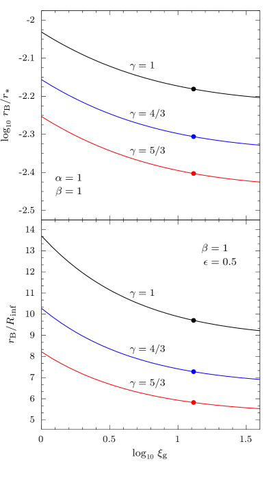
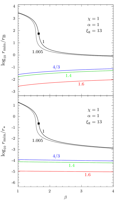
Figure 2: Left: Bondi radius $r_{\rm B}$ in units of $r_{*}$ (top) and $R_{\rm inf}$ (bottom), as a function of the galaxy-to-stellar scale length ratio $\xi_{\rm g}=r_{\rm g}/r_{*}$, for three J3 galaxy models with $\beta\equiv T_{\rm V}/T_{\infty}=1$, $\mu=0.002$, and $\gamma=1$, $4/3$, $5/3$; the solid dots at $r_{\rm B}/r_{*}\simeq 0.0066$, $0.0049$, $0.0039$ correspond to the minimum halo case with $\xi_{\rm g}=13$; solid dots at $r_{\rm B}/R_{\rm inf}\simeq 9.71$, $7.28$, $5.82$ correspond to the case $\xi_{\rm g}=13$ and $\epsilon=0.5$. Right: position of $x_{\rm min}\equiv r_{\rm min}/r_{\rm B}$ (top) and $r_{\rm min}/r_{*}$ (bottom) as a function of $\beta=T_{\infty}/T_{\rm V}$, in the case of minimum halo models with $\xi_{\rm g}=13$, $\mu=0.002$, and $\chiup=1$, for different values of the polytropic index given close to the curves. The black square points at $r_{\rm min}/r_{\rm B}\simeq 57.34$ and $r_{\rm min}/r_{*}\simeq 0.23$ correspond to the critical case $\beta=\beta_{\rm c}\simeq 1.65$.

4 Bondi accretion in J3 models

We can now discuss the full problem, investigating how the standard Bondi accretion is modified by the additional potential of J3 galaxies, and by electron scattering. We show that in the isothermal case ($\gamma=1$) the solution is fully analytical, as for the monoatomic adiabatic case ($\gamma=5/3$); for $1<\gamma<5/3$, instead, it is not possible to obtain analytical expressions, and so a numerical investigation is presented.

4.1 The $\gamma=1$ case

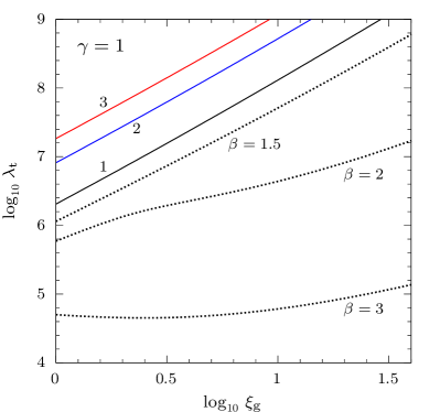
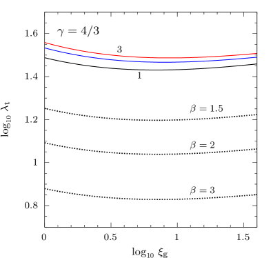
Figure 3: Critical accretion parameter $\lambdaup_{\hskip 0.56905pt{\rm t}}$ as a function of $\xi_{\rm g}$, for the minimum halo case $\alpha=1$ (black), $2$ (blue), and $3$ (red), and $\chiup=1$ and $\beta=1$. The dotted curves refer to $\alpha=1$ and three different values of $\beta$. The left panel shows the case $\gamma=1$, the right panel shows the case $\gamma=4/3$. Notice that $\lambdaup_{\hskip 0.56905pt{\rm t}}$ in the isothermal case is several order of magnitude larger than the $\gamma=4/3$ case.

The isothermal case stands out not only because $f(x)$ in equation (19) is not of the general family, for $\gamma=1$, but also because the position of the sonic radius $x_{\rm min}$ can be obtained explicitely. Indeed, for $0<\chiup\leq 1$, $f(x)\sim\chiup/x$ for $x\to 0$, and $\sim 2\ln x$ for $x\to\infty$. Therefore, the continuous function $f$ has at least one critical point over the range $0\leq x<\infty$, obtained by solving

$$2\hskip 0.56905ptx_{\rm min}-{\cal R}\ln\frac{\xi+x_{\rm min}}{\xi}=\chiup\hskip 0.85358pt.$$ (49)

As shown in Appendix A, the positive solution can be obtained for generic values of the model parameters in terms of the Lambert-Euler $W$ function, and the only minimum of $f$ is reached at

$$x_{\rm min}\equiv\frac{r_{\rm min}}{r_{\rm B}}=-\hskip 2.27621pt\xi-\frac{{\cal R}}{2}\,W_{-1}\left(-\hskip 1.42262pt\frac{2\xi}{{\cal R}}\hskip 1.13809pt{\rm e}^{-\hskip 1.13809pt\frac{\chiup+2\xi}{{\cal R}}}\right).$$ (50)

Once $x_{\rm min}$ is known, all the other quantities in the Bondi solution, such as the critical accretion parameter $\lambdaup_{\hskip 0.56905pt{\rm t}}=\exp\hskip 0.7113pt(f_{\rm min}-1/2)$ in equation (14), the mass accretion rate in equation (2), and the Mach number profile $\mathcal{M}$, can be expressed as a function of $x_{\rm min}$. Therefore, J3 galaxies belong to the family of models for which a fully analytical discussion of the isothermal Bondi accretion problem is possible (see Table 1). In particular, from CP17 and CP18, the critical accretion solution reads

$$\mathcal{M}^{2}=-\begin{cases}\displaystyle{W_{0}\hskip 0.56905pt\big{(}-\lambdaup_{\hskip 0.56905pt{\rm t}}^{2}\hskip 0.85358pt{\rm e}^{-2f}\big{)}}\hskip 0.85358pt,\hskip 31.29802ptx\geq x_{\rm min}\hskip 0.85358pt,\\[7.0pt] \displaystyle{W_{-1}\hskip 0.56905pt\big{(}-\lambdaup_{\hskip 0.56905pt{\rm t}}^{2}\hskip 0.85358pt{\rm e}^{-2f}\big{)}}\hskip 0.85358pt,\hskip 18.49428pt0<x\leq x_{\rm min}\hskip 0.85358pt,\end{cases}$$ (51)

where $f$ is given in equation (19) with the function $\psi(x/\xi)$ defined by equation (48). Summarising, $W_{-1}$ describes supersonic accretion, while $W_{0}$ subsonic accretion. Although equation (51) provides an explicit expression of $\mathcal{M}$, it can be useful to have its asymptotic trend at small and large distances from the centre; from equation (77) and the expansion of $f(x)$, one has

$$\mathcal{M}^{2}\sim\begin{cases}\displaystyle{\frac{2\chiup}{x}+\frac{2(2\xi-{\cal R})}{\xi}\ln\frac{x}{x_{\rm min}}}\hskip 0.56905pt,\hskip 22.76228ptx\to 0\hskip 1.13809pt,\\[12.0pt] \displaystyle{\lambdaup_{\hskip 0.56905pt{\rm t}}^{2}\hskip 1.13809ptx^{-\hskip 0.7113pt2\hskip 0.28453pt\left(2\hskip 1.13809pt+\frac{{\cal R}}{x}\right)}}\hskip 0.56905pt,\hskip 64.67296ptx\to\infty\hskip 0.28453pt.\end{cases}$$ (52)

Of course, the same result can be established also by asympotic expansion of equation (12). Therefore, in the central region $\mathcal{M}\propto x^{-1/2}$ for $\chiup>0$, while $\mathcal{M}\sim\sqrt{\hskip 0.56905pt2(2-{\cal R}/\xi)\ln\hskip 0.56905pt(x/x_{\rm min})}$ when $\chiup=0$ (provided that ${\cal R}>2\xi$).

As already found for JJ models in the isothermal case, also for J3 models the case $\chiup=0$ (from equation (18) corresponding to a galaxy without a central MBH) reveals some interesting properties of the gas flow, also relevant for the understanding of the more natural situation $\chiup>0$. In fact, near the centre $f(x)\sim(2-{\cal R}/\xi)\ln x$, and a solution is possible only for ${\cal R}\geq 2\xi$, with $x_{\rm min}$ given by equation (50). When ${\cal R}<2\xi$, $f_{\rm min}=-\,\infty$ (reached at the origin), and therefore no accretion is possible since $\lambdaup_{\hskip 0.56905pt{\rm t}}$ would be zero. In the special case $\chiup=0$ and ${\cal R}=2\xi$, $f_{\rm min}$ is again reached at the origin, but $f$ now converges to $f_{\rm min}=2(1+\ln\xi)$, with $\lambdaup_{\hskip 0.56905pt{\rm t}}=\xi^{2}{\rm e}^{3/2}$. Given the similarity of JJ and J3 models near the centre, the fact that both models share the same properties at small radii is not surprising. Equation (52) can still be used with $\chiup=0$ for ${\cal R}>2\xi$, while for ${\cal R}=2\xi$, from equations (51) and (77) it can be shown that $\mathcal{M}^{2}=1+{\cal O}(x)$.

We now show how the condition ${\cal R}\geq 2\xi$ when $\chiup=0$, in order to have accretion, imposes an upper limit on $T_{\infty}$. In fact, from equation (44), with $\gamma=1$, the identity ${\cal R}/(2\xi)=3/(2\beta{\cal F}_{\rm g})$ produces a condition for $\beta$ :

$$\beta\leq\frac{3}{2{\cal F}_{\rm g}(\xi_{\rm g})}\equiv\beta_{\rm c}\hskip 0.56905pt,$$ (53)

where the critical parameter $\beta_{\rm c}$ depends only on $\xi_{\rm g}$. It follows that in absence of a central MBH, isothermal accretion in J3 galaxies is possible only for

$$T_{\infty}\leq\beta_{\rm c}\hskip 0.85358ptT_{\rm V}\hskip 0.56905pt,\quad\,{\rm i.e.},\quad\,\sigma_{\rm pg}(0)=\sigma_{\rm g}(0)\geq c_{\infty}\hskip 1.13809pt,$$ (54)

where the last inequality derives from equation (45). For reference, in Fig. 4 (right panel) we show $\beta_{\rm c}$ as a function of $\xi_{\rm g}$, for both JJ and J3 models; it is easy to prove that $3/2<\beta_{\rm c}\leq 9/(\pi^{2}\!-6)\simeq 2.33$.

As anticipated, the limitation ${\cal R}\geq 2\xi$ when $\chiup=0$ is also relevant for the understanding of the flow behaviour when $\chiup>0$. In fact, it is possible to show that, by defining $\tau\equiv\beta/\beta_{\rm c}=2\xi/{\cal R}$, for ${\cal R}\to\infty$ and fixed $\tau$, we have

$$x_{\rm min}\sim\begin{cases}\displaystyle-\hskip 1.13809pt\frac{\tau+W_{-1}(-\hskip 1.13809pt\tau\hskip 0.56905pt{\rm e}^{-\hskip 0.56905pt\tau})}{2}\hskip 1.13809pt{\cal R}\hskip 1.13809pt,\hskip 21.33955pt\tau<1\hskip 0.56905pt,\\[10.0pt] \displaystyle\sqrt{\frac{\chiup\hskip 0.56905pt{\cal R}}{2}}\hskip 1.13809pt,\hskip 78.38747pt\tau=1\hskip 0.56905pt,\\[14.0pt] \displaystyle\frac{\chiup\hskip 0.56905pt\tau}{2\hskip 0.56905pt(\tau-1)}\hskip 1.13809pt,\hskip 69.70915pt\tau>1.\end{cases}$$ (55)

The trend of $x_{\rm min}$ as a function of $\beta$ is shown by the black solid line in Fig. 2 (top right panel), for a minimum halo model with $\xi_{\rm g}=13$ and $\mu=0.002$. For example, equation (55) allows to explain the drop at increasing $\beta$ when $\tau$ switches from being less than unity to being larger than unity, with $x_{\rm min}\simeq\chiup/2$ independently of $\tau$; the black square point at $r_{\rm min}\simeq 57.34\,r_{\rm B}$ correspond to $\beta=\beta_{\rm c}\simeq 1.65$, well approximated by the value $57.01\,r_{\rm B}$ obtained with the previous equation. Equation (55) allows us to find the behaviour of $\lambdaup_{\hskip 0.56905pt{\rm t}}$ for large values of ${\cal R}$ (at fixed $\beta$). For example, in the peculiar case $\beta=\beta_{\rm c}$ (i.e. $\tau=1$), an asymptotic analysis shows that $\lambdaup_{\hskip 0.56905pt{\rm t}}\sim{\rm e}^{3/2}{\cal R}^{2}/4$; for simplicity, we do not report the expression of $\lambdaup_{\hskip 0.56905pt{\rm t}}$ for $\beta\neq\beta_{\rm c}$, which can, however, be easily calculated. As shown in Fig. 3 (left panel), the presence of the galaxy makes $\lambdaup_{\hskip 0.56905pt{\rm t}}$ several orders of magnitude larger than without it.

A summary of the results can be seen by inspection of Fig. 5 (top panels), where we show the radial profile of the Mach number for three different values of the temperature parameter ($\beta=1$, $2$, $3$). Solid lines show the two critical solutions, one in which the gas flow begins supersonic and approaches the centre with zero velocity, and the other in which $\mathcal{M}$ continuously increases towards the centre. The dotted lines show two illustrative subcritical solutions with $\lambdaup=0.8\,\lambdaup_{\hskip 0.56905pt{\rm t}}$. It is apparent that $r_{\rm min}$ decreases very rapidly with increasing temperature at the transition from $\beta=1$ to $\beta=2$: $r_{\rm min}\simeq 19.89\,r_{*}$, $0.0093\,r_{*}$, and $0.0024\,r_{*}$, for $\beta=1$, $2$, and $3$, respectively.

Finally, once the Mach number profile is known, the gas density profile is obtained from the first equation of the system (6) with $\gamma=1$, i.e.,

$$\tilde{\rho}(x)=\frac{\rho(x)}{\rho_{\infty}}=\frac{\lambdaup}{x^{2}\mathcal{M}(x)}.$$ (56)

Along the critical solution, by virtue of equation (52) it follows that $\tilde{\rho}\sim\lambdaup_{\hskip 0.56905pt{\rm t}}\hskip 0.56905ptx^{-\hskip 0.56905pt3/2}/\sqrt{2\chiup}$ at the centre when $\chiup>0$, while $\tilde{\rho}\sim x^{{\cal R}/x}$ at large radii. Fig. 6 (top panel) shows the radial trend of $\tilde{\rho}$ for the critical accretion solution in our reference model, with $\lambdaup_{\hskip 0.56905pt{\rm t}}\simeq 2.14\times 10^{8}$. The bottom panel shows the gas velocity profile and, for comparision, the isotropic velocity dispersion $\sigma_{\rm r}$. Notice that near the centre, $\sigma_{\rm BH}\propto r^{-\hskip 0.56905pt1/2}$ and $\varv=c_{\infty}\hskip 0.85358pt\mathcal{M}\propto r^{-\hskip 0.56905pt1/2}$ (provided that $\chiup>0$), so that their ratio is constant; it can be easily shown that $\varv/\sigma_{\rm BH}\sim 6\hskip 0.56905pt\chiup$. The value of $\sigma_{\rm BH}$ near the centre (i.e. of $\sigma_{\rm r}$ if a central MBH is present), is then a proxy for the isothermal gas inflow velocity.

Figure 4: Critical temperature parameter $\beta_{\rm c}\equiv 3/[\hskip 0.42677pt2\hskip 0.56905pt{\cal F}_{\rm g}(\xi_{\rm g})]$ as a function of $\xi_{\rm g}$, for J3 and JJ galaxy models. For $\beta=T_{\infty}/T_{\rm V}>1$, the isothermal accretion in absence of a central MBH is possible provided that $\beta\leq\beta_{\rm c}$. In these circumstances, once $\xi_{\rm g}$ is fixed, the upper limit of $\beta$ for J3 models is lower than that for JJ ones.

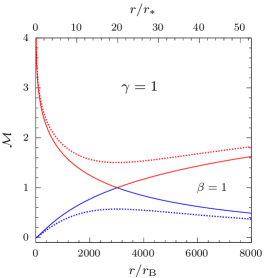
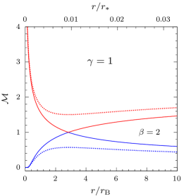
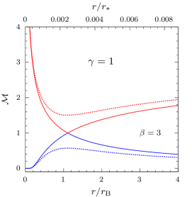
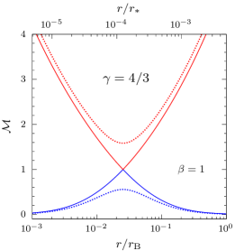
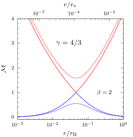
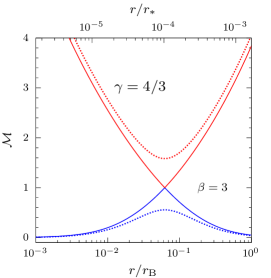
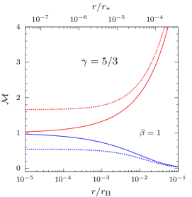
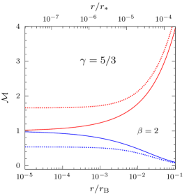
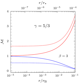
Figure 5: Radial profile of the Mach number for polytropic Bondi problem in a minimum halo J3 galaxy model with $\xi_{\rm g}=13$, $\chiup=1$ and $\mu=0.002$, in case of three different values of the gas temperature ($\beta=1$, $2$, $3$). Solid lines show the two critical solutions ($\lambdaup=\lambdaup_{\hskip 0.56905pt{\rm t}}$), while dotted lines indicate the two subcritical solutions ($\lambdaup=0.8\,\lambdaup_{\hskip 0.56905pt{\rm t}}$); the distance from the centre is given in units of both $r_{\rm B}$ (bottom axis) and $r_{*}$ (top axis, using equation (42)). In blue we plot the subsonic regime and in red the supersonic one. The top panels show the isothermal case ($\gamma=1$): notice how, in accordance with Fig. 2, the position of $r_{\rm min}$ decreases very rapidly passing from $\beta=1$ to $\beta=2$. Middle panels show the case $\gamma=4/3$: in accordance with the dashed black lines in Fig. 2, $r_{\rm min}/r_{*}$ decreases for increasing $\beta$, while $r_{\rm min}/r_{*}$ decreases (note that a logarithmic scale for radius axes has been used). Finally, bottom panels show the adiabatic case ($\gamma=5/3$): the position of the sonic point is reached at the centre, the accretion solutions are always subsonic (i.e. $\mathcal{M}<1$), and the wind solutions are always supersonic (i.e. $\mathcal{M}>1$).

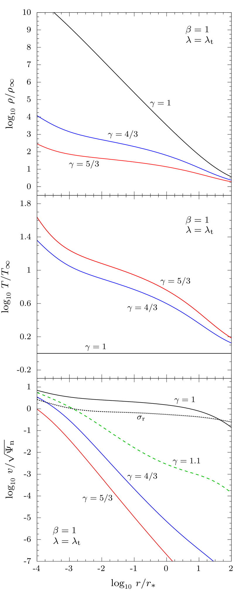
Figure 6: Density (top), temperature (middle), and velocity (bottom) profiles, as a function of $r/r_{*}$, for the critical (i.e. $\lambdaup=\lambdaup_{\hskip 0.56905pt{\rm t}}$) accretion solution of the polytropic Bondi problem in a minimum halo J3 galaxy model with $\xi_{\rm g}=13$, $\chiup=1$, and $\mu=0.002$. The gas temperature at infinity $T_{\infty}$ equals the stellar virial temperature $T_{\rm V}$, i.e. $\beta=1$. For comparison, the dotted line in the bottom panel shows the isotropic velocity dispersion profile $\sigma_{\rm r}$.

4.2 The $1<\gamma<5/3$ case

When $1<\gamma<5/3$, from the expression for $f(x)$ we have that in one case the determination of $x_{\rm min}$ and $f_{\rm min}$ is trivial, i.e. for $\xi\to\infty$ (or ${\cal R}\to 0$) : in this situation the galaxy contribution vanishes, and the position of the only minimum of $f$ reduces to $x_{\rm min}=\chiup\hskip 0.56905pt(5-3\gamma)/4$. Therefore, following KCP16, the behaviour of the associated $\lambdaup_{\hskip 0.56905pt{\rm t}}$ could be found just by carrying out a perturbative analysis (see KCP16, Appendix A); however, since in our models ${\cal R}$ falls in the range $10^{3}\div 10^{4}$, we shall not further discuss this limit case. In general, the problem of the determination of $x_{\rm min}$ (and so of $\lambdaup_{\hskip 0.56905pt{\rm t}}$) cannot be solved analytically, as apparent by combining equations (19) and (48), and setting $df/dx=0$ ; a numerical investigation is then needed. As in the case of isothermal flows, we begin by considering $0<\chiup\leq 1$. Of course, as $f$ is strictly positive, continuous, and divergent to infinity for $x\to 0$ and $x\to\infty$, the existence of at least a minimum is guaranteed. A detailed numerical exploration shows that, in analogy with the isothermal case in Hernquist galaxies (CP17), it is possible to have more than one critical point for $f$ as a function of $\beta$ an $\gamma$. In particular, there can be a single minimum for $f$, or two minima and one maximum. We found that for $\xi_{\rm g}=13$ and $\beta\approx 1\div 2$, only one minimum is present for $\gamma\lesssim 1.01$ and $\gamma\gtrsim 1.1$; instead, for $1.01\lesssim\gamma\lesssim 1.1$, three critical points and two minima are present. When $\beta$ is small (i.e. $T_{\infty}$ is low), the absolute minimum of $f$ is reached at the outer critical point; as $\beta$ increases, the value of $f$ at the inner critical point decreases, and the flow is finally characterised by two sonic points. Increasing further $T_{\infty}$, the inner critical point becomes the new sonic point, with a jump to a smaller value. Fig. 2 (top right panel) shows the position of $x_{\rm min}$ as a function of $\beta$ for different values of $\gamma$, and confirms these trends of $x_{\rm min}$ with $T_{\infty}$ and $\gamma$. Notice how the location of $x_{\rm min}$ (shown in the bottom panel) now decreases with an extremely slow decline for $\gamma>1$. According with equation (47), this means that, for polytropic indeces sufficiently greater than $1$, the ratio $r_{\rm B}/r_{*}$ decreases faster than what $x_{\rm min}$ increases.

In the case $\chiup=0$ the sonic point is reached at the origin. Indeed, $f$ tends to zero when $x\to 0$, and runs to infinity for $x\to\infty$, and so $x_{\rm min}\to 0$ for every choice of the model parameters. Therefore, from equation (11) one has $\lambdaup_{\hskip 0.56905pt{\rm t}}\to 0$, concluding the discussion of the problem in absence of the central MBH since no accretion can take place.

Having determined the position $x_{\rm min}$, we can compute numerically the corresponding value of $\lambdaup_{\hskip 0.56905pt{\rm t}}$, given in the polytropic case by equation (11) with $f_{\rm min}=f(x_{\rm min})$ obtained from equation (19). In Fig. 3 (right panel) the critical accretion parameter is shown as a function of $\xi_{\rm g}$, for a reference model with $\gamma=4/3$ and different values of $\beta$. We note that, at variance with the isothermal case (left panel), $\lambdaup_{\hskip 0.56905pt{\rm t}}$ is roughly constant for fixed $\beta$ independently of the extension of the DM halo, while, at fixed $\xi_{\rm g}$, it increases for decreasing $T_{\infty}$. Having also determined $\lambdaup_{\hskip 0.56905pt{\rm t}}$, we finally solve numerically equation (8), obtaining the Mach profile $\mathcal{M}(x)$. In Fig. 5 (middle panels) we show $\mathcal{M}(x)$ for three different values of the temperature parameter ($\beta=1$, $2$, $3$). The logarithmic scale allows to appreciate how, according to Fig. 2, $x_{\rm min}$ suddenly falls down to values under unity as $\gamma$ increases with respect to the isothermal case. As an illustrative example, we show the case $\gamma=4/3$. Although the trend is not very strong, the location of the sonic point, at variance with the $\gamma=1$ case, moves away from the centre as the temperature increases: $r_{\rm min}\simeq 0.025\,r_{\rm B}$, $0.046\,r_{\rm B}$, and $0.062\,r_{\rm B}$, for $\beta=1$, $2$, and $3$, respectively. For comparison, in the top axis we give the distance from the origin in units of $r_{*}$, from which it can be seen that, in accordance with Fig. 2 (bottom panel), $r_{\rm min}$ now tends to increase slightly, while still of the order of $10^{-4}\,r_{*}$.

Once the radial profile of the Mach number is known, both the gas density and temperature profiles can be obtained from the following relations:

$$\tilde{\rho}\hskip 0.7113pt=\hskip 0.85358pt\tilde{T}^{\hskip 0.99585pt\frac{1}{\gamma-1}}=\hskip 0.85358pt\left(\frac{\lambdaup}{x^{2}\mathcal{M}}\right)^{\frac{2}{\gamma+1}},$$ (57)

with $\tilde{T}=T/T_{\infty}$. Fig. 6 shows the trends of $\rho$ (top panel) and $T$ (middle panel), as a function of $r/r_{*}$, for the critical accretion solution in our usual reference model. The parameter $\beta$ is fixed to unity, and the curves refer to different polytropic indeces.

For what concerns the Mach profile for the critical accretion solution, an asymptotic analysis of equation (8) shows that, at the leading order

$$\mathcal{M}\sim\begin{cases}\displaystyle{\hskip 0.56905pt\lambdaup_{\hskip 0.56905pt{\rm t}}^{-\frac{\gamma-1}{2}}(2\hskip 0.28453pt\chiup)^{\frac{\gamma+1}{4}}\hskip 0.56905ptx^{-\frac{5-3\gamma}{4}}}\hskip 0.56905pt,\hskip 25.60747ptx\to 0\hskip 1.13809pt,\\[10.0pt] \displaystyle{\hskip 0.56905pt\lambdaup_{\hskip 0.56905pt{\rm t}}\hskip 1.28036ptx^{-\hskip 0.99585pt2}}\hskip 0.56905pt,\hskip 77.53392ptx\to\infty\hskip 0.28453pt.\end{cases}$$ (58)

Notice that all the information about the specific galaxy model in the two regions is contained in the parameter $\lambdaup_{\hskip 0.56905pt{\rm t}}$. Equation (58) allows us to find the asymptotic behaviour at small and large radii of the most important quantities concerning the Bondi accretion. Close to the centre, for example, $\tilde{\rho}\sim\lambdaup_{\hskip 0.56905pt{\rm t}}\hskip 0.56905ptx^{-\hskip 0.56905pt3/2}/\sqrt{2\chiup}\hskip 0.85358pt$ (as for the isothermal case), independently on the value of $\gamma$, and so for the gas velocity $\varv=c_{\rm s}\hskip 0.85358pt\mathcal{M}$ one finds

$$\varv^{2}(r)\sim\frac{\Psi_{\rm n}\hskip 0.56905pt2\hskip 0.56905pt\chiup\hskip 0.56905pt\mu}{s}\sim 6\hskip 0.56905pt\chiup\hskip 0.85358pt\sigma_{\rm BH}^{2}(r)\hskip 0.56905pt.$$ (59)

Therefore, the central value of $\sigma_{\rm BH}$ is a proxy for the gas inflow velocity also in the range $1<\gamma<5/3$. Fig. 6 (bottom panel) shows the radial trend of $\varv$ for for different values of $\gamma$: notice how, moving away from the centre, it decreases progressively faster for $\gamma>1$ (see the green dashed line, corresponding to $\gamma=1.1$), while deviating significantly from the isotropic stellar velocity dispersion profile.

We conclude by noting that the inclusion of the effects of the gravitational field of an host galaxy allows to estimate the total mass profile, $M_{\rm T}(r)=M_{\rm{BH}}+M_{\rm g}(r)$, under the assumption of hydrostatic equilibrium (see e.g. Ciotti & Pellegrini 2004; Pellegrini & Ciotti 2006). First of all, we note that the estimated mass reads

$$M_{\rm est}(r)=M_{\rm T}(r)+\frac{r^{2}}{2G}\frac{d\varv^{2}}{dr}\hskip 0.85358pt,$$ (60)

whence it is clear that the hypothesis of hydrostatic equilibrium always leads to underestimate $M_{\rm T}$ in the accretion studies, where the velocity increases in magnitude towards the centre. Simple algebra shows that the expression of $M_{\rm est}$ is given by

$$M_{\rm est}(r)=-\hskip 1.13809pt\frac{r^{2}}{G\rho(r)}\hskip 0.28453pt\frac{dp}{dr}=-\hskip 1.13809ptM_{\rm{BH}}\hskip 1.13809pt\frac{x^{2}}{\tilde{\rho}^{\hskip 0.85358pt2-\hskip 0.85358pt\gamma}}\hskip 0.28453pt\frac{d\tilde{\rho}}{dx},$$ (61)

and, near the MBH (i.e. for $x\to 0$), where $\tilde{\rho}\sim\lambdaup_{\hskip 0.56905pt{\rm t}}\hskip 0.56905ptx^{-3/2}/\sqrt{2\chiup}\hskip 0.85358pt$,

$$\frac{M_{\rm est}(r)}{M_{\rm{BH}}}\sim\frac{3}{2}\left(\frac{\lambdaup_{\hskip 0.56905pt{\rm t}}}{\sqrt{\hskip 0.56905pt2\hskip 0.28453pt\chiup\hskip 0.85358pt}}\hskip 0.85358pt\right)^{\gamma-1}x^{\frac{5-3\gamma}{2}};$$ (62)

notice that in the isothermal limit case one has $M_{\rm est}(r)\propto r$.

4.3 The $\gamma=5/3$ case

The monoatomic case ($\gamma=5/3$) presents some special behaviour deserving a short description. By considering equation (19) with $\gamma=5/3$, it follows that $f$ is monotonically increasing and the only minimum is reached at the centre (KCP17); moreover, for galaxy models with $r\hskip 0.28453pt\Psi_{\rm g}(r)\to 0$ when $r\to 0$ (as for J3 models), one finds $f_{\rm min}=\chiup$, whence $\lambdaup_{\hskip 0.56905pt{\rm t}}=\chiup^{2}/4$. Therefore, $\chiup>0$ in order to have accretion.

When $\lambdaup=\chiup^{2}/4$, the Bondi problem (8) reduces to the fourth degree equation

$$\mathcal{M}^{2}-\frac{4f(x)}{\chiup}\hskip 0.99585pt\sqrt{\mathcal{M}\hskip 1.42262pt}+3=0\hskip 1.13809pt,$$ (63)

provided that the condition on the central potential mentioned above is satisfied; note that the dependence on the specific galaxy model is contained only in the function $f(x)$. In the bottom panels of Fig. 5 we show the radial profile of the Mach number. In this situation, $x_{\rm min}=0$, and so the accretion solutions (blue lines) are subsonic everywhere.

The asymptotic bahaviour of $\mathcal{M}(x)$ for the critical accretion solution when $x\to\infty$ is obtaned from equation (58) just by fixing $\lambdaup_{\hskip 0.56905pt{\rm t}}=\chiup^{2}/\hskip 0.56905pt4$. When $x\to 0$, instead, the $\gamma=5/3$ case does not coincide with the limit of equation (58) for $\gamma\to 5/3$ : in fact, now $\mathcal{M}\to 1$ instead of infinity, and its asymptotic trend reads

$$\mathcal{M}(x)\sim 1-\hskip 0.28453pt\sqrt{\hskip 1.13809pt-\hskip 1.13809pt\frac{8\hskip 0.28453pt{\cal R}\hskip 0.85358ptx\ln x}{3\hskip 0.56905pt\xi\hskip 0.42677pt\chiup}\hskip 1.13809pt}\hskip 0.85358pt,\qquad x\to 0\hskip 0.42677pt;$$ (64)

of course, the same situation at small radii occurs in the case of any other quantity deriving from Mach’s profile: for example,

$$\varv^{2}(r)\sim\frac{\Psi_{\rm n}\hskip 0.56905pt\chiup\hskip 0.56905pt\mu}{2\hskip 0.28453pts}\hskip 0.56905pt,\qquad M_{\rm est}(r)\sim\frac{3\hskip 0.56905pt\chiup}{4}\hskip 0.85358ptM_{\rm{BH}}\hskip 0.28453pt.$$ (65)

Notice that $\varv$ decreases by a factor of $2$ with respect to the $1\leq\gamma<5/3$ case, and $M_{\rm est}$ differs from what would be obtained setting $\gamma=5/3$ and $\lambdaup_{\hskip 0.56905pt{\rm t}}=\chiup^{2}/\hskip 0.56905pt4$ in equation (62).

5 Entropy and Heat Balance Along The Bondi Solution

Figure 7: Absolute value of the rate of heat per unit lenght exchanged by the fluid element, $4\hskip 0.28453pt\pi r^{2}|\mathcal{Q}\hskip 0.42677pt|$, in units of $r_{\rm B}^{2}\hskip 0.28453pt{\cal Q}_{\rm n}$, as a function $r/r_{*}$, for the critical Bondi accretion of a minimum halo J3 model with $\xi_{\rm g}=13$, $\chiup=1$, and $\mu=0.002$. Left panel: isothermal case for $\beta=1$, $1.5$, and $2$. Right panel: monoatomic gas ($\gamma_{\rm ad}=5/3$) with $\beta=1$, for different values of the polytropic index. In both panels, the dashed lines correspond to isothermal accretion with $T_{\infty}=T_{\rm V}$.

In this Section we employ the obtained polytropic solutions to elucidate some important thermodynamical aspects of the Bondi accretion, not always sufficiently stressed in the literature. In fact, it is not uncommon to consider Bondi accretion as an ‘adiabatic’ problem, where no radiative losses or other forms of heat transfer take place: after all, no heating or cooling functions seem to be specified at the outset of the problem. Obviously, this is not true, being the Bondi solution a purely hydrodynamical flow where all the thermodynamics of heat exchange is implicitly described by the polytropic index $\gamma$. Therefore, for given $\gamma$ (and in absence of shock waves), one can follow the entropy evolution of each fluid element along the radial streamline, and determine the reversible heat exchanges. Let us consider polytropic Bondi accretion with $\gamma\neq\gamma_{\rm ad}$. From the expression of the entropy per unit mass $\mathcal{S}$ for a perfect gas (e.g. Chandrasekhar 1939; Zel’dovich & Raizer 1966), and assuming as reference value for $\mathcal{S}$ its value at infinity, we can write the change of entropy of an element of the accreting flow along its radial streamline, during a polytropic transformation, as

$$\frac{D\mathcal{S}}{Dt}={\cal C}_{V}\hskip 0.56905pt(\hskip 0.42677pt\gamma-\gamma_{\rm ad})\hskip 1.13809pt\frac{D\ln\tilde{\rho}}{Dt}\hskip 0.56905pt,\qquad\,\,\Delta\mathcal{S}\equiv\mathcal{S}-\hskip 0.42677pt{\mathcal{S}}_{\infty}\hskip 0.56905pt,$$ (66)

where $D/Dt=\partial/\partial t+{\bm{\varv}}\hskip 0.42677pt\cdot\bm{\nabla}$ is the material derivative. Of course, for $\gamma=\gamma_{\rm ad}$ no change of entropy occurs along regular solutions, being the process isentropic; instead, for $\gamma\neq\gamma_{\rm ad}$, once the solution of the Bondi problem is known, equation (66) allows to compute the entropy change of a fluid element. From the second law of thermodynamics, the rate of heat per unit mass exchanged by the fluid element can be written as

$$\frac{Dq}{Dt}=T\hskip 0.7113pt\frac{D\mathcal{S}}{Dt}\hskip 0.28453pt.$$ (67)

Therefore, from equation (66), it follows that, for $\gamma\neq\gamma_{\rm ad}$, a fluid element necessarily exchanges heat with the ambient; this fact can be restated in terms of the specific heat as

$$\frac{Dq}{Dt}=\mathcal{C}\hskip 1.42262pt\frac{DT}{Dt}={\cal C}_{V}\hskip 0.56905pt\frac{\gamma-\gamma_{\rm ad}}{\gamma-1}\hskip 0.28453pt\frac{DT}{Dt}\hskip 0.28453pt,$$ (68)

where $\mathcal{C}$ is the constant specific heat for polytropic trasformations (see e.g. Chandrasekhar 1939). A third (equivalent) expression for the heat exchange can be finally obtained from the first law of thermodynamics, i.e.,

$$\frac{Dq}{Dt}=\frac{De}{Dt}-\frac{p}{\rho^{2}}\frac{D\rho}{Dt}\hskip 0.56905pt,$$ (69)

where $e$ is the internal energy per unit mass, and, apart from an additive constant, $h=e+p/\rho={\cal C}_{p}\hskip 0.42677ptT$ is the enthalpy per unit mass. In the stationary case, from equations (67), (68) and (69), one has

$$\frac{\mathcal{Q}}{\rho}\equiv\frac{Dq}{Dt}=\begin{cases}\hskip 1.42262pt\displaystyle{\cal C}_{V}\hskip 0.56905pt(\hskip 0.42677pt\gamma-\gamma_{\rm ad})\hskip 1.42262ptT\hskip 0.85358pt{\bm{\varv}}\hskip 0.42677pt\cdot\frac{\bm{\nabla}\rho}{\rho}\hskip 0.56905pt,\\[11.0pt] \hskip 1.42262pt\displaystyle{\cal C}_{V}\hskip 0.56905pt\frac{\gamma-\gamma_{\rm ad}}{\gamma-1}\hskip 1.70717pt{\bm{\varv}}\hskip 0.42677pt\cdot\bm{\nabla}\hskip 0.7113ptT\hskip 0.28453pt,\\[10.0pt] \hskip 1.42262pt\displaystyle{\bm{\varv}}\hskip 0.42677pt\cdot\bm{\nabla}\left(\frac{\varv^{2}}{2}+h-\Psi_{\rm T}\right),\end{cases}$$ (70)

where $\mathcal{Q}$ is the rate of heat exchange per unit volume, ${\bm{\varv}}=-\hskip 1.42262pt\varv\hskip 0.7113pt{\bm{e}}_{r}$, $\bm{\nabla}={\bm{e}}_{r}\hskip 0.56905ptd/dr$, and the last expression can be easily proved (e.g. Ciotti 2021, Chapter 10). Summarising, a fluid element undergoing a generic polytropic transformation loses energy as it moves inward and heats when $1<\gamma<\gamma_{\rm ad}$, while for $\gamma>\gamma_{\rm ad}$ it experiences a temperature decrease. In the polytropic Bondi accretion both cases are possible, except for a monoatomic gas, when accretion is possible only for $\gamma\leq\gamma_{\rm ad}=5/3$ (see Section 2). We can now use each expression in equation (70) to compute the rate of heat exchange just by substituting in them the solution of the Bondi problem. Defining ${\cal Q}_{\rm n}=c_{\infty}^{3}\hskip 0.56905pt\rho_{\infty}/r_{\rm B}$, the first two expression in (70), and the third one, become respectively

$$\mathcal{Q}=\frac{{\cal Q}_{\rm n}\hskip 0.56905pt\lambdaup_{\hskip 0.56905pt{\rm t}}}{x^{2}}\times\begin{cases}\hskip 0.56905pt\displaystyle\frac{\gamma_{\rm ad}-\hskip 0.56905pt\gamma}{\gamma\hskip 0.56905pt(\gamma_{\rm ad}-\hskip 0.56905pt1)}\hskip 1.13809pt\tilde{\rho}^{\hskip 1.42262pt\gamma-2}\hskip 1.13809pt\frac{d\tilde{\rho}}{dx}\hskip 0.56905pt,\\[14.0pt] \hskip 0.56905pt\displaystyle-\hskip 1.13809pt\frac{d\mathcal{E}}{dx}\hskip 0.56905pt,\end{cases}$$ (71)

where, up to an additive constant,

$$\mathcal{E}\equiv\left[\hskip 0.28453pt\frac{\mathcal{M}^{2}}{2}+\frac{\gamma_{\rm ad}}{\gamma(\gamma_{\rm ad}-1)}\hskip 0.28453pt\right]\tilde{\rho}^{\hskip 1.42262pt\gamma-1}-\hskip 0.56905pt\left[\hskip 0.85358pt\frac{\chiup}{x}+\frac{{\cal R}}{\xi}\hskip 1.13809pt\psi\!\left(\frac{x}{\xi}\right)\right].$$ (72)

The situation is illustrated in Fig. 7: the left panel refers to the isothermal case and three values of $\beta$; the right panel shows the case of a monoatomic gas (i.e. $\gamma_{\rm ad}=5/3$), for a fixed $\beta$ and different values of $\gamma<\gamma_{\rm ad}$. The plotted quantity is $-\hskip 1.42262pt4\hskip 0.28453pt\pi\hskip 0.28453ptr^{2}\mathcal{Q}(r)$, i.e. the rate of heat per unit lenght exchanged by the infalling gas element. In practice, by integrating the curves between two radii $r_{1}$ and $r_{2}$, one obtain the heat per unit time exchanged with the ambient by the spherical shell of thickness $|\hskip 0.85358ptr_{2}-r_{1}|$. For comparison, the dashed lines correspond to the same case, i.e. isothermal accretion with $T_{\infty}=T_{\rm V}$. Notice how in general the profile is almost a power law over a very large radial range, and how the heat exchange decreases for increasing $T_{\infty}$ and for $\gamma$ approaching $\gamma_{\rm ad}$.

An important region for observational and theoretical works is the galactic centre. The general asymptotic trend of $\mathcal{Q}$, for $x\to 0$ and $\chiup>0$, reads

$$\frac{\mathcal{Q}}{{\cal Q}_{\rm n}}\sim\begin{cases}\hskip 0.56905pt\displaystyle\frac{3\hskip 0.56905pt\lambdaup_{\hskip 0.56905pt{\rm t}}^{\gamma}\hskip 0.56905pt(2\hskip 0.28453pt\chiup)^{-\frac{\gamma-1}{2}}(\gamma-\hskip 0.56905pt\gamma_{\rm ad})}{2\hskip 0.56905pt\gamma\hskip 0.56905pt(\gamma_{\rm ad}-\hskip 0.56905pt1)}\hskip 1.42262ptx^{-\frac{3(\gamma+1)}{2}}\sim\frac{3\hskip 0.28453pt\chiup\hskip 0.85358pt(\gamma-\hskip 0.56905pt\gamma_{\rm ad})}{\lambdaup_{\hskip 0.56905pt{\rm t}}\hskip 0.56905pt\gamma\hskip 0.56905pt(\gamma_{\rm ad}-\hskip 0.56905pt1)}\hskip 1.42262pt\tilde{\rho}^{\hskip 1.13809pt2}\hskip 0.56905pt\tilde{T},\\[14.0pt] \hskip 0.56905pt\displaystyle\frac{3\hskip 0.56905pt\chiup^{3}(5-3\gamma_{\rm ad})}{80\hskip 0.85358pt(\gamma_{\rm ad}-\hskip 0.56905pt1)}\hskip 0.85358ptx^{-\hskip 1.13809pt4}\sim\frac{3\hskip 0.85358pt(5-3\gamma_{\rm ad})}{5\hskip 0.56905pt\chiup\hskip 0.85358pt(\gamma_{\rm ad}-\hskip 0.56905pt1)}\hskip 1.42262pt\tilde{\rho}^{\hskip 1.13809pt2}\hskip 0.56905pt\tilde{T},\end{cases}$$ (73)

where in the first expression, $1\leq\gamma<5/3$ and $\tilde{\rho}\sim\lambdaup_{\hskip 0.56905pt{\rm t}}\hskip 0.56905ptx^{-\hskip 0.56905pt3/2}/\sqrt{2\chiup}\hskip 0.56905pt$, and in the second, $\gamma=5/3$ and $\tilde{\rho}\sim(\chiup/2)^{3/2}x^{-\hskip 0.56905pt3/2}$. In practice, close to the centre, $\mathcal{Q}$ is a pure power law of logarithmic slope decreasing from $-\hskip 1.42262pt3$ to $-\hskip 1.70717pt4$ for $\gamma$ increasing from $1$ to $5/3$. It follows that the volume integrated heat exchanges are always dominated by the innermost region.

We conclude by noticing the interesting fact that the heat per unit mass exchanged by a fluid element as it moves from $\infty$ down to the radius $r$, admits a very simple physical interpretation; in fact, by integrating the last expression of equation (70) along the streamline, one obtains for this exchange the remarkable result that

$$\Delta q=\frac{\varv^{2}}{2}+\Delta h-\Psi_{\rm T}\hskip 0.85358pt,\qquad\Delta h\equiv h(r)-h(\infty)\hskip 0.56905pt;$$ (74)

the total heat exchanged by a unit mass of fluid (moving from $\infty$ to $r$) can then be interpreted as the change of the Bernoulli ‘constant’ when the enthalpy change in equation (75) is evaluated along the polytropic solution. There is an interesting alternative way to obtain the result above. In fact, from the first law of thermodynamics, $dq=dh-dp/\rho$, thus in our problem we also have

$$\int_{p_{\infty}}^{p}\frac{dp}{\rho}\hskip 0.7113pt=\hskip 0.7113pt\Delta h\hskip 0.56905pt-\hskip 0.56905pt\Delta q=\left(1-\frac{\mathcal{C}}{{\cal C}_{p}}\right)\Delta h\hskip 0.56905pt.$$ (75)

This shows that the integral at the left hand side, which appears in Bondi accretion through equation (3), equals $\Delta h$ only for $\gamma=\gamma_{\rm ad}$, while, in general, it is just proportional to $\Delta h$. Equation (74) can also be obtained by inserting equation (75) in equation (3), and considering the total potential (galaxy plus MBH).

6 Discussion and conclusions

A recent paper (CP18) generalised the Bondi accretion theory to include the effects of the gravitational field of the galaxy hosting a central MBH, and of electron scattering, finding the analytical isothermal accretion solution for Jaffe’s two-component JJ galaxy models (CZ18). The JJ models are interesting because almost all their relevant dynamical properties can be expressed in relatively simple analytical form, while reproducing the main structural properties of real ellipticals. However, their DM haloes cannot reproduce the expected $r^{-3}$ profile at large radii, characteristic of the NFW profile; as Bondi accretion solution is determined by the gas properties at ‘infinity’, it is important to understand the effect of a more realistic DM potential at large radii. Moreover, in CP18 only isothermal solution were studied. Later, CMP19 presented two-component J3 galaxy models, similar to the JJ ones but with the additional property that the DM halo can reproduce the NFW profile at all radii. J3 models then represent an improvement over JJ ones, while retaining the same analytical simplicity, and so avoiding the need for numerical investigations to study their dynamical properties. In this paper we take advantage of J3 models to study again the generalised Bondi problem, further extending the investigation to the general case of a polytropic gas, and elucidating some important thermodynamical properties of accretion. The parameters describing the solution are linked to the galaxy structure by imposing that the gas temperature at infinity ($T_{\infty}$) is proportional to the virial temperature of the stellar component ($T_{\rm V}$) through a dimensionless parameter ($\beta$) that can be arbitrarily fixed. The main results can be summarised as follows.

1. The isothermal case can be solved in a fully analytical way. In particular, there is only one sonic point for any choice of the galaxy structural parameters and of the value of $T_{\infty}$. It is found however that $r_{\rm min}$, the position of the sonic radius, is strongly dependent on $T_{\infty}$, with values of the order of, or larger than, the galaxy effective radius ($R_{\rm e}$) for temperatures of the order of $T_{\rm V}$, and with a sudden decrease down to $\approx 10^{-2}\hskip 0.85358ptR_{\rm e}$, or even lower, at increasing $T_{\infty}$ (say $\gtrsim 1.5\hskip 1.70717ptT_{\rm V}$). In absence of a central MBH (or $\chiup=0$, i.e. when the gravitational attraction of the central MBH is perfectly balanced by the radiation pressure), accretion is possible provided that $c_{\infty}\leq\sigma_{\rm pg}(0)$, i.e. when $T_{\infty}$ is lower than a critical value, with $\sigma_{\rm pg}(0)$ the central projected stellar velocity dispersion.

2. When $1<\gamma<5/3$, the Bondi accretion problem does not allow for an analytical solution. A numerical exploration shows that $r_{\rm min}$ suddenly drops to values $\lesssim r_{*}$ as $\gamma$ increases at fixed $T_{\infty}$. Moreover, depending on the specific values of ${\cal R}$, $\xi$, and $\gamma$, the accretion flow can have one or three critical points, and in very special circumstances two sonic points. For a given $\gamma$, quite independently of the extension of the DM halo, the accretion parameter $\lambdaup_{\hskip 0.56905pt{\rm t}}$ is roughly constant at fixed $\beta$, with values several order of magnitudes lower than the isothermal case. In absence of a central MBH, no accretion can take place.

3. In the monoatomic adiabatic case ($\gamma=5/3$) the Mach number profile can be obtained for a generic galaxy model by solving a fourth degree algebraic equation. However, the solution is quite impractical, and a numerical evaluation is preferred. As already shown in KCP16, in this case $\lambdaup_{\hskip 0.56905pt{\rm t}}=\chiup^{2}/\hskip 0.56905pt4$, so that, again, the absence of the central MBH makes accretion impossible.

4. We consider in detail the thermodynamical properties of Bondi accretion when the polytropic index $\gamma$ differs from the adiabatic index $\gamma_{\rm ad}$. Under this circumstance, the entropy of fluid elements changes along their pathlines, and it is possible to compute the associated heat exchanges ($\mathcal{Q}$ ). We provide the mathematical expressions to compute $\mathcal{Q}$ as a function of radius, once the Bondi problem is solved, and in particular its asymptotic behaviour near the MBH.

Data Availability

No datasets were generated or analysed in support of this research.

Appendix A The Lambert - Euler function

Figure 8: Left: the two real branches $W_{0}$ (solid line) and $W_{-1}$ (dashed line), where $A=(0\hskip 0.85358pt,0)$ and $B=(-1/{\rm e}\hskip 0.56905pt,-1)$, while C indicates the asymptotic point $(0\hskip 0.85358pt,-\hskip 1.13809pt\infty)$. Right: the two real branches of the function $W(\hskip 0.28453ptz\hskip 0.56905pt{\rm e}^{z})$ .

The Lambert-Euler function is a multivalued function defined implicitly by

$$W(z)\hskip 1.13809pt{\rm e}^{W(z)}=z\hskip 1.13809pt,\quad\,\,\,z\in\mathbb{C}\hskip 0.7113pt;$$ (76)

the two real-valued branches of the $W$ are denoted as $W_{-1}$ and $W_{0}$ (see Fig. 8, left panel). The asymptotic expansion of $W_{0}$ reads

$$W_{0}(z)=\begin{cases}z+{\cal O}(z^{2})\hskip 1.13809pt,\hskip 51.21504ptz\to 0\hskip 1.13809pt,\\[8.0pt] \ln z+{\cal O}(\ln\ln z)\hskip 1.13809pt,\hskip 29.87538ptz\to\infty\hskip 0.56905pt,\end{cases}$$ (77)

(see e.g. de Bruijn 1981), while for $z\to 0$ it can be shown that $W_{-1}(z)\sim\ln\hskip 0.56905pt(-\hskip 1.13809ptz)$. Moreover, it can be proved that

$$\begin{cases}W_{-1}\left(z\hskip 1.13809pt{\rm e}^{\hskip 0.56905ptz}\right)=z\hskip 0.85358pt,\quad\,\,W_{0}\left(z\hskip 1.13809pt{\rm e}^{\hskip 0.56905ptz}\right)\geq z\hskip 0.85358pt,\quad\,\,{\rm for}\,\,\,\,z\leq-\hskip 1.13809pt1,\\[8.0pt] W_{-1}\left(z\hskip 1.13809pt{\rm e}^{\hskip 0.56905ptz}\right)\leq z\hskip 0.85358pt,\quad\,\,W_{0}\left(z\hskip 1.13809pt{\rm e}^{\hskip 0.56905ptz}\right)=z\hskip 0.85358pt,\quad\,\,{\rm for}\,\,\,\,z\geq-\hskip 1.13809pt1.\end{cases}$$ (78)

Therefore, $W_{-1}\left(z\hskip 1.13809pt{\rm e}^{\hskip 0.56905ptz}\right)\leq z$, and $W_{0}\left(z\hskip 1.13809pt{\rm e}^{\hskip 0.56905ptz}\right)\geq z$ for all values of $z$. Finally, we recall the monotonicity properties $W_{0}(z_{1})\geq W_{0}(z_{2})$ and $W_{-1}(z_{1})\leq W_{-1}(z_{2})$ for $z_{1}\geq z_{2}$. For a general discussion of the properties of W, see e.g. Corless et al. (1996).

In physics the $W$- function has been used to solve problems ranging from Quantum Mechanics (see e.g. Valluri et al. 2009; Wang & Moniz 2019) to General Relativity (see e.g. Mező & Keady 2016; see also Barry et al. 2000 for a summary of recent applications), including Stellar Dynamics (CZ18). Indeed, several trascendental equations accuring in applications can be solved in terms of $W$; for example, it is a simple exercise to prove that, for $X>0$, the equation

$$aX^{b}+c\ln X=Y\hskip 0.56905pt,$$ (79)

where $a$, $b$, $c$, and $Y$ are quantities independent of $X$, has the general solution

$$X^{b}=\frac{c}{ab}\,W\!\left(\frac{ab}{c}\,{\rm e}^{\frac{b}{c}Y}\right).$$ (80)

In particular, the solution of equation (49) can be obtained for

$$X=1+\frac{x_{\rm min}}{\xi},\quad\,\,a=b=1,\quad\,\,c=-\hskip 1.13809pt\frac{{\cal R}}{2\xi},\quad\,\,Y=1+\frac{\chiup}{2\xi},$$ (81)

as

$$1+\frac{x_{\rm min}}{\xi}=c\hskip 1.13809ptW\left(\frac{1}{c}\hskip 1.13809pt{\rm e}^{\frac{Y}{c}}\right).$$ (82)

We note that the equations (50) and (82) represent the only solution for $x_{\rm min}$ in the isothermal accretion for generic values of the model parameters. This can be proved as follows. The first condition for the general validity of (82) is that the argument of $W$ must be $\leq 0$. In fact, $c\leq 0$ and $x_{\rm min}\geq 0$, so that the right hand side of (82) must be $\geq 0$, i.e. necessarily $W\leq 0$; from Fig. 8 (left panel) this forces the argument to be $\leq 0$. This first condition is always true for our models. The second condition, again from the left panel of Fig. 8, is that the argument must be $\geq-\hskip 0.56905pt1/{\rm e}$ for all possible choices of the model parameters. This inequality is easily verified by showing, with a standard minimisation of a function of two variables, that the minimum of the argument over the region $Y\geq 1$ and $c\leq 0$ is indeed not smaller than $-\hskip 0.56905pt1/{\rm e}$. Finally, we show that only the $W_{-1}$ function appears in the solution for $x_{\rm min}$. This conclusion derives from the physical request that $x_{\rm min}\geq 0$, i.e. that the right hand side of equation (82) is $\geq 1$. Let $z=1/c$. From the monotonicity properties of $W_{-1}$ and $W_{0}$ mentioned after equation (78), as $Y\geq 1$ we have $z\hskip 1.13809pt{\rm e}^{\hskip 0.56905ptYz}\geq z\hskip 1.13809pt{\rm e}^{\hskip 0.56905ptz}$, and so equation (78) yields $W_{0}\hskip 0.85358pt(z\hskip 1.13809pt{\rm e}^{\hskip 0.56905ptYz}\hskip 0.28453pt)\geq W_{0}\left(z\hskip 1.13809pt{\rm e}^{\hskip 0.56905ptz}\right)\geq z$, i.e. $c\hskip 0.56905ptW_{0}\hskip 0.85358pt(\hskip 0.28453pt{\rm e}^{Y/c}/c)\leq 1$, being $z\leq 0$. An identical argument shows instead that $c\hskip 0.56905ptW_{-1}\hskip 0.56905pt(\hskip 0.28453pt{\rm e}^{Y/c}/c)\geq 1$, as required.

References

- [1] Barai P., Proga D., Nagamine K., 2012, MNRAS, 424, 728
- [2] Barry D. A. et al., 2000, Math. and Computers in Simulation, 53, 95
- [3] Bondi H., 1952, MNRAS, 112, 195
- [4] Booth C. M., Schaye J., 2009, MNRAS, 398, 53
- [5] Bullock J.S., Boylan-Kolchin M., 2017, Annu. Rev. Astron. Astrophys. 55:343-87
- [6] Cappellari M. et al., 2015, ApJL, 804, L21
- [7] Chandrasekhar S., 1939, An introduction to the study of Stellar Structure. The University of Chicago press, Dover publications, New York
- [8] Ciotti L., 2021, Introduction to Stellar Dynamics. Cambridge Univ. Press, Cambridge
- [9] Ciotti L., Mancino A., Pellegrini S., 2019, MNRAS, 490, 2656 (CMP19)
- [10] Ciotti L., Ostriker J. P., 2012, in Kim D.-W., Pellegrini S., eds, Astrophysics and Space Science Library, Vol. 378, Hot Interstellar Matter in Elliptical Galaxies. Springer-Verlag, Berlin, p. 83
- [11] Ciotti L., Pellegrini S., 2004, MNRAS, 350, 609
- [12] Ciotti L., Pellegrini S., 2017, ApJ, 848, 29 (CP17)
- [13] Ciotti L., Pellegrini S., 2018, ApJ, 868, 91 (CP18)
- [14] Ciotti L., Ziaee Lorzad A., 2018, MNRAS, 473, 5476 (CZ18)
- [15] Clarke C., Carswell B., 2007, Principles of Astrophysical Fluid Dynamics. Cambridge Univ. Press, Cambridge
- [16] Corless R. M. et al. 1996, Adv Comput Math, 5, 329
- [17] Cranmer S. R., 2004, American Journal of Physics, 72, 1397
- [18] Curtis M., Sijacki D., 2015, MNRAS, 454, 3445
- [19] de Bruijn N. G., 1981, Asymptotic Methods in Analysis. Dover, New York
- [20] Fabian A. C., Rees M. J., 1995, MNRAS, 277, L55
- [21] Frank J., King A., Raine D., 1992, Accretion Power in Astrophysics. Cambridge Univ. Press, Cambridge
- [22] Fukue J., 2001, PASJ, 53, 687
- [23] Gan Z. et al., 2019, ApJ, 872, 167
- [24] Herbst R. S., 2015, PhD thesis, Univ. Witwatersrand
- [25] Hernquist L., 1990, ApJ, 356, 359
- [26] Inayoshi K., Haiman Z., Ostriker J. P., 2016, MNRAS, 459, 3738
- [27] Jaffe W., 1983, MNRAS, 202, 995
- [28] King I. R., 1972, ApJL, 174, L123
- [29] Kormendy J., Ho L. C., 2013, ARA&A, 51, 511
- [30] Kormendy J., Richstone D., 1995, ARA&A, 33, 581
- [31] Korol V., Ciotti L., Pellegrini S., 2016, MNRAS, 460, 1188 (KCP16)
- [32] Krolik J. H., 1998, Active Galactic Nuclei: From the Central Black Hole to the Galactic Environment, Princeton Univ. Press, Princeton, NJ
- [33] Lusso E., Ciotti L., 2011, A&A, 525, 115
- [34] Mező I., Keady G., 2016, Eur. J. Phys., 37, 065802
- [35] Napolitano N. R., Romanowsky A., Tortora C., 2010, MNRAS, 405, 2351
- [36] Navarro J. F., Frenk C. S., White S. D. M., 1997, ApJ, 490, 493 (NFW)
- [37] Pellegrini S., 2011, ApJ, 738, 57
- [38] Pellegrini S., Ciotti. L, 2006, MNRAS, 370, 1797
- [39] Raychaudhuri S., Ghosh S., Joarder P. S., 2018, MNRAS, 479, 3011
- [40] Ramírez-Velasquez J. M. et al., 2018, MNRAS, 477, 4308
- [41] Ramírez-Velasquez J. M. et al., 2019, A&A, 631, A13
- [42] Samadi M., Zanganeh S., Abbassi S., 2019, MNRAS 489, 3870
- [43] Taam R. E., Fu A., Fryxell B. A., 1991, ApJ, 371, 696
- [44] Valluri S. R., Gil M., Jeffrey D. J., Basu S., 2009, J. Math. Phys., 50, 102103
- [45] Volonteri M., Rees M. J., 2005, ApJ, 633, 624
- [46] Wang J., Moniz N. J., 2019, American Journal of Physics, 87, 752
- [47] Waters T. R., Proga D., 2012, MNRAS, 426, 2239
- [48] Wyithe J. S. B., Loeb A., 2012, MNRAS, 425, 2892