Three-loop QCD corrections to the electroweak boson masses

Abstract

I find the three-loop corrections at leading order in QCD to the physical masses of the Higgs, $W$, and $Z$ bosons in the Standard Model. The results are obtained as functions of the $\overline{\rm{MS}}$ Lagrangian parameters only, using the tadpole-free scheme for the vacuum expectation value. The dependences of the computed masses on the renormalization scale are found to be smaller than present experimental uncertainties in each case. In the case of the Higgs boson mass, the new result is the state-of-the-art, while the results for $W$ and $Z$ are in good numerical agreement with corresponding results in the on-shell and hybrid schemes. These results are now included in the SMDR (Standard Model in Dimensional Regularization) computer code.

I Introduction

Since the discovery of the Higgs boson in 2012, the Standard Model is a mathematically complete theory, for which precision calculations can be performed. In addition to providing a test of the agreement of the theory with experiment, this allows us to obtain accurate results for the short-distance Lagrangian parameters, suitable for matching to candidate ultraviolet completions. The goal of this paper is to report the 3-loop QCD contributions to the pole masses of the $W$, $Z$, and Higgs bosons in the Standard Model. In the case of the Higgs boson mass, the result obtained is the new state-of-the-art result, including the complete set of 2-loop effects as well as the three-loop terms proportional to $\alpha_{S}^{2}y_{t}^{2}$ including all momentum-dependent effects, as well as the three-loop terms proportional to $\alpha_{S}y_{t}^{4}$ and $y_{t}^{6}$ in the approximation that $M_{h}^{2}\ll M_{t}^{2}$.

The results below are given in the pure $\overline{\rm{MS}}$ renormalization scheme Bardeen:1978yd ; Braaten:1981dv based on dimensional regularization Bollini:1972ui ; Ashmore:1972uj ; Cicuta:1972jf ; tHooft:1972fi ; tHooft:1973mm , so that all independent inputs are running Lagrangian parameters. The calculation is also based on the tadpole-free scheme for the Higgs vacuum expectation value (VEV), which is defined to be the minimum of the exact Landau gauge effective potential, currently known in an approximation at full 3-loop order Ford:1992pn ; Martin:2001vx ; Martin:2013gka ; Martin:2017lqn with the leading 4-loop order QCD part Martin:2015eia and resummation of the Goldstone boson contributions Martin:2014bca ; Elias-Miro:2014pca . The tadpole-free VEV scheme has a formally faster convergence in perturbation theory than schemes based on a tree-level VEV definition, since in the latter the tadpole diagrams necessarily introduce inverse powers of the Higgs self-coupling $\lambda$. The price to be paid for this improvement is that the validity of the calculations is restricted to the Landau gauge fixing prescription in the electroweak sector.

Previous 2-loop calculations of the $W$ and $Z$ masses have been given in refs. Jegerlehner:2001fb ; Jegerlehner:2002em ; Degrassi:2014sxa ; Kniehl:2015nwa , using the tree-level definition for the VEV. In addition, there is a long history of calculations of the $\rho$ parameter including up to 4-loop order QCD contributions vanderBij:1986hy ; Djouadi:1987gn ; Djouadi:1987di ; Kniehl:1989yc ; Halzen:1990je ; Barbieri:1992nz ; Djouadi:1993ss ; Fleischer:1993ub ; Avdeev:1994db ; Chetyrkin:1995ix ; Chetyrkin:1995js ; Degrassi:1996mg ; Freitas:2000gg ; vanderBij:2000cg ; Freitas:2002ja ; Awramik:2002wn ; Onishchenko:2002ve ; Faisst:2003px ; Awramik:2003ee ; Awramik:2003rn ; Schroder:2005db ; Chetyrkin:2006bj ; Boughezal:2006xk , which can be used to relate the $W$ boson on-shell mass to the $Z$-boson mass. The present paper relies on a quite different organization of perturbation theory, by taking all physical masses as outputs including the $W$ and $Z$ boson pole masses separately, rather than using the $Z$ boson on-shell mass as an input. The complete 2-loop $W$ and $Z$ boson pole squared masses in the scheme adopted in this paper were given in refs. Martin:2015lxa and Martin:2015rea respectively. The present paper will add the 3-loop QCD contributions to those results in a consistent way.

In the case of the Higgs boson pole squared mass, ref. Bezrukov:2012sa provided the mixed QCD/electroweak parts, ref. Degrassi:2012ry gave results in the gauge-less limit in which $g,g^{\prime}$ are neglected in the 2-loop part, and ref. Buttazzo:2013uya gave an interpolating formula for the full 2-loop approximation in a hybrid $\overline{\rm{MS}}$ /on-shell scheme. In ref. Martin:2014cxa , the full 2-loop corrections were extended to include the 3-loop contributions in the gauge-less effective potential limit (formally, $g_{3}^{2},y_{t}^{2}\gg\lambda,g^{2},g^{\prime 2}$, where $g_{3},g,g^{\prime}$ are the gauge couplings, $y_{t}$ is the top-quark Yukawa coupling, and $\lambda$ is the Higgs self-coupling) using the pure $\overline{\rm{MS}}$ tadpole-free scheme. The present paper will extend this further to include the momentum-dependent parts of the leading QCD contribution to the Higgs boson self-energy in the calculation of the pole squared mass.

To specify notation, the complex pole squared masses for the electroweak bosons are each given in the loop-expansion form

$$s_{\rm pole}^{X}\,\equiv\,(M_{X}-i\Gamma_{X}/2)^{2}\,=\,m_{X}^{2}+\frac{1}{16\pi^{2}}\Delta_{X}^{(1)}+\frac{1}{(16\pi^{2})^{2}}\Delta_{X}^{(2)}+\frac{1}{(16\pi^{2})^{3}}\Delta_{X}^{(3)}+\ldots$$ (1.1)

with $X=W$, $Z$, and $h$. The complete 2-loop contributions given in refs. Martin:2014cxa ; Martin:2015lxa ; Martin:2015rea were written in terms of master integrals defined in refs. Martin:2003qz ; Martin:2005qm , the latter of which provided a computer program TSIL (Two-loop Self-energy Integral Library) for their efficient numerical evaluation. The computer program SMDR (Standard Model in Dimensional Regularization) Martin:2019lqd incorporates these calculations of the $W,Z,$ and Higgs physical masses and many other results within the pure $\overline{\rm{MS}}$ tadpole-free scheme, matching observables to Lagrangian parameters. Another public code mr Kniehl:2016enc provides similar functionality, but using the tree-level VEV scheme.

For the vector bosons, it is important to note that the standard practice in experimental papers and by the Review of Particle Properties (RPP) Zyla:2020zbs from the Particle Data Group (PDG) is to report the on-shell masses found from a variable-width Breit-Wigner linewidth fit, which should be related to the complex pole mass and width $M_{X}$ and $\Gamma_{X}$ defined in eq. (1.1) by

$$M^{\rm PDG} = M\frac{1+\delta}{\sqrt{1-\delta}},$$ (1.2)

$$\Gamma^{\rm PDG} = \Gamma\frac{1+\delta}{(1-\delta)^{3/2}},$$ (1.3)

where

$$\delta = \Gamma^{2}/4M^{2}.$$ (1.4)

(In this paper, the superscript “PDG” refers to the convention used by the PDG, and not to the averaged experimental results produced by the PDG in the RPP.) To add to the potential for confusion, in refs. Martin:2014cxa ; Martin:2015lxa ; Martin:2015rea by the present author, and many publications by other authors, a different parameterization for complex pole masses has been used, denoted here by:

$$s_{\rm pole}=M^{\prime 2}-i\Gamma^{\prime}M^{\prime},$$ (1.5)

which is related to the $M$ and $\Gamma$ in eq. (1.1) by

$$M^{\prime} = M\sqrt{1-\delta}$$ (1.6)

$$\Gamma^{\prime} = \Gamma/\sqrt{1-\delta}.$$ (1.7)

The $(M^{\rm PDG},\,\Gamma^{\rm PDG})$ and $(M^{\prime},\,\Gamma^{\prime})$ parameterizations can be considered to contain the same information as $(M,\,\Gamma)$, through the defining relations in eqs. (1.2)-(1.4) and (1.6)-(1.7). However, as emphasized in a recent paper Willenbrock:2022smq , the $(M,\,\Gamma)$ parameterization defined by eq. (1.1) has the clear advantage that $\Gamma=1/\tau$ is precisely the inverse mean lifetime of the particle, unlike $\Gamma^{\rm PDG}$ and $\Gamma^{\prime}$. In the following $s_{\rm pole}$ will be computed, but the information that it contains must be converted to $M^{\rm PDG}$ to compare directly with the results quoted by the PDG and experimental collaborations. The $W$ and $Z$ PDG-convention masses that are almost always quoted are respectively about 0.020 and 0.026 GeV larger than the pole masses $M_{W}$ and $M_{Z}$, and about 0.027 and 0.034 GeV larger than $M_{W}^{\prime}$ and $M_{Z}^{\prime}$. The experimental values from the 2021 update of the 2020 RPP are $M_{Z}^{\rm PDG}=91.1876\pm 0.0021$ GeV and $M_{W}^{\rm PDG}=80.379\pm 0.012$ GeV and $M_{h}=125.25\pm 0.17$ GeV. The Higgs boson width (about 4.1 MeV, according to theory) is so small that the numerical distinction between the PDG-convention and complex pole mass versions of the real part $M_{h}$ is negligible.

The 3-loop integrals to be used below have been defined and discussed in sections IV, VI, and VII of ref. Martin:2021pnd . The master integrals are given there as a renormalized $\epsilon$-finite basis, defined so that expansions of integrals to positive powers in $\epsilon$ will never be needed, even when the results of the present paper are (eventually) extended to 4-loop order or beyond. Denoting the lists of 1-loop, 2-loop, and 3-loop renormalized $\epsilon$-finite master integrals by ${\cal I}_{j}^{(1)}$, ${\cal I}_{j}^{(2)}$, and ${\cal I}_{j}^{(3)}$, respectively, then the general form of a 3-loop contribution to the pole mass of $X=W,Z,$ or $h$ is

$$\Delta_{X}^{(3)}\,=\,\sum_{j}c^{(3)}{\cal I}_{j}^{(3)}+\sum_{j,k}c^{(2,1)}_{j,k}{\cal I}_{j}^{(2)}{\cal I}_{k}^{(1)}+\sum_{j,k,l}c^{(1,1,1)}_{j,k,l}{\cal I}_{j}^{(1)}{\cal I}_{k}^{(1)}{\cal I}_{l}^{(1)}$$

$$+\sum_{j}c^{(2)}_{j}{\cal I}_{j}^{(2)}+\sum_{j,k}c^{(1,1)}_{j,k}{\cal I}_{j}^{(1)}{\cal I}_{k}^{(1)}+\sum_{j}c^{(1)}_{j}{\cal I}_{j}^{(1)}+c^{(0)},$$ (1.8)

where all of the coefficients $c^{(3)},c^{(2,1)}_{j,k},\ldots,c^{(0)}$ are dimensionless $\overline{\rm{MS}}$ couplings multiplied by rational functions of the $\overline{\rm{MS}}$ top-quark squared mass

$$t = y_{t}^{2}v^{2}/2$$ (1.9)

and either $s=W,Z,$ or $h$ as appropriate, where

$$W = g^{2}v^{2}/4,$$ (1.10)

$$Z = (g^{2}+g^{\prime 2})v^{2}/4,$$ (1.11)

$$h = 2\lambda v^{2}.$$ (1.12)

The VEV $v$ is defined to be the minimum of the $\overline{\rm{MS}}$ effective potential in Landau gauge at all orders in perturbation theory, so that the sum of all Higgs tadpole diagrams vanishes. Note that the name of each particle is being used as a synonym for the tree-level $\overline{\rm{MS}}$ squared mass in the tadpole-free scheme. (All other fermions are taken to be massless, except in the 1-loop parts $\Delta_{X}^{(1)}$.) Note also that the tree-level $\overline{\rm{MS}}$ squared masses $t$, $W$, $Z$, and $h$ are not gauge invariant, but are specific to Landau gauge, due to their dependence on the VEV. However, as is well-known, the complex pole masses [and thus the PDG-convention masses for $W$ and $Z$, defined by eqs. (1.2)-(1.4)] are gauge-invariant.

The loop integrals include logarithmic dependences on the $\overline{\rm{MS}}$ renormalization scale $Q$, written in this paper in terms of

$$L_{t} \equiv \ln(t/Q^{2}),$$ (1.13)

$$L_{-s} \equiv \ln(s/Q^{2})-i\pi,$$ (1.14)

for the external momentum invariant $s$, which has a positive infinitesimal imaginary part. In the 3-loop parts $\Delta_{X}^{(3)}$, the integrals will always be evaluated at external momentum invariant equal to the tree-level squared mass, $s=W$, $Z$, or $h$. This is just as consistent as choosing to evaluate them at the (real part of) the corresponding pole squared mass instead, as the difference is of 4-loop order, and numerically small.

In order to provide more opportunities for checks, the results below will be given in terms of $SU(3)_{c}$ group theory quantities

$$C_{G}=N_{c}=3,\qquad C_{F}=(N_{c}^{2}-1)/2N_{c}=4/3,\qquad T_{F}=1/2,\qquad n_{g}=3.$$ (1.15)

Here $N_{c}$ is the number of colors, $C_{G}$ and $C_{F}$ are the quadratic Casimir invariants of the adjoint and fundamental representations respectively, $T_{F}$ is the Dynkin index of the fundamental representation, and $n_{g}$ is the number of fermion generations.

For numerical results shown below, I will use a benchmark Standard Model designed to give output parameters in agreement with the current central values of the 2021 update of the 2020 RPP Zyla:2020zbs :

$$M_{t}\>=\>\mbox{172.5 GeV},\qquad M_{h}\>=\>\mbox{125.25 GeV},\qquad M_{Z}^{\rm PDG}\>=\>\mbox{91.1876 GeV},$$

$$G_{F}\>=\>1.1663787\times 10^{-5}\>{\rm GeV}^{2},\qquad\alpha_{0}\>=\>1/137.035999084,\qquad\alpha_{S}^{(5)}(M_{Z})=0.1179,$$

$$m_{b}(m_{b})\>=\>\mbox{4.18 GeV},\qquad m_{c}(m_{c})\>=\>\mbox{1.27 GeV},\qquad m_{s}(\mbox{2 GeV})\>=\>\mbox{0.093 GeV},$$

$$m_{d}(\mbox{2 GeV})\>=\>\mbox{0.00467 GeV},\qquad m_{u}(\mbox{2 GeV})\>=\>\mbox{0.00216 GeV},\qquad M_{\tau}\>=\>\mbox{1.77686 GeV},$$

$$M_{\mu}\>=\>\mbox{0.1056583745 GeV},\qquad M_{e}\>=\>\mbox{0.000510998946 GeV},$$

$$\Delta\alpha^{(5)}_{\rm had}(M_{Z})\>=\>0.02766.$$ (1.16)

Using the latest version 1.2 of the computer program SMDR Martin:2019lqd , which incorporates the new results of the present paper, these are best fit by the $\overline{\rm{MS}}$ input parameters (using the tadpole-free scheme for the Landau-gauge VEV, and writing $g_{3}$ for the QCD coupling in the full 6-quark Standard Model theory):

$$Q_{0} = 172.5\>{\rm GeV},$$

$$v(Q_{0}) = 246.603216913\>{\rm GeV},\qquad\lambda(Q_{0})\>=\>0.12639276585,$$

$$g_{3}(Q_{0}) = 1.16300624875,\qquad\>\>\,g(Q_{0})\>=\>0.647606757306,\qquad\>g^{\prime}(Q_{0})\>=\>0.358550211695,$$

$$y_{t}(Q_{0}) = 0.93157701535,\qquad y_{b}(Q_{0})\>=\>0.015503239387,\qquad y_{\tau}(Q_{0})\>=\>0.0099944376213,$$

$$y_{c}(Q_{0}) = 0.003394710569,\qquad y_{s}(Q_{0})\>=\>0.0002916507520,\qquad y_{\mu}(Q_{0})\>=\>0.0005883797990,\phantom{xxx}$$

$$y_{d}(Q_{0}) = 1.464523924362\times 10^{-5},\qquad y_{u}(Q_{0})\>=\>6.739112138367\times 10^{-6},$$

$$y_{e}(Q_{0}) = 2.792980305214\times 10^{-6}.$$ (1.17)

Here I have included many more significant digits than justified by the theoretical errors, merely for the sake of reproducibility. These $\overline{\rm{MS}}$ quantities can be run to a different renormalization scale choice $Q$, where the pole squared masses can be recomputed. In the idealized case, the pole squared masses, being observables, would be independent of the scale $Q$ at which they are computed.

The renormalization group running is carried out using the state-of-the-art beta functions for the Standard Model. The 2-loop and 3-loop beta functions were found in MVI ; MVII ; Jack:1984vj ; MVIII ; Luo:2002ey and Tarasov ; Mihaila:2012fm ; Chetyrkin:2012rz ; Bednyakov:2012rb ; Bednyakov:2012en ; Chetyrkin:2013wya ; Bednyakov:2013eba ; Bednyakov:2013cpa ; Bednyakov:2014pia , respectively. The 4-loop beta function for the QCD coupling $g_{3}$ was found in vanRitbergen:1997va ; Czakon:2004bu ; Bednyakov:2015ooa ; Zoller:2015tha ; Poole:2019txl in the approximation that only $g_{3}$, $y_{t}$, and $\lambda$ are included. The pure QCD 5-loop beta functions were obtained in Baikov:2016tgj ; Herzog:2017ohr , and the 4-loop and 5-loop QCD contributions to the quark Yukawa beta functions were obtained in refs. Chetyrkin:1997dh ; Vermaseren:1997fq and ref. Baikov:2014qja respectively, and the 4-loop QCD contributions to the beta function of the Higgs self-coupling $\lambda$ were obtained from Martin:2015eia ; Chetyrkin:2016ruf . Finally, the complete 4-loop beta functions for the three gauge couplings have been provided by Davies:2019onf . All of these results have been included in the latest version of the code SMDR, which was used to carry out the numerical computations described below. The code also implement results for multi-loop threshold matching of electroweak couplings Fanchiotti:1992tu ; Erler:1998sy ; Degrassi:2003rw ; Degrassi:2014sxa ; Kniehl:2015nwa ; Martin:2018yow , the QCD coupling Larin:1994va ; Chetyrkin:1997un ; Grozin:2011nk ; Schroder:2005hy ; Chetyrkin:2005ia ; Bednyakov:2014fua , and quark and lepton masses Tarrach:1980up ; Gray:1990yh ; Melnikov:2000qh ; Chetyrkin:2000yt ; Kniehl:2004hfa ; Schmidt:2012az ; Kniehl:2014yia ; Marquard:2015qpa ; Liu:2015fxa ; Marquard:2016dcn ; Bednyakov:2016onn ; Herren:2017osy .

II The $Z$ boson pole mass

Consider the $Z$-boson complex pole squared mass, $s_{\rm pole}^{Z}$, in the form of eq. (1.1). The complete 1-loop and 2-loop contributions $\Delta_{Z}^{(1)}$ and $\Delta_{Z}^{(2)}$ were given in the tadpole-free pure $\overline{\rm{MS}}$ scheme in ref. Martin:2015rea . The 3-loop QCD part can be split into contributions from 13 distinct classes of self-energy diagrams with different group theory structures, using the quantities defined in eq. (1.15):

$$\Delta_{Z}^{(3),g_{3}^{4}} = g_{3}^{4}N_{c}C_{F}\biggl{\{}(a_{u_{L}}^{2}+a_{u_{R}}^{2})\left[C_{G}\Delta_{Z}^{(3,a)}+C_{F}\Delta_{Z}^{(3,b)}+T_{F}\Delta_{Z}^{(3,c)}+(2n_{g}-1)T_{F}\Delta_{Z}^{(3,d)}\right]$$ (2.1)

$$+2a_{u_{L}}a_{u_{R}}\left[C_{G}\Delta_{Z}^{(3,e)}+C_{F}\Delta_{Z}^{(3,f)}+T_{F}\Delta_{Z}^{(3,g)}+(2n_{g}-1)T_{F}\Delta_{Z}^{(3,h)}\right]$$

$$+(g^{2}+g^{\prime 2})T_{F}\Delta_{Z}^{(3,i)}+\left[(n_{g}-1)(a_{u_{L}}^{2}+a_{u_{R}}^{2})+n_{g}(a_{d_{L}}^{2}+a_{d_{R}}^{2})\right]\Bigl{[}C_{G}\Delta_{Z}^{(3,j)}$$

$$+C_{F}\Delta_{Z}^{(3,k)}+T_{F}\Delta_{Z}^{(3,l)}+(2n_{g}-1)T_{F}\Delta_{Z}^{(3,m)}\Bigr{]}\biggr{\}},\phantom{xxx}$$

where the tree-level couplings of the $Z$ boson to up-type and down-type quarks are

$$a_{u_{R}} = -\frac{2}{3}\frac{g^{\prime 2}}{\sqrt{g^{2}+g^{\prime 2}}},\qquad\quad a_{u_{L}}\>=\>\frac{1}{2}\sqrt{g^{2}+g^{\prime 2}}+a_{u_{R}},$$ (2.2)

$$a_{d_{R}} = \frac{1}{3}\frac{g^{\prime 2}}{\sqrt{g^{2}+g^{\prime 2}}},\qquad\quad\>\>a_{d_{L}}\>=\>-\frac{1}{2}\sqrt{g^{2}+g^{\prime 2}}+a_{d_{R}}.$$ (2.3)

Most of the three-loop diagrams are straightforward to set up, and can be carried out with a naive treatment of $\gamma_{5}$, taken to anti-commute with all of the other gamma matrices. The known exception to this is the double triangle diagrams shown in Figure 2.1, which feature two distinct triangle quark loops each containing a $\gamma_{5}$ from the axial vector coupling to the $Z$ boson.

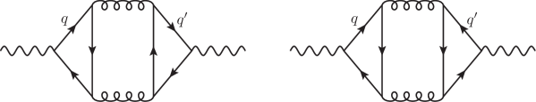
Figure 2.1: Three-loop contribution to the $Z$ boson mass from diagrams involving two triangle quark loops, which give a non-vanishing contribution with a consistent treatment of the axial vector coupling. These contributions are individually divergent for each of $(q,q^{\prime})=(t,t),(t,b),(b,t),(b,b)$, but are finite and gauge invariant after the combination. Contributions involving sums over other $(q,q^{\prime})$ quark doublet combinations vanish in the massless quark limit.

(The vector couplings to the $Z$ boson give vanishing contributions for the sum of these diagrams.) The contributions from $(q,q^{\prime})=(t,t),(t,b),(b,t),(b,b)$ are separately divergent, but their sum is finite and gauge invariant. Therefore, for these diagrams only, one can use the prescription Akyeampong:1973xi ; Larin:1993tq

$$\gamma^{\mu}\gamma_{5}\rightarrow\frac{i}{6}\epsilon^{\mu\nu\rho\sigma}\gamma_{\nu}\gamma_{\rho}\gamma_{\sigma},$$ (2.4)

based on the ’t Hooft-Veltman treatment tHooft:1972fi of $\gamma_{5}$, and then carry out the Lorentz algebra in 4 dimensions before reducing to master integrals in $d$ dimensions. The result is the contribution $\Delta_{Z}^{(3,i)}$ in eq. (2.1). The contributions from diagrams with one or both of $q$ and $q^{\prime}$ summed over the other quark doublets $(u,d)$ and $(c,s)$ vanish, because the axial couplings $a_{q_{L}}-a_{q_{R}}$ for down-type and up-type quarks have the same magnitude and opposite sign, and they are being treated as mass degenerate (specifically, massless). The result for general non-zero $s=Z$ found here reduces to $\Delta_{Z}^{(3,i)}\rightarrow 21\zeta_{3}$ for $s=0$, which agrees with the original calculation in that limit Anselm:1993uq and with the corresponding contribution to the $\rho$ parameter obtained in Avdeev:1994db ; Chetyrkin:1995ix ; Schroder:2005db .

The contributions from the diagrams in which the $Z$ boson couples directly to a single massless (in the present approximation, non-top) quark loop are relatively simple, and can be written as:

$$\Delta_{Z}^{(3,j)} = Z\left(-\frac{44215}{324}+\frac{908}{9}\zeta_{3}+\frac{40}{3}\zeta_{5}+\left[41-\frac{88}{3}\zeta_{3}\right]L_{-Z}-\frac{11}{3}L_{-Z}^{2}\right),$$ (2.5)

$$\Delta_{Z}^{(3,k)} = Z\left(\frac{143}{9}+\frac{148}{3}\zeta_{3}-80\zeta_{5}-L_{-Z}\right),$$ (2.6)

$$\Delta_{Z}^{(3,l)} = \frac{16}{27}Z(7t+3Z)I_{7c}(0,0,0,0,0,t,t)+\frac{16}{243}(128t+43Z)I_{6c}(0,0,0,0,t,t)$$ (2.7)

$$-\frac{8}{27}(18t+7Z)I_{6f}(0,0,0,0,t,t)+\frac{32}{243t}(5Z-17t)I_{5c}(0,0,0,t,t)+\frac{160}{81t}I_{4}(0,0,t,t)$$

$$+\left(\frac{896}{243}\zeta_{3}-\frac{8276}{729}\right)t+\frac{2599}{243}{Z}+\frac{80}{2187}\frac{Z^{2}}{t}+\left(\frac{11144}{243}t-\frac{224}{9}\zeta_{3}t-\frac{3320}{243}Z\right)L_{t}$$

$$-\frac{352}{81}tL_{t}^{2}-\frac{112}{243}tL_{t}^{3}+\frac{4}{243}(884t-217Z)L_{-Z}+\left(\frac{160}{27}Z-\frac{32}{3}t\right)L_{t}L_{-Z}$$

$$+\frac{272}{81}tL_{t}^{2}L_{-Z}+\frac{20}{81}ZL_{-Z}^{2}-\frac{16}{243}(17t+10Z)L_{t}L_{-Z}^{2},$$

$$\Delta_{Z}^{(3,m)} = Z\left(\frac{3701}{81}-\frac{304}{9}\zeta_{3}+\left[\frac{32}{3}\zeta_{3}-\frac{44}{3}\right]L_{-Z}+\frac{4}{3}L_{-Z}^{2}\right).$$ (2.8)

Here, $\Delta_{Z}^{(3,l)}$ contains a top-quark loop that corrects a gluon propagator, rather than connecting to the external $Z$ boson. The remaining contributions in eq. (2.1) are much more complicated, and are given in an ancillary file DeltaZ3 provided with this paper. Each of the contributions has the form of eq. (1.8), with master integrals chosen in ref. Martin:2021pnd :

$${\cal I}^{(1)} = \{\hskip 0.4ptA(t),\>B(0,0),\>B(t,t)\,\},$$ (2.9)

$${\cal I}^{(2)} = \{\hskip 0.4pt\zeta_{3},\,V(t,t,0,t),\,M(t,t,t,t,0),\,M(0,t,0,t,t)\,\},$$ (2.10)

$${\cal I}^{(3)} = \{\hskip 0.4pt\zeta_{5},\,H(0,0,t,0,t,t),\,H(0,t,t,t,0,t),\,I_{4}(t,t,t,t),\,I_{5a}(t,0,t,0,t),\,I_{5b}(0,t,t,t,t),$$ (2.11)

$$I_{5c}(t,t,t,t,t),\,I_{6c}(t,t,t,0,t,t),\,I_{6c2}(t,t,t,0,0,0),\,I_{6d}(0,t,t,t,t,0),\,I_{6d}(t,0,t,0,t,0),$$

$$I_{6d}(t,0,t,t,0,t),\,I_{6e}(0,0,0,0,t,t),\,I_{6e}(0,t,t,t,0,t),\,I_{6e}(t,t,t,0,t,t),\,I_{6f}(0,0,0,0,t,t),\,\phantom{x}$$

$$I_{6f5}(0,0,0,0,t,t),\,I_{7a}(0,0,t,t,t,t,t),\,I_{7a}(t,t,t,t,t,t,0),\,I_{7a3}(t,t,t,t,t,t,0),\,$$

$$I_{7b}(0,t,t,t,t,0,0),\,I_{7b}(t,0,t,t,t,t,0),\,I_{7b4}(t,0,t,t,t,t,0),\,I_{7b4}(t,t,0,t,t,0,t),\,$$

$$I_{7c}(t,t,t,t,0,0,0),\,I_{7d}(t,t,0,t,0,t,0),\,I_{7d}(t,t,0,t,t,0,t),\,I_{7e}(0,0,0,0,0,t,t),\,$$

$$I_{7e}(0,0,t,t,t,0,0),\,I_{8a}(t,0,t,t,t,t,t,0),\,I_{8a}(t,t,t,t,t,0,0,0),\,I_{8b}(t,t,t,t,t,0,0,t),\,$$

$$I_{8c}(t,0,t,t,t,t,t,0),\,I_{8c}^{pk}(t,t,t,t,t,0,0,t)\,\},$$

with $A(t)=t(L_{t}-1)$ and $B(0,0)=2-L_{-Z}$. However, in eq. (2.7) above, I have chosen to write the expression for $\Delta_{Z}^{(3,l)}$ in terms of candidate master integrals that were solved for in ref. Martin:2021pnd , rather than the master integrals listed above (which are a subset of the ones listed in eq. (7.4) in ref. Martin:2021pnd , joined by $B(0,0)$ and $\zeta_{3}$ and $\zeta_{5}$ from the integrals with all propagators massless). This simplifies the expression somewhat, because the integrals used in eq. (2.7) have the same propagator structures as descendants of the underlying Feynman diagrams for the $\Delta_{Z}^{(3,l)}$ contribution.

As a check of eq. (2.1), I have verified that the full expression for the observable $s_{\rm pole}^{Z}$ is renormalization group invariant through 3-loop terms proportional to $g_{3}^{4}$, using the derivatives of the master integrals with respect to $Q$ found in the ancillary file QddQ of ref. Martin:2021pnd .

For practical numerical evaluation, after using the Standard Model group theory values in eq. (1.15), and applying the expansions for the master integrals in the ancillary file Ievenseries of ref. Martin:2021pnd , I find:

$$\Delta_{Z}^{(3),g_{3}^{4}} = g_{3}^{4}t\left\{(g^{2}+g^{\prime 2})(\delta_{1}^{Z}+\delta_{2}^{Z})+a_{u_{L}}a_{u_{R}}\delta_{3}^{Z}+\left[2(a_{u_{L}}^{2}+a_{u_{R}}^{2})+3(a_{d_{L}}^{2}+a_{d_{R}}^{2})\right]\delta_{4}^{Z}\right\},\phantom{xxx}$$ (2.12)

where the series expansions of $\delta_{1}^{Z}$, $\delta_{2}^{Z}$, $\delta_{3}^{Z}$, and $\delta_{4}^{Z}$ are given in the ancillary file DeltaZ3series to order $r_{Z}^{18}$, where

$$r_{Z} \equiv \frac{Z}{4t}\>=\>\frac{g^{2}+g^{\prime 2}}{8y_{t}^{2}}.$$ (2.13)

The contribution $\delta_{1}^{Z}$ isolates the results form the double triangle diagrams in Figure 2.1. The series expansion coefficients are given both numerically, and analytically in terms of $L_{t}$, $L_{-Z}$, and the constants $\zeta_{3}$, $\zeta_{5}$, and

$$c_{H}^{\prime}\>=\>32{\rm Li}_{4}(1/2)-22\zeta_{4}+\frac{4}{3}\ln^{2}(2)[\ln^{2}(2)-\pi^{2})]\>\approx\>-13.2665092775\ldots.$$ (2.14)

The series converge for all $r_{Z}<1$, which is clearly satisfied in actuality. The first few terms in the expansions are

$$\delta_{1}^{Z} = 50.486+r_{Z}\left[79.645+49.333(L_{t}-L_{-Z})+8(L_{t}-L_{-Z})^{2}\right]$$ (2.15)

$$+r_{Z}^{2}\left[-15.758+5.531(L_{t}-L_{-Z})\right]+r_{Z}^{3}\left[-3.066-1.493(L_{t}-L_{-Z})\right]+\ldots$$

$$\delta_{2}^{Z} = 9.978+49.258L_{t}+18L_{t}^{2}-30L_{t}^{3}+r_{Z}\left(-113.200-90.222L_{t}+28L_{t}^{2}\right)$$ (2.16)

$$+r_{Z}^{2}\left(-42.485-63.002L_{t}-4.8L_{t}^{2}\right)$$

$$+r_{Z}^{3}\left(-45.813-74.011L_{t}-32.914L_{t}^{2}\right)+\ldots,$$

$$\delta_{3}^{Z} = r_{Z}\left(-687.728-298.667L_{t}+224L_{t}^{2}\right)+r_{Z}^{2}\left(-733.683-685.827L_{t}-51.200L_{t}^{2}\right)$$ (2.17)

$$+r_{Z}^{3}\left(-707.875-962.072L_{t}-394.971L_{t}^{2}\right)+\ldots,$$

$$\delta_{4}^{Z} = r_{Z}\left(-56.799-14.758L_{t}-10.667L_{t}^{2}+180.381L_{-Z}+21.333L_{t}L_{-Z}-122.667L_{-Z}^{2}\right)$$ (2.18)

$$+r_{Z}^{2}\left[-88.570-33.375(L_{t}-L_{-Z})-3.793(L_{t}-L_{-Z})^{2}\right]$$

$$+r_{Z}^{3}\left[4.074+2.521(L_{t}-L_{-Z})+0.406(L_{t}-L_{-Z})^{2}\right]+\ldots,$$

It is interesting to note that in the expansion in small $r_{Z}$, the sub-leading contribution is numerically comparable to (or even larger than, for smaller $Q$) the leading contribution obtained by $r_{Z}=0$. This is due mostly to the term proportional to $r_{Z}L_{-Z}^{2}$ in the contribution eq. (2.18) from massless quark loops, because of the large magnitude of the coefficient $-122.667$ and because $L_{-Z}^{2}=[-i\pi+\ln(Z/Q^{2})]^{2}$ provides up to an order of magnitude enhancement.

The resulting contribution of eq. (2.12) has now been included in the latest version 1.2 of the code SMDR Martin:2019lqd . Figure 2.2 shows the results for the PDG-convention mass $M_{Z}^{\rm PDG}$ and the width $\Gamma_{Z}$ obtained from the pole mass, for the $\overline{\rm{MS}}$ input parameters given in eq. (1.17).

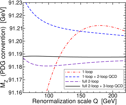
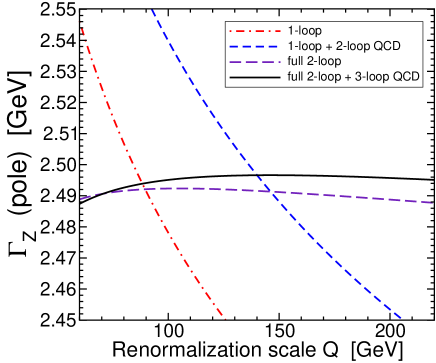
Figure 2.2: The $Z$ boson mass in the PDG convention $M_{Z}^{\rm PDG}$ (left panel) and the width $\Gamma_{Z}$ (right panel), obtained from the calculated complex pole mass $s^{Z}_{\rm pole}$, as a function of the renormalization scale $Q$. The different lines show various approximations as labeled. The $\overline{\rm{MS}}$ input parameters are as given in eq. (1.17), which provide for $M_{Z}^{\rm PDG}=91.1876$ GeV when calculated at the renormalization scale $Q=160$ GeV using the full 2-loop plus 3-loop QCD approximation.

These benchmark parameters were chosen so that the calculated $M_{Z}^{\rm PDG}$, with all known contributions included and using the renormalization scale $Q=160$ GeV, is equal to the experimental central value 91.1876 GeV. To obtain the results in the figure, the $\overline{\rm{MS}}$ input parameters are run to other $\overline{\rm{MS}}$ scales $Q$ using the most complete available renormalization group equations (as listed at the end of the Introduction), and $s_{\rm pole}^{Z}$ is then re-calculated. In the idealized case, the results should not depend on $Q$. I find that with inclusion of the 3-loop QCD corrections, the scale dependence of $M_{Z}$ is remarkably small, less than 0.8 MeV as $Q$ is varied between 50 GeV and 220 GeV. However, given the larger scale dependence found in section IV for the similar case of the $W$ boson mass, I surmise that this very mild scale dependence is partly accidental, and the actual theoretical error due to neglecting higher order contributions is likely to be larger.

The scale dependence of $\Gamma_{Z}$ shown in the right panel of Figure 2.2 is less mild, and not so much improved over the complete 2-loop result, as it varies by a total of about 4 MeV (between minimum and maximum) as $Q$ is varied between 80 GeV and 220 GeV. Note that this determination of $\Gamma_{Z}$ from the complex pole mass (in which the leading contribution arises only as a 1-loop effect) is essentially one loop order less accurate than a direction calculation of the $Z$-boson decay width (in which the leading contribution is a tree-level effect).

III The Higgs boson pole mass

Next, consider the complex pole mass $s^{h}_{\rm pole}$ for the Standard Model Higgs boson, written in the form of eq. (1.1). In this section, I extend the results of ref. Martin:2014cxa to include the momentum-dependent 3-loop self-energy corrections to $\Delta_{h}^{(3)}$ that are proportional to $g_{3}^{4}y_{t}^{2}t$. Also included below are the 3-loop contributions proportional to $g_{3}^{2}y_{t}^{4}t$ and $y_{t}^{6}t$, in an effective potential approximation, which amounts to $g_{3}^{2},y_{t}^{2}\gg\lambda,g^{2},g^{\prime 2}$. For the $y_{t}^{6}t$ part, I provide below an improvement over the result in Martin:2014cxa . Together with the full 2-loop results, these constitute the most complete calculation of the Standard Model Higgs boson mass that is presently available.

The functions $\Delta_{h}^{(1)}$ and the QCD part of $\Delta_{h}^{(2)}$ were given in eqs. (2.46) and (2.47) in ref. Martin:2014cxa , and are evaluated at $s={\rm Re}[s^{h}_{\rm pole}]$, determined by iteration. The remaining, non-QCD part of $\Delta_{h}^{(2)}$ was given in an ancillary file of ref. Martin:2014cxa , where the master integrals were also evaluated at $s={\rm Re}[s^{h}_{\rm pole}]$. However, in the present paper, I adopt a slightly different organization by evaluating the non-QCD part of $\Delta_{h}^{(2)}$ as exactly the same function but evaluated instead at $s=h$, which is consistent up to 3-loop terms of order $y_{t}^{6}t$. This allows an easier extension to 3-loop order, as indicated below.

For the leading QCD part of $\Delta_{h}^{(3)}$ proportional to $g_{3}^{4}y_{t}^{2}t$, the new result can be written in terms of the contributions of four distinct classes of self-energy diagrams characterized by their group theory structures:

$$\Delta_{h}^{(3),g_{3}^{4}y_{t}^{2}t} = g_{3}^{4}y_{t}^{2}N_{c}C_{F}\left(C_{G}\Delta_{h}^{(3,a)}+C_{F}\Delta_{h}^{(3,b)}+T_{F}\Delta_{h}^{(3,c)}+(2n_{g}-1)T_{F}\Delta_{h}^{(3,d)}\right).$$ (3.1)

The results for $\Delta_{h}^{(3,a)}$, $\Delta_{h}^{(3,b)}$, $\Delta_{h}^{(3,c)}$, and $\Delta_{h}^{(3,d)}$ are somewhat lengthy, and so are given in the ancillary file DeltaH3 provided with this paper. They are written in terms of the same list of 3-loop self-energy master integrals as for the $Z$ boson, listed in eqs. (2.9)-(2.11), with the exceptions that $I_{8b}(t,0,t,t,t,t,t,0)$ is also needed in ${\cal I}^{(3)}$, and $\zeta_{5}$, $I_{6e}(0,0,0,0,t,t)$, $I_{6f}(0,0,0,0,t,t)$, $I_{6f5}(0,0,0,0,t,t)$, $I_{7e}(0,0,0,0,0,t,t)$, and $I_{7e}(0,0,t,t,t,0,0)$ are not needed, and of course one should use $s=h$ rather than $s=Z$.

Using the expansions of the master integrals given in ref. Martin:2021pnd , and setting $s=h$ in $\Delta_{h}^{(3),g_{3}^{4}y_{t}^{2}t}$ (which is consistent up to terms of 4-loop order), and plugging in the group theory constants from eq. (1.15), the result becomes a power series in

$$r_{h}\equiv\frac{h}{4t}=\frac{\lambda}{y_{t}^{2}},$$ (3.2)

with coefficients that depend on $L_{t}\equiv\ln(t/Q^{2})$ and $L_{-h}\equiv\ln(h/Q^{2})-i\pi$ and the constants $\zeta_{3}$ and $c_{H}^{\prime}$ from eq. (2.14). The expansion converges for $r_{h}<1$, and does so rapidly for the value realized in the Standard Model. It is given to order $r_{h}^{24}$ in the ancillary file DeltaH3series, both in analytic and numerical forms. The first few terms of the numerical form are:

$$\Delta_{h}^{(3),g_{3}^{4}y_{t}^{2}t} = g_{3}^{4}y_{t}^{2}t\biggl{(}248.122+839.197\,L_{t}+160\,L_{t}^{2}-736\,L_{t}^{3}$$ (3.3)

$$+r_{h}\left[-716.898-1546.064\,L_{t}+336\,L_{t}^{2}+240\,L_{t}^{3}\right]$$

$$+r_{h}^{2}\left[479.663+72.770\,L_{t}+28.444\,L_{-h}\right]$$

$$+r_{h}^{3}\left[-27.675-83.837\,L_{t}-5.486\,L_{t}^{2}+13.274\,L_{-h}\right]+\ldots\biggr{)}.$$

As a non-trivial check, the result obtained with $r_{h}=0$ agrees with that provided in the first line of eq. (3.3) of ref. Martin:2014cxa . The terms with positive powers of $r_{h}$ are new in the present paper.

For the part of $\Delta_{h}^{(3)}$ proportional to $g_{3}^{2}y_{t}^{4}t$, the effective potential approximation gives the second line of eq. (3.3) of ref. Martin:2014cxa , which is not improved on in the present paper, but is reproduced here for reference and comparison:

$$\Delta_{h}^{(3),g_{3}^{2}y_{t}^{4}t} = g_{3}^{2}y_{t}^{4}t\left(2764.365+1283.716\,L_{t}-360\,L_{t}^{2}+240\,L_{t}^{3}\right).$$ (3.4)

It is interesting that $\Delta_{h}^{(3),g_{3}^{4}y_{t}^{2}t}$ is numerically smaller than $\Delta_{h}^{(3),g_{3}^{2}y_{t}^{4}t}$, despite the parametric relative enhancement $N_{c}g_{3}^{2}/y_{t}^{2}$ of the former. In the approximation $r_{h}=0$, this effect was noted in refs. Martin:2014cxa ; Martin:2013gka (see the discussion involving eqs. (6.21)-(6.28) of the former reference) as the result of an unexplained but dramatic near-cancellation, and is found here to be not changed by the inclusion of terms higher order in $r_{h}$.

Finally, for the part of $\Delta_{h}^{(3)}$ proportional to $y_{t}^{6}t$, the effective potential approximation of ref. Martin:2014cxa can be improved on slightly as follows. In the present paper, the non-QCD part of $\Delta_{h}^{(2)}$ is evaluated using master integrals with external momentum invariant $h$ rather than ${\rm Re}[s^{h}_{\rm pole}]$. Then, due to the fortunate circumstance that the leading 1-loop behavior of $s^{h}_{\rm pole}-h$ in the limit $y_{t}^{2}\gg\lambda,g^{2},g^{\prime 2}$ is proportional to $L_{t}$:

$$s^{h}_{\rm pole}-h = \frac{1}{16\pi^{2}}4N_{c}y_{t}^{2}tL_{t},$$ (3.5)

we can fully repair the error in the 3-loop part (caused by using $h$ rather than ${\rm Re}[s^{h}_{\rm pole}]$ in the 2-loop part), simply by requiring renormalization group invariance of the pole mass. This allows inference of the complete dependence proportional to $y_{t}^{6}tL_{t}$, due to the explicit dependence on $Q$. By demanding (and checking) renormalization group invariance of $s_{\rm pole}^{h}$ through terms of 3-loop order in the approximation $g_{3}^{2},y_{t}^{2}\gg\lambda,g^{2},g^{\prime 2}$, I find that the end result for the leading non-QCD 3-loop contribution is that eq. (3.4) of ref. Martin:2014cxa should be replaced by:

$$\Delta_{M_{h}^{2}}^{(3),y_{t}^{6}t} = y_{t}^{6}t\Bigl{[}-3433.724-2426.808L_{t}-101.016L_{t}^{2}-360L_{t}^{3}+L_{h}\left(36+648L_{t}+324L_{t}^{2}\right)\Bigr{]},\phantom{xxx}$$ (3.6)

where the analytic forms of the decimal coefficients are

$$-3433.724 \approx -673-\frac{17\pi^{2}}{2}-1962\zeta_{3}+24c_{H}^{\prime},\phantom{xxxx}$$ (3.7)

$$-2426.808 \approx -\frac{10491}{4}+144\sqrt{3}\pi-42\pi^{2}-144\zeta_{3},$$ (3.8)

$$-101.016 \approx -\frac{855}{2}+60\sqrt{3}\pi.$$ (3.9)

This result differs from eq. (3.4) of ref. Martin:2014cxa by terms that vanish when $L_{t}=0$, consistent with the approximation made in that reference.

To recapitulate: in order to consistently include the 3-loop results given above, the non-QCD part of $\Delta_{h}^{(2)}$ found in the ancillary file of ref. Martin:2014cxa should use $s=h$ in the evaluation of the integrals, while $\Delta_{h}^{(1)}$ and the QCD part of $\Delta_{h}^{(2)}$ provided in that reference should use $s={\rm Re}[s^{h}_{\rm pole}]$ determined by iteration. All of these results for the Higgs boson pole mass have now been implemented in version 1.2 of the computer code SMDR Martin:2019lqd . Figure 3.1 shows the results for $M_{h}$, for the benchmark $\overline{\rm{MS}}$ input parameters given in eq. (1.17).

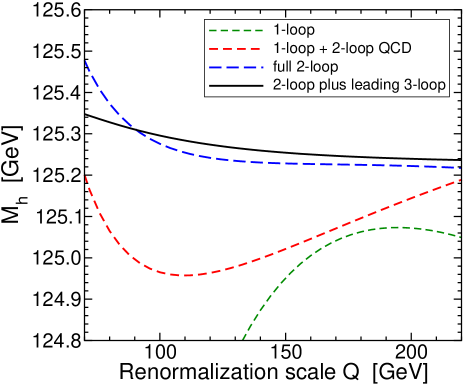
Figure 3.1: The real part of the calculated Higgs boson pole mass, as a function of the renormalization scale $Q$. The different lines show various approximations as labeled. The $\overline{\rm{MS}}$ input parameters are as given in eq. (1.17), which provide for $M_{h}=125.25$ GeV when calculated at the renormalization scale $Q=160$ GeV with the best available approximation as described in the text.

Recall that these parameters were chosen so as to give the present experimental central value from the RPP, $M_{h}=125.25$ GeV, as the result of the calculation at renormalization scale $Q=160$ GeV. The other results in the figure were obtained by running the $\overline{\rm{MS}}$ parameters in eq. (1.17) from the input scale $Q_{0}=172.5$ GeV to each scale $Q$ and re-doing the calculation. The new contributions found in this paper give the best approximation available at this writing, but still imply a scale dependence of several tens of MeV. For example, the calculated $M_{h}$ decreases by about 56 MeV when $Q$ is varied from 100 GeV to 200 GeV, for fixed values of the $\overline{\rm{MS}}$ input parameters. This provides a lower bound on the theoretical error, and suggests that a still more refined calculation of the Higgs pole mass, to include 3-loop electroweak parts and even leading 4-loop contributions, would be worthwhile, since the experimental uncertainty on $M_{h}$ from future collider experiments may well be smaller deBlas:2019rxi . It is also possible R:2021bml to refine further the gaugeless limit by including momentum-dependent parts of the Higgs boson self-energy function.

A famous feature of the observed Higgs boson mass is that the Standard Model with no extensions can then have the Higgs self-coupling $\lambda$ run negative at a scale that is far above the electroweak scale but below the Planck scale, implying a possibly metastable electroweak vacuum. This is illustrated in Figure 3.2, using the latest experimental values and the results of this paper to relate $M_{h}$ to $\lambda$ in the most accurate available way.

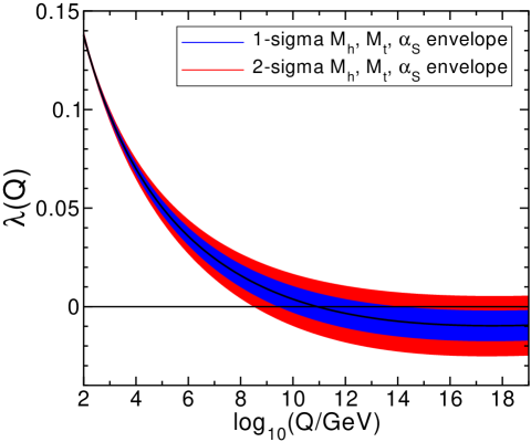
Figure 3.2: The running Higgs self-coupling parameter $\lambda$ as a function of the $\overline{\rm{MS}}$ renormalization scale $Q$, using the results of this paper to relate it to $M_{h}$ in the most accurate available way. The central value obtained from the present experimental data as in eqs. (1.16) and (1.17) is the black line. The shaded envelopes are the envelopes obtained by varying $M_{h}=125.25\pm 0.17$ GeV, $M_{t}=172.5\pm 0.7$ GeV, and $\alpha_{S}^{(5)}(M_{Z})=0.1179\pm 0.0010$ in their 1-sigma and 2-sigma ranges.

As is well-known (see for example refs. EliasMiro:2011aa and Bezrukov:2012sa ; Degrassi:2012ry ; Buttazzo:2013uya ), the scale of possible instability is lowered if the top-quark mass is higher, or the QCD coupling is lower, or the Higgs mass is lower, than their benchmark values, while it is possible for the instability to be avoided up to the Planck scale if the deviations are in the opposite directions. While improved formulas and experimental values for $M_{h}$ are welcome, the dominant uncertainty in these instability discussions comes from $M_{t}$ (or $y_{t}$), and the second most important uncertainty is that of $\alpha_{S}^{(5)}(M_{Z})$, through their renormalization group running influence on $\lambda$.

IV The $W$ boson pole mass

Consider the $W$-boson complex pole squared mass $s^{W}_{\rm pole}$ as in eq. (1.1). The complete 1-loop and 2-loop parts $\Delta_{W}^{(1)}$ and $\Delta_{W}^{(2)}$ were given in ref. Martin:2015lxa . The 3-loop QCD part splits into 8 distinct contributions with different group theory structures:

$$\Delta_{W}^{(3),g_{3}^{4}} = g_{3}^{4}g^{2}N_{c}C_{F}\biggl{(}C_{G}\left[\Delta_{W}^{(3,a)}+(n_{g}-1)\Delta_{W}^{(3,b)}\right]+C_{F}\left[\Delta_{W}^{(3,c)}+(n_{g}-1)\Delta_{W}^{(3,d)}\right]$$ (4.1)

$$+T_{F}\left[\Delta_{W}^{(3,e)}+(n_{g}-1)\Delta_{W}^{(3,f)}+(2n_{g}-1)\Delta_{W}^{(3,g)}+(2n_{g}-1)(n_{g}-1)\Delta_{W}^{(3,h)}\right]\biggr{)}.\phantom{xxx}$$

The four contributions from diagrams in which the $W$ boson couples directly to massless quarks are relatively simple:

$$\Delta_{W}^{(3,b)} = W\left(-\frac{44215}{648}+\frac{454}{9}\zeta_{3}+\frac{20}{3}\zeta_{5}+\left[\frac{41}{2}-\frac{44}{3}\zeta_{3}\right]L_{-W}-\frac{11}{6}L_{-W}^{2}\right),$$ (4.2)

$$\Delta_{W}^{(3,d)} = W\left(\frac{143}{18}+\frac{74}{3}\zeta_{3}-40\zeta_{5}-\frac{1}{2}L_{-W}\right),$$ (4.3)

$$\Delta_{W}^{(3,f)} = \frac{8}{27}W(7t+3W)I_{7c}(0,0,0,0,0,t,t)+\frac{8}{243}(128t+43W)I_{6c}(0,0,0,0,t,t)$$ (4.4)

$$-\frac{4}{27}(18t+7W)I_{6f}(0,0,0,0,t,t)+\frac{16}{243t}(5W-17t)I_{5c}(0,0,0,t,t)+\frac{80}{81t}I_{4}(0,0,t,t)$$

$$+\left(\frac{448}{243}\zeta_{3}-\frac{4138}{729}\right)t+\frac{2599}{486}{W}+\frac{40}{2187}\frac{W^{2}}{t}+\left(\frac{5572}{243}t-\frac{112}{9}\zeta_{3}t-\frac{1660}{243}W\right)L_{t}$$

$$-\frac{176}{81}tL_{t}^{2}-\frac{56}{243}tL_{t}^{3}+\frac{2}{243}(884t-217W)L_{-W}+\left(\frac{80}{27}W-\frac{16}{3}t\right)L_{t}L_{-W}$$

$$+\frac{136}{81}tL_{t}^{2}L_{-W}+\frac{10}{81}WL_{-W}^{2}-\frac{8}{243}(17t+10W)L_{t}L_{-W}^{2},$$

$$\Delta_{W}^{(3,h)} = W\left(\frac{3701}{162}-\frac{152}{9}\zeta_{3}+\left[\frac{16}{3}\zeta_{3}-\frac{22}{3}\right]L_{-W}+\frac{2}{3}L_{-W}^{2}\right).$$ (4.5)

In fact, $\Delta_{W}^{(3,b)}$, $\Delta_{W}^{(3,d)}$, $\Delta_{W}^{(3,f)}$, and $\Delta_{W}^{(3,h)}$ can be obtained from, respectively, $\Delta_{Z}^{(3,j)}$, $\Delta_{Z}^{(3,k)}$, $\Delta_{Z}^{(3,l)}$, and $\Delta_{Z}^{(3,m)}$ in eqs. (2.5)-(2.8) by replacing $Z\rightarrow W$ and dividing by 2. The reason for this is that they come from exactly the same Feynman diagram topologies.

The remaining four contributions $\Delta_{W}^{(3,a)}$, $\Delta_{W}^{(3,c)}$, $\Delta_{W}^{(3,e)}$, and $\Delta_{W}^{(3,g)}$ in eq. (4.1) are more complicated, and are relegated to an ancillary file DeltaW3. They each have the form of eq. (1.8), with renormalized $\epsilon$-finite master integrals that are a subset of eqs. (6.2)-(6.4) of ref. Martin:2021pnd :

$${\cal I}^{(1)} = \{\hskip 0.4ptA(t),\>B(0,t)\hskip 0.4pt\},$$ (4.6)

$${\cal I}^{(2)} = \{\hskip 0.4ptS(0,0,t),\,S(t,t,t),\,U(t,0,t,t),\,M(0,0,t,t,0)\hskip 0.4pt\},$$ (4.7)

$${\cal I}^{(3)} = \{\hskip 0.4ptH(0,t,t,t,0,t),\,I_{4}(0,t,t,t),\,I_{6d}(0,0,t,0,t,0),\,I_{6d}(0,0,t,t,0,t),\,I_{6d}(t,0,0,0,0,0),$$ (4.8)

$$I_{6e}(0,t,0,0,0,t),\,I_{6e}(t,0,t,0,0,t),\,I_{6f}(0,t,t,0,0,t),\,I_{6f1}(t,0,0,t,0,t),$$

$$I_{7a}(0,0,0,0,t,t,t),\,I_{7a}(0,0,t,t,0,0,0),\,I_{7a}(0,t,t,0,0,t,0),\,I_{7a}(t,t,0,0,t,t,0),$$

$$I_{7a5}(t,t,0,0,t,t,0),\,I_{7b}(0,0,t,0,t,0,0),\,I_{7c}(0,0,t,t,0,0,0),\,I_{7d}(0,t,0,t,t,0,t),$$

$$I_{7e}(0,t,t,0,0,0,0),\,I_{8b}(0,0,0,t,t,0,0,t),\,I_{8c}(0,0,0,t,t,0,0,t),\,I_{8c}^{pk}(t,t,t,0,0,0,0,0)\hskip 0.4pt\}.\phantom{xxxx}$$

I have checked that eq. (4.1) gives a pole mass $s^{W}_{\rm pole}$ that is renormalization group invariant through 3-loop terms of order $g_{3}^{4}$, using the derivatives of the master integrals with respect to $Q$ found in the ancillary file QddQ of ref. Martin:2021pnd .

For practical numerical evaluation, after plugging in the Standard Model group theory values in eq. (1.15), and applying the expansions for the master integrals in the ref. Martin:2021pnd ancillary files Ioddseries and Ievenseries (the latter being needed only for the contribution $\Delta_{W}^{(3,f)}$ in which the $W$ boson couplings are to a massless quark loop, with a top-quark loop correcting a gluon propagator), I obtain a series expansion:

$$\Delta_{W}^{(3),g_{3}^{4}} = g_{3}^{4}\,g^{2}t\left(\delta_{1}^{W}+\delta_{2}^{W}\right),$$ (4.9)

where $\delta_{1}^{W}$ comes from $\Delta_{W}^{(3,a)}$, $\Delta_{W}^{(3,c)}$, $\Delta_{W}^{(3,e)}$, and $\Delta_{W}^{(3,g)}$, which follow from diagrams where the $W$ boson couples directly to a top-bottom pair, and $\delta_{2}^{W}$ comes from $\Delta_{W}^{(3,b)}$, $\Delta_{W}^{(3,d)}$, $\Delta_{W}^{(3,f)}$, and $\Delta_{W}^{(3,h)}$ from diagrams in which the $W$ boson couples directly to light-quark pairs. An ancillary file DeltaW3series provided with this paper gives the results, both analytically and numerically, to orders $\rho_{W}^{30}$ and $r_{W}^{16}$, where

$$\rho_{W} \equiv \frac{W}{t}\,=\,\frac{g^{2}}{2y_{t}^{2}}\qquad\mbox{and}\qquad r_{W}=\frac{\rho_{W}}{4},$$ (4.10)

and the coefficients involve $L_{t}=\ln(t/Q^{2})$ and $L_{-W}=\ln(W/Q^{2})-i\pi=2-B(0,0)\bigl{|}_{s=W+i\epsilon}$, as well as $\zeta_{2}$, $\zeta_{3}$, $\zeta_{4}$, $\zeta_{5}$, $c_{H}^{\prime}$ from eq. (2.14), and

$$c_{I} = \sqrt{3}\,{\rm Im}\left[{\rm Li}_{2}(e^{2\pi i/3})\right]\>\approx\>1.1719536193\ldots.$$ (4.11)

Note that $\delta_{2}^{W}$ is the same as $\delta_{4}^{Z}$ appearing in eqs. (2.12) (2.18) with the replacement $r_{Z}\rightarrow r_{W}$. The series for $\delta_{1}^{W}$ and $\delta_{2}^{W}$ converge for $\rho_{W}<1$ and $r_{W}<1$, respectively, which is clearly satisfied by the relevant value of $W/t$ in the Standard Model.

The numerical form of the first few terms in the series are

$$\delta_{1}^{W} = 12.8299+24.9541L_{t}+63L_{t}^{2}-30L_{t}^{3}\,+\,\rho_{W}(-23.800-54.693L_{t}+14L_{t}^{2})$$ (4.12)

$$+\rho_{W}^{2}(-2.327-17.873L_{t}-1.5L_{t}^{2})\,+\,\rho_{W}^{3}(-0.700-7.496L_{t}-7.2L_{t}^{2})+\ldots,\phantom{xxx}$$

$$\delta_{2}^{W} = r_{W}\left(-56.799-14.758L_{t}-10.667L_{t}^{2}+180.381L_{-W}+21.333L_{t}L_{-W}-122.667L_{-W}^{2}\right)$$ (4.13)

$$+r_{W}^{2}\left[-88.570-33.375(L_{t}-L_{-W})-3.793(L_{t}-L_{-W})^{2}\right]$$

$$+r_{W}^{3}\left[4.074+2.521(L_{t}-L_{-W})+0.406(L_{t}-L_{-W})^{2}\right]+\ldots.$$

As in the case of the $Z$ boson, it is interesting to note that in this expansion in small $W/t$, the sub-leading contribution is numerically comparable to or larger than the leading contribution (obtained by $\rho_{W}=r_{W}=0$), depending on the choice of $Q$. This is due mostly to the term proportional to $r_{W}L_{-W}^{2}$ in the contribution from massless quark loops, because of the large magnitude of the coefficient $-122.667$ and because $L_{-W}^{2}=[-i\pi+\ln(W/Q^{2})]^{2}$ provides up to an order of magnitude enhancement.

The contribution $\Delta_{W}^{(3),g_{3}^{4}}$ is now implemented in the new version 1.2 of the computer code SMDR Martin:2019lqd . Figure 4.1 shows the results for $M_{W}^{\rm PDG}$ and for $\Gamma_{W}$ obtained from the complex pole squared mass $s_{\rm pole}^{W}$, for the $\overline{\rm{MS}}$ input parameters in eq. (1.17) at the reference scale $Q_{0}=172.5$ GeV.

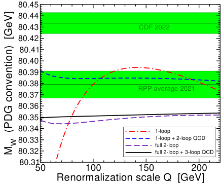
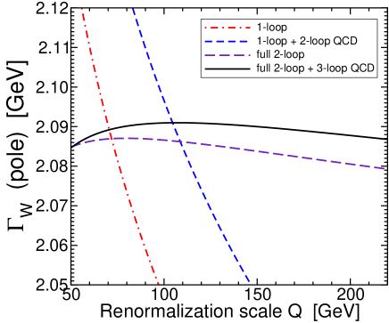
Figure 4.1: The PDG convention $W$ boson mass, and the width $\Gamma_{W}$, obtained from the calculated complex pole mass $s^{W}_{\rm pole}$, as a function of the renormalization scale $Q$. The different lines show various approximations as labeled. The $\overline{\rm{MS}}$ input parameters are as given in eq. (1.17). Also shown are the experimental central values and $1\sigma$ ranges for $M_{W}^{\rm PDF}$ as given by the 2021 update to the 2020 RPP, and from the 2022 result from CDF CDF:2022hxs with statistical and systematic errors combined in quadrature.

The default scale used by SMDR v1.2 for the $W$ mass calculation is $Q=160$ GeV, which gives $M_{W}^{\rm PDG}=80.3525$ GeV and $\Gamma_{W}=2.0896$ GeV. The results for other renormalization scales $Q$ are obtained by first running the $\overline{\rm{MS}}$ parameters to $Q$ and then re-calculating $s_{\rm pole}^{W}$. The three-loop QCD contribution to $M_{W}^{\rm PDG}$ is seen to be as large as about 6 MeV. In the idealized case, the total $s_{\rm pole}^{W}$ would not depend on $Q$. The computed value of $M_{W}^{\rm PDG}$ varies by less than 2.4 MeV as $Q$ is varied from 80 GeV to 180 GeV. This is significantly larger than the scale dependence of the computed $M_{Z}^{\rm PDG}$ as found in Figure 2.2, but compares quite favorably to the present experimental uncertainty of 12 MeV. The range for $M_{W}^{\rm PDG}$ from the average of experimental data released through 2021 is $80.379\pm 0.012$ GeV. The CDF collaboration has recently produced a result that is substantially higher, $80.4335\pm 0.0064_{\rm stat}\pm 0.0069_{\rm syst}$ GeV, which is in stark disagreement with the Standard Model prediction. These results are also shown in Figure 4.1. As seen in the right panel of Figure 4.1, the total variation in $\Gamma_{W}$ as $Q$ varies from 60 GeV to 220 GeV is about 3.5 MeV, but the spread is only about 2.3 MeV as $Q$ varies from 80 GeV to 180 GeV. These scale variations are improved over the full 2-loop order calculation found in ref. Martin:2015lxa . For comparison, the largest parametric uncertainty contributing to the $M_{W}$ prediction is that of the top-quark pole mass $M_{t}$. If one fixes eqs. (1.16) and (1.17) as a reference model, and then adjusts the Standard Model inputs to fit varying $M_{t},M_{Z},\Delta\alpha_{\rm had}^{(5)}$, and $\alpha_{S}^{(5)}(M_{Z})$, then one finds approximately

$$M_{W}^{\rm PDG} = M_{W}^{\rm PDG,ref}+\mbox{6.1 MeV}\left(\frac{M_{t}-M_{t}^{\rm ref}}{\rm GeV}\right)+\mbox{1.3 MeV}\left(\frac{M_{Z}^{\rm PDG}-M_{Z}^{\rm PDG,ref}}{\rm MeV}\right)$$ (4.14)

$$-\mbox{1.8 MeV}\left(\frac{\Delta\alpha^{(5)}_{\rm had}-\Delta\alpha_{\rm had}^{(5),{\rm ref}}}{0.0001}\right)-\mbox{0.7 MeV}\left(\frac{\alpha_{S}^{(5)}(M_{Z})-\alpha_{S}^{(5)}(M_{Z})^{\rm ref}}{0.001}\right)$$

as the prediction for the $W$ boson mass in the PDG convention, with $M_{W}^{\rm PDG,ref}=80.3525$ GeV.

In Figure 4.2, I compare the prediction for $M_{W}^{\rm PDF}$ from SMDR v1.2 (incorporating the results of this paper) in the pure $\overline{\rm{MS}}$ scheme to the corresponding results in the on-shell scheme using the interpolation formula in ref. Awramik:2003rn , and to those in the hybrid $\overline{{\rm MS}}$-on-shell scheme of ref. Degrassi:2014sxa , as a function of the top-quark pole mass. The other on-shell parameters $M_{Z}^{\rm PDG}$, $G_{\mu}$, $\alpha^{(5)}_{S}(M_{Z})$, $\Delta\alpha_{\rm had}^{(5)}$, and $M_{h}$ are chosen to be the same, and equal to the data given in from eq. (1.16) from the 2021 update to the 2020 RPP, so that the results are directly comparable. (In the $\overline{\rm{MS}}$ scheme, this entails doing a fit to determine the Lagrangian parameters, which is readily accomplished using the C function SMDR_Fit_Inputs or the interactive command-line tool calc_fit -int.) The pure $\overline{\rm{MS}}$ scheme gives results between those of the on-shell and hybrid schemes, with a total spread between the three schemes of about 4.5 MeV.

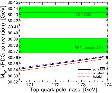
Figure 4.2: Comparison of Standard Model predictions for the $W$ boson mass in the PDG convention, as a function of the top-quark pole mass $M_{t}$, using data for $M_{Z}^{\rm PDG}$, $G_{\mu}$, $\alpha^{(5)}_{S}(M_{Z})$, $\Delta\alpha_{\rm had}^{(5)}$, and $M_{h}$ from eq. (1.16). The solid black line is the pure $\overline{\rm{MS}}$ scheme result, obtained using SMDR v1.2 incorporating the results of this paper. The short dashed (blue) line is the on-shell scheme result, obtained from the interpolating formula in ref. Awramik:2003rn . The long dashed (red) line is the result from the hybrid $\overline{\rm MS}$-on-shell scheme of ref. Degrassi:2014sxa . Also shown are the experimental central values and $1\sigma$ ranges for $M_{W}^{\rm PDF}$ as given by the 2021 update to the 2020 RPP, and from the 2022 result from CDF CDF:2022hxs .

V Outlook

In this paper, I have reported the 3-loop QCD contributions to the $W$, $Z$, and Higgs boson physical masses in the Standard Model, in the pure $\overline{\rm{MS}}$ renormalization scheme with a tadpole-free treatment of the Higgs VEV. The results show improved renormalization group scale independence, especially for the $W$ and $Z$ boson cases, and in all three cases the scale variation is less than the present experimental uncertainty. Alternative methods based on on-shell type schemes have already included 4-loop QCD contributions through the rho parameter, but it is not clear that these should be numerically more important than 3-loop mixed and pure electroweak contributions. The results of this paper have all been incorporated in the latest version 1.2 of the code SMDR Martin:2019lqd . Further improvements in the approach of the present paper could come from computing all of the remaining 3-loop self-energy contributions to the pole masses, which in the case of the most general diagrams will be a challenging but perhaps not insurmountable goal.

Acknowledgments: I thank Scott Willenbrock for useful conversations regarding the parameterization of complex pole masses. This work was supported in part by the National Science Foundation grant number 2013340.

References

- (1) W. A. Bardeen, A. J. Buras, D. W. Duke and T. Muta, “Deep Inelastic Scattering Beyond the Leading Order in Asymptotically Free Gauge Theories,” Phys. Rev. D 18, 3998 (1978).
- (2) E. Braaten and J. P. Leveille, “Minimal Subtraction and Momentum Subtraction in QCD at Two Loop Order,” Phys. Rev. D 24, 1369 (1981).
- (3) C. G. Bollini and J. J. Giambiagi, “Dimensional Renormalization: The Number of Dimensions as a Regularizing Parameter,” Nuovo Cim. B 12, 20 (1972). C. G. Bollini and J. J. Giambiagi, “Lowest order divergent graphs in nu-dimensional space,” Phys. Lett. B 40, 566 (1972).
- (4) J. F. Ashmore, “A Method of Gauge Invariant Regularization,” Lett. Nuovo Cim. 4, 289 (1972).
- (5) G. M. Cicuta and E. Montaldi, “Analytic renormalization via continuous space dimension,” Lett. Nuovo Cim. 4, 329 (1972).
- (6) G. ’t Hooft and M. J. G. Veltman, “Regularization and Renormalization of Gauge Fields,” Nucl. Phys. B 44, 189 (1972).
- (7) G. ’t Hooft, “Dimensional regularization and the renormalization group,” Nucl. Phys. B 61, 455 (1973).
- (8) C. Ford, I. Jack and D. R. T. Jones, Nucl. Phys. B 387, 373-390 (1992) [erratum: Nucl. Phys. B 504, 551-552 (1997)] [arXiv:hep-ph/0111190 [hep-ph]].
- (9) S. P. Martin, “Two Loop Effective Potential for a General Renormalizable Theory and Softly Broken Supersymmetry,” Phys. Rev. D 65, 116003 (2002) [arXiv:hep-ph/0111209 [hep-ph]].
- (10) S. P. Martin, “Three-Loop Standard Model Effective Potential at Leading Order in Strong and Top Yukawa Couplings,” Phys. Rev. D 89, no.1, 013003 (2014) [arXiv:1310.7553 [hep-ph]].
- (11) S. P. Martin, “Effective potential at three loops,” Phys. Rev. D 96, no. 9, 096005 (2017) [arXiv:1709.02397 [hep-ph]].
- (12) S. P. Martin, “Four-loop Standard Model effective potential at leading order in QCD,” Phys. Rev. D 92, no. 5, 054029 (2015) [arXiv:1508.00912 [hep-ph]].
- (13) S. P. Martin, “Taming the Goldstone contributions to the effective potential,” Phys. Rev. D 90, no.1, 016013 (2014) [arXiv:1406.2355 [hep-ph]].
- (14) J. Elias-Miro, J. R. Espinosa and T. Konstandin, “Taming Infrared Divergences in the Effective Potential,” JHEP 08, 034 (2014) [arXiv:1406.2652 [hep-ph]].
- (15) F. Jegerlehner, M. Y. Kalmykov and O. Veretin, “MS versus pole masses of gauge bosons: Electroweak bosonic two loop corrections,” Nucl. Phys. B 641, 285 (2002) [hep-ph/0105304].
- (16) F. Jegerlehner, M. Y. Kalmykov and O. Veretin, “MS-bar versus pole masses of gauge bosons. 2. Two loop electroweak fermion corrections,” Nucl. Phys. B 658, 49 (2003) [hep-ph/0212319].
- (17) G. Degrassi, P. Gambino and P. P. Giardino, “The interdependence in the Standard Model: a new scrutiny,” JHEP 1505, 154 (2015) [arXiv:1411.7040 [hep-ph]].
- (18) B. A. Kniehl, A. F. Pikelner and O. L. Veretin, “Two-loop electroweak threshold corrections in the Standard Model,” Nucl. Phys. B 896, 19 (2015) [arXiv:1503.02138 [hep-ph]].
- (19) J. J. van der Bij and F. Hoogeveen, “Two Loop Correction to Weak Interaction Parameters Due to a Heavy Fermion Doublet,” Nucl. Phys. B 283, 477 (1987). doi:10.1016/0550-3213(87)90284-7
- (20) A. Djouadi and C. Verzegnassi, “Virtual Very Heavy Top Effects in LEP / SLC Precision Measurements,” Phys. Lett. B 195, 265 (1987). doi:10.1016/0370-2693(87)91206-8
- (21) A. Djouadi, “O(alpha alpha-s) Vacuum Polarization Functions of the Standard Model Gauge Bosons,” Nuovo Cim. A 100, 357 (1988). doi:10.1007/BF02812964
- (22) B. A. Kniehl, “Two Loop Corrections to the Vacuum Polarizations in Perturbative QCD,” Nucl. Phys. B 347, 86 (1990). doi:10.1016/0550-3213(90)90552-O
- (23) F. Halzen and B. A. Kniehl, “ r beyond one loop,” Nucl. Phys. B 353, 567 (1991). doi:10.1016/0550-3213(91)90319-S
- (24) R. Barbieri, M. Beccaria, P. Ciafaloni, G. Curci and A. Vicere, “Radiative correction effects of a very heavy top,” Phys. Lett. B 288, 95 (1992) Erratum: [Phys. Lett. B 312, 511 (1993)] [hep-ph/9205238].
- (25) A. Djouadi and P. Gambino, “Electroweak gauge bosons selfenergies: Complete QCD corrections,” Phys. Rev. D 49, 3499 (1994) Erratum: [Phys. Rev. D 53, 4111 (1996)] [hep-ph/9309298].
- (26) J. Fleischer, O. V. Tarasov and F. Jegerlehner, “Two loop heavy top corrections to the rho parameter: A Simple formula valid for arbitrary Higgs mass,” Phys. Lett. B 319, 249 (1993). doi:10.1016/0370-2693(93)90810-5
- (27) L. Avdeev, J. Fleischer, S. Mikhailov and O. Tarasov, “ correction to the electroweak rho parameter,” Phys. Lett. B 336, 560 (1994) [Phys. Lett. B 349, 597 (1995)] [hep-ph/9406363].
- (28) K. G. Chetyrkin, J. H. Kühn and M. Steinhauser, “Corrections of order to the parameter,” Phys. Lett. B 351, 331 (1995) [hep-ph/9502291].
- (29) K. G. Chetyrkin, J. H. Kühn and M. Steinhauser, “QCD corrections from top quark to relations between electroweak parameters to order alpha-s**2,” Phys. Rev. Lett. 75, 3394 (1995) [hep-ph/9504413].
- (30) G. Degrassi, P. Gambino and A. Vicini, “Two loop heavy top effects on the m(Z) - m(W) interdependence,” Phys. Lett. B 383, 219 (1996) [hep-ph/9603374].
- (31) A. Freitas, W. Hollik, W. Walter and G. Weiglein, “Complete fermionic two loop results for the M(W) - M(Z) interdependence,” Phys. Lett. B 495, 338 (2000) Erratum: [Phys. Lett. B 570, no. 3-4, 265 (2003)] [hep-ph/0007091].
- (32) J. J. van der Bij, K. G. Chetyrkin, M. Faisst, G. Jikia and T. Seidensticker, “Three loop leading top mass contributions to the rho parameter,” Phys. Lett. B 498, 156 (2001) [hep-ph/0011373].
- (33) A. Freitas, W. Hollik, W. Walter and G. Weiglein, “Electroweak two loop corrections to the mass correlation in the standard model,” Nucl. Phys. B 632, 189 (2002) Erratum: [Nucl. Phys. B 666, 305 (2003)] [hep-ph/0202131].
- (34) M. Awramik and M. Czakon, “Complete two loop bosonic contributions to the muon lifetime in the standard model,” Phys. Rev. Lett. 89, 241801 (2002) [hep-ph/0208113].
- (35) A. Onishchenko and O. Veretin, “Two loop bosonic electroweak corrections to the muon lifetime and M(Z) - M(W) interdependence,” Phys. Lett. B 551, 111 (2003) [hep-ph/0209010].
- (36) M. Faisst, J. H. Kühn, T. Seidensticker and O. Veretin, “Three loop top quark contributions to the rho parameter,” Nucl. Phys. B 665, 649 (2003) [hep-ph/0302275].
- (37) M. Awramik and M. Czakon, “Complete two loop electroweak contributions to the muon lifetime in the standard model,” Phys. Lett. B 568, 48 (2003) [hep-ph/0305248].
- (38) M. Awramik, M. Czakon, A. Freitas and G. Weiglein, “Precise prediction for the W boson mass in the standard model,” Phys. Rev. D 69, 053006 (2004) [hep-ph/0311148].
- (39) Y. Schroder and M. Steinhauser, “Four-loop singlet contribution to the rho parameter,” Phys. Lett. B 622, 124 (2005) [hep-ph/0504055].
- (40) K. G. Chetyrkin, M. Faisst, J. H. Kuhn, P. Maierhofer and C. Sturm, “Four-Loop QCD Corrections to the Rho Parameter,” Phys. Rev. Lett. 97, 102003 (2006) [hep-ph/0605201].
- (41) R. Boughezal and M. Czakon, “Single scale tadpoles and O(G(F m(t)**2 alpha(s)**3)) corrections to the rho parameter,” Nucl. Phys. B 755, 221 (2006) [hep-ph/0606232].
- (42) S. P. Martin, “Pole Mass of the W Boson at Two-Loop Order in the Pure Scheme,” Phys. Rev. D 91, no. 11, 114003 (2015) [arXiv:1503.03782 [hep-ph]].
- (43) S. P. Martin, “-Boson Pole Mass at Two-Loop Order in the Pure Scheme,” Phys. Rev. D 92, no.1, 014026 (2015) [arXiv:1505.04833 [hep-ph]].
- (44) F. Bezrukov, M. Y. Kalmykov, B. A. Kniehl and M. Shaposhnikov, “Higgs Boson Mass and New Physics,” JHEP 1210, 140 (2012) [arXiv:1205.2893 [hep-ph]].
- (45) G. Degrassi, S. Di Vita, J. Elias-Miro, J. R. Espinosa, G. F. Giudice, G. Isidori and A. Strumia, “Higgs mass and vacuum stability in the Standard Model at NNLO,” JHEP 1208, 098 (2012) [arXiv:1205.6497 [hep-ph]].
- (46) D. Buttazzo, G. Degrassi, P. P. Giardino, G. F. Giudice, F. Sala, A. Salvio and A. Strumia, “Investigating the near-criticality of the Higgs boson,” JHEP 1312, 089 (2013) [arXiv:1307.3536 [hep-ph]].
- (47) S. P. Martin and D. G. Robertson, “Higgs boson mass in the Standard Model at two-loop order and beyond,” Phys. Rev. D 90, no. 7, 073010 (2014) [arXiv:1407.4336 [hep-ph]].
- (48) S. P. Martin, “Evaluation of two loop selfenergy basis integrals using differential equations,” Phys. Rev. D 68, 075002 (2003) [arXiv:hep-ph/0307101 [hep-ph]].
- (49) S. P. Martin and D. G. Robertson, “TSIL: A Program for the calculation of two-loop self-energy integrals,” Comput. Phys. Commun. 174, 133-151 (2006) [arXiv:hep-ph/0501132 [hep-ph]].
- (50) S. P. Martin and D. G. Robertson, “Standard model parameters in the tadpole-free pure scheme,” Phys. Rev. D 100, no.7, 073004 (2019) [arXiv:1907.02500 [hep-ph]]. The latest version of the SMDR code can be downloaded from: http://www.niu.edu/spmartin/SMDR/
- (51) B. A. Kniehl, A. F. Pikelner and O. L. Veretin, “mr: a C++ library for the matching and running of the Standard Model parameters,” Comput. Phys. Commun. 206, 84 (2016) [arXiv:1601.08143 [hep-ph]].
- (52) P.A. Zyla et al. [Particle Data Group], “Review of Particle Physics,” PTEP 2020, no.8, 083C01 (2020) with 2021 updates at https://pdg.lbl.gov/
- (53) S. Willenbrock, “Mass and width of an unstable particle,” [arXiv:2203.11056 [hep-ph]].
- (54) T. Aaltonen et al. [CDF], “High-precision measurement of the W boson mass with the CDF II detector,” Science 376, no.6589, 170-176 (2022) doi:10.1126/science.abk1781
- (55) S. P. Martin, “Renormalized -finite master integrals and their virtues: the three-loop self energy case,” [arXiv:2112.07694 [hep-ph]].
- (56) M. E. Machacek and M. T. Vaughn, “Two Loop Renormalization Group Equations in a General Quantum Field Theory. 1. Wave Function Renormalization,” Nucl. Phys. B 222, 83 (1983).
- (57) M. E. Machacek and M. T. Vaughn, “Two Loop Renormalization Group Equations in a General Quantum Field Theory. 2. Yukawa Couplings,” Nucl. Phys. B 236, 221 (1984).
- (58) I. Jack and H. Osborn, “General Background Field Calculations With Fermion Fields,” Nucl. Phys. B 249, 472 (1985).
- (59) M. E. Machacek and M. T. Vaughn, “Two Loop Renormalization Group Equations in a General Quantum Field Theory. 3. Scalar Quartic Couplings,” Nucl. Phys. B 249, 70 (1985).
- (60) M. x. Luo and Y. Xiao, “Two loop renormalization group equations in the standard model,” Phys. Rev. Lett. 90, 011601 (2003) [hep-ph/0207271].
- (61) O.V. Tarasov, “Anomalous Dimensions Of Quark Masses In Three Loop Approximation,” preprint JINR-P2-82-900, (1982), unpublished. (In Russian.)
- (62) L. N. Mihaila, J. Salomon and M. Steinhauser, “Gauge Coupling Beta Functions in the Standard Model to Three Loops,” Phys. Rev. Lett. 108, 151602 (2012) [arXiv:1201.5868 [hep-ph]].
- (63) K. G. Chetyrkin and M. F. Zoller, “Three-loop -functions for top-Yukawa and the Higgs self-interaction in the Standard Model,” JHEP 1206, 033 (2012) [1205.2892].
- (64) A. V. Bednyakov, A. F. Pikelner and V. N. Velizhanin, “Anomalous dimensions of gauge fields and gauge coupling beta-functions in the Standard Model at three loops,” JHEP 1301, 017 (2013) [arXiv:1210.6873 [hep-ph]].
- (65) A. V. Bednyakov, A. F. Pikelner and V. N. Velizhanin, “Yukawa coupling beta-functions in the Standard Model at three loops,” Phys. Lett. B 722, 336 (2013) [arXiv:1212.6829 [hep-ph]].
- (66) K. G. Chetyrkin and M. F. Zoller, “-function for the Higgs self-interaction in the Standard Model at three-loop level,” JHEP 1304, 091 (2013) [1303.2890].
- (67) A. V. Bednyakov, A. F. Pikelner and V. N. Velizhanin, “Higgs self-coupling beta-function in the Standard Model at three loops,” Nucl. Phys. B 875, 552 (2013) [1303.4364].
- (68) A. V. Bednyakov, A. F. Pikelner and V. N. Velizhanin, “Three-loop Higgs self-coupling beta-function in the Standard Model with complex Yukawa matrices,” Nucl. Phys. B 879, 256 (2014) [arXiv:1310.3806 [hep-ph]].
- (69) A. V. Bednyakov, A. F. Pikelner and V. N. Velizhanin, “Three-loop SM beta-functions for matrix Yukawa couplings,” Phys. Lett. B 737, 129 (2014) [arXiv:1406.7171 [hep-ph]].
- (70) T. van Ritbergen, J. A. M. Vermaseren and S. A. Larin, “The Four loop beta function in quantum chromodynamics,” Phys. Lett. B 400, 379 (1997) [hep-ph/9701390].
- (71) M. Czakon, “The Four-loop QCD beta-function and anomalous dimensions,” Nucl. Phys. B 710, 485 (2005) [hep-ph/0411261].
- (72) A. V. Bednyakov and A. F. Pikelner, “Four-loop strong coupling beta-function in the Standard Model,” Phys. Lett. B 762, 151 (2016) [arXiv:1508.02680 [hep-ph]]; “On the four-loop strong coupling beta-function in the SM,” EPJ Web Conf. 125, 04008 (2016) [arXiv:1609.02597 [hep-ph]].
- (73) M. F. Zoller, “Top-Yukawa effects on the -function of the strong coupling in the SM at four-loop level,” JHEP 1602, 095 (2016) [arXiv:1508.03624 [hep-ph]].
- (74) C. Poole and A. E. Thomsen, “Weyl Consistency Conditions and 5,” Phys. Rev. Lett. 123, no.4, 041602 (2019) [arXiv:1901.02749 [hep-th]].
- (75) P. A. Baikov, K. G. Chetyrkin and J. H. Kuhn, “Five-Loop Running of the QCD coupling constant,” Phys. Rev. Lett. 118, no. 8, 082002 (2017) [arXiv:1606.08659 [hep-ph]].
- (76) F. Herzog, B. Ruijl, T. Ueda, J. A. M. Vermaseren and A. Vogt, “The five-loop beta function of Yang-Mills theory with fermions,” JHEP 1702, 090 (2017) [arXiv:1701.01404 [hep-ph]].
- (77) K. G. Chetyrkin, “Quark mass anomalous dimension to ),” Phys. Lett. B 404, 161 (1997) [hep-ph/9703278].
- (78) J. A. M. Vermaseren, S. A. Larin and T. van Ritbergen, “The four loop quark mass anomalous dimension and the invariant quark mass,” Phys. Lett. B 405, 327 (1997) [hep-ph/9703284].
- (79) P. A. Baikov, K. G. Chetyrkin and J. H. Kühn, “Quark Mass and Field Anomalous Dimensions to ,” JHEP 1410, 076 (2014) [arXiv:1402.6611 [hep-ph]].
- (80) K. G. Chetyrkin and M. F. Zoller, “Leading QCD-induced four-loop contributions to the -function of the Higgs self-coupling in the SM and vacuum stability,” JHEP 1606, 175 (2016) [arXiv:1604.00853 [hep-ph]].
- (81) J. Davies, F. Herren, C. Poole, M. Steinhauser and A. E. Thomsen, “Gauge Coupling Functions to Four-Loop Order in the Standard Model,” Phys. Rev. Lett. 124, no.7, 071803 (2020) [arXiv:1912.07624 [hep-ph]].
- (82) S. Fanchiotti, B. A. Kniehl and A. Sirlin, “Incorporation of QCD effects in basic corrections of the electroweak theory,” Phys. Rev. D 48, 307-331 (1993) [arXiv:hep-ph/9212285 [hep-ph]].
- (83) J. Erler, “Calculation of the QED coupling alpha (M(Z)) in the modified minimal subtraction scheme,” Phys. Rev. D 59, 054008 (1999) [arXiv:hep-ph/9803453 [hep-ph]].
- (84) G. Degrassi and A. Vicini, “Two loop renormalization of the electric charge in the standard model,” Phys. Rev. D 69, 073007 (2004) [arXiv:hep-ph/0307122 [hep-ph]].
- (85) S. P. Martin, “Matching relations for decoupling in the Standard Model at two loops and beyond,” Phys. Rev. D 99, no.3, 033007 (2019) [arXiv:1812.04100 [hep-ph]].
- (86) S. A. Larin, T. van Ritbergen and J. A. M. Vermaseren, “The Large quark mass expansion of Gamma (Z0 — hadrons) and Gamma (tau- — tau-neutrino + hadrons) in the order alpha-s**3,” Nucl. Phys. B 438, 278-306 (1995) [arXiv:hep-ph/9411260 [hep-ph]].
- (87) K. G. Chetyrkin, B. A. Kniehl and M. Steinhauser, “Decoupling relations to O (alpha-s**3) and their connection to low-energy theorems,” Nucl. Phys. B 510, 61-87 (1998) [arXiv:hep-ph/9708255 [hep-ph]].
- (88) A. G. Grozin, M. Hoeschele, J. Hoff, M. Steinhauser, M. Hoschele, J. Hoff and M. Steinhauser, “Simultaneous decoupling of bottom and charm quarks,” JHEP 09, 066 (2011) arXiv:1107.5970 [hep-ph].
- (89) Y. Schroder and M. Steinhauser, “Four-loop decoupling relations for the strong coupling,” JHEP 01, 051 (2006) [arXiv:hep-ph/0512058 [hep-ph]].
- (90) K. G. Chetyrkin, J. H. Kuhn and C. Sturm, “QCD decoupling at four loops,” Nucl. Phys. B 744, 121-135 (2006) [arXiv:hep-ph/0512060 [hep-ph]].
- (91) A. V. Bednyakov, “On the electroweak contribution to the matching of the strong coupling constant in the SM,” Phys. Lett. B 741, 262-266 (2015) [arXiv:1410.7603 [hep-ph]].
- (92) R. Tarrach, “The Pole Mass in Perturbative QCD,” Nucl. Phys. B 183, 384-396 (1981) doi:10.1016/0550-3213(81)90140-1
- (93) N. Gray, D. J. Broadhurst, W. Grafe and K. Schilcher, “Three Loop Relation of Quark (Modified) Ms and Pole Masses,” Z. Phys. C 48, 673-680 (1990) doi:10.1007/BF01614703
- (94) K. Melnikov and T. v. Ritbergen, “The Three loop relation between the MS-bar and the pole quark masses,” Phys. Lett. B 482, 99-108 (2000) [arXiv:hep-ph/9912391 [hep-ph]].
- (95) K. G. Chetyrkin, J. H. Kuhn and M. Steinhauser, “RunDec: A Mathematica package for running and decoupling of the strong coupling and quark masses,” Comput. Phys. Commun. 133, 43-65 (2000) [arXiv:hep-ph/0004189 [hep-ph]].
- (96) B. A. Kniehl, J. H. Piclum and M. Steinhauser, “Relation between bottom-quark MS-bar Yukawa coupling and pole mass,” Nucl. Phys. B 695, 199-216 (2004) [arXiv:hep-ph/0406254 [hep-ph]].
- (97) B. Schmidt and M. Steinhauser, “CRunDec: a C++ package for running and decoupling of the strong coupling and quark masses,” Comput. Phys. Commun. 183, 1845-1848 (2012) [arXiv:1201.6149 [hep-ph]].
- (98) B. A. Kniehl and O. L. Veretin, “Two-loop electroweak threshold corrections to the bottom and top Yukawa couplings,” Nucl. Phys. B 885, 459-480 (2014) [erratum: Nucl. Phys. B 894, 56-57 (2015)] [arXiv:1401.1844 [hep-ph]].
- (99) P. Marquard, A. V. Smirnov, V. A. Smirnov and M. Steinhauser, “Quark Mass Relations to Four-Loop Order in Perturbative QCD,” Phys. Rev. Lett. 114, no.14, 142002 (2015) [arXiv:1502.01030 [hep-ph]].
- (100) T. Liu and M. Steinhauser, “Decoupling of heavy quarks at four loops and effective Higgs-fermion coupling,” Phys. Lett. B 746, 330-334 (2015) [arXiv:1502.04719 [hep-ph]].
- (101) P. Marquard, A. V. Smirnov, V. A. Smirnov, M. Steinhauser and D. Wellmann, “-on-shell quark mass relation up to four loops in QCD and a general SU gauge group,” Phys. Rev. D 94, no.7, 074025 (2016) [arXiv:1606.06754 [hep-ph]].
- (102) A. V. Bednyakov, B. A. Kniehl, A. F. Pikelner and O. L. Veretin, “On the -quark running mass in QCD and the SM,” Nucl. Phys. B 916, 463-483 (2017) [arXiv:1612.00660 [hep-ph]].
- (103) F. Herren and M. Steinhauser, “Version 3 of RunDec and CRunDec,” Comput. Phys. Commun. 224, 333-345 (2018) [arXiv:1703.03751 [hep-ph]].
- (104) D. A. Akyeampong and R. Delbourgo, “Dimensional regularization, abnormal amplitudes and anomalies,” Nuovo Cim. A 17, 578-586 (1973) doi:10.1007/BF02786835
- (105) S. A. Larin, “The Renormalization of the axial anomaly in dimensional regularization,” Phys. Lett. B 303, 113-118 (1993) [arXiv:hep-ph/9302240 [hep-ph]].
- (106) A. Anselm, N. Dombey and E. Leader, “Role of the axial anomaly in the Z0 mass,” Phys. Lett. B 312, 232-234 (1993) doi:10.1016/0370-2693(93)90516-K
- (107) J. de Blas, M. Cepeda, J. D’Hondt, R. K. Ellis, C. Grojean, B. Heinemann, F. Maltoni, A. Nisati, E. Petit and R. Rattazzi, et al. “Higgs Boson Studies at Future Particle Colliders,” JHEP 01, 139 (2020) [arXiv:1905.03764 [hep-ph]].
- (108) E. A. Reyes R. and A. R. Fazio, “High Precision Calculations of the Higgs Boson Mass,” [arXiv:2112.15295 [hep-ph]].
- (109) J. Elias-Miro, J. R. Espinosa, G. F. Giudice, G. Isidori, A. Riotto and A. Strumia, “Higgs mass implications on the stability of the electroweak vacuum,” Phys. Lett. B 709, 222 (2012) [arXiv:1112.3022 [hep-ph]].