A Neural Programming Language for the Reservoir Computer

Abstract

From logical reasoning to mental simulation, biological and artificial neural systems possess an incredible capacity for computation. Such neural computers offer a fundamentally novel computing paradigm by representing data continuously and processing information in a natively parallel and distributed manner. To harness this computation, prior work has developed extensive training techniques to understand existing neural networks. However, the lack of a concrete and low-level programming language for neural networks precludes us from taking full advantage of a neural computing framework. Here, we provide such a programming language using reservoir computing—a simple recurrent neural network—and close the gap between how we conceptualize and implement neural computers and silicon computers. By decomposing the reservoir’s internal representation and dynamics into a symbolic basis of its inputs, we define a low-level neural machine code that we use to program the reservoir to solve complex equations and store chaotic dynamical systems as random access memory (dRAM). Using this representation, we provide a fully distributed neural implementation of software virtualization and logical circuits, and even program a playable game of pong inside of a reservoir computer. Taken together, we define a concrete, practical, and fully generalizable implementation of neural computation.

I Introduction

Neural systems possess an incredible capacity for computation. From biological brains that learn to manipulate numeric symbols and run mental simulations nieder2009representation ; salmelin1994dynamics ; hegarty2004mechanical to artificial neural networks that are trained to master complex strategy games silver2016mastering ; silver2017mastering , neural networks are outstanding computers. What makes these neural computers so compelling is that they are exceptional in different ways than modern-day silicon computers: the latter relies on binary representations, rapid sequential processing patterson2016computer , and segregated memory and CPU von1993first , while the former utilizes continuum representations singh2017consensus ; gollisch2008rapid , parallel and distributed processing sigman2008brain ; nassi2009parallel , and distributed memory rissman2012distributed . To harness these distinct computational abilities, prior work has studied a vast array of different network architectures cho2014properties ; towlson2013rich , learning algorithms werbos1990backpropagation ; caporale2008spike , and information-theoretic frameworks tishby2000information ; olshausen1996emergence ; kline2021gaussian in both biological and artificial neural networks. Despite these significant advances, the relationship between neural computers and modern-day silicon computers remains an analogy due to our lack of a concrete and low-level programming language, thereby limiting our access to neural computation.

To bring this analogy to reality, we seek a neural network with a simple set of governing equations that demonstrates many computer-like capabilities lukovsevivcius2012reservoir . One such network is a reservoir computer (RC), which is a recurrent neural network (RNN) that receives inputs, evolves a set of internal states forward in time, and outputs a weighted sum of its states jaeger2001echo ; sussillo2009generating . True to its namesake, reservoir computers can be trained to perform fundamental computing functions such as memory storage lu2018attractor ; kocarev1996generalized and manipulation smith2022learning ; kim2021teaching , prediction of chaotic systems sussillo2009generating , and model-free control canaday2021model . Owing to the simplicity of the governing equations, the theoretical mechanism of training is understood, and recent advances have dramatically shortened training requirements by using a more efficient and expanded set of input training data gauthier2021next . But can we skip the training altogether and program RCs without running a single simulation just as we do for silicon computers? Combined with the substantial advances in experimental RC platforms tanaka2019recent , it is now timely to formalize a programming language to develop neural software atop RC hardware.

Here, we provide such a programming language by formally constructing a symbolic representational basis of the RC neurons. First we write the state of the RC neurons as a symbolic sum of polynomials in the input variables and their time derivatives, and use this sum to program symbolic outputs. We then show that performing feedback by using the outputs to drive the inputs produces an equation of equivalence between the outputs and the inputs, such that the time evolution of the RC naturally solves the equation in a natively continuous and parallel manner. We use this feedback to solve the least-squares regression problem and the Lyapunov equation for the controllability Gramian using RCs. Then, we expand our programming language to also include the dynamics of the output by accounting for the time derivative of the RC.

Using this expansion, we turn the analogy between neural computation and silicon computation into a concrete reality by programming fundamental constructs from computer science into RCs. First, we extend the idea of static memory in silicon computers to program chaotic dynamical systems as random access memories (dRAM). Second, because RCs can store dynamical systems as memories, and the RC itself is a dynamical system, we demonstrate that a host RC can virtualize the time-evolution of a guest RC, precisely as a host silicon computer can create a virtual machine of a guest computer. Third, we provide a concrete implementation of a fully neural logical calculus by programming RCs to evolve as the logic gates and, nand, or, nor, xor, and xnor, and construct neural implementations of logic circuits such as a binary adder, flip-flop latch, and multivibrator circuit. Finally, we define a simple scheme for software and game development on RC architectures by programming an RC to simulate a variant of the game “pong.” Through this language, we define a concrete, practical, and fully generalizable implementation of neural computation.

II Symbolic Decomposition of Neural Representation

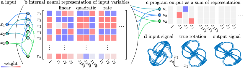
Figure 1: Unfurling neural states as a weighted sum of input variables. (a) Inputs to our RNN, which do not represent specific numerical values, but rather symbolic variables. (b) We expand the activity of the RNN neurons as a weighted sum of polynomials in the input variables and their time derivatives. (c) We can then program an output matrix $W$ that maps the RNN’s symbolic representation of its inputs to any analytical function of the inputs, such as a rotation. (d) When we drive the programmed RNN with a complex input such as the chaotic Thomas attractor, the output indistinguishably rotates the input (typical relative error is less than 1%).

To construct such a language, we begin with a simple equation for our RNN comprising $n$ neurons and $m$ inputs:

$$\frac{1}{\gamma}\dot{\bm{r}}(t)=-\bm{r}(t)+\bm{g}(A\bm{r}(t)+B\bm{x}(t)+\bm{d}).$$ (1)

Here, $\bm{r}\in\mathbb{R}^{n}$ are the neuron states, $\bm{x}\in\mathbb{R}^{m}$ are the input states, $A\in\mathbb{R}^{n\times n}$ are the connections between neurons, $B\in\mathbb{R}^{n\times m}$ are the connections from inputs to neurons, $\bm{d}\in\mathbb{R}^{n}$ are the bias terms, $\bm{g}$ is a sigmoidal function that acts element-wise on its inputs (thereby mapping vectors to vectors), and $\gamma$ is the time constant. In short, Eq. 1 defines the time evolution of neural states as a function of the current neural and input states. For conciseness in what follows, we will omit the notation $(t)$ that explicitly denotes time when obvious.

To define our programming language, we would like to write $\bm{r}$ as a simple function of $\bm{x}$, which is difficult to do for nonlinear systems. Hence, we linearize the system about the neural state $\bm{r}^{*}$, and partially linearize the system about the input state $\bm{x}^{*}$ to yield

$$\frac{1}{\gamma}\dot{\bm{r}}(t)=A^{*}\bm{r}(t)+\bm{u}(\bm{x}(t)),$$ (2)

where $A^{*}$ is the effective dynamical response as $\bm{r}(t)$ deviates slightly away from $\bm{r}^{*}$, and $\bm{u}(\bm{x}(t))$ is the effective input into the system (see Supplemental Section I for the derivation).

Next, because Eq. 2 is linear, we can write the neural states $\bm{r}(t)$ as a convolution of the input with the impulse response. This convolution involving integrals can be expressed algebraically by taking the series expansion of $\bm{u}(\bm{x}(t))$ with respect to time, to yield

$$\begin{split}\bm{r}(t)&=\bm{h}(\bm{x}(t),\dot{\bm{x}}(t),\ddot{\bm{x}}(t),\dotsm),\end{split}$$ (3)

where $\bm{h}$ is an analytic function that we derive in Supplemental Section I. Finally, we perform a Taylor series expansion of $\bm{h}$ with respect to $\bm{x},\dot{\bm{x}},\dotsm$ to decompose the reservoir state $\bm{r}$ as a weighted sum of a polynomial basis of input variables (Fig. 1a,b). It is precisely the coefficients of this expansion—shown in Fig. 1b—that form the start of our recurrent neural programming language. For example, we can program the RNN to output a rotation of its inputs by solving for an output matrix $W\in\mathbb{R}^{k\times 3}$ that rotates any input about the $x_{3}$ axis (Fig. 1c). When we evolve the RNN with the chaotic Thomas attractor given by

$$\begin{split}\dot{x}_{1}(t)&=-3.7x_{1}(t)+5\sin(4x_{2}(t))\\ \dot{x}_{2}(t)&=-3.7x_{2}(t)+5\sin(4x_{3}(t))\\ \dot{x}_{3}(t)&=-3.7x_{3}(t)+5\sin(4x_{1}(t)),\end{split}$$

we find that the output is indistinguishable from a true rotation of the input (Fig. 1d). See Supplemental Section I for a detailed derivation, Supplemental Sections II and III for an explicit quantification of the goodness of the approximation as a function of the RC parameters, and Supplemental Section IV for the parameters used for all examples.

III Natively Distributed and Symbolic Computation

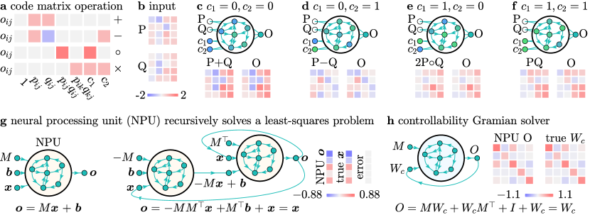
Figure 2: Programming matrix operations and solving equations through feedback. (a) Required code for the RNN output to yield the matrix operations of addition, subtraction, element-wise multiplication, and matrix multiplication at various operating points determined by inputs $c_{1}$ and $c_{2}$. After programming these outputs $o_{ij}$ using a single matrix $W$, we input (b) two matrices P and Q to demonstrate that the output O of the RNN yields the (c) addition, (d) subtraction, (e) element-wise multiplication, and (f) matrix multiplication of P and Q, with indistinguishable error. (g) A neural processing unit (NPU) that outputs the affine transformation of its inputs. By chaining two NPUs, the output is the solution to the least-squares regression problem. Feeding the output back as inputs for $\bm{x}$ solves the least-squares problem, and (h) solves for the controllability Gramian by solving the Lyapunov equation. Typical relative error for all examples is 1% or less.

This programming language defines two fundamentally new computing paradigms. First, it defines a natively symbolic language. As opposed to modern-day silicon computers that are fundamentally numerical and require digitization into binary representations von1993first , many computing tasks—from simple addition to complex matrix multiplication—are most naturally represented with variables. This representational mismatch requires complex algorithms and specialized hardware to numerically implement symbolic operations patterson2016computer . Second, it defines natively distributed processing. As opposed to modern-day silicon computers that must process information sequentially, many computing tasks—from linear regression to matrix equations—are not inherently defined sequentially, but rather through equivalence relations.

We overcome these limitations with our recurrent neural programming language. Specifically, this language is natively symbolic, by which we mean that at the lowest level, neuronal activity is fundamentally a variable function of its inputs. Hence, we can define operations such as matrix addition and multiplication by programming an output matrix $W$ that selects the appropriate terms in the representational basis to form the output $\bm{o}=W\bm{r}$ (Fig. 2a). We can even switch between different symbolic operations by programming our RNN about multiple operating points that we switch between using external inputs $c_{1}$ and $c_{2}$ (Fig. 2b–f).

Using these symbolic outputs, we provide two examples where we further solve symbolic equations in a natively distributed manner using feedback. In the first example, we use a simple neural processing unit (NPU) that is programmed to input a matrix $M$ and two vectors $\bm{b}$ and $\bm{x}$, and to output $\bm{o}=M\bm{x}+\bm{b}$. We chain multiple NPUs to produce more complex expressions—such as the least-squares solution to the linear regression $M\bm{x}=\bm{b}$—as the output. By feeding the output $\bm{o}$ back to drive the $\bm{x}$ inputs, the NPUs converge to the correct solution (Fig. 2g). To understand this convergence, we notice that the output

$$\bm{o}(\bm{x})=-MM^{\top}\bm{x}+M^{\top}\bm{b}+\bm{x}=\bm{x},$$ (4)

is a map from $\bm{x}$ to $\bm{x}$. Through feedback, the RC evolves to the map’s fixed point. In the second example, we calculate the controllability Gramian, $W_{c}$, which is used extensively in many control applications from engineering pasqualetti2014controllability to neuroscience karrer2020practical . To compute $W_{c}$ on a neural computing architecture, we simply program the output to symbolically represent the equation that produces $W_{c}$, and feed the output back into the input for $W_{c}$. By evolving this feedback system, the RNN converges to the correct Gramian (Fig. 2h).

IV Dynamical Random Access Memory

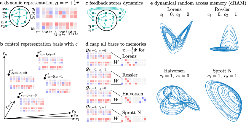
Figure 3: Programming dynamical memories at specific neural addresses. (a) The dynamical representation of an RNN is the series expansion of $\bm{g}(A\bm{r}+B\bm{x}+\bm{d})$. By adding additional control input $c_{1}$ and $c_{2}$, (b) we can evaluate this representation at different equilibrium points of the RNN. (c) To store dynamical memories, we program a single output matrix $W$ that (d) maps each representation to a different dynamical attractor equation $\bm{x}+\frac{1}{\gamma}\dot{\bm{x}}$. (e) By changing the value of $c_{1}$ and $c_{2}$, we can retrieve the dynamical memories in the programmed locations, thereby forming our dynamical random access memory (dRAM).

In addition to defining fundamentally novel and natively symbolic computing paradigms, our recurrent neural programming language extends traditional concepts of computer memory from static to dynamic. Prior work in reservoir computing has demonstrated the power of training RNNs to store dynamical attractors as memories by copying exemplars sussillo2009generating . By dynamical memory, we mean a time series that evolves according to a dynamical equation

$$\dot{\bm{x}}=\bm{f}(\bm{x}).$$

Here we extend such work by programming dynamical memories without any exemplar time series, and by doing so at specific and addressable locations in the RNN’s representation space, thereby yielding a dynamical Random Access Memory (dRAM).

To program dynamical memories, we must first extend our programming language because our current language only defines the RNN state $\bm{r}$ as a function of inputs $\bm{x}$, and encodes nothing about the evolution $\dot{\bm{r}}$ of the RNN. To encode dynamics, we rewrite Eq. 1 as

$$\bm{g}(A\bm{r}+B\bm{x}+\bm{d})=\bm{r}+\frac{1}{\gamma}\dot{\bm{r}}.$$ (5)

We then substitute the expression of $\bm{r}$ as a function of $\bm{x}$ from Eq. 3 to obtain $\bm{g}(A\bm{r}+B\bm{x}+\bm{d})$ as a purely linear combination of polynomial powers of $\bm{x}$ and its time derivatives (Fig. 3a), which yields the final dynamical variant of our programming language. By evaluating Eq. 5 at different constant inputs $c_{1}$ and $c_{2}$, the representational basis also changes (Fig. 3,b).

The program then is a matrix $W$ that simultaneously copies the input state $W\bm{r}=\bm{x}$, and also copies the rate of change of the input state $W\dot{\bm{r}}=\dot{\bm{x}}$ such that

$$W\left(\bm{r}+\frac{1}{\gamma}\dot{\bm{r}}\right)=\bm{x}+\frac{1}{\gamma}\dot{\bm{x}}.$$ (6)

This feedback matrix produces an output $\bm{o}=W\bm{r}$, which—when used in place of the inputs $\bm{x}$ to drive the RC (Fig. 3c)—will store the dynamical memory inside of the RNN. For example, we program $W$ to map the four representational bases generated by setting the control inputs $c_{1}$ and $c_{2}$ to four different dynamical memories (Fig. 3d). Then, depending on the specific value of the control inputs, the output of the RNN yields the four different programmed dynamical memories (Fig. 3e).

V A Recurrent Neural Virtual Machine

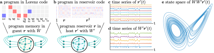
Figure 4: Programming an RNN inside of another RNN. (a) The guest RNN is programmed to store a chaotic Lorenz attractor as a memory using the feedback matrix $W$. The code is $\bm{x}+\frac{1}{\gamma}\dot{\bm{x}}$ according to Eq. 6. (b) The host RNN is programmed to store the guest RNN as a memory using feedback matrix $W^{\prime}$. (c) The host RNN is evolved autonomously forward in time as $\bm{r}^{\prime}(t)$, which (d) simulates the dynamics of the guest RNN as $W^{\prime}\bm{r}^{\prime}(t)$, which (e) simulates the dynamics of the chaotic Lorenz attractor as $WW^{\prime}\bm{r}^{\prime}(t)$.

This ability to store dynamical memories allows us to concretely implement core ideas from computer software into RNNs. Specifically, because an RNN can be programmed to evolve about a dynamical system, and an RNN itself is a dynamical system, we arrive at a curious question: can an RNN be programmed to simulate another RNN? This concept is referred to as a virtual machine rosenblum2005virtual , where a host computer simulates the hardware of a guest computer. We demonstrate that the answer to this question is yes.

First, we program the guest RNN $\bm{r}$ to store a Lorenz attractor as a dynamical memory using a feedback matrix $W$ (Fig. 4a). Then, we write out the code for this programmed guest RNN, and program a separate host RNN $\bm{r}^{\prime}$ to store the programmed guest RNN as a dynamical memory using a feedback matrix $W^{\prime}$ (Fig. 4b). Finally, when we evolve the host RNN (Fig. 4c), we find that it simulates the dynamics of the guest RNN through $W^{\prime}\bm{r}$ (Fig. 4d), which has stored the programmed Lorenz attractor through $WW^{\prime}\bm{r}$ (Fig. 4e).

VI A Logical Calculus Using Recurrent Neural Circuits

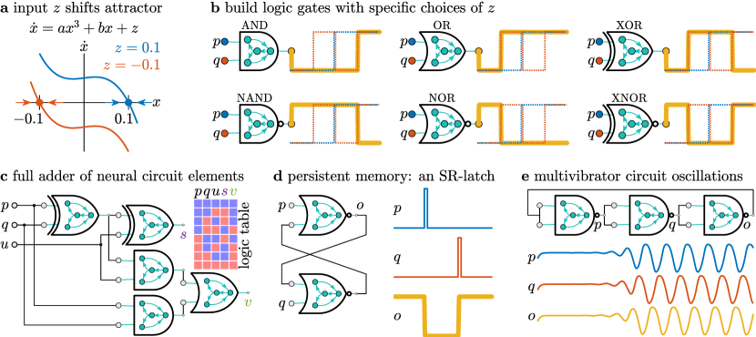
Figure 5: Programming logic gates and circuits using dynamical neural networks. (a) Phase diagram of a cubic dynamical system. When $z=0.1$, the variable $x$ tends towards the stable fixed point $x^{*}=0.1$. When $z=-0.1$, the system bifurcates, and a new stable fixed point emerges at $x^{*}=-0.1$. (b) By setting $z$ equal to various products of two input variables $p$ and $q$, the output evolves according to different Boolean logic gates, and we program these logic gate dynamics into our RNNs. By connecting these neural logic gates, we can form neural circuits that (c) add Boolean numbers, (d) store persistent Boolean states according to a set-reset (SR) latch, and (e) oscillate at a fixed phase difference due to the propagation delay of inversion operations.

This dynamical programming language allows us to greatly expand the computational capability of our RNNs by programming neural implementations of logic gates. While prior work has established the ability of biological and artificial networks to perform computations, here we provide an implementation that makes full use of existing computing frameworks. We program logic gates into distributed RNNs by using a simple dynamical system

$$\dot{x}=ax^{3}+bx+z,$$ (7)

where $a,b,$ and $z$ are parameters. This particular system has the nice property of hysteresis, where when $z=0.1$, the value of $x$ converges to $x=0.1$, but when $z=-0.1$, the value of $x$ jumps discontinuously to converge at $x=-0.1$ (Fig. 5a). This property enables us to program logic gates (Fig. 5b). Specifically, by defining the variable $z$ as a product of two input variables $p$ and $q$, we can program in the dynamics in Eq. 7 to evolve to $-0.1$ or $0.1$ for different patterns of $p$ and $q$.

These logic gates can now take full advantage of existing computing frameworks. For example, we can construct a full adder using neural circuits that take Boolean values $p$ and $q$ as the two numbers to be added, and a “carry” value from the previous addition operation. The adder outputs the sum $s$ and the output carry $v$. We show the inputs and outputs of a fully neural adder in Figure 5c, forming the basis of our ability to program neural logic units (NLU), which are neural analogs of existing arithmetic logic units (ALU).

The emulation of these neural logic gates to circuit design extends even to recurrent circuit architectures. For example, the set-reset (SR) latch—commonly referred to as a flip-flop—is a circuit that holds persistent memory, and is used extensively in computer RAM. We construct a neural SR-latch using two NOR gates with two inputs, $p$ and $q$ (Fig 5d). When $p=0.1$ is pulsed high, the output $o=-0.1$ changes to low. When $q$ is pulsed high, the output changes to high. When both $p$ and $q$ are held low, then the output is fixed at its most recent value (Fig 5d). As another example, we can chain an odd number of inverting gates (i.e., nand, nor, and xor) to construct a multivibrator circuit that generates oscillations (Fig. 5e). Because the output of each gate will be the inverse of its input, if $p$ is high, then $q$ is low, and $o$ is high. However, if we use $o$ as the input to the first gate, then $p$ must switch to low. This discrepancy produces constant fluctuations in the states of $p,q,$ and $o$, which generate oscillations that are offset by the same phase (Fig. 5e).

VII Game Development on Recurrent Neural Architectures

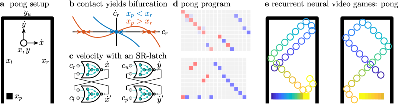
Figure 6: Programming pong using neural circuits and bifurcations. (a) Design of a pong variant. The wall positions ($x_{l},x_{r},y_{u}$) and the paddle’s y-coordinate are fixed as constants. The variables are the ball’s position ($x,y$) and velocity ($\dot{x},\dot{y}$), the paddle’s position ($x_{p}$), and the variables determining contact with the walls and paddle ($c_{l},c_{r},c_{u},c_{p}$). (b) Contact detection with the right wall is implemented using a supercritical pitchfork bifurcation by scaling the $b$ term in Eq. 7 by $x-x_{r}$. When $x<x_{r}$, the contact variable $c_{r}$ goes to 0. When $x>x_{r}$, a bifurcation occurs and $c_{r}$ becomes non-zero. (c) These contact variables are used to drive an SR-latch whose output is the ball’s velocity. (d) Code for the dynamical pong game. (e) An RNN simulating a game of pong in its head. The color from blue to yellow represents the evolution of time. The square on the bottom is the movement of the paddle, and the circle is the movement of the marker.

To demonstrate the flexibility and capacity of our framework, we program a variant of the game “pong” into our RNN as a dynamical system. We begin with the game design by defining the relevant variables and behaviors (Fig. 6a). The variables are the coordinates of the ball, $x,y$, the velocity of the ball, $\dot{x},\dot{y}$, and the position of the paddle, $x_{p}$. Additionally, we have the variables that determine contact with the left, right, and upper walls as $c_{l},c_{r}$, and $c_{u}$, respectively, and the variable that determines contact with the paddle, $c_{p}$. The behavior that we want is for the ball to travel with a constant velocity until it hits either a wall or the paddle, at which point the ball should reverse direction.

Here, we run into our first problem: how do we represent contact detection—a fundamentally discontinuous behavior—using continuous dynamics? Recall that we have already done so to program logic gates in Fig. 5a by using the bifurcation of the cubic dynamical system in Eq. 7. Here, we will use the exact same equation, except rather than changing the parameter $z$ to shift the dynamics up and down (Fig. 5a), we will set the parameter $b$ to skew the shape. As an example, for the right-wall contact $c_{r}$, we will let $b=x-x_{r}$ (Fig. 6b). When the ball is to the left such that $x<x_{r}$, then $c_{r}$ approaches 0. When the ball is to the right such that $x>x_{r}$, then $c_{r}$ becomes non-zero.

To set the velocity of the ball, we use the SR-latch developed in Fig. 5d. When neither wall is in contact, then $c_{r}$ and $c_{l}$ are both low, and the latch’s output does not change. When either the right or the left wall is in contact, then either $c_{r}$ or $c_{l}$ pulses the latch, producing a shift in the velocity (Fig. 6c). Combining these dynamical equations together produces the code for our pong program (Fig. 6d), and the time-evolution of our programmed RNN simulates a game of pong (Fig. 6e).

VIII Discussion

Neural computation exists simultaneously at the core of and the intersection between many fields of study. From the differential binding of neurexins in molecular biology sudhof2017synaptic and neural circuits in neuroscience lerner2016communication ; feller1999spontaneous ; calhoon2015resolving ; maass2007computational ; clarke2013emerging , to the RNNs in dynamical systems sussillo2014neural and neural replicas of computer architectures in machine learning graves2016hybrid , the analogy between neural and silicon computers has generated growing and interdisciplinary interest. Our work provides one possible realization of this analogy by defining a dynamical programming language for RNNs that takes full advantage of their natively continuous and symbolic representation, their parallel and distributed processing, and their dynamical evolution.

This work also makes an important contribution to the increasing interest in alternative computation. A clear example is the vast array of systems—such as molecular kompa2001molecular , DNA zhang2012reversible , and single photon pittman2003experimental —that implement Boolean logic gates. Other examples include the design of materials that compute fang2016pattern ; stern2021supervised and store memories pashine2019directed ; chen2021reprogrammable . Perhaps of most relevance are physical instantiations of reservoir computing in electronic, photonic, mechanical, and biological systems tanaka2019recent . Our work demonstrates the potential of alternative computing frameworks to be fully programmable, thereby shifting paradigms away from imitating silicon computer hardware, and towards defining native programming languages that bring out the full computational capability of each system.

One of the main current limitations is the linear approximation of the RC dynamics. While prior work demonstrates significant computational ability for RCs with largely fluctuating dynamics (i.e., computation at the edge of chaos boedecker2012information ), the approximation used in this work requires that the RC states stay reasonably close to the operating points. While we are able to program a single RC at multiple operating points that are far apart, the linearization is a prominent limitation. Future extensions would use more advanced dynamical approximations into the bilinear regime using Volterra kernels svoronos1980bilinear or Koopman composition operators bevanda2021koopman to better capture nonlinear behaviors.

Finally, we report in the Supplementary Section V an analysis of the gender and racial makeup of the authors we cited in a Citation Diversity Statement.

IX Data & Code Availability Statement

There is no data with mandated deposition used in the manuscript or supplement. All analysis and figures were created programmatically in MATLAB, and the code will be made public upon acceptance of the manuscript.

X Acknowledgments

We gratefully acknowledge Dr. Melody X. Lim, Dr. Kieran A. Murphy, Harang Ju, Dale Zhou, and Dr. Jeni Stiso for conversations and comments on the manuscript. JZK acknowledges support from the National Science Foundation Graduate Research Fellowship No. DGE-1321851. DSB acknowledges support from the John D. and Catherine T. MacArthur Foundation, the ISI Foundation, the Alfred P. Sloan Foundation, an NSF CAREER award PHY-1554488, and from the NSF through the University of Pennsylvania Materials Research Science and Engineering Center (MRSEC) DMR-1720530.

References

- (1) Nieder, A. & Dehaene, S. Representation of number in the brain. Annual review of neuroscience 32, 185–208 (2009).
- (2) Salmelin, R., Hari, R., Lounasmaa, O. V. & Sams, M. Dynamics of brain activation during picture naming. Nature 368, 463–465 (1994).
- (3) Hegarty, M. Mechanical reasoning by mental simulation. Trends in cognitive sciences 8, 280–285 (2004).
- (4) Silver, D. et al. Mastering the game of go with deep neural networks and tree search. nature 529, 484–489 (2016).
- (5) Silver, D. et al. Mastering the game of go without human knowledge. nature 550, 354–359 (2017).
- (6) Patterson, D. A. & Hennessy, J. L. Computer organization and design ARM edition: the hardware software interface (Morgan kaufmann, 2016).
- (7) Von Neumann, J. First draft of a report on the edvac. IEEE Annals of the History of Computing 15, 27–75 (1993).
- (8) Singh, C. & Levy, W. B. A consensus layer v pyramidal neuron can sustain interpulse-interval coding. PloS one 12, e0180839 (2017).
- (9) Gollisch, T. & Meister, M. Rapid neural coding in the retina with relative spike latencies. science 319, 1108–1111 (2008).
- (10) Sigman, M. & Dehaene, S. Brain mechanisms of serial and parallel processing during dual-task performance. Journal of Neuroscience 28, 7585–7598 (2008).
- (11) Nassi, J. J. & Callaway, E. M. Parallel processing strategies of the primate visual system. Nature reviews neuroscience 10, 360–372 (2009).
- (12) Rissman, J. & Wagner, A. D. Distributed representations in memory: insights from functional brain imaging. Annual review of psychology 63, 101–128 (2012).
- (13) Cho, K., Van Merriënboer, B., Bahdanau, D. & Bengio, Y. On the properties of neural machine translation: Encoder-decoder approaches. arXiv preprint arXiv:1409.1259 (2014).
- (14) Towlson, E. K., Vértes, P. E., Ahnert, S. E., Schafer, W. R. & Bullmore, E. T. The rich club of the c. elegans neuronal connectome. Journal of Neuroscience 33, 6380–6387 (2013).
- (15) Werbos, P. J. Backpropagation through time: what it does and how to do it. Proceedings of the IEEE 78, 1550–1560 (1990).
- (16) Caporale, N. & Dan, Y. Spike timing–dependent plasticity: a hebbian learning rule. Annu. Rev. Neurosci. 31, 25–46 (2008).
- (17) Tishby, N., Pereira, F. C. & Bialek, W. The information bottleneck method. arXiv preprint physics/0004057 (2000).
- (18) Olshausen, B. A. & Field, D. J. Emergence of simple-cell receptive field properties by learning a sparse code for natural images. Nature 381, 607–609 (1996).
- (19) Kline, A. G. & Palmer, S. Gaussian information bottleneck and the non-perturbative renormalization group. New Journal of Physics (2021).
- (20) Lukoševičius, M., Jaeger, H. & Schrauwen, B. Reservoir computing trends. KI-Künstliche Intelligenz 26, 365–371 (2012).
- (21) Jaeger, H. The “echo state” approach to analysing and training recurrent neural networks-with an erratum note. Bonn, Germany: German National Research Center for Information Technology GMD Technical Report 148, 13 (2001).
- (22) Sussillo, D. & Abbott, L. F. Generating coherent patterns of activity from chaotic neural networks. Neuron 63, 544–557 (2009).
- (23) Lu, Z., Hunt, B. R. & Ott, E. Attractor reconstruction by machine learning. Chaos: An Interdisciplinary Journal of Nonlinear Science 28, 061104 (2018).
- (24) Kocarev, L. & Parlitz, U. Generalized synchronization, predictability, and equivalence of unidirectionally coupled dynamical systems. Physical review letters 76, 1816 (1996).
- (25) Smith, L. M., Kim, J. Z., Lu, Z. & Bassett, D. S. Learning continuous chaotic attractors with a reservoir computer. Chaos: An Interdisciplinary Journal of Nonlinear Science 32, 011101 (2022).
- (26) Kim, J. Z., Lu, Z., Nozari, E., Pappas, G. J. & Bassett, D. S. Teaching recurrent neural networks to infer global temporal structure from local examples. Nature Machine Intelligence 3, 316–323 (2021).
- (27) Canaday, D., Pomerance, A. & Gauthier, D. J. Model-free control of dynamical systems with deep reservoir computing. Journal of Physics: Complexity 2, 035025 (2021).
- (28) Gauthier, D. J., Bollt, E., Griffith, A. & Barbosa, W. A. Next generation reservoir computing. Nature communications 12, 1–8 (2021).
- (29) Tanaka, G. et al. Recent advances in physical reservoir computing: A review. Neural Networks 115, 100–123 (2019).
- (30) Pasqualetti, F., Zampieri, S. & Bullo, F. Controllability metrics, limitations and algorithms for complex networks. IEEE Transactions on Control of Network Systems 1, 40–52 (2014).
- (31) Karrer, T. M. et al. A practical guide to methodological considerations in the controllability of structural brain networks. Journal of neural engineering 17, 026031 (2020).
- (32) Rosenblum, M. & Garfinkel, T. Virtual machine monitors: Current technology and future trends. Computer 38, 39–47 (2005).
- (33) Südhof, T. C. Synaptic neurexin complexes: a molecular code for the logic of neural circuits. Cell 171, 745–769 (2017).
- (34) Lerner, T. N., Ye, L. & Deisseroth, K. Communication in neural circuits: tools, opportunities, and challenges. Cell 164, 1136–1150 (2016).
- (35) Feller, M. B. Spontaneous correlated activity in developing neural circuits. Neuron 22, 653–656 (1999).
- (36) Calhoon, G. G. & Tye, K. M. Resolving the neural circuits of anxiety. Nature neuroscience 18, 1394–1404 (2015).
- (37) Maass, W., Joshi, P. & Sontag, E. D. Computational aspects of feedback in neural circuits. PLoS computational biology 3, e165 (2007).
- (38) Clarke, L. E. & Barres, B. A. Emerging roles of astrocytes in neural circuit development. Nature Reviews Neuroscience 14, 311–321 (2013).
- (39) Sussillo, D. Neural circuits as computational dynamical systems. Current opinion in neurobiology 25, 156–163 (2014).
- (40) Graves, A. et al. Hybrid computing using a neural network with dynamic external memory. Nature 538, 471–476 (2016).
- (41) Kompa, K. & Levine, R. A molecular logic gate. Proceedings of the National Academy of Sciences 98, 410–414 (2001).
- (42) Zhang, M. & Ye, B.-C. A reversible fluorescent dna logic gate based on graphene oxide and its application for iodide sensing. Chemical Communications 48, 3647–3649 (2012).
- (43) Pittman, T., Fitch, M., Jacobs, B. & Franson, J. Experimental controlled-not logic gate for single photons in the coincidence basis. Physical Review A 68, 032316 (2003).
- (44) Fang, Y., Yashin, V. V., Levitan, S. P. & Balazs, A. C. Pattern recognition with “materials that compute”. Science advances 2, e1601114 (2016).
- (45) Stern, M., Hexner, D., Rocks, J. W. & Liu, A. J. Supervised learning in physical networks: From machine learning to learning machines. Physical Review X 11, 021045 (2021).
- (46) Pashine, N., Hexner, D., Liu, A. J. & Nagel, S. R. Directed aging, memory, and nature’s greed. Science advances 5, eaax4215 (2019).
- (47) Chen, T., Pauly, M. & Reis, P. M. A reprogrammable mechanical metamaterial with stable memory. Nature 589, 386–390 (2021).
- (48) Boedecker, J., Obst, O., Lizier, J. T., Mayer, N. M. & Asada, M. Information processing in echo state networks at the edge of chaos. Theory in Biosciences 131, 205–213 (2012).
- (49) Svoronos, S., Stephanopoulos, G. & Aris, R. Bilinear approximation of general non-linear dynamic systems with linear inputs. International Journal of Control 31, 109–126 (1980).
- (50) Bevanda, P., Sosnowski, S. & Hirche, S. Koopman operator dynamical models: Learning, analysis and control. Annual Reviews in Control 52, 197–212 (2021).