Shfl-BW: Accelerating Deep Neural Network Inference with Tensor-Core Aware Weight Pruning

Abstract.

Weight pruning in deep neural networks (DNNs) can reduce storage and computation cost, but struggles to bring practical speedup to the model inference time. Tensor-cores can significantly boost the throughput of GPUs on dense computation, but exploiting tensor-cores for sparse DNNs is very challenging. Compared to existing CUDA-cores, tensor-cores require higher data reuse and matrix-shaped instruction granularity, both difficult to yield from sparse DNN kernels. Existing pruning approaches fail to balance the demands of accuracy and efficiency: random sparsity preserves the model quality well but prohibits tensor-core acceleration, while highly-structured block-wise sparsity can exploit tensor-cores but suffers from severe accuracy loss.

In this work, we propose a novel sparse pattern, Shuffled Block-wise sparsity (Shfl-BW), designed to efficiently utilize tensor-cores while minimizing the constraints on the weight structure. Our insight is that row- and column-wise permutation provides abundant flexibility for the weight structure, while introduces negligible overheads using our GPU kernel designs. We optimize the GPU kernels for Shfl-BW in linear and convolution layers. Evaluations show that our techniques can achieve the state-of-the-art speed-accuracy trade-offs on GPUs. For example, with small accuracy loss, we can accelerate the computation-intensive layers of Transformer (vaswani2017attention, ) by 1.81, 4.18 and 1.90$\times$ on NVIDIA V100, T4 and A100 GPUs respectively at 75% sparsity.

1. Introduction

Deep neural networks (DNNs) have achieved state-of-the-art results in many domains including speech (amodei2016deep, ), vision (szegedy2015going, ; he2016deep, ) and language (wu2016google, ; vaswani2017attention, ; brown2020language, ). However, DNNs with superior results often have high computation and storage cost. OpenAI summarizes an exponential growth in the operation count and the number of parameters in the state-of-the-art DNN models (openaiblog, ), and many giant language models have recently emerged (brown2020language, ; fedus2021switch, ). Since even the most high-end computing platforms struggle to deploy those advanced models (shoeybi2019megatron, ), their practical adoption is neither technically easy nor economically feasible.

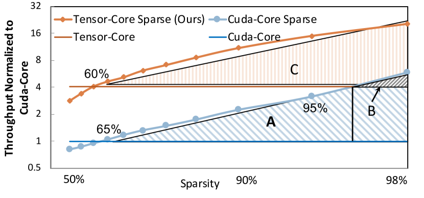
Figure 1. Throughput of Sparse matrix-matrix multiplication (SpMM) compared to dense GEMM. This paper provides the Tensor-Core Sparse curve, which reduces the threshold where sparsity starts to show benefit.

Figure 2. Accuracy-speedup trade-off curve of GNMT model(wu2016google, ) on V100 GPU. Our proposal, Shfl-BW can achieve practical speedup over the tensor-core based dense baseline while unstructured sparsity cannot. Shfl-BW also provides a better trade-off compared to block-wise sparsity.

To turn the algorithmic advances into practical applications, researchers often exploit sparsity for efficient inference, targeting faster execution and less storage. Weight pruning (lecun1990optimal, ; han2015learning, ), which removes unimportant connections in the neural networks, can effectively reduce the operation count and the model size.

Reduced computation, however, does not necessarily lead to speedup. Sparse DNN kernels utilize GPU poorly, due to irregular memory access patterns and lower data reuse than its dense counterparts. On unstructured sparse matrices, the vendor library cuSPARSE (cusparse, ) requires $>98\%$ sparsity to demonstrate practical speedup over the dense baseline on NVIDIA GPUs (Gale2020, ) . With optimizations tailored for DNN’s moderate sparsity, prior arts can only reduce this threshold to around $70\%$ (Gale2020, ).

The tensor cores introduced in recent GPUs significantly boost their computation capabilities, making it more challenging to close the sparse-dense efficiency gap. Fig. 1 shows the throughput of SpMM, which is the kernel inside a weight-pruned linear layer. The shape of GEMM is $M/N/K=2048/128/2048$, and we use Sputnik (Gale2020, ) as the sparse CUDA-core implementation. If both computed with CUDA-cores, SpMM is faster than the dense baseline when the sparsity $>65\%$(region A in Fig. 1). However, CUDA-core based SpMM is less performant than the tensor-core based GEMM until reaching $>95\%$ sparsity (region B). Under such a high sparsity, undesired model accuracy loss is likely to prevent sparse models from being used. This clearly motivates a tensor-core-based sparse DNN solution to justify the performance benefits at a quality-acceptable sparsity-level , which is our focus in this paper(region C).

Unstructured sparsity cannot take good advantages of the tensor-core because it provides little data reuse opportunities and makes sparse kernels memory-bound. Although we can find GPU sparse kernels that manage to use tensor-cores, these kernels have strong requirements on the non-zero structure of sparse matrices, such as a block-wise structure (DeWit2012, ). Such a highly-structured pattern, when used in DNN model pruning, involves high accuracy drop. Balanced sparsity (yao2019balanced, ; cao2019efficient, ), recently supported by the NVIDIA A100 GPU (Nvidia2020, ), is limited by the fixed sparsity level (e.g. only 50% on A100). Moreover, balanced sparsity still faces the memory-bound issue, since redundant data still need to be loaded from DRAM before effective operands are selected out. In summary, towards the goal of tensor-core aware pattern pruning, prior sparsity patterns fail to balance flexibility and computation efficiency. As we will analyze in Section 3, flexibility can be estimated by the number of candidate structures, and computation efficiency can be measured by operation intensity (FLOP-per-byte).

In this paper, we carefully design the sparsity pattern to simultaneously exploit tensor-core acceleration and minimize its constraints on the weight structure. We propose a novel sparsity pattern, Shuffled Block-wise sparsity (Shfl-BW). Fig. 2 shows the advantages of Shfl-BW over other sparsity patterns. Firstly, Shfl-BW can achieve practical speedup over the tensor-core based dense baseline, while unstructured sparsity cannot. Secondly, Shfl-BW dominates block-wise sparsity in computation efficiency-efficiency trade-off.

Shfl-BW is a mutation of the block-wise sparsity with column- and row-wise permutation. The intuition behind Shfl-BW is to preserve the potential data reuse in Block-wise sparsity, but simultaneously enhance the flexibility . Our key insights are two-folds: Firstly, the permutations we apply can asymptotically enlarge the exploration space of weight structure candidates. Secondly, with our GPU kernel designs, the permutation can be performed on-the-fly during the execution of sparse kernels with negligible runtime overheads. Specifically, we handle row-wise permutation with a reordered write-back phase at the end of the kernel, and handle column-wise permutation by stitching input in buffers to construct the same threadblock-scoped tiles as a dense kernel does.

We practice Shfl-BW sparsity on three DNN models, and demonstrate a better accuracy-speedup trade-off than existing pattern pruning methods. Given the recent trend of adding tensor-core-like units in processors to boost DNN workloads (AMD GPU (amd2020cdna, ), Intel CPU (amx, )), we expect our methodology and practice to have wider applications beyond NVIDIA GPUs.

This paper makes the following contributions:

• We propose a novel sparsity pattern, Shuffled Block-wise sparsity (Shfl-BW), that balances flexibility and computation efficiency towards tensor-core aware pattern pruning. Our analysis shows that Shfl-BW enlarges the number of candidate patterns over existing methods (unstructured, block-wise, balanced sparsity), and exposes the same opportunities of data reuse as block-wise and dense kernels.

• On the inference speed side , we implement new GPU kernels for the Shfl-BW pattern to optimize sparse matrix multiplication and convolution layers. Our techniques transform Shfl-BW into Block-wise sparsity during execution on-the-fly with negligible performance overhead.

• On the model accuracy side, we propose heuristic searching methods to prune weights into Shfl-BW structures. Experiments show that models pruned to Shfl-BW sparsity achieves less accuracy loss than the block-wise sparsity.

• Our GPU kernels can accelerate computation-intensive layers in DNN models by up to 1.81, 4.18, 1.90$\times$ on NVIDIA V100, T4 and A100 GPUs at 75% sparsity, respectively. Combined with pruning algorithm, we achieve a new state-of-the-art accuracy-speed trade-off for those popular DNN models.

2. Background and Related Work

2.1. Tensor-Core

The latest NVIDIA Tensor-cores can perform a matrix-multiplication-addition (MMA) of granularity $M/N/K=16/8/16$ in one instruction. The peak throughput of tensor-cores exceeds original CUDA-cores by a large margin, e.g., $4\times$ on V100 and A100 GPU for half precision. Since tensor-cores can effectively accelerate matrix multiplication, they are included in the road-maps of many other processors targeting DNN workloads (e.g. AMD GPUs (amd2020cdna, ) and Intel CPUs (amx, )).

The most computation-intensive operations in many DNN models is General Matrix-Multiplication (GEMM), and when weights are pruned GEMM turns into an SpMM (Sparse-Dense Matrix Product). Tensor cores are very efficient on dense GEMMs, but it is difficult to leverage them in sparse computation, e.g. SpMM. We identify the main challenge is the high demand on data reuse. Since tensor-cores greatly boost the computation throughput but do not change the global bandwidth, it is crucial to increase data reuse, i.e. performing more computation on the loaded values. For example, given the A100 tensor-core throughput and last-level-cache bandwidth  (Nvidia2020, ), one needs to perform $63$ MACs on each loaded value to achieve its peak throughput. SpMM typically exposes much smaller data reuse opportunities, because each value in the dense input matrix is multiplied by fewer values in the other matrix due to sparsity.

2.2. Previous Work

Prior efforts on efficient DNN inference focus on one or more aspects among algorithm, software and hardware. Algorithm-only: early studies explore the opportunities of weight pruning with one-shot pruning (lecun1990optimal, ; han1510compressing, ), and recent studies improve pruning techniques via regularization (zhang2018systematic, ) and weight pattern exploration (ma2021effective, ). This thread of work usually focus on theoretically reducing effective operations in DNN. However, unstructured sparsity can be hard to transform into practical speedup (Figure 1). Software-only (Gale2020, ) and hardware-only (parashar2017scnn, ; han2017ese, ; hegde2019extensor, ) artifacts focus purely on accelerating unstructured sparse kernels in DNN. Instead of trying to accelerate unstructured sparse kernels, the algorithm-hardware co-design approaches propose specialized sparsity patterns that are hardware-friendly, on accelerators (cao2019efficient, ) or GPUs (yao2019balanced, ; Nvidia2020, ). Algorithm-software co-design approaches coordinate pruning pattern and kernel optimizations on GPUs (Guo2020, ) or CPUs (elsen2020fast, ).

Previous studies have proposed many sparsity patterns. Block-wise sparsity requires non-zero weights to form block shapes. An example is the sparse matrix in Figure 3(d), where an entire block of $V\times V$ parameters is either kept or pruned together. An extension of the block-wise sparsity is vector-wise sparsity (Figure 3(c)), i.e. pruning granularity is a $V\times 1$ vector. Balanced sparsity allows $m$ non-zeros within a local shape of $n$ values. For example, the NVIDIA A100 GPU optimizes its tensor-core for the 2-in-4 balanced sparsity: 2 out of consecutive 4 elements in one row are non-zero.

3. The Shfl-BW Sparse Pattern

Figure 3. Different sparse patterns and how to transform from Shfl-BW to block-wise sparsity.

3.1. Shfl-BW Pattern

The key problem in this paper is designing a sparse pattern that balances algorithm and computation need. We need one pattern to efficiently utilize tensor-cores, and at the same time, flexible enough to mimic unstructured sparsity. In existing sparse patterns, these two aspects are hard to coordinate. Figure 3 shows three existing patterns and Shfl-BW, in the descending order of flexibility. The left-most is unstructured sparsity, which sets no pattern constraints at all but are least computation-friendly. Going right, the patterns add more constraints to the weight structure, but the computation efficiency is also improved. Block-wise sparsity is the most computation-friendly, because we can tile it to dense sub-matrices and apply tensor-core based dense kernels on each tile. However, it requires non-zero weights to cluster into blocks and can lead to severe accuracy loss.

Our proposal is Shuffled Block-wise sparsity (Shfl-BW). It enjoys the flexibility of row- and column-wise permutations on top of block-wise sparsity. We manage to recover the computation efficiency through transforming Shfl-BW into block-wise online during kernel execution. Fig. 3 (b) shows an example of Shfl-BW in matrix. At the first look, non-zeros in matrix (b) appear in random positions in the matrix, looking like unstructured sparsity, but they are actually organized by the following rules: through row-wise permutation, we can group together rows with the same non-zero positions, and get a vector-wise sparse matrix with ($V\times 1$) vector shape like matrix (as shown in Figure 3 (c)). Next, through column stitching within each group of $V$ rows, we can get a block-wise sparse matrix with $V\times V$ block shape like matrix (Figure 3 (d)). These two steps not only explain Shfl-BW’s definition, but also are our methods to transform the matrix format from Shfl-BW to block-wise in an SpMM kernel.

3.2. Analysis

3.2.1. Flexibility

To improve the model accuracy under a fixed sparsity, the weight structure should be flexible enough to cover more important weights. We use the number of candidate structures under a certain sparsity to quantify flexibility of a sparse pattern. Shfl-BW performs row shuffling on top of vector-wise sparsity. For the weight matrix of $M$ rows, the candidate space is multiplied by $\frac{M!}{(V!)^{\frac{M}{V}}}$, which is the number of combinations which partition $M$ rows into groups of size $V$. Row-wise shuffling significantly enlarges the candidate space. For example, for a weight matrix with $M=512$ rows and when $V=128$, this combination number already exceeds $e^{700}$.

3.2.2. Computation Efficiency

To increase the utilization of tensor-cores, the weight structure needs to expose the opportunities of data reuse. We evaluate the computation efficiency of a sparse pattern by operation intensity, which equals to dividing the total number of float-point operations by number of bytes loaded from GPU global memory. The data reuse is achieved through tiling. In an SpMM kernel, suppose a GPU threadblock first loads a $T_{M}\times T_{K}$ tile of the left-hand input matrix, and $T_{K}\times T_{N}$ from the right-hand matrix, to the on-chip shared memory. Next, the threadblock multiplies the loaded tiles and accumulate on a $T_{M}\times T_{N}$ output tile stored in the register file. We assume the maximum tiling size as long as the register file is large enough to hold the output accumulators.

We discuss two situations: when the tiled sparse matrix is dense or still sparse. Under unstructured or balanced sparsity, since the non-zeros values are distributed randomly and not forming any dense structures, the tiled sparse matrix is still sparse. We make the tiling size maximum subject to the condition that the register file is large enough to hold the output accumulators. To find out the maximum data reuse is equivalent to solve the following problem:

$${Max\_reuse=}\max_{T_{M},T_{N}}(\frac{2\alpha T_{M}\times T_{N}\times T_{K}\text{Flop}}{\alpha(T_{M}\cdot T_{K})+(T_{K}\cdot T_{N})\cdot 2\text{Byte}}),$$

subject to

$${T_{M}\times T_{N}\leq Size\_regfile}$$

where $\alpha\in(0,1)$ denotes the non-zero ratio. Solving this optimization problem gives us $Max\_reuse=\sqrt{\alpha}Reuse_{dense}$ where $Reuse_{dense}=\frac{T_{opt,dense}}{2}flop/byte$ is the maximum reuse in a dense GEMM, and $T_{opt,dense}=\sqrt{Size\_regfile}$.

On the other hand, under block-wise, vector-wise and our Shfl-BW sparsity, the tiled sparse matrix can be dense. Block-wise matrix is dense within $V\times V$ non-zero blocks, thus if we make $V\times V$ the tiling size, the tiled sparse matrix is dense. The data reuse ratio can reach $Reuse_{dense}$ as long as $V\geq T_{opt,dense}$. Vector-wise and Shfl-BW matrices can be transformed online to block-wise, and achieve the same data reuse ratio.

In summary, in terms of computation efficiency, Shfl-BW, vector-wise and block-wise format exposes higher data reuse opportunities then unstructured and balanced sparsity, because we can tile them into dense sub-matrices. In terms of flexibility, Shfl-BW significantly enlarges the candidate space of block-wise and vector-wise sparsity.

4. GPU Sparse Kernel

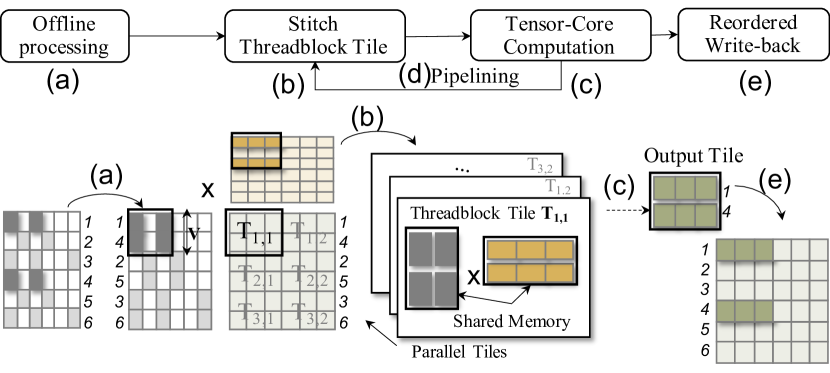
Figure 4. GPU kernel design of Shfl-BW SpMM.

4.1. Overview

Figure 4 shows the key steps in a Shfl-BW GPU SpMM kernel. Step (a) is an offline processing that transforms a Shfl-BW matrix into a vector-wise sparse matrix and an array to store the original row-indices. Storing the sparse matrix in vector-wise format allows us to load values contiguously from the sparse matrix during kernel execution, benefiting the bandwidth efficiency. Step (b) loads tiles of both input matrices into the GPU shared memory. In this step, we perform in-buffer stitching, to be detailed in Section 4.3. Next, in Step (c) we perform matrix-multiplication-addition (MMA) using tensor-cores. Since the loaded tiles are dense, this step is the same as it is in a dense GEMM. We loop over Step (b) and (c) with our pipelining design (marked by (d), detailed in Section 4.4). We point out this kernel requires two-level pre-fetching for sparse metadata and the actual input data, complicating the pipeline schedule. Finally, the output tile is written back to the global memory in Step (e). Because we reorder the sparse matrix rows offline, in this step we perform online reordering and directly write results to the correct rows in the output matrix, to be detailed in Section. 4.2.

The following sections detail our three designs using SpMM as example. We also implement 2D convolutions with similar designs using the implicit-GEMM algorithm (cudnn, ), where the input feature map is unfolded into a matrix form temporally in on-chip buffers.

4.2. Reordered Write-Back

In Figure 4, step (a) and (d) together perform the reordered write-back technique. In Shfl-BW sparse matrix, rows with identical non-zero patterns are scattered to discontiguous positions. For example, in the figure, row $1$ and $4$ have identical patterns. If we compress and store this sparse matrix row-wise, and directly load from these two rows, this uncontiguous memory access pattern cannot fully utilize the global bandwidth. Instead, we reorder Shfl-BW to a vector-wise matrix store weights in the same vector contiguously. We keep the original row-indices in an array for reversing the row order in the output matrix. Steps (b,c,d) perform the SpMM calculation assuming the input is a vector-wise sparse matrix . Finally, when writing the output back to global memory, we refer to the row-indices to directly write in the original row ordering in step (e). We exploit shared memory to buffer the shuffle indices for this tile, so that the number of global memory loads is reduced.

4.3. In-Buffer stitching

Step (b) in Figure 4 illustrates the in-buffer stitching technique. After the offline processing in step (a), the sparse matrix is in vector-wise form. However, tensor-core requires that the reduction dimension in one MMA instruction is at least 8. In order to map to tensor-core granularity, we stitch multiple sparse vectors together. In Figure 4, we stitch two vectors in the sparse matrix to form a $2\times 2$ dense tile just as an example, but in practice the chosen tile size is often $V\times 16$ or larger. When loading the dense matrix, we also stitch data from two discontiguous rows to form a tile. The stitching of the sparse matrix tile is done offline during compression, while the stitching of the dense matrix is done on-the-fly during the loading.

Discussion on the input activation layout: We assume the dense matrices in SpMM has row-major layout, because the memory read/write pattern to the input/output dense matrix are both row-wise. In real models, this means we make batch the innermost dimension of layout in linear layer and 2D convolution. This does not involve transposition overhead in convolution models because convolutions often follow the previous layer’s BatchNorm and is succeeded by another BatchNorm. In models which apply LayerNorm and requires feature to be stored contiguously, transposition is necessary, but transposition can be easily fused into previous LayerNorm and involves negligible overhead (Guo2020, ).

1

Data: A.row_indices[], A.metadata[], A.values[], B[K][N]

Result: C[M][N]

2

3metaload_step = 0;

4 load_step = metaload_step-MetaPrefetchStage;

5 step = load_step - (PipeStage+1);

6 total_step = nnz_this_lane/$T_{K}$;

7 while step ¡ total_step do

8       if metaload_step % MetaPrefetchStage == 0 then

9             BulkLoadMeta(A.metadata[], metaload_step);

10            

11       end if

12      if 0 $\leq$ load_step $\leq$ total_step then

13             StitchTile(buffer[load_step % PipeStage]);

14            

15       end if

16      if step $\geq$ 0 then

17             WarpMMA(buffer[step % PipeStage]);

18            

19       end if

20      step++, load_step++, metaload_step++;

21      

22 end while

23ReorderedWriteBack(C, buffer, A.row_indices[]);

Algorithm 1 GPU SpMM with Shfl-BW sparsity pattern

4.4. Prefetching Meta-Data

Pipelining is an important technique to hide memory loading latency. In SpMM, we not only need to prefetch input tiles (as shown in Line 10 of Algorithm 1), but also the metadata of the sparse weight matrix, which, in our case, is the column indices of the non-zero weights. If we load the metadata and data of the same tile together, it creates an explicit data dependency between the metadata and the activation matrix. This is because during in-buffer stitching, we refer to the column indices to load the relevant rows in the input activation and form the dense matrix tile. To resolve this dependency, we propose to prefetch metadata, i.e. loading metadata of future weight tiles ahead of time. Moreover, metadata usually has a small volume, and aggregating metadata of multiple tiles together leads to more efficient usage of bandwidth. Algorithm 1 shows the pipelining strategy, where metadata is pre-fetched in bulks of $MetaPrefetchStage$ steps (Line 6-8).

5. Pruning Algorithm

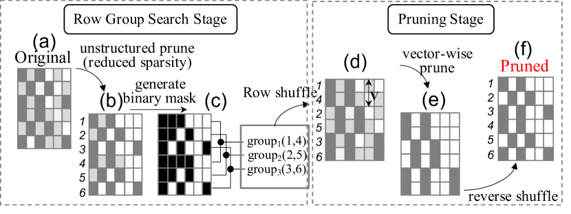
Figure 5. The Shfl-BW pattern searching algorithm.

This section introduces our pruning algorithm for Shfl-BW sparse pattern. Given the importance scores of all weights, our algorithm decides which weights to keep following the Shfl-BW pattern.The Shfl-BW pattern introduces unique challenges to pattern searching due to the enlarged candidate space from row-wise shuffling. In block-wise pattern searching, finding the combination of weight blocks with highest score can be simply done by a greedy method, i.e. selecting blocks with highest scores until the density is reached. However, a greedy method does not work for the Shfl-BW pattern, because selecting a shuffled block implicitly enforcing all the selected weights in these rows to be column-aligned. Formally stated, on an $M\times K$ score matrix , our target is to find a row permutation $\pi$, such that when we shuffle all $M$ rows with $\pi$ and then apply vector-wise pruning, we can obtain the highest total scores. Thus, we design heuristic methods to tackle this search problem.

Figure 5 shows our two-step approach for searching Shfl-BW pattern: firstly, deciding the row shuffling, and secondly, applying vector-wise pruning to the shuffle matrix . The question then becomes how to decide the row shuffling before we are aware of the vector sparse pattern. Observe that after row shuffling, the rows in the same row group will have the same vector column pattern. In other words, they keep the weights in the same columns. The heuristic here is that rows with weights appearing in similar column-wise positions should be reordered together, so that in the next stage, vector-wise pruning will keep more important weights.

The example in Figure 5 elaborates this algorithm. The input to the algorithm is an importance score matrix, as shown in matrix (a). We use the absolute value of each weight as its important score (han2015learning, ). At the first step, we apply unstructured pruning to this score matrix, and keep the $\beta$ weights with highest importance scores. The target non-zero ratio in this step, $\beta$, can be different from the target non-zero ratio of Shfl-BW pruning (denoted as $\alpha$). In practice, we find a reduced sparsity, $\beta=2\alpha$, produces better final results. This unstructured pruning step generates a binary mask as matrix (c), indicating the positions of remained weights. Next, we invoke the K-Means algorithm to cluster the rows in the binary mask into groups with a fixed size, $V$. In this example, each group contains $V=2$ rows. Next, we permute the rows of the original weight matrix to put rows in the same group together and get matrix (d). After reordering the rows, we apply a normal vector-wise pruning to the target non-zero ration $\alpha$ and get the matrix in (e). As the final step, we reverse the row permutation applied to matrix (d), recovering the original row ordering of weights.

6. Evaluation

Figure 6. Speedup against the dense baseline on three GPUs and three models.

6.1. Methodology

Workload: We experiment on three DNN models: Transformer (vaswani2017attention, ) and GNMT (wu2016google, ) on the WMT translation task, and ResNet50 (he2016deep, ) for ImageNet classification. We only calculate the speedup to the linear and 2D convolution layers in the following results. When reporting model kernel speedup, we use the shapes in real model.

Platform: We test on NVIDIA V100, T4 and A100 GPUs, which are the latest three architectures equipped with tensor-cores.

GPU kernel baselines: We compare Shfl-BW with dense, unstructured, block-wise (BW) and vector-wise (VW) sparse patterns. We use cuBLAS (cublas, ) and cuDNN (cudnn, ) as the dense baseline for GEMM and 2D convolution respectively. ‘Unstructured’ baseline comes from Sputnik (Gale2020, ). ‘Balanced‘ sparse kernels is supported by A100 at 50% sparsity only, and we evaluate the SpMM kernel in NVIDIA’s library cuSPARSELt (cusparselt, ). Block-wise baseline comes from NVIDIA cuSPARSE (cusparse, ) library. cuSPARSE does not provide vector-wise kernels, so we implement our own, and in addition we compare with two prior papers on vector-wise kernels: Tilewise (Guo2020, ), which uses CUDA multi-streams, and VectorSparse (Chen2021, ), which is tuned for fine-grained vector-wise SpMM ($V\leq 8$) on tensor-cores.

Pruning settings: We train the GNMT model based on the ADMM (zhang2018systematic, ) method, which improves final accuracy through changing the weight distribution before the pruning step. For Transformer and ResNet50, we apply a newly published workflow named Grow-and-Prune (ma2021effective, ), which improves the quality of pruned model through multiple round of growing and pruning.

6.2. Kernel Speedup

Overall results: Figure 6 shows the speedup over dense kernels for three DNN models, correlated to the sparsity. The baselines all lack implementation for convolution. Tilewise (Guo2020, ) and VectorSparse (Chen2021, ) both need to be compiled on V100 only. $V$ refers to the block (or vector) size in block-wise, vector-wise and Shfl-BW.The throughput of Shfl-BW sparse kernels increase along with sparsity and $V$. For example, on T4 GPU for Transformer GEMM layers, Shfl-BW gives speedup of $3.17/4.18\times$ under $V=32/64$, 75% sparsity, and $3.35/5.04\times$ under $V=32/64$, 85% sparsity. At 75% sparsity, We accelerate the GEMM layers of Transformer (vaswani2017attention, ) by up to 1.81$\times$, 4.18$\times$, 1.90$\times$ on V100, T4 and A100 GPUs respectively. The speedup on T4 is higher than V100 and A100, because T4 has lower ratio of computation capability to bandwidth, posing smaller demand on data reuse.

Comparing sparsity patterns: Unstructured sparsity cannot exceed the dense baseline at even 95% sparsity, because it does not use tensor-cores. Shfl-BW performs comparable to block-wise, while the cuSPARSE block-wise SpMM shows unstable performance across GPUs and block sizes. For example, Shfl-BW is in average 2.88$\times$ cusparse block-wise on T4 GPU at V=64, but only 0.83$\times$ on V100 at $V=32$. Compared to our vector-wise implementation, Shfl-BW is in average $0.97-1.02\times$ faster, showing that row shuffling involves negligible overhead with our reordered write-back technique. Finally, our evaluation shows that on A100, balanced sparsity gives only $1.07\times,1.16\times$ speedup on A100 for Transformer and GNMT, which is less performant than Shfl-BW at $V=64$ at 50% sparsity.

Comparing kernel designs: Our vector-wise and Shfl-BW implementation consistently outperform two vector-wise prior papers. Due to the overhead when the number of streams grows, their multi-stream approach cannot exceed dense baseline under real weight shapes without the neuron pruning applied described in the paper (Guo2020, ) . VectorSparse (Chen2021, ) is less performant than ours because their small vector size ($V=8$) limits data reuse.

		Transformer (BLEU)	GNMT (BLEU)	ResNet50 (Top-1 Acc.%)
80%	BW, V=32	26.92	13.83	75.51
	VW, V=32	26.97	23.1	75.77
	Shfl-BW, V=32	27.23	24.09	76.02
	Shfl-BW, V=64	27.25	23.88	75.94
90%	VW, V=32	26.1	21.27	72.69
	Shfl-BW, V=32	26.29	23.3	73.83
	Shfl-BW, V=64	26.53	22.68	73.09

Table 1. BLEU score and accuracy of pruned models with different sparse patterns.

6.3. Model Accuracy

As shown in Figure 1, at 80% sparsity, Shfl-BW consistently improves the model quality over vector-wise and block-wise. For example on Transformer, Shfl-BW with $V=32$ shows 0.37 drop of BLEU score from the unstructured, but vector-wise at $V=32$ involves 0.63. In most cases, the quality of $V=64$ pruning with shuffling gives better results than a smaller block size but without shuffling.

7. Conclusion

Although tensor-cores significantly increase the throughput of GPUs, it poses challenges on exploiting sparsity for accelerating DNN inference. This paper proposes a new sparsity pattern, Shfl-BW, to strike a better trade-off between flexibility and computation efficiency. We propose GPU sparse kernel designs to exploit tensor-core acceleration. Shfl-BW is comparably efficient but much more flexible than block-wise sparsity. We expect our tensor-core aware pruning methodology to be applicable to a variety of applications, given the emerging trend of adding tensor-core-like units to DNN processors.

References

- [1] Ashish Vaswani et al. Attention is all you need. In Advances in neural information processing systems, pages 5998–6008, 2017.
- [2] Dario Amodei et al. Deep speech 2: End-to-end speech recognition in english and mandarin. In ICML, pages 173–182. PMLR, 2016.
- [3] Christian Szegedy et al. Going deeper with convolutions. In CVPR, pages 1–9, 2015.
- [4] Kaiming He, Xiangyu Zhang, Shaoqing Ren, and Jian Sun. Deep residual learning for image recognition. In CVPR, pages 770–778, 2016.
- [5] Yonghui Wu et al. Google’s neural machine translation system: Bridging the gap between human and machine translation. arXiv preprint arXiv:1609.08144, 2016.
- [6] Tom B Brown et al. Language models are few-shot learners. arXiv preprint arXiv:2005.14165, 2020.
- [7] OpenAI. Ai and compute. https://openai.com/blog/ai-and-compute/.
- [8] William Fedus et al. Switch transformers: Scaling to trillion parameter models with simple and efficient sparsity. arXiv preprint arXiv:2101.03961, 2021.
- [9] Mohammad Shoeybi et al. Megatron-lm: Training multi-billion parameter language models using model parallelism. arXiv preprint arXiv:1909.08053, 2019.
- [10] Yann LeCun et al. Optimal brain damage. In Advances in neural information processing systems, pages 598–605, 1990.
- [11] Song Han et al. Learning both weights and connections for efficient neural networks. arXiv preprint arXiv:1506.02626, 2015.
- [12] NVIDIA. cuSPARSE. https://docs.nvidia.com/cuda/cusparse/index.html.
- [13] Trevor Gale et al. Sparse GPU kernels for deep learning. In SC, pages 1–14. IEEE, 2020.
- [14] S. de Wit et al. GPU kernels for block-sparse weights. Journal of Neuroscience, 32(35):12066–12075, 2012.
- [15] Zhuliang Yao et al. Balanced sparsity for efficient DNN inference on GPU. In AAAI, volume 33, pages 5676–5683, 2019.
- [16] Shijie Cao et al. Efficient and effective sparse LSTM on FPGA with bank-balanced sparsity. In FPGA, pages 63–72, 2019.
- [17] Nvidia. Nvidia A100 tensor core GPU. Data Sheet, pages 20–21, 2020.
- [18] AMD. Introducing the AMD CDNA architecture: the all-new AMD GPU architecture for the modern era of HPC and AI. 2020.
- [19] Intel. Intel architecture instruction set extensions programming reference, 2020.
- [20] Song Han et al. Compressing deep neural networks with pruning, trained quantization and huffman coding. arXiv preprint arXiv:1510.00149, 2015.
- [21] Tianyun Zhang et al. A systematic DNN weight pruning framework using alternating direction method of multipliers. In ECCV, pages 184–199, 2018.
- [22] Xiaolong Ma et al. Effective model sparsification by scheduled grow-and-prune methods. arXiv preprint arXiv:2106.09857, 2021.
- [23] Angshuman Parashar et al. Scnn: An accelerator for compressed-sparse convolutional neural networks. ACM SIGARCH Computer Architecture News, 45(2):27–40, 2017.
- [24] Song Han et al. Ese: Efficient speech recognition engine with sparse LSTM on FPGA. In FPGA, pages 75–84, 2017.
- [25] Kartik Hegde et al. Extensor: An accelerator for sparse tensor algebra. In MICRO, pages 319–333, 2019.
- [26] Cong Guo et al. Accelerating sparse DNN models without hardware-support via tile-wise sparsity. In SC, pages 1–15. IEEE, 2020.
- [27] Erich Elsen et al. Fast sparse convnets. In CVPR, pages 14629–14638, 2020.
- [28] NVIDIA. cuDNN. https://docs.nvidia.com/deeplearning/cudnn/developer-guide/index.html.
- [29] NVIDIA. cuBLAS. https://docs.nvidia.com/cuda/cublas/index.html.
- [30] cusparselt.
- [31] Zhaodong Chen et al. Efficient tensor core-based GPU kernels for structured sparsity under reduced precision. In SC, pages 1–14, 2021.