Data-Efficient Structured Pruning via
Submodular Optimization

Abstract

Structured pruning is an effective approach for compressing large pre-trained neural networks without significantly affecting their performance. However, most current structured pruning methods do not provide any performance guarantees, and often require fine-tuning, which makes them inapplicable in the limited-data regime. We propose a principled data-efficient structured pruning method based on submodular optimization. In particular, for a given layer, we select neurons/channels to prune and corresponding new weights for the next layer, that minimize the change in the next layer’s input induced by pruning. We show that this selection problem is a weakly submodular maximization problem, thus it can be provably approximated using an efficient greedy algorithm. Our method is guaranteed to have an exponentially decreasing error between the original model and the pruned model outputs w.r.t the pruned size, under reasonable assumptions. It is also one of the few methods in the literature that uses only a limited-number of training data and no labels. Our experimental results demonstrate that our method outperforms state-of-the-art methods in the limited-data regime.

1 Introduction

As modern neural networks (NN) grow increasingly large, with some models reaching billions of parameters (McGuffie and Newhouse, 2020), they require an increasingly large amount of memory, power, hardware, and inference time, which makes it necessary to compress them. This is especially important for models deployed on resource-constrained devices like mobile phones and smart speakers, and for latency-critical applications such as self-driving cars.

Several approaches exist to compress NNs. Some methods approximate model weights using quantization and hashing (Gong et al., 2014; Courbariaux et al., 2015), or low-rank approximation and tensor factorization (Denil et al., 2013; Lebedev et al., 2015; Su et al., 2018). In another class of methods called knowledge distillation, a small network is trained to mimic a much larger network (Bucila et al., 2006; Hinton et al., 2015). Other methods employ sparsity and group-sparsity regularisation during training, to induce sparse weights (Collins and Kohli, 2014; Voita et al., 2019).

In this work, we follow the network pruning approach, where the redundant units (weights, neurons or filters/channels) of a pre-trained NN are removed; see (Kuzmin et al., 2019; Blalock et al., 2020; Hoefler et al., 2021) for recent surveys. We also focus on the limited-data regime, where only few training data is available and data labels are unavailable. The advantage of pruning approaches is that, unlike weights approximation-based methods, they preserve the network structure, allowing retraining after compression, and unlike training-based approaches, they do not require training from scratch, which is costly and requires large training data. It is also possible to combine different compression approaches to compound their benefits, see e.g., (Kuzmin et al., 2019, Section 4.3.4).

Existing pruning methods fall into two main categories: unstructured pruning methods which prune individual weights leading to irregular sparsity patterns, and structured pruning methods which prune regular regions of weights, such as neurons, channels, or attention heads. Structured pruning methods are generally preferable as the resulting pruned models can work with off-the-shelf hardware or kernels, as opposed to models pruned with unstructured pruning which require specialized ones.

The majority of existing structured pruning methods are heuristics that do not offer any theoretical guarantees. Moreover, most pruning methods are inapplicable in the limited-data regime, as they rely on fine-tuning with large training data for at least a few epochs to recover some of the accuracy lost with pruning. Mariet and Sra (2015) proposed a “reweighting" procedure applicable to any pruning method, which optimize the remaining weights of the next layer to minimize the change in the input to the next layer. Their empirical results on pruning single linear layers suggest that reweighting can provide a similar boost to performance as fine-tuning, without the need for data labels.

Our contributions

We propose a principled data-efficient structured pruning method based on submodular optimization. In each layer, our method simultaneously selects neurons to prune and new weights for the next layer, that minimize the change in the next layer’s input induced by pruning. The optimization with respect to the weights, for a fixed selection of neurons, is the same one used for reweighting in (Mariet and Sra, 2015). The resulting subset selection problem is intractable, but we show that it can be formulated as a weakly submodular maximization problem (see Definition 2.1). We can thus use the standard greedy algorithm to obtain a $(1-e^{-\gamma})$-approximation to the optimal solution, where $\gamma$ is non-zero if we use sufficient training data. We further adapt our method to prune any regular regions of weights; we focus in particular on pruning channels in convolution layers. To prune multiple layers in the network, we apply our method to each layer independently or sequentially.

We show that the error induced by pruning with our method on the model output decays with an $O(e^{-\gamma k})$ rate w.r.t the number $k$ of neurons/channels kept, under reasonable assumptions. Our method uses only limited training data and no labels. Similar to (Mariet and Sra, 2015), we observe that reweighting provides a significant boost in performance not only to our method, but also to other baselines we consider. However unlike (Mariet and Sra, 2015), we only use a small fraction of the training data, around $\sim$ 1% in our experiments. Our experimental results demonstrate that our method outperforms state-of-the-art pruning methods, even when reweighting is applied to them too, in the limited-data regime, and it is among the best performing methods in the standard setting.

Related work

A large variety of structured pruning approaches has been proposed in the literature, based on different selection schemes and algorithms to solve them. Some works prune neurons/channels individually based on some importance score (He et al., 2014; Li et al., 2017; Liebenwein et al., 2020; Mussay et al., 2020, 2021; Molchanov et al., 2017; Srinivas and Babu, 2015). Such methods are efficient and easy to implement, but they fail to capture higher-order interactions between the pruned parameters. Most do not provide any performance guarantee. One exception are the sampling-based methods of (Liebenwein et al., 2020; Mussay et al., 2020, 2021), who show an $O(1/k)$ error rate, under some assumptions on the model activations.

Closer to our approach are methods that aim to prune neurons/channels that minimize the change induced by pruning in the output of the layer being pruned, or its input to the next layer (Luo et al., 2017; He et al., 2017; Zhuang et al., 2018; Ye et al., 2020b). These criteria yield an intractable combinatorial problem. Existing methods either use a heuristic greedy algorithm to solve it (Luo et al., 2017; Zhuang et al., 2018), or they solve instead its $\ell_{1}$-relaxation using alternating minimization (He et al., 2017), or a greedy algorithm with Frank-Wolfe like updates (Ye et al., 2020b). Among these works only (Ye et al., 2020b) provides theoretical guarantees, showing an $O(e^{-ck})$ error rate. Their method is more expensive than ours, and only optimize the scaling of the next layer weights instead of the weights themselves. A global variant of this method is proposed in Ye et al. (2020a, b), which aim to prune neurons/channels that directly minimize the loss of the pruned network. A similar greedy algorithm with Frank-Wolfe like updates is used to solve the $\ell_{1}$-relaxation of the selection problem. This method has an $O(1/k^{2})$ error rate and is very expensive, as it requires a full forward pass through the network at each iteration. See Appendix A for a more detailed comparison of our method with those of (Ye et al., 2020a, b).

Mariet and Sra (2015) depart from the usual strategy of pruning parameters whose removal influences the network the least. They instead select a subset of diverse neurons to keep in each layer by sampling from a Determinantal Point Process, then they apply their reweighting procedure. Their experimental results show that the advantage of their method is mostly due to reweighting (see Figure 4 therein).

2 Preliminaries

We begin by introducing our notation and some relevant background from submodular optimization.

Notation:

Given a ground set $V=\{1,2,\cdots,d\}$ and a set function $F:2^{V}\to\mathbb{R}_{+}$, we denote the marginal gain of adding a set $I\subseteq V$ to another set $S\subseteq V$ by $F(I\mid S)=F(S\cup I)-F(S)$, which quantifies the change in value when adding $I$ to $S$. The cardinality of a set $S$ is written as $|S|$. Given a vector $x\in\mathbb{R}^{d}$, we denote its support set by $\mathrm{supp}(x)=\{i\in V|x_{i}\not=0\}$, and its $\ell_{2}$-norm by $\|x\|_{2}$. Given a matrix $X\in\mathbb{R}^{d^{\prime}\times d}$, we denote its $i$-th column by $X_{i}$, and its Frobenius norm by $\|X\|_{F}$. Given a set $S\subseteq V$, $X_{S}$ is the matrix with columns $X_{i}$ for all $i\in S$, and $0$ otherwise, and $\boldsymbol{1}_{S}$ is the indicator vector of $S$, with $[\boldsymbol{1}_{S}]_{i}=1$ for all $i\in S$, and $0$ otherwise.

Weakly submodular maximization:

Algorithm 1 Greedy

1:  Input: Ground set $V$, set function $F:2^{V}\to\mathbb{R}_{+}$, budget $k\in\mathbb{N}_{+}$

2:  $S\leftarrow\emptyset$

3:  while $|S|<k$ do

4:     $i^{*}\leftarrow\operatorname*{arg\,max}_{i\in V\setminus S}F(i\mid S)$

5:     $S\leftarrow S\cup\{i^{*}\}$

6:  end while

7:  Output: $S$

A set function $F$ is submodular if it has diminishing marginal gains: $F(i\mid S)\geq F(i\mid T)$ for all $S\subseteq T$, $i\in V\setminus T$. We say that $F$ is normalized if $F(\emptyset)=0$, and non-decreasing if $F(S)\leq F(T)$ for all $S\subseteq T$.
Given a non-decreasing submodular function $F$, selecting a set $S\subseteq V$ with cardinality $|S|\leq k$ that maximize $F(S)$ can be done efficiently using the Greedy algorithm (Alg. 1). The returned solution is guaranteed to satisfy $F(\hat{S})\geq(1-1/e)\max_{|S|\leq k}F(S)$ (Nemhauser et al., 1978). In general though maximizing a non-submodular function over a cardinality constraint is NP-Hard (Natarajan, 1995). However, Das and Kempe (2011) introduced a notion of weak submodularity which is sufficient to obtain a constant factor approximation with the Greedy algorithm.

Definition 2.1.

Given a set function $F:2^{V}\to\mathbb{R}$, $U\subseteq V,k\in\mathbb{N}_{+}$, we say that $F$ is $\gamma_{U,k}$-weakly submodular, with $\gamma_{U,k}>0$ if

$$\gamma_{U,k}F(S|L)\leq\sum_{i\in S}F(i|L),$$

for every two disjoint sets $L,S\subseteq V$, such that $L\subseteq U,|S|\leq k$.

The parameter $\gamma_{U,k}$ is called the submodularity ratio of $F$. It characterizes how close a set function is to being submodular. If $F$ is non-decreasing then $\gamma_{U,k}\in[0,1]$, and $F$ is submodular if and only if $\gamma_{U,k}=1$ for all $U\subseteq V,k\in\mathbb{N}_{+}$. Given a non-decreasing $\gamma_{\hat{S},k}$-weakly submodular function $F$, the Greedy algorithm is guaranteed to return a solution $\hat{S}$ satisfying $F(\hat{S})\geq(1-e^{-\gamma_{\hat{S},k}})\max_{|S|\leq k}F(S)$ (Elenberg et al., 2016; Das and Kempe, 2011). Hence, the closer $F$ is to being submodular, the better is the approximation guarantee.

3 Reweighted input change pruning

In this section, we introduce our approach for pruning neurons in a single layer. Given a large pre-trained NN, $n$ training data samples, and a layer $\ell$ with $n_{\ell}$ neurons, our goal is to select a small number $k$ out of the $n_{\ell}$ neurons to keep, and prune the rest, in a way that influences the network the least. One way to achieve this is by minimizing the change in input to the next layer $\ell+1$, induced by pruning. However, simply throwing away the activations from the dropped neurons is wasteful. Instead, we optimize the weights of the next layer to reconstruct the inputs from the remaining neurons.

Formally, let $A^{\ell}\in\mathbb{R}^{n\times n_{\ell}}$ be the activation matrix of layer $\ell$ with columns $a^{\ell}_{1},\cdots,a^{\ell}_{n_{\ell}}$, where $a^{\ell}_{i}\in\mathbb{R}^{n}$ is the vector of activations of the $i$th neuron in layer $\ell$ for each training input, and let $W^{\ell+1}\in\mathbb{R}^{n_{\ell}\times n_{\ell+1}}$ be the weight matrix of layer $\ell+1$ with columns $w^{\ell+1}_{1},\cdots,w^{\ell+1}_{n_{\ell+1}}$, where $w^{\ell+1}_{i}\in\mathbb{R}^{n_{\ell}}$ is the vector of weights connecting the $i$th neuron in layer $\ell+1$ to the neurons in layer $\ell$. When a neuron is pruned in layer $\ell$, the corresponding column of weights in $W^{\ell}$ and row in $W^{\ell+1}$ are removed. Pruning $n_{\ell}-k$ neurons in layer $\ell$ reduces the number of parameters and computation cost by $(n_{\ell}-k)/n_{\ell}$ for both layer $\ell$ and $\ell+1$.

Let $V_{\ell}=\{1,\cdots,n_{\ell}\}$. Given a set $S\subseteq V_{\ell}$, we denote by $A^{\ell}_{S}$ the matrix with columns $a^{\ell}_{i}$ for all $i\in S$, and $0$ otherwise. That is, $A^{\ell}_{S}$ is the activation matrix of layer $\ell$ after pruning. We choose a set of neurons $S\subseteq V_{\ell}$ to keep and new weights $\tilde{W}^{\ell+1}\in\mathbb{R}^{n_{\ell}\times n_{\ell+1}}$ that minimize:

$$\min_{|S|\leq k,\tilde{W}^{\ell+1}\in\mathbb{R}^{n_{\ell}\times n_{\ell+1}}}\|A^{\ell}W^{\ell+1}-A^{\ell}_{S}\tilde{W}^{\ell+1}\|_{F}^{2}$$ (1)

Note that $A^{\ell}W^{\ell+1}$ are the original inputs of layer $l+1$, and $A^{\ell}_{S}\tilde{W}^{\ell+1}$ are the inputs after pruning and reweighting, i.e., replacing the weights $W^{\ell+1}$ of layer $\ell+1$ with the new weights $\tilde{W}^{\ell+1}$.

3.1 Greedy selection

Solving Problem (1) exactly is NP-Hard (Natarajan, 1995). However, we show below that it can be formulated as a weakly submodular maximization problem, hence it can be efficiently approximated. Let

$$F(S)=\|A^{\ell}W^{\ell+1}\|_{F}^{2}-\min_{\tilde{W}^{\ell+1}}\|A^{\ell}W^{\ell+1}-A^{\ell}_{S}\tilde{W}^{\ell+1}\|_{F}^{2},$$ (2)

then Problem (1) is equivalent to $\max_{|S|\leq k}F(S)$.

Proposition 3.1.

Given $U\subseteq V,k\in\mathbb{N}_{+}$, $F$ is a normalized non-decreasing $\gamma_{U,k}$-weakly submodular function, with

$$\gamma_{U,k}\geq\frac{\min_{\|z\|_{2}=1,\|z\|_{0}\leq|U|+k}\|A^{\ell}z\|_{2}^{2}}{\max_{\|z\|_{2}=1,\|z\|_{0}\leq|U|+1}\|A^{\ell}z\|^{2}_{2}}.$$

The proof of Proposition 3.1 follows by writing $F$ as the sum of $n_{\ell+1}$ sparse linear regression problems $F(S)=\sum_{m=1}^{n_{\ell+1}}\|A^{\ell}w^{\ell+1}_{m}\|^{2}_{2}-\min_{\mathrm{supp}(\tilde{w}_{m})\subseteq S}\|A^{\ell}w^{\ell+1}_{m}-A^{\ell}\tilde{w}_{m}\|^{2}_{2}$, and from the relation established in (Elenberg et al., 2016; Das and Kempe, 2011) between weak submodularity and sparse eigenvalues of the covariance matrix (see Section B.1).

We use the Greedy algorithm to select a set $\hat{S}\subseteq V_{\ell}$ of $k$ neurons to keep in layer $\ell$. As discussed in Section 2, the returned solution is guaranteed to satisfy

$$F(\hat{S})\geq(1-e^{-\gamma_{\hat{S},k}})\max_{|S|\leq k}F(S)$$ (3)

Computing the lower bound on the submodularity ratio $\gamma_{\hat{S},k}$ in Proposition 3.1 is NP-Hard (Das and Kempe, 2011). It is non-zero if any $\min\{2k,n_{\ell}\}$ columns of $A^{\ell}$ are linearly independent. If the number of training data is larger than the number of neurons, i.e., $n>n_{\ell}$, this is likely to be satisfied. We verify that this is indeed the case in our experiments in Appendix E. We also discuss the tightness of the lower bound in Appendix F.

We show in Appendix D that $F$ satisfies an even stronger notion of approximate submodularity than weak submodularity, which implies a better approximation guarantee for Greedy than the one provided in Eq. (3). Though, this requires a stronger assumption: any $k+1$ columns of $A^{\ell}$ should be linearly independent and all rows of $W^{\ell+1}$ should be linearly independent. In particular, we would need that $n_{\ell}\leq n_{\ell+1}$, which is not always satisfied.

In Section 6, we show that the approximation guarantee of Greedy implies an exponentially decreasing bound on the layerwise error, and on the final output error under a mild assumption.

3.2 Reweighting

For a fixed $S\subseteq V_{\ell}$, the reweighted input change $\|A^{\ell}W^{\ell+1}-A^{\ell}_{S}\tilde{W}^{\ell+1}\|_{F}^{2}$ is minimized by setting

$$\tilde{W}^{\ell+1}=x^{S}(A^{\ell})W^{\ell+1},$$ (4)

where $x^{S}(A^{\ell})\in\mathbb{R}^{n_{\ell}\times n_{\ell}}$ is the matrix with columns $x^{S}(a^{\ell}_{j})$ such that

$$x^{S}(a^{\ell}_{j})\in\operatorname*{arg\,min}_{\mathrm{supp}(x)\subseteq S}\|a_{j}^{\ell}-Ax\|_{2}^{2}\text{ for all $j\in V_{\ell}$}.$$ (5)

Note that the new weights are given by $\tilde{w}^{\ell+1}_{im}=w^{\ell+1}_{im}+\sum_{j\not\in S}[x^{S}(A^{\ell})]_{ij}w_{jm}^{\ell+1}$ for all $i\in S$, and $\tilde{w}^{\ell+1}_{im}=0$ for all $i\not\in S,m\in V_{\ell+1}$. Namely, the new weights merge the weights from the dropped neurons into the kept ones. color=red!30, inline] Remove the above observation if we need the space This is the same reweighting procedure introduced in (Mariet and Sra, 2015). But instead of applying it only at the end to the selected neurons $\hat{S}$, it is implicitly done at each iteration of our pruning method, as it is required to evaluate $F$. We discuss next how this can be done efficiently.

3.3 Cost

Each iteration of Greedy requires $O(n_{\ell})$ function evaluations of $F$. Computing $F(S)$ from scratch needs $O(k\cdot(n_{\ell}\cdot n_{\ell+1}+n\cdot(n_{\ell}+n_{\ell+1}))$ time, so a naive implementation of Greedy is too expensive. The following Proposition outlines how we can efficiently evaluate $F(S+i)$ given that $F(S)$ was computed in the previous iteration.

Proposition 3.2.

Given $S\subseteq V_{\ell}$ such that $|S|\leq k$, $i\not\in S$, let $\mathrm{proj}_{S}(a_{j}^{\ell})=A^{\ell}_{S}x^{S}(a_{j}^{\ell})$ be the projection of $a_{j}^{\ell}$ onto the column space of $A^{\ell}_{S}$, $R_{S}(a_{i}^{\ell})=a_{i}^{\ell}-\mathrm{proj}_{S}(a_{i}^{\ell})$ and $\mathrm{proj}_{R_{S}(a_{i}^{\ell})}(a_{j}^{\ell})\in\operatorname*{arg\,min}_{z=R_{S}(a_{i}^{\ell})\gamma,\gamma\in\mathbb{R}}\|a_{j}^{\ell}-z\|_{2}^{2}$ the corresponding residual and the projection of $a_{j}^{\ell}$ onto it. We can write

$$F(i|S)=\sum_{m=1}^{n_{\ell+1}}\|\mathrm{proj}_{R_{S}(a_{i}^{\ell})}(A^{\ell}_{V\setminus S})w_{m}^{\ell+1}\|_{2}^{2},$$

where $\mathrm{proj}_{R_{S}(a_{i})}(A^{\ell}_{V\setminus S})$ is the matrix with columns $\mathrm{proj}_{R_{S}(a_{i})}(a_{j}^{\ell})$ for all $j\not\in S$, $0$ otherwise. Assuming $F(S),\mathrm{proj}_{S}(a_{j}^{\ell})$ and $x^{S}(a_{j}^{\ell})$ for all $j\not\in S$ were computed in the previous iteration, we can compute $F(S+i),\mathrm{proj}_{S+i}(a_{j}^{\ell})$ and $x^{S+i}(a_{j}^{\ell})$ for all $j\not\in(S+i)$ in

$$O(n_{\ell}\cdot(n_{\ell+1}+n+k))\text{ time}.$$

The optimal weights in Eq. (4) can then be computed in $O(k\cdot n_{\ell}\cdot n_{\ell+1})$ time, at the end of Greedy.

The proof is given in Section B.2, and relies on using optimality conditions to construct the least squares solution $x^{S+i}(a_{j}^{\ell})$ from $x^{S}(a_{j}^{\ell})$.
In total Greedy’s runtime is then $O(k\cdot(n_{\ell})^{2}\cdot(n_{\ell+1}+n+k))$. In other words, our pruning method costs as much as $O(k)$ forward passes in layer $\ell+1$ with a batch of size $n$ (assuming $n_{\ell+1}=O(n_{\ell})$). Using a faster variant of Greedy, called Stochastic-Greedy (Mirzasoleiman et al., 2015), further reduces the cost to $O(\log(1/\epsilon)\cdot(n_{\ell})^{2}\cdot(n_{\ell+1}+n+k))$, or equivalently $O(\log(1/\epsilon))$ forward passes in layer $\ell+1$ with a batch of size $n$, while maintaining almost the same approximation guarantee $(1-e^{-\gamma_{\hat{S},k}}-\epsilon)$ in expectation.

Note also that computing the solutions for different budgets $k^{\prime}\leq k$ can be done at the cost of one by running Greedy with budget $k$. Our method is more expensive than methods which prune neurons individually (He et al., 2014; Li et al., 2017; Liebenwein et al., 2020; Mussay et al., 2020, 2021; Molchanov et al., 2017; Srinivas and Babu, 2015), but much less expensive than a loss-based method like (Ye et al., 2020a, b), which requires $O(k)$ forward passes in the full network, for each layer.

4 Pruning regular regions of neurons

In this section, we discuss how to adapt our approach to pruning regular regions of neurons. This is easily achieved by mapping any set of regular regions to the corresponding set of neurons, then applying the same method in Section 3. In particular, we focus on pruning channels in CNNs.

Given a layer $\ell$ with $n_{\ell}$ output channels, let $X^{\ell}\in\mathbb{R}^{n\cdot p_{\ell}\times n_{\ell}\times r_{h}\times r_{w}}$ be its activations for each output channel and training input, where $p_{\ell}$ is number of patches obtained by applying a filter of size $r_{h}\times r_{w}$, and let $F^{\ell+1}\in\mathbb{R}^{n_{\ell+1}\times n_{\ell}\times r_{h}\times r_{w}}$ be the weights of layer $\ell+1$, corresponding to $n_{\ell}$ filters of size $r_{h}\times r_{w}$ for each of its output channels. When an output channel is pruned in layer $\ell$, the corresponding weights in $F^{\ell}$ and $F^{\ell+1}$ are removed. Pruning $n_{\ell}-k$ output channels in layer $\ell$ reduces the number of parameters and computation cost by $(n_{\ell}-k)/n_{\ell}$ for both layer $\ell$ and $\ell+1$. If layer $\ell$ is followed by a batch norm layer, the weights therein corresponding to the pruned channels are also removed.

We arrange the activations $X^{\ell}_{c}\in\mathbb{R}^{n\cdot p_{\ell}\times r_{h}\cdot r_{w}}$ of each channel $c$ into $r_{h}r_{w}$ columns of $A^{\ell}\in\mathbb{R}^{n\cdot p_{\ell}\times n_{\ell}\cdot r_{h}\cdot r_{w}}$, i.e., $A^{\ell}=[X^{\ell}_{1},\cdots,X^{\ell}_{n_{\ell}}]$. Similarly, we arrange the weights $F_{c}^{\ell+1}\in\mathbb{R}^{n_{\ell+1}\times r_{h}\times r_{w}}$ of each channel $c$ into $r_{h}\cdot r_{w}$ rows of $W^{\ell+1}\in\mathbb{R}^{n_{\ell}\cdot r_{h}\cdot r_{w}\times n_{\ell+1}}$, i.e., $(W^{\ell+1})^{\top}=[(F^{\ell}_{1})^{\top},\cdots,(F^{\ell}_{n_{\ell}})^{\top}]$. Recall that $V_{\ell}=\{1,\cdots,n_{\ell}\}$, and let $V^{\prime}_{\ell}=\{1,\cdots,r_{h}r_{w}n_{\ell}\}$. We define a function $M:2^{V_{\ell}}\to 2^{V^{\prime}_{\ell}}$ which maps every channel $c$ to its corresponding $r_{h}r_{w}$ columns in $A^{\ell}$. Let $G(S)=F(M(S))$, with $F$ defined in Eq. (2), then minimizing the reweighted input change $\|A^{\ell}W^{\ell+1}-A^{\ell}_{M(S)}\tilde{W}^{\ell+1}\|_{F}^{2}$ with a budget $k$ is equivalent to $\max_{|S|\leq k}G(S)$. The following proposition shows that this remains a weakly submodular maximization problem.

Proposition 4.1.

Given $U\subseteq V_{\ell},k\in\mathbb{N}_{+}$, $G$ is a normalized non-decreasing $\gamma_{U,k}$-weakly submodular function, with

$$\gamma_{U,k}\geq\frac{\min_{\|z\|_{2}=1,\|z\|_{0}\leq r_{h}r_{w}(|U|+k)}\|A^{\ell}z\|_{2}^{2}}{\max_{\|z\|_{2}=1,\|z\|_{0}\leq r_{h}r_{w}(|U|+1)}\|A^{\ell}z\|^{2}_{2}}.$$

Proof sketch.

$G$ is $\gamma_{U,k}$-weakly submodular iff $F$ satisfies $\gamma_{U,k}F(M(S)|M(L))\leq\sum_{i\in S}F(M(i)|M(L)),$ for every two disjoint sets $L,S\subseteq V_{\ell}$, such that $L\subseteq U,|S|\leq k$. The proof follows by extending the relation established in (Elenberg et al., 2016; Das and Kempe, 2011) between weak submodularity and sparse eigenvalues of the covariance matrix to this case. ∎

As before, we use the Greedy algorithm, with function $G$, to select a set $\hat{S}\subseteq V_{\ell}$ of $k$ channels to keep in layer $\ell$. We get the same approximation guarantee $G(\hat{S})\geq(1-e^{-\gamma_{\hat{S},k}})\max_{|S|\leq k}G(S).$ The submodularity ratio $\gamma_{\hat{S},k}$ is non-zero if any $\min\{2k,n_{\ell}\}r_{h}r_{w}$ columns of $A^{\ell}$ are linearly independent. In our experiments, we observe that in certain layers linear independence only holds for $k$ very small, e.g., $k\leq 0.01n_{\ell}$. This is due to the correlation between patches which overlap. To remedy this, we experimented with using only $r_{h}r_{w}$ random patches from each image, instead of using all patches. This indeed raises the rank of $A^{\ell}$, but certain layers have a very small feature map size so that even the small number of random patches have significant overlap, resulting in still a very small range where linear independence holds, e.g., $k\leq 0.08n_{\ell}$ (see Appendix E for more details). The results obtained with random patches were worst than the ones with all patches, we thus omit them. Note that our lower bounds on $\gamma_{\hat{S},k}$ are not necessarily tight (see Appendix F). Hence, having linear dependence does not necessarily imply that $\gamma_{\hat{S},k}=0$; our method still performs well in these cases.

For a fixed $S\subseteq V_{\ell}$, the optimal weights are again given by $\tilde{W}^{\ell+1}=x^{M(S)}(A^{\ell})W^{\ell+1}$. The cost of running Greedy and reweighting is the same as before (see Section B.2).

5 Pruning multiple layers

In this section, we explain how to apply our pruning method to prune multiple layers of a NN.

5.1 Reweighted input change pruning variants

We consider three variants of our method: LayerInChange, SeqInChange, and AsymInChange. In LayerInChange, we prune each layer independently, i.e., we apply exactly the method in Section 3 or 4, according to the layer’s type. This is the fastest variant; it has the same cost as pruning a single layer, as each layer can be pruned in parallel, and it only requires one forward pass to get the activations of all layers. However, it does not take into account the effect of pruning one layer on subsequent layers.

In SeqInChange, we prune each layer sequentially, starting from the earliest layer to the latest one. For each layer $\ell$, we apply our method with $A^{\ell}$ replaced by the updated activations $B^{\ell}$ after having pruned previous layers, i.e., we solve $\min_{|S|\leq k,\tilde{W}^{\ell+1}\in\mathbb{R}^{n_{\ell}\times n_{\ell+1}}}\|B^{\ell}W^{\ell+1}-B^{\ell}_{S}\tilde{W}^{\ell+1}\|_{F}^{2}$. In AsymInChange, we also prune each layer sequentially, but to avoid the accumulation of error, we use an asymmetric formulation of the reweighted input change, where instead of approximating the updated input $B^{\ell}W^{\ell+1}$, we approximate the original input $A^{\ell}W^{\ell+1}$, i.e., we solve $\min_{|S|\leq k,\tilde{W}^{\ell+1}\in\mathbb{R}^{n_{\ell}\times n_{\ell+1}}}\|A^{\ell}W^{\ell+1}-B^{\ell}_{S}\tilde{W}^{\ell+1}\|_{F}^{2}$. This problem is still a weakly submodular maximization problem, with the same submodularity ratio given in Propositions 3.1 and 4.1, with $A^{\ell}$ replaced by $B^{\ell}$ therein (see Section B.1). Hence, the same approximation guarantee as in the symmetric formulation holds here. Moreover, a better approximation guarantee can again be obtained under stronger assumptions (see Appendix D). The cost of running Greedy with the asymmetric formulation and reweighting is also the same as before (see Section B.2).

In Section 6, we show that the sequential variants of our method both have an exponential error rate, which is faster for the asymmetric variant. We evaluate all three variants in our experiments. As expected, AsymInChange usually performs the best, and LayerInChange the worst.

5.2 Per-layer budget selection

Another important design choice is how much to prune in each layer, given a desired global compression ratio (see Appendix I for the effect of this choice on performance). In our experiments, we use the budget selection method introduced in (Kuzmin et al., 2019, Section 3.4.1), which can be applied to any layerwise pruning method, thus enabling us to have a fair comparison.

Given a network with $L$ layers to prune, let $c=\tfrac{\text{original size}}{\text{pruned size}}$ be the desired compression ratio. We want to select for each layer $\ell$, the number of neurons/channels $k_{\ell}=\alpha_{\ell}n_{\ell}$ to keep, with $\alpha_{\ell}$ chosen from a fixed set of possible values, e.g., $\alpha_{\ell}\in\{0.05,0.1,\cdots,1\}$. We define a layerwise accuracy metric $P_{\ell}(k_{\ell})$ as the accuracy obtained after pruning layer $\ell$, with a budget $k_{\ell}$, while other layers are kept intact, evaluated on a verification set. We set aside a subset of the training set to use as a verification set. Let $P_{\text{orig}}$ be the original model accuracy, $C_{\text{orig}}$ the original model size, and $C(k_{1},\cdots,k_{L})$ the pruned model size. We select the per-layer budgets that minimize the per-layer accuracy drop while satisfying the required compression ratio:

$$\min_{k_{1},\cdots,k_{L}}\{\tau:\forall\ell\in[L],P_{\ell}(k_{\ell})\geq P_{\text{orig}}-\tau,C(k_{1},\cdots,k_{L})\leq C_{\text{orig}}/c\}.$$ (6)

We can solve the selection problem (6) using binary search, if the layerwise accuracy $P_{\ell}(k_{\ell})$ is a non-decreasing function of $k_{\ell}$. Empirically, this is not always the case, the general trend is non-decreasing, but some fluctuations occur. In such cases, we use interpolation to ensure monotonicity.

Alternatively, another simple strategy is to prune each layer until the perlayer error (the reweighted input change in our case) reaches some threshold $\epsilon$, and vary $\epsilon$ to obtain the desired compression ratio, as done in (Zhuang et al., 2018; Ye et al., 2020a).

6 Error convergence rate

In this section, we provide the error rate of our proposed method. The omitted proofs are given in Appendix C. We first show that the change in input to the next layer induced by pruning with our method, with both the symmetric and asymmetric formulation, decays with exponentially fast rate.

Proposition 6.1.

Let $\hat{S}$ be the output of the Greedy algorithm and $\hat{W}^{\ell+1}$ the corresponding optimal weights (Eq. (4)), then

$$\|A^{\ell}W^{\ell+1}-A^{\ell}_{\hat{S}}\hat{W}^{\ell+1}\|_{F}^{2}\leq e^{-\gamma_{\hat{S},n_{\ell}}{k}/{n_{\ell}}}\|A^{\ell}W^{\ell+1}\|_{F}^{2},$$

and

$$\|A^{\ell}W^{\ell+1}-B^{\ell}_{\hat{S}}\hat{W}^{\ell+1}\|_{F}^{2}\leq e^{-\gamma_{\hat{S},n_{\ell}}{k}/{n_{\ell}}}\|A^{\ell}W^{\ell+1}\|_{F}^{2}+(1-e^{-\gamma_{\hat{S},n_{\ell}}{k}/{n_{\ell}}})\min_{\tilde{W}^{\ell+1}\in\mathbb{R}^{n_{\ell}\times n_{\ell+1}}}\|A^{\ell}W^{\ell+1}-B^{\ell}\tilde{W}^{\ell+1}\|_{F}^{2}$$

This follows by extending the approximation guarantee of Greedy in (Elenberg et al., 2016; Das and Kempe, 2011) to $F(\hat{S})\geq(1-e^{-\gamma_{\hat{S},n_{\ell}}{k}/{n_{\ell}}})\max_{|S|\leq n_{\ell}}F(S)$. Note that this bounds uses the submodularity ratio $\gamma_{\hat{S},n_{\ell}}$, for which the lower bound in Proposition 3.1 is non-zero only if all columns of $A^{\ell}$ are linearly independent, which is more restrictive. Though as discussed earlier, this bound is not necessarily tight. We can further extend this exponential layerwise error rate to an exponentially rate on the final output error, if we assume as in (Ye et al., 2020b) that the function corresponding to all layers coming after layer $\ell$ is Lipschitz continuous.

Corollary 6.2.

Let $y\in\mathbb{R}^{n}$ be the original model output, $y^{\hat{S}}\in\mathbb{R}^{n}$ the output after layer $\ell$ is pruned using our method, and $H$ the function corresponding to all layers coming after layer $\ell$, i.e., $y=H(A^{\ell}W^{\ell+1}),y^{\hat{S}}=H(A^{\ell}_{\hat{S}}\hat{W}^{\ell+1})$. If $H$ is Lipschitz continuous with constant $\|H\|_{\text{Lip}}$, then

$$\|y-y^{\hat{S}}\|_{2}^{2}\leq e^{-\gamma_{\hat{S},n_{\ell}}{k}/{n_{\ell}}}\|H\|_{\text{Lip}}^{2}\|A^{\ell}W^{\ell+1}\|_{F}^{2}.$$

Proof.

Since $H$ is Lipschitz continuous, we have $\|y-y^{\hat{S}}\|_{2}^{2}\leq\|H\|_{\text{Lip}}^{2}\|A^{\ell}W^{\ell+1}-A^{\ell}_{\hat{S}}\hat{W}^{\ell+1}\|_{F}^{2}$. The claim then follows from Proposition 6.1. ∎

This matches the exponential convergence rate achieved by the local imitation method in (Ye et al., 2020b, Theorem 1), albeit with a different constant. Under the same assumption, we can show that pruning multiple layers with the sequential variants of our method, SeqInChange and AsymInChange, also admits an exponential convergence rate:

Corollary 6.3.

Let $y\in\mathbb{R}^{n}$ be the original model output, $y^{\hat{S}_{\ell}},{y}^{\tilde{S}_{\ell}}\in\mathbb{R}^{n}$ the outputs after layers $1$ to $\ell$ are sequentially pruned using SeqInChange and AsymInChange, respectively, and $H_{\ell}$ the function corresponding to all (unpruned) layers coming after layer $\ell$. If every function $H_{\ell}$ is Lipschitz continuous with constant $\|H_{\ell}\|_{\text{Lip}}$, then

$$\|y-y^{\hat{S}_{L}}\|_{2}^{2}\leq\sum_{\ell=1}^{L}e^{-\gamma_{\hat{S}_{\ell},n_{\ell}}{k_{\ell}}/{n_{\ell}}}\|H_{\ell}\|_{\text{Lip}}^{2}\|A^{\ell}W^{\ell+1}\|_{F}^{2},$$

and

$$\|y-y^{\tilde{S}_{L}}\|_{2}^{2}\leq\sum_{\ell=1}^{L}\prod_{\ell^{\prime}=\ell+1}^{L}(1-e^{-\gamma_{\tilde{S}_{\ell^{\prime}},n_{\ell^{\prime}}}{k_{\ell^{\prime}}}/{n_{\ell^{\prime}}}})e^{-\gamma_{\tilde{S}_{\ell},n_{\ell}}{k_{\ell}}/{n_{\ell}}}\|H_{\ell}\|_{\text{Lip}}^{2}\|A^{\ell}W^{\ell+1}\|_{F}^{2}.$$

The result is obtained by iteratively applying Proposition 6.1 to the error incurred after each layer is pruned. The rate of SeqInChange matches the exponential convergence rate achieved by the local imitation method in (Ye et al., 2020b, Theorem 6). The bound on AsymInChange is stronger, confirming that the asymmetric formulation indeed reduces the accumulation of errors.

7 Empirical Evaluation

color=red!30, inline] check shrinkbench paper for recommendations for good experimental results In this section, we examine the performance of our proposed pruning method in the limited-data regime. To that end, we focus on one-shot pruning, in which a pre-trained model is compressed in a single step, without any fine-tuning. We study the effect of fine-tuning with both limited and sufficient data in Appendix H. We compare the three variants of our method, LayerInChange, SeqInChange, and AsymInChange, with the following baselines:

• LayerGreedyFS (Ye et al., 2020a): for each layer, first removes all neurons/channels in that layer, then gradually adds back the neuron/channel that yields the largest decrease of the loss, evaluated on one batch of training data. Layers are pruned sequentially from the input to the output layer.

• LayerSampling (Liebenwein et al., 2020): samples neurons/channels, in each layer, with probabilities proportional to sensitivities based on (activations $\times$ weights), and prunes the rest.

• ActGrad (Molchanov et al., 2017): prunes neurons/channels with the lowest (activations $\times$ gradients), averaged over the training data, with layerwise $\ell_{2}$-normalization.

• LayerActGrad: prunes neurons/channels with the lowest (activations $\times$ gradients), averaged over the training data, in each layer. This is the layerwise variant of ActGrad.

• LayerWeightNorm (Li et al., 2017): prunes neurons/channels with the lowest output weights $\ell_{1}$-norm, in each layer.

• Random: prunes randomly selected neurons/channels globally across layers in the network.

• LayerRandom: prunes randomly selected neurons/channels in each layer.

We also considered the global variant of LayerWeightNorm proposed in (He et al., 2014), but we exclude it from plots, as it is always the worst performing method. We evaluate the performance of these methods on the LeNet model (LeCun et al., 1989) on the MNIST dataset (Lecun et al., 1998), and on the ResNet56 (He et al., 2016) and the VGG11 (Simonyan and Zisserman, 2015) models on the CIFAR-10 dataset (Krizhevsky et al., 2009). To ensure a fair comparison, all experiments are based on our own implementation of all the compared methods. To compute the gradients and activations used for pruning in LayerSampling, ActGrad, LayerActGrad, and our method’s variants, we use four batches of $128$ training images, i.e., $n=512$, which corresponds to $\sim 1\%$ of the training data in MNIST and CIFAR10. We consider two variants of the method proposed in (Ye et al., 2020a): a limited-data variant LayerGreedyFS which only uses the same four batches of data used in our method, and a full-data variant LayerGreedyFS-fd with access to the full training data.

We report top-1 accuracy results evaluated on the validation set, as we vary the compression ratio ($\tfrac{\text{original size}}{\text{pruned size}}$). Unless otherwise specified, we use the per-layer budget selection method described in Section 5.2 for all the layerwise pruning methods, except for LayerSampling for which we use its own budget selection strategy provided in (Liebenwein et al., 2020). We use a subset of the training set, of the same size as the validation set, as a verification set for the budget selection method. To disentangle the benefit of using our pruning method from the benefit of reweighting (Section 3.2), we report results with reweighting applied to all pruning methods, or none of them. Though, we will focus our analysis on the more interesting results with reweighting, with the plots without reweighting mostly serving as a demonstration of the benefit of reweighting. Results are averaged over five random runs, with standard deviations plotted as error bars. We report the speedup ($\tfrac{\text{original number of FLOPs}}{\text{pruned number of FLOPs}}$) and pruning time values in Appendix J. For additional details on the experimental set-up, see Appendix G. The code for reproducing all experiments is available at https://github.com/marwash25/subpruning.

LeNet on MNIST

We pre-train LeNet model on MNIST achieving $97.75\%$ top-1 accuracy. We prune all layers except the last classifier layer. Results are presented in Figure 1 (left). All three variants of our method consistently outperform other baselines, even when reweighting is applied to them, with AsymInChange doing the best and LayerInChange the worst. We observe that reweighting significantly improves the performance of all methods except LayerGreedyFS variants.

ResNet56 on CIFAR-10

We use the ResNet56 model pre-trained on CIFAR-10 provided in ShrinkBench (Blalock et al., 2020), which achieves $92.27\%$ top-1 accuracy. We prune all layers except the last layer in each residual branch, the last layer before each residual branch, and the last classifier layer. Results are presented in Figure 1 (middle). The sequential variants of our method perform the best. Their performance is closely matched by LayerWeightNorm and ActGrad (with reweighting) for most compression ratios, except very large ones. LayerInChange performs significantly worst here than the sequential variants of our method. This is likely due to the larger number of layers pruned in ResNet56 compared to LeNet (27 vs 4 layers), which increases the effect of pruning earlier layers on subsequent ones. Here also reweighting improves the performance of all methods except the LayerGreedyFS variants.

VGG11 on CIFAR-10

We pre-train VGG11 model on CIFAR-10 obtaining $90.11\%$ top-1 accuracy. We prune all layers except the last features layer and the last classifier layer. Results are presented in Figure 1 (right). The three variants of our method perform the best. Their performance is matched by ActGrad and LayerWeightNorm (with reweighting). LayerInChange performs similarly to the sequential variants of our method here, even slightly better at compression ratio $32$, probably because the number of layers being pruned is again relatively small (9 layers). As before, reweighting benefits all methods except the LayerGreedyFS variants.

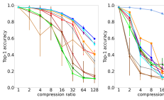
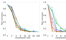
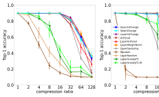
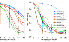
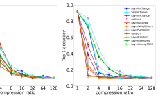
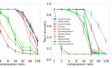
Figure 1: Top-1 Accuracy of different pruning methods applied to LeNet on MNIST (left), ResNet56 on CIFAR10 (middle), and VGG11 on CIFAR10 (right), for several compression ratios (in log-scale), with (top) and without (bottom) reweighting. We include the three reweighted variants of our method in the bottom plots (faded) for reference.

color=red!30, inline] add smthg similar to "We suspect that these favorable properties are explained by the data-informed evaluations of filter importance and the corresponding theoretical guarantees of our algorithm – which enable robustness to variations in network architecture and data distribution."

Discussion

We summarize our observations from the empirical results:

• Our proposed pruning method outperforms state-of-the-art structured pruning methods in various one shot pruning settings. As expected, AsymInChange is the best performing variant of our method, and LayerInChange the worst, with its performance deteriorating with deeper models. Our results also illustrate the robustness of our method, as it reliably yields the best results in various settings, while other baselines perform well in some settings but not in others.

• Reweighting significantly improves performance for all methods, except LayerGreedyFS and LayerGreedyFS-fd. We suspect that reweighting does not help in this case because this method already scales the next layer weights, and it takes into account this scaling when selecting neurons/channels to keep, so replacing it with reweighting can hurt performance.

• The choice of how much to prune in each layer given a global budget can have a drastic effect on performance, as illustrated in Appendix I.

• Fine-tuning with full-training data boosts performance more than reweighting, while fine-tuning with limited data helps less, as illustrated in Appendix H. Reweighting still helps when fine-tuning with limited-data, except for LayerGreedyFS variants, but it can actually deteriorate performance when fine-tuning with full-data. Our method still outperforms other baselines after fine-tuning with limited-data, and is among the best performing methods even in the full-data setting.

color=red!30, inline] time will be highly implementation dependent, and we did not try to optimize our method’s implementation for efficiency. We give theoretical running time which reflect more accurately the computational cost of our method.

8 Conclusion

We proposed a data-efficient structured pruning method, based on submodular optimization. By casting the layerwise subset selection problem as a weakly submodular optimization problem, we are able to use the Greedy algorithm to provably approximate it. Empirically, our method consistently outperforms existing structured pruning methods on different network architectures and datasets.

Checklist

1. For all authors…

   1. Do the main claims made in the abstract and introduction accurately reflect the paper’s contributions and scope? [Yes]

   2. Did you describe the limitations of your work? [Yes] We specify that our focus is on the limited-data regime in both the abstract and introduction. See also the discussions on lines 143-151 and 207-213 on when our approximation guarantee is non-zero, and on lines 173-181 on the cost of our method.

   3. Did you discuss any potential negative societal impacts of your work? [N/A]

   4. Have you read the ethics review guidelines and ensured that your paper conforms to them? [Yes]

2. If you are including theoretical results…

   1. Did you state the full set of assumptions of all theoretical results? [Yes]

   2. Did you include complete proofs of all theoretical results? [Yes] See Appendix B

3. If you ran experiments…

   1. Did you include the code, data, and instructions needed to reproduce the main experimental results (either in the supplemental material or as a URL)? [Yes] We include the code with instructions on how to reproduce all our experimental results in the supplemental material.

   2. Did you specify all the training details (e.g., data splits, hyperparameters, how they were chosen)? [Yes] See Section 7 and Appendix G

   3. Did you report error bars (e.g., with respect to the random seed after running experiments multiple times)? [Yes]

   4. Did you include the total amount of compute and the type of resources used (e.g., type of GPUs, internal cluster, or cloud provider)? [Yes] See Appendix G

4. If you are using existing assets (e.g., code, data, models) or curating/releasing new assets…

   1. If your work uses existing assets, did you cite the creators? [Yes] See Appendix G

   2. Did you mention the license of the assets? [Yes] The license of the assets we used are included in the code we provide.

   3. Did you include any new assets either in the supplemental material or as a URL? [Yes] We include our code in the supplemental material.

   4. Did you discuss whether and how consent was obtained from people whose data you’re using/curating? [N/A]

   5. Did you discuss whether the data you are using/curating contains personally identifiable information or offensive content? [N/A]

5. If you used crowdsourcing or conducted research with human subjects…

   1. Did you include the full text of instructions given to participants and screenshots, if applicable? [N/A]

   2. Did you describe any potential participant risks, with links to Institutional Review Board (IRB) approvals, if applicable? [N/A]

   3. Did you include the estimated hourly wage paid to participants and the total amount spent on participant compensation? [N/A]

Appendix A Additional details on related work

In this section, we give a more detailed comparison of our method with that of [Ye et al., 2020a, b].

Ye et al. [2020a] select neurons/channels to keep in a given layer that minimize the loss of the pruned network. More precisely, they are solving

$$\min_{\alpha\geq 0,\sum_{i}\alpha_{i}=1}\sum_{i=1}^{n}[(f^{\ell}_{\alpha}(x_{i})-y_{i})^{2}],$$

where $(x_{i},y_{i})$ are data points, $f^{\ell}_{\alpha}(x)$ is the output of the model where neurons in layer $\ell$ corresponding to $\alpha_{i}=0$ are pruned and the weights of the next layer are scaled by $\alpha_{i}n_{\ell}$, i.e., $A^{\ell}W^{\ell+1}$ is replaced by $n_{\ell}A^{\ell}\mathrm{Diag}(\alpha)W^{\ell+1}$ where $\mathrm{Diag}(\alpha)$ is the diagonal matrix with $\alpha$ as its diagonal. This is similar to the $\ell_{1}$-relaxation of the selection problem (1) we solve, in the special case of a two layer network with a single output, and instead of optimizing the weights of the next layer like we do, they optimize how much to scale them, i.e., in this case their selection problem reduces to

$$\min_{\alpha\geq 0,\sum_{i}\alpha_{i}=1}\|A^{\ell}w^{\ell+1}-n_{\ell}A^{\ell}\mathrm{Diag}(\alpha)w^{\ell+1}\|_{2}^{2}.$$

They use a greedy algorithm with Frank-Wolfe like updates to approximate it (see [Ye et al., 2020a, Section 12.1] for the relation between their greedy algorithm and Frank-Wolfe algorithm). This method is very expensive as it requires $O(kn_{\ell})$ forward passes in the full network, to prune each layer. The provided theoretical guarantees only holds for two layer networks, and are with respect to an $\ell_{1}$-relaxation of the selection problem. Empirically, our method significantly outperforms the method of [Ye et al., 2020a] in all settings we consider.

Ye et al. [2020b] propose two pruning method: Greedy Global imitation and Greedy Local imitation. Greedy Global imitation is the same method from [Ye et al., 2020a] but with an additional approximation technique which reduces the cost of pruning one layer from $O(kn_{\ell})$ to $O(k)$ forward passes through the full network. This is still more expensive than the cost of our method which is equivalent to $O(1/\epsilon)$ forward passes through only the layer being pruned, if using the fast Greedy algorithm from [Li et al., 2022] (see Section 3.3). Greedy Local imitation is closer to our approach, as it selects neurons/channels to keep in a given layer that minimize the change in the input to the next layer, but it also solves an $\ell_{1}$-relaxation of the selection problem and only optimize the scaling of the next layer weights instead of the weights directly, i.e., it solves

$$\min_{\alpha\geq 0,\sum_{i}\alpha_{i}=1}\|A^{\ell}w^{\ell+1}-n_{\ell}A^{\ell}\mathrm{Diag}(\alpha)w^{\ell+1}\|_{2}^{2}.$$

A similar greedy algorithm with Frank-Wolfe like updates as in [Ye et al., 2020a] is used. Although the selection problem solved is simpler than ours, the cost of pruning one layer is still more expensive than ours: $O(kn_{\ell}n_{\ell+1}n)$ vs $O((n_{\ell})^{2}(n_{\ell+1}+n+k)/\epsilon)$. Ye et al. [2020b] also provide bounds on the difference between the output of the original network and the pruned one, with exponential convergence rate for Greedy Local imitation, and $O(1/k^{2})$ rate for the Greedy Global imitation. Similar guarantees with exponential convergence rate hold for our method (see Section 6). Empirically, the results in [Ye et al., 2020b] show that their global method typically outperforms their local one. So we expect our method to also outperform their local method, since it outperforms their global method.

Appendix B Missing proofs

color=red!30, inline] write the whole appendix for the asymmetric formulation and note that the same properties hold for symmetric formulation by setting $A=B$ and expand on the cases where it makes a difference e.g., for cost. Proofs still need some cleaning up. Recall that $F(S)=\|A^{\ell}W^{\ell+1}\|_{F}^{2}-\min_{\tilde{W}^{\ell+1}\in\mathbb{R}^{n_{\ell}\times n_{\ell+1}}}\|A^{\ell}W^{\ell+1}-A^{\ell}_{S}\tilde{W}^{\ell+1}\|_{F}^{2}$, and $G(S)=F(M(S))$, where $M$ maps each channel to its corresponding columns in $A^{\ell}$. We denote by $\tilde{F}(S)$ the objective corresponding to the asymmetric formulation introduced in Section 5.1, i.e., $\tilde{F}(S)=\|A^{\ell}W^{\ell+1}\|_{F}^{2}-\min_{\tilde{W}^{\ell+1}\in\mathbb{R}^{n_{\ell}\times n_{\ell+1}}}\|A^{\ell}W^{\ell+1}-B^{\ell}_{S}\tilde{W}^{\ell+1}\|_{F}^{2}$, and similarly $\tilde{G}(S)=\tilde{F}(M(S))$, where $M$ maps each channel to its corresponding columns in $A^{\ell}$.

We introduce some notation that will be used throughout the Appendix. Given any matrix $D$ and vector $y$, we denote by $x^{S}(y)\in\operatorname*{arg\,min}_{\mathrm{supp}(x)\subseteq S}\frac{1}{2}\|y-Dx\|_{2}^{2}$ the vector of optimal regression coefficients, and by $\mathrm{proj}_{S}(y)=Dx^{S}(y)$, $R^{S}(y)=y-\mathrm{proj}_{S}(y)$ the corresponding projection and residual.

B.1 Submodularity ratio bounds: Proof of Proposition 3.1 and 4.1 and their extension to the asymmetric formulation

In this section, we prove that $F,G$, and their asymmetric variants $\tilde{F},\tilde{G}$ are all non-decreasing weakly submodular functions. We start by reviewing the definition of restricted smoothness (RSM) and restricted strong convexity(RSC).

Definition B.1 (RSM/RSC).

Given a differentiable function $\ell:\mathbb{R}^{d}\to\mathbb{R}$ and $\Omega\subset\mathbb{R}^{d}\times\mathbb{R}^{d}$, $\ell$ is $\mu_{\Omega}$-RSC and $\nu_{\Omega}$-RSM if $\frac{\mu_{\Omega}}{2}\|x-y\|_{2}^{2}\leq\ell(y)-\ell(x)-\langle\nabla\ell(x),y-x\rangle\leq\frac{\nu_{\Omega}}{2}\|x-y\|_{2}^{2},\;\;\forall(x,y)\in\Omega.$

If $\ell$ is RSC/RSM on $\Omega=\{(x,y):\|x\|_{0}\leq k,\|y\|_{0}\leq k,\|x-y\|_{0}\leq k\}$, we denote by $\mu_{k},\nu_{k}$ the corresponding RSC and RSM parameters.

See 3.1

Proof.

We can write $F(S)=\sum_{m=1}^{n_{\ell+1}}F_{m}(S):=\ell_{m}(0)-\min_{\mathrm{supp}(\tilde{w}_{m})\subseteq S}\ell_{m}(\tilde{w}_{m})$, where $\ell_{m}(\tilde{w}_{m})=\|A^{\ell}w^{\ell+1}_{m}-A^{\ell}\tilde{w}_{m}\|^{2}_{2}$. The function $F_{m}(S)$ is then $\gamma_{U,k}$-weakly submodular with $\gamma_{U,k}\geq\tfrac{\mu_{|U|+k}}{\nu_{|U|+1}}$ [Elenberg et al., 2016], where $\mu_{|U|+k}$ and $\nu_{|U|+1}$ are the RSC and RSM parameters of $\ell_{m}$, given by $\mu_{|U|+k}=\min_{\|z\|_{2}=1,\|z\|_{0}\leq|U|+k}\|A^{\ell}z\|^{2}_{2}$, and $\nu_{|U|+1}=\max_{\|z\|_{2}=1,\|z\|_{0}\leq|U|+1}\|A^{\ell}z\|^{2}_{2}$. It follows then that $F$ is also $\gamma_{U,k}$-weakly submodular. It is easy to check that $F$ is also normalized and non-decreasing. ∎

See 4.1

Proof.

By definition, $G$ is $\gamma_{U,k}$-weakly submodular iff $F$ satisfies

$$\gamma_{U,k}F(M(S)|M(L))\leq\sum_{i\in S}F(M(i)|M(L)),$$

for every two disjoint sets $L,S\subseteq V_{\ell}$, such that $L\subseteq U,|S|\leq k$. We extend the relation established in [Elenberg et al., 2016] between weak submodularity and RSC/RSM parameters to this case.

Let $S^{\prime}=M(S),L^{\prime}=M(L)$, $I^{\prime}=M(i)$, and $k^{\prime}=r_{h}r_{w}k$. As before, we can write $G(S)=F(S^{\prime})=\sum_{m=1}^{n_{\ell+1}}F_{m}(S^{\prime}):=\ell_{m}(0)-\min_{\mathrm{supp}(\tilde{w}_{m})\subseteq S^{\prime}}\ell_{m}(\tilde{w}_{m})$, where $\ell_{m}(\tilde{w}_{m})=\|A^{\ell}w^{\ell+1}_{m}-A^{\ell}\tilde{w}_{m}\|^{2}_{2}$. We denote by $\mu_{k}$ and $\nu_{k}$ the RSC and RSM parameters of $\ell_{m}$, given by $\mu_{k}=\min_{\|z\|_{2}=1,\|z\|_{0}\leq k}\|A^{\ell}z\|^{2}_{2}$, and $\nu_{k}=\max_{\|z\|_{2}=1,\|z\|_{0}\leq k}\|A^{\ell}z\|^{2}_{2}$. To simplify notation, we use $x^{S}:=x^{S}(A^{\ell}w^{\ell+1}_{m})$.

For every two disjoint sets $L,S\subseteq V_{\ell}$, such that $L\subseteq U,|S|\leq k$, we have:

$$0\leq F_{m}(S^{\prime}|L^{\prime}) =\ell_{m}(x^{L^{\prime}})-\ell_{m}(x^{S^{\prime}\cup L^{\prime}})$$

$$\leq-\langle\nabla\ell_{m}(x^{L^{\prime}}),x^{S^{\prime}\cup L^{\prime}}-x^{L^{\prime}}\rangle-\frac{\mu_{|L^{\prime}|+k^{\prime}}}{2}\|x^{S^{\prime}\cup L^{\prime}}-x^{L^{\prime}}\|_{2}^{2}$$

$$\leq\max_{\mathrm{supp}(x)\subseteq S^{\prime}\cup L^{\prime}}-\langle\nabla\ell_{m}(x^{L^{\prime}}),x-x^{L^{\prime}}\rangle-\frac{\mu_{|L^{\prime}|+k^{\prime}}}{2}\|x-x^{L^{\prime}}\|_{2}^{2}$$

By setting $x=x^{L^{\prime}}-\tfrac{[\nabla\ell_{m}(x^{L^{\prime}})]_{S^{\prime}}}{\mu_{|L^{\prime}|+k^{\prime}}}$, we get $G(S^{\prime}|L^{\prime})\leq\frac{\|[\nabla\ell_{m}(x^{L^{\prime}})]_{S^{\prime}}\|_{2}^{2}}{2\mu_{|L^{\prime}|+k^{\prime}}}$.
Given any $i\in S$, $I^{\prime}=M(i)$, we have

$$F_{m}(I^{\prime}|L^{\prime}) =\ell_{m}(x^{L^{\prime}})-\ell_{m}(x^{I^{\prime}\cup L^{\prime}})$$

$$\geq\ell_{m}(x^{L^{\prime}})-\ell_{m}(x^{L^{\prime}}-\frac{[\nabla\ell_{m}(x^{L^{\prime}})]_{I^{\prime}}}{\nu_{|L^{\prime}|+|I^{\prime}|}})$$

$$\geq\langle\nabla\ell_{m}(x^{L^{\prime}}),\frac{[\nabla\ell_{m}(x^{L^{\prime}})]_{I}}{\nu_{|L^{\prime}|+|I^{\prime}|}}\rangle-\frac{\nu_{|L^{\prime}|+k^{\prime}}}{2}\|\frac{[\nabla\ell_{m}(x^{L^{\prime}})]_{I}}{\nu_{|L^{\prime}|+|I^{\prime}|}}\|_{2}^{2}$$

$$=\frac{\|[\nabla\ell_{m}(x^{L^{\prime}})]_{I^{\prime}}\|_{2}^{2}}{2\nu_{|L^{\prime}|+|I^{\prime}|}}$$

Hence,

$$G(S|L)\leq\sum_{m=1}^{n_{\ell+1}}\frac{\|[\nabla\ell_{m}(x^{L^{\prime}})]_{S^{\prime}}\|_{2}^{2}}{2\mu_{|L^{\prime}|+k^{\prime}}} =\sum_{i\in S,I^{\prime}=M(i)}\frac{\|[\nabla\ell_{m}(x^{L^{\prime}})]_{I^{\prime}}\|_{2}^{2}}{2\mu_{|L^{\prime}|+k^{\prime}}}$$

$$=\sum_{i\in S,I^{\prime}=M(i)}\frac{\nu_{|L^{\prime}|+|I^{\prime}|}}{\mu_{|L^{\prime}|+k^{\prime}}}\frac{\|[\nabla\ell_{m}(x^{L^{\prime}})]_{I^{\prime}}\|_{2}^{2}}{2\nu_{|L^{\prime}|+|I^{\prime}|}}=\frac{\nu_{|L^{\prime}|+k^{\prime}}}{\mu_{|L^{\prime}|+k^{\prime}}}\sum_{i\in S}G(i|L).$$

We thus have $\gamma_{U,k}\geq\frac{\mu_{|U^{\prime}|+k^{\prime}}}{\nu_{|U^{\prime}|+|I^{\prime}|}}$. ∎

Both Proposition 3.1 and Proposition 4.1 apply also to the asymmetric variants, using exactly the same proofs.

Proposition B.2.

Given $U\subseteq V,k\in\mathbb{N}_{+}$, $\tilde{F}$ is a normalized non-decreasing $\gamma_{U,k}$-weakly submodular function, with

$$\gamma_{U,k}\geq\frac{\min_{\|z\|_{2}=1,\|z\|_{0}\leq|U|+k}\|B^{\ell}z\|_{2}^{2}}{\max_{\|z\|_{2}=1,\|z\|_{0}\leq|U|+1}\|B^{\ell}z\|^{2}_{2}}.$$

Proposition B.3.

Given $U\subseteq V_{\ell},k\in\mathbb{N}_{+}$, $G$ is a normalized non-decreasing $\gamma_{U,k}$-weakly submodular function, with

$$\gamma_{U,k}\geq\frac{\min_{\|z\|_{2}=1,\|z\|_{0}\leq r_{h}r_{w}(|U|+k)}\|A^{\ell}z\|_{2}^{2}}{\max_{\|z\|_{2}=1,\|z\|_{0}\leq r_{h}r_{w}(|U|+1)}\|A^{\ell}z\|^{2}_{2}}.$$

B.2 Cost bound: Proof of Proposition 3.2 and its extension to other variants

In this section, we investigate the cost of applying Greedy with $F,G$ and their asymmetric variants $\tilde{F},\tilde{G}$. To that end, we need the following key lemmas showing how to update the least squares solutions and the function values after adding one or more elements.

Lemma B.4.

Given a matrix $D$, vector $y$, and a vector of optimal regression coefficients $x^{S}(y)\in\operatorname*{arg\,min}_{\mathrm{supp}(x)\subseteq S}\frac{1}{2}\|y-Dx\|_{2}^{2}$, we have for all $S\subseteq V,i\not\in S$:

$$x^{S\cup i}(y)=(x^{S}(y)-x^{S}(d_{i})\gamma^{S,i}(y))+\gamma^{S,i}(y)\boldsymbol{1}_{i}\in\operatorname*{arg\,min}_{\mathrm{supp}(x)\subseteq S\cup i}\frac{1}{2}\|y-Dx\|_{2}^{2},$$

where $\gamma^{S,i}(y)\in\operatorname*{arg\,min}_{\gamma\in\mathbb{R}}\frac{1}{2}\|y-R^{S}(d_{i})\gamma\|_{2}^{2}$. Hence, $\mathrm{proj}_{S\cup i}(y)=\mathrm{proj}_{S}(y)+\mathrm{proj}_{R^{S}(d_{i})}(y)$, where $\mathrm{proj}_{R^{S}(d_{i})}(y)=R^{S}(d_{i})\gamma^{S,i}(y)$.

Similarly, for $I\subseteq V\setminus S$, let $R^{S}(D_{I})$ be the matrix with columns $R^{S}(d_{i})$, $x^{S}(D_{I})$ the matrix with columns $x^{S}(d_{i})$, and $\gamma^{S,I}(y)\in\operatorname*{arg\,min}_{\gamma\in\mathbb{R}^{|I|}}\frac{1}{2}\|y-R^{S}(D_{I})\gamma\|_{2}^{2}$, then

$$x^{S\cup I}(y)=(x^{S}(y)-x^{S}(D_{I})\gamma^{S,I}(y))+e_{I}\gamma^{S,I}(y)\in\operatorname*{arg\,min}_{\mathrm{supp}(x)\subseteq S\cup I}\frac{1}{2}\|y-Dx\|_{2}^{2},$$

where $e_{I}\in\mathbb{R}^{|V|\times|I|}$ is the matrix with $[e_{I}]_{i,i}=1$ for all $i\in I$, and $0$ elsewhere. Hence, $\mathrm{proj}_{S\cup I}(y)=\mathrm{proj}_{S}(y)+\mathrm{proj}_{R^{S}(D_{I})}(y)$, where $\mathrm{proj}_{R^{S}(D_{I})}(y)=R^{S}(D_{I})\gamma^{S,I}(y)$.

Proof.

By optimality conditions, we have:

$$D_{S}^{\top}(D_{S}x^{S}(y)-y)=0$$ (7)

$$D_{S}^{\top}(D_{S}x^{S}(d_{i})-d_{i})=0\Rightarrow-D_{S}^{\top}R^{S}(d_{i})=0$$ (8)

$$R^{S}(d_{i})^{\top}(R^{S}(d_{i})\gamma^{S,i}(y)-y)=0$$ (9)

We prove that $\hat{x}^{S\cup i}(y)=(x^{S}(y)-x^{S}(d_{i})\gamma^{S,i}(y))+\gamma^{S,i}(y)\boldsymbol{1}_{i}$ satisfies the optimality conditions on $x^{S\cup i}(y)$, hence $\hat{x}^{S\cup i}(y)=x^{S\cup i}(y)$.

We have $D_{S\cup i}\hat{x}^{S\cup i}(y)=D_{S}x^{S}(y)+R^{S}(d_{i})\gamma^{S,i}(y)$, then

$$D_{S}^{\top}(D_{S\cup i}\hat{x}^{S\cup i}(y)-y) =D_{S}^{\top}(D_{S}x^{S}(y)-y)+D_{S}^{\top}R^{S}(d_{i})\gamma^{S,i}(y)=0$$

and

$$d_{i}^{\top}(D_{S\cup i}\hat{x}^{S\cup i}(y)-y) =(R^{S}(d_{i})+D_{S}x^{S}(d_{i}))^{\top}(D_{S}x^{S}(y)+R^{S}(d_{i})\gamma^{S,i}(y)-y)$$

$$=R^{S}(d_{i})^{\top}D_{S}x^{S}(y)+R^{S}(d_{i})^{\top}(R^{S}(d_{i})\gamma^{S,i}(y)-y)$$

$$~{}~{}+(D_{S}x^{S}(d_{i}))^{\top}(D_{S}x^{S}(y)-y)+(D_{S}x^{S}(d_{i}))^{\top}R^{S}(d_{i})\gamma^{S,i}(y)$$

$$=0$$

The proof for the case where we add multiple indices at once follows similarly. ∎

Lemma B.5.

For all $S\subseteq V_{\ell},i\not\in S$, let $R_{S}(b_{i}^{\ell})=b_{i}^{\ell}-\mathrm{proj}_{S}(b_{i}^{\ell})$, $\mathrm{proj}_{R_{S}(b_{i}^{\ell})}(y)=R_{S}(b_{i}^{\ell})\gamma^{S,i}(y)$ with $\gamma^{S,i}(y)\in\operatorname*{arg\,min}_{\gamma\in\mathbb{R}}\|y-R_{S}(b_{i}^{\ell})\gamma\|_{2}^{2}$. We can write the marginal gain of adding $i$ to $S$ w.r.t $\tilde{F}$ as:

$$\tilde{F}(i|S)=\sum_{m=1}^{n_{\ell+1}}\|\mathrm{proj}_{R_{S}(b^{\ell}_{i})}(A^{\ell})w_{m}^{\ell+1}\|_{2}^{2},$$

where $\mathrm{proj}_{R_{S}(b^{\ell}_{i})}(A^{\ell})$ is the matrix with columns $\mathrm{proj}_{R_{S}(b^{\ell}_{i})}(a_{j}^{\ell})$ for all $j\in V_{\ell}$. Similarly, for all $S\subseteq V_{\ell},I\subseteq V_{\ell}\setminus S$, let $R_{S}(B_{I}^{\ell})=B_{I}^{\ell}-\mathrm{proj}_{S}(B_{I}^{\ell})$, $\mathrm{proj}_{R_{S}(B_{I}^{\ell})}(y)=R_{S}(B_{I}^{\ell})\gamma^{S,I}(y)$ with $\gamma^{S,I}(y)\in\operatorname*{arg\,min}_{\gamma\in\mathbb{R}^{|I|}}\|y-R_{S}(B_{I}^{\ell})\gamma\|_{2}^{2}$. We can write the marginal gain of adding $I$ to $S$ w.r.t $\tilde{F}$ as:

$$\tilde{F}(I|S)=\sum_{m=1}^{n_{\ell+1}}\|\mathrm{proj}_{R_{S}(B^{\ell}_{I})}(A^{\ell})w_{m}^{\ell+1}\|_{2}^{2},$$

where $\mathrm{proj}_{R_{S}(B^{\ell}_{I})}(A^{\ell})$ is the matrix with columns $\mathrm{proj}_{R_{S}(B^{\ell}_{I})}(a_{j}^{\ell})$ for all $j\in V_{\ell}$.

Proof.

We prove the claim for the case where we add several elements. The case where we add a single element then follows as a special case. For a fixed $S\subseteq V_{\ell}$, the reweighted asymmetric input change $\|A^{\ell}W^{\ell+1}-B^{\ell}_{S}\tilde{W}^{\ell+1}\|_{F}^{2}$ is minimized by setting $\tilde{W}^{\ell+1}=x^{S}(A^{\ell})W^{\ell+1},$ where $x^{S}(A^{\ell})\in\mathbb{R}^{n_{\ell}\times n_{\ell}}$ is the matrix with columns $x^{S}(a^{\ell}_{j})$ such that

$$x^{S}(a^{\ell}_{j})\in\operatorname*{arg\,min}_{\mathrm{supp}(x)\subseteq S}\|a_{j}^{\ell}-B^{\ell}x\|_{2}^{2}\text{ for all $j\in V_{\ell}$}.$$ (10)

Plugging $\tilde{W}^{\ell+1}$ into the expression of $\tilde{F}(S)$ yields $\tilde{F}(S)=\|A^{\ell}W^{\ell+1}\|_{F}^{2}-\|(A^{\ell}-\mathrm{proj}_{S}(A^{\ell}))W^{\ell+1}\|_{F}^{2},$ where $\mathrm{proj}_{S}(A^{\ell})=B^{\ell}_{S}x^{S}(A^{\ell})$. For every $m\in\{1,\cdots,n_{\ell+1}\}$, we have:

$$\quad\|(\mathrm{proj}_{S\cup I}(A^{\ell})-A^{\ell})w_{m}^{\ell+1}\|_{2}^{2}-\|(\mathrm{proj}_{S}(A^{\ell})-A^{\ell})w_{m}^{\ell+1}\|_{2}^{2}$$

$$=\|(\mathrm{proj}_{S}(A^{\ell})+\mathrm{proj}_{R_{S}(B_{I})}(A^{\ell})-A^{\ell})w_{m}^{\ell+1}\|_{2}^{2}-\|(\mathrm{proj}_{S}(A^{\ell})-A^{\ell})w_{m}^{\ell+1}\|_{2}^{2}$$ (by Lemma B.4)

$$=\|\mathrm{proj}_{R_{S}(B_{I})}(A^{\ell})w_{m}^{\ell+1}\|_{2}^{2}-2\langle(A^{\ell}-\mathrm{proj}_{S}(A^{\ell}))w_{m}^{\ell+1},\mathrm{proj}_{R_{S}(B_{I})}(A^{\ell})w_{m}^{\ell+1}\rangle$$

$$=\|\mathrm{proj}_{R_{S}(B_{I})}(A^{\ell})w_{m}^{\ell+1}\|_{2}^{2}-2\langle\mathrm{proj}_{R_{S}(B_{I})}(A^{\ell})w_{m}^{\ell+1},\mathrm{proj}_{R_{S}(B_{I})}(A^{\ell})w_{m}^{\ell+1}\rangle$$

$$=-\|\mathrm{proj}_{R_{S}(B_{I})}(A^{\ell})w_{m}^{\ell+1}\|_{2}^{2}$$

where the second to last equality holds because $y-\mathrm{proj}_{S}(y)-\mathrm{proj}_{R_{S}(B_{I})}(y)$ and $\mathrm{proj}_{R_{S}(B_{I})}(y^{\prime})$ are orthogonal by optimality conditions (see proof of Lemma B.4):

$$\langle y-\mathrm{proj}_{S}(y)-\mathrm{proj}_{R_{S}(B_{I})}(y),\mathrm{proj}_{R_{S}(B_{I})}(y^{\prime})\rangle=\langle y-B_{S}x^{S}(y)-R_{S}(B_{I})\gamma^{S,I}(y),R_{S}(B_{I})\gamma^{S,I}(y^{\prime})\rangle=0.$$

Hence, $\tilde{F}(I|S)=\sum_{m=1}^{n_{\ell+1}}\|\mathrm{proj}_{R_{S}(B_{I})}(A^{\ell})w_{m}^{\ell+1}\|_{2}^{2}$. In particular, if $I=\{i\}$, $\tilde{F}(i|S)=\sum_{m=1}^{n_{\ell+1}}\|\mathrm{proj}_{R_{S}(b^{\ell}_{i})}(A^{\ell})w_{m}^{\ell+1}\|_{2}^{2}$. ∎

Lemma B.6.

For all $S\subseteq V_{\ell},i\not\in S$, let $R_{S}(a_{i}^{\ell})=a_{i}^{\ell}-\mathrm{proj}_{S}(a_{i}^{\ell})$, $\mathrm{proj}_{R_{S}(a_{i}^{\ell})}(y)=R_{S}(a_{i}^{\ell})\gamma^{S,i}(y)$ with $\gamma^{S,i}(y)\in\operatorname*{arg\,min}_{\gamma\in\mathbb{R}}\|y-R_{S}(a_{i}^{\ell})\gamma\|_{2}^{2}$. We can write the marginal gain of adding $i$ to $S$ w.r.t $F$ as:

$$F(i|S)=\sum_{m=1}^{n_{\ell+1}}\|\mathrm{proj}_{R_{S}(a^{\ell}_{i})}(A^{\ell}_{V\setminus S})w_{m}^{\ell+1}\|_{2}^{2},$$

where $\mathrm{proj}_{R_{S}(a^{\ell}_{i})}(A^{\ell}_{V\setminus S})$ is the matrix with columns $\mathrm{proj}_{R_{S}(a^{\ell}_{i})}(a_{j}^{\ell})$ for all $j\in V\setminus S$, $0$ otherwise. Similarly, for all $S\subseteq V_{\ell},I\subseteq V_{\ell}\setminus S$, let $R_{S}(A_{I}^{\ell})=A_{I}^{\ell}-\mathrm{proj}_{S}(A_{I}^{\ell})$, $\mathrm{proj}_{R_{S}(A_{I}^{\ell})}(y)=R_{S}(A_{I}^{\ell})\gamma^{S,I}(y)$ with $\gamma^{S,I}(y)\in\operatorname*{arg\,min}_{\gamma\in\mathbb{R}^{|I|}}\|y-R_{S}(A_{I}^{\ell})\gamma\|_{2}^{2}$. We can write the marginal gain of adding $I$ to $S$ w.r.t $F$ as:

$$F(I|S)=\sum_{m=1}^{n_{\ell+1}}\|\mathrm{proj}_{R_{S}(A^{\ell}_{I})}(A^{\ell}_{V\setminus S})w_{m}^{\ell+1}\|_{2}^{2},$$

where $\mathrm{proj}_{R_{S}(A^{\ell}_{I})}(A^{\ell}_{V\setminus S})$ is the matrix with columns $\mathrm{proj}_{R_{S}(A^{\ell}_{I})}(a_{j}^{\ell})$ for all $j\in V\setminus S$, $0$ otherwise.

Proof.

Setting $B^{\ell}=A^{\ell}$ in Lemma B.5, we get $F(I|S)=\sum_{m=1}^{n_{\ell+1}}\|\mathrm{proj}_{R_{S}(A^{\ell}_{I})}(A^{\ell})w_{m}^{\ell+1}\|_{2}^{2}$. Note that for all $i\in I,j\in S$, $a_{j}^{\ell}$ and $R_{S}(a_{i}^{\ell})$ are orthogonal, and hence $\mathrm{proj}_{R_{S}(A_{I}^{\ell})}(a_{j}^{\ell})=0$, by optimality conditions (see proof of Lemma B.4). It follows then that $F(I|S)=\sum_{m=1}^{n_{\ell+1}}\|\mathrm{proj}_{R_{S}(A^{\ell}_{I})}(A^{\ell}_{V\setminus S})w_{m}^{\ell+1}\|_{2}^{2}$. In particular, if $I=\{i\}$, $F(i|S)=\sum_{m=1}^{n_{\ell+1}}\|\mathrm{proj}_{R_{S}(a^{\ell}_{i})}(A^{\ell}_{V\setminus S})w_{m}^{\ell+1}\|_{2}^{2}$. ∎

Proposition B.7.

Given $S\subseteq V_{\ell}$ such that $|S|\leq k$, $i\not\in S$, let $\mathrm{proj}_{S}(a_{j}^{\ell})=A^{\ell}_{S}x^{S}(a_{j}^{\ell})$. Assuming $\tilde{F}(S),\mathrm{proj}_{S}(b_{j}^{\ell}),x^{S}(b_{j}^{\ell})$ for all $j\not\in S$, and $x^{S}(a^{\ell}_{j})$ for all $j\in V_{\ell}$, were computed in the previous iteration, we can compute $\tilde{F}(S+i),\mathrm{proj}_{S+i}(b_{j}^{\ell}),x^{S+i}(b_{j}^{\ell})$ for all $j\not\in(S+i)$, and $x^{S+i}(a^{\ell}_{j})$ for all $j\in V_{\ell}$, in

$$O(n_{\ell}\cdot(n_{\ell+1}+n+k))\text{ time}.$$

Computing the optimal weights in Eq. (4) at the end of Greedy can then be done in $O(k\cdot n_{\ell}\cdot n_{\ell+1})$ time.

Proof.

By Lemma B.5, we can update the function value using

$$\tilde{F}(i|S)=\sum_{m=1}^{n_{\ell+1}}\|\mathrm{proj}_{R_{S}(b_{i}^{\ell})}(A^{\ell})w_{m}^{\ell+1}\|_{2}^{2}=\sum_{m=1}^{n_{\ell+1}}(\sum_{j\in V_{\ell}}\gamma^{S,i}(a^{\ell}_{j})w_{jm}^{\ell+1}\big{)}^{2}\|R_{S}(b_{i}^{\ell})\|_{2}^{2}.$$

This requires $O(n)$ to compute $R_{S}(b_{i}^{\ell})$ and its norm, $O(n_{\ell}\cdot n)$ to compute $\gamma^{S,i}(a^{\ell}_{j})=\tfrac{R_{S}(b_{i}^{\ell})^{\top}a^{\ell}_{j}}{\|R_{S}(b_{i}^{\ell})\|_{2}^{2}}$ for all $j\in V_{\ell}$, and an additional $O(n_{\ell}\cdot n_{\ell+1})$ to finally evaluate $\tilde{F}(S+i)$. We also need $O(|S^{c}|\cdot n)$ to update $\mathrm{proj}_{S\cup i}(b_{j})=\mathrm{proj}_{S}(b_{j})+\mathrm{proj}_{R_{S}(b_{i}^{\ell})}(b_{j})$ (by Lemma B.4), using $\mathrm{proj}_{R_{S}(b_{i}^{\ell})}(b_{j})=R_{S}(b_{i}^{\ell})\gamma^{S,i}(b^{\ell}_{j})$ for all $j\in V_{\ell}\setminus S\cup i$, $O(|S^{c}|\cdot|S|)$ to update $x^{S\cup i}(b^{\ell}_{j})=x^{S}(b^{\ell}_{j})+(\boldsymbol{1}_{i}-x^{S}(b_{i}))\gamma^{S,i}(b^{\ell}_{j}))$ (by Lemma B.4) for all $j\in V_{\ell}\setminus S\cup i$, and $O(n_{\ell}\cdot|S|)$ to update $x^{S\cup i}(a^{\ell}_{j})=x^{S}(a^{\ell}_{j})+(\boldsymbol{1}_{i}-x^{S}(b_{i}))\gamma^{S,i}(a^{\ell}_{j}))$ for all $j\in V_{\ell}$. So in total, we need $O(n_{\ell}\cdot(n_{\ell+1}+n+k)).$ Computing the new weights $\tilde{W}^{\ell+1}=x^{S}(A^{\ell})W^{\ell+1}$ at the end can be done in $O(n_{\ell}\cdot n_{\ell+1}\cdot|S|)=O(n_{\ell}\cdot n_{\ell+1}\cdot k)$. ∎

See 3.2

Proof.

The proof follows from Lemma B.6 and B.4 in the same way as in Proposition B.7. ∎

Proposition 3.2 and Proposition B.7 apply also to $G$ and $\tilde{G}$ respectively, since $|M(i)|=O(1)$.

B.3 Extension of Stochastic-Greedy to weakly submodular functions

In this section, we show that the guarantee of Stochastic-Greedy (Algorithm 2) easily extends to weakly submodular functions.

Algorithm 2 Stochastic-Greedy

1:  Input: Ground set $V$, set function $F:2^{V}\to\mathbb{R}_{+}$, budget $k\in\mathbb{N}_{+}$

2:  $S\leftarrow\emptyset$

3:  while $|S|<k$ do

4:     $R\leftarrow$ a random subset obtained by sampling $s$ random elements from $V\setminus S$.

5:     $i^{*}\leftarrow\operatorname*{arg\,max}_{i\in R}F(i\mid S)$

6:     $S\leftarrow S\cup\{i^{*}\}$

7:  end while

8:  Output: $S$

Proposition B.8.

Let $\hat{S}$ be the solution returned by Stochastic-Greedy with $s=\tfrac{n}{k}\log(\tfrac{1}{\epsilon})$, and let $F$ be a non-negative monotone $\gamma_{\hat{S},k}$-weakly submodular function. Then

$$\mathbb{E}[F(\hat{S})]\geq(1-e^{-\gamma_{\hat{S},k}})\max_{|S|\leq k}F(S)$$

Proof.

Denote by $S_{t}$ the solution at iteration $t$ of Stochastic-Greedy, and $S^{*}$ an optimal solution. The proof follows in the same way as in [Mirzasoleiman et al., 2015, Theorem 1]. In particular, Lemma 2 therein, does not use submodularity, so it holds here too. It states that the expected gain of Stochastic-Greedy in one step is at least $\tfrac{1-\epsilon}{k}\sum_{i\in S^{*}\setminus S_{t}}F(i|S_{t})$ for any $t$. Therefore,

$$\mathbb{E}[F(S_{t+1})-F(S_{t})\mid S_{t}] \geq\frac{1-\epsilon}{k}\sum_{i\in S^{*}\setminus S_{t}}F(i|S_{t})$$

$$\geq\gamma_{\hat{S},k}\frac{1-\epsilon}{k}F(S^{*}\setminus S_{t}|S_{t})$$

$$\geq\gamma_{\hat{S},k}\frac{1-\epsilon}{k}(F(S^{*})-F(S_{t}))$$

By taking expectation over $S_{t}$ and induction, we get

$$\mathbb{E}[F(S_{t})] \geq\Big{(}1-\big{(}1-\gamma_{\hat{S},k}\frac{1-\epsilon}{k}\big{)}^{k}\Big{)}F(S^{*})$$

$$\geq\big{(}1-e^{-\gamma_{\hat{S},k}(1-\epsilon)}\big{)}F(S^{*})$$

$$\geq\big{(}1-e^{-\gamma_{\hat{S},k}}-\epsilon\big{)}F(S^{*})$$

∎

Appendix C Error rates: Proof of Proposition 6.1 and Corollary 6.3

In this section, we provide the proofs of our method’s error rates. See 6.1

Proof.

This follows by extending the approximation guarantee in Eq. (3) to:

$$F(\hat{S})\geq(1-e^{-\gamma_{\hat{S},k^{*}}{k}/{k^{*}}})\max_{|S|\leq k^{*}}F(S),$$

by a slight adaption of the proof in [Elenberg et al., 2016, Das and Kempe, 2011]. In particular, taking $k^{*}=n_{\ell}$ yields:

$$F(\hat{S})=\|A^{\ell}W^{\ell+1}\|_{F}^{2}-\|A^{\ell}W^{\ell+1}-A^{\ell}_{\hat{S}}\hat{W}^{\ell+1}\|_{F}^{2}\geq(1-e^{-\gamma_{\hat{S},n_{\ell}}{k}/{n_{\ell}}})\|A^{\ell}W^{\ell+1}\|_{F}^{2}.$$

The first part of the claim follows by rearraging terms. Similarly, for the asymmetric formulation we have:

$$\tilde{F}(\hat{S})\geq(1-e^{-\gamma_{\hat{S},k^{*}}{k}/{k^{*}}})\max_{|S|\leq k^{*}}\tilde{F}(S).$$

Taking $k^{*}=n_{\ell}$ yields:

$$\tilde{F}(\hat{S}) =\|A^{\ell}W^{\ell+1}\|_{F}^{2}-\|A^{\ell}W^{\ell+1}-B^{\ell}_{\hat{S}}\hat{W}^{\ell+1}\|_{F}^{2}$$

$$\geq(1-e^{-\gamma_{\hat{S},n_{\ell}}{k}/{n_{\ell}}})(\|A^{\ell}W^{\ell+1}\|_{F}^{2}-\min_{\tilde{W}^{\ell+1}\in\mathbb{R}^{n_{\ell}\times n_{\ell+1}}}\|A^{\ell}W^{\ell+1}-B^{\ell}\tilde{W}^{\ell+1}\|_{F}^{2})$$

The second part of the claim follows by rearraging terms. ∎

See 6.3

Proof.

We start by proving the bound for SeqInChange. Recall that $B^{\ell}$ are the updated activations of layer $\ell$ after layers $1$ to $\ell-1$ are pruned, and let $\hat{W}^{\ell+1}$ be the optimal weights corresponding to $\hat{S}_{\ell}$ (Eq. (4)). We can write $y=H_{1}(A^{1}W^{2})=H_{1}(B^{1}W^{2})$ since $A^{1}=B^{1}$, and $y^{\hat{S}_{\ell}}=H_{\ell}(B^{\ell}_{\hat{S}_{\ell}}\hat{W}^{\ell+1}),y^{\hat{S}_{\ell-1}}=H_{\ell}(B^{\ell}{W}^{\ell+1})$ for all $\ell\in[L]$. Since $H_{\ell}$ is Lipschitz continuous for all $\ell\in[L]$, we have by the triangle inequality:

$$\|y-y^{\hat{S}_{L}}\|_{2}^{2} \leq\sum_{\ell=1}^{L}\|y^{\hat{S}_{\ell}}-y^{\hat{S}_{\ell-1}}\|_{F}^{2}$$

$$\leq\sum_{\ell=1}^{L}\|H_{\ell}(B^{\ell}_{\hat{S}_{\ell}}\hat{W}^{\ell+1})-H_{\ell}(B^{\ell}{W}^{\ell+1})\|_{F}^{2}$$

$$\leq\sum_{\ell=1}^{L}\|H_{\ell}\|_{\text{Lip}}^{2}\|B^{\ell}_{\hat{S}_{\ell}}\hat{W}^{\ell+1}-B^{\ell}{W}^{\ell+1}\|_{F}^{2}$$

$$\leq\sum_{\ell=1}^{L}e^{-\gamma_{\hat{S}_{\ell},n_{\ell}}{k_{\ell}}/{n_{\ell}}}\|H_{\ell}\|_{\text{Lip}}^{2}\|B^{\ell}W^{\ell+1}\|_{F}^{2},$$

where the last inequality follows from Proposition 6.1.

Next, we prove the bound for AsymInChange. Let $\tilde{W}^{\ell+1}$ be the optimal weights corresponding to $\tilde{S}_{\ell}$ (Eq. (4)). We can write $y=H_{\ell}(A^{\ell}W^{\ell+1})$ and $y^{\tilde{S}_{\ell}}=H_{\ell}(B^{\ell}_{\tilde{S}_{\ell}}\tilde{W}^{\ell+1})$ for all $\ell\in[L]$. By Proposition 6.1 and the Lipschitz continuity of $H_{L}$, we have

$$\|y-y^{\tilde{S}_{L}}\|_{2}^{2}\leq e^{-\gamma_{\tilde{S}_{L},n_{L}}{k_{L}}/{n_{L}}}\|H_{L}\|_{\text{Lip}}^{2}\|A^{L}W^{L+1}\|_{F}^{2}+(1-e^{-\gamma_{\tilde{S}_{L},n_{L}}{k_{L}}/{n_{L}}})\|H_{L}\|_{\text{Lip}}^{2}\|A^{L}W^{L+1}-B^{L}{W}^{L+1}\|_{F}^{2}$$

Let $H_{\ell}^{\ell+1}$ denote the function corresponding to all layers between the $\ell$th layer and the $(\ell+1)$th layer (not necessarily consecutive in the network), then we can write $A^{L}W^{L+1}=H_{L-1}^{L}(A^{L-1}{W}^{L})$ and $B^{L}{W}^{L+1}=H_{L-1}^{L}(B^{L-1}_{\tilde{S}_{L-1}}\tilde{W}^{L})$, and $H_{L-1}(Z)=H_{L}(H_{L-1}^{L}(Z))$. It follows then that $\|H_{L-1}\|_{\text{Lip}}=\|H_{L}\|_{\text{Lip}}\|H_{L-1}^{L}\|_{\text{Lip}}$, and

$$\|y-y^{\tilde{S}_{L}}\|_{2}^{2} \leq e^{-\gamma_{\tilde{S}_{L},n_{L}}{k_{L}}/{n_{L}}}\|H_{L}\|_{\text{Lip}}^{2}\|A^{L}W^{L+1}\|_{F}^{2}+(1-e^{-\gamma_{\tilde{S}_{L},n_{L}}{k_{L}}/{n_{L}}})\|H_{L}\|_{\text{Lip}}^{2}\|H_{L-1}^{L}\|_{\text{Lip}}^{2}\|A^{L-1}{W}^{L}-B^{L-1}_{\tilde{S}_{L-1}}\tilde{W}^{L}\|_{F}^{2}$$

$$\leq e^{-\gamma_{\tilde{S}_{L},n_{L}}{k_{L}}/{n_{L}}}\|H_{L}\|_{\text{Lip}}^{2}\|A^{L}W^{L+1}\|_{F}^{2}+(1-e^{-\gamma_{\tilde{S}_{L},n_{L}}{k_{L}}/{n_{L}}})\|H_{L-1}\|_{\text{Lip}}^{2}\|A^{L-1}{W}^{L}-B^{L-1}_{\tilde{S}_{L-1}}\tilde{W}^{L}\|_{F}^{2}$$

Repeatedly applying the same arguments yields the claim. ∎

Appendix D Stronger notion of approximate submodularity

In this section, we show that $F$ and $\tilde{F}$ satisfy stronger properties than the weak submodularity discussed in Section 3.1, which lead to a stronger approximation guarantee for Greedy. These properties do not necessarily hold for $G$ and $\tilde{G}$.

D.1 Additional preliminaries

We start by reviewing some preliminaries. Recall that a set function $F$ is submodular if it has diminishing marginal gains: $F(i\mid S)\geq F(i\mid T)$ for all $S\subseteq T$, $i\in V\setminus T$. If $-F$ is submodular, then $F$ is said to be supermodular, i.e., $F$ satisfies $F(i\mid S)\leq F(i\mid T)$, for all $S\subseteq T$, $i\in V\setminus T$. When $F$ is both submodular and supermodular, it is said to be modular.

Relaxed notions of submodularity/supermodularity, called weak DR-submodularity/supermodularity, were introduced in [Lehmann et al., 2006] and [Bian et al., 2017], respectively.

Definition D.1 (Weak DR-sub/supermodularity).

A set function $F$ is $\alpha_{k}$-weakly DR-submodular, with $k\in\mathbb{N}_{+},\alpha_{k}>0$, if

$$F(i|S)\geq\alpha_{k}F(i|T),\text{ for all $S\subseteq T,i\in V\setminus T,|T|\leq k$}.$$

Similarly, $F$ is $\beta_{k}$-weakly DR-supermodular, with $k\in\mathbb{N}_{+},\beta>0$, if

$$F(i|T)\geq\beta_{k}F(i|S),\text{ for all $S\subseteq T,i\in V\setminus T,|T|\leq k$}.$$

We say that $F$ is $(\alpha_{k},\beta_{k})$-weakly DR-modular if it satisfies both properties.

The parameters $\alpha_{k},\beta_{k}$ characterize how close a set function is to being submodular and supermodular, respectively. If $F$ is non-decreasing, then $\alpha_{k},\beta_{k}\in[0,1]$, $F$ is submodular (supermodular) if and only if $\alpha_{k}=1$ ($\beta_{k}=1$) for all $k\in\mathbb{N}_{+}$, and modular if and only if both $\alpha_{k}=\beta_{k}=1$ for all $k\in\mathbb{N}_{+}$. The notion of weak DR-submodularity is a stronger notion of approximate submodularity than weak submodularity, as $\gamma_{S,k}\geq\alpha_{|S|+k-1}$ for all $S\subseteq V,k\in N_{+}$ [El Halabi et al., 2018, Prop. 8]. This implies that Greedy achieves a $(1-e^{-\alpha_{2k-1}})$-approximation when $F$ is $\alpha_{2k-1}$-weakly DR-submodular.

A stronger approximation guarantee can be obtained with the notion of total curvature introduced in [Sviridenko et al., 2017], which is a stronger notion of approximate submodularity than weak DR-modularity.

Definition D.2 (Total curvature).

Given a set function $F$, we define its total curvature $c_{k}$ where $k\in\mathbb{N}_{+}$, as

$$c_{k}=1-\min_{|S|\leq k,|T|\leq k,i\in V\setminus T}\frac{F(i|S)}{F(i|T)}.$$

Note that if $F$ has total curvature $c_{k}$, then $F$ is $(1-c_{k},1-c_{k})$-weakly DR-modular. Given a non-decreasing function $F$ with total curvature $c_{k}$, the Greedy algorithm is guaranteed to return a solution $F(\hat{S})\geq(1-c_{k})\max_{|S|\leq k}F(S)$ [Sviridenko et al., 2017, Theorem 6].

D.2 Approximate modularity of reweighted input change

The reweighted input change objective $F$ is closely related to the column subset selection objective (the latter is a special case of $F$ where $W^{\ell+1}$ is the identity matrix), whose total curvature was shown to be related to the condition number of $A^{\ell}$ in [Sviridenko et al., 2017].

We show in Propositions D.3 and D.4 that the total curvatures of $\tilde{F}$ and $F$ are related to the condition number of $A^{\ell}W^{\ell+1}$.

Proposition D.3.

Given $k\in\mathbb{N}_{+}$, $\tilde{F}$ is a normalized non-decreasing $\alpha_{k}$-weakly DR-submodular function, with

$$\alpha_{k}\geq\frac{\min_{\|z\|_{2}=1}\|(A^{\ell}W^{\ell+1})^{\top}z\|^{2}_{2}}{\max_{\|z\|_{2}=1}\|(A^{\ell}W^{\ell+1})^{\top}z\|^{2}_{2}}.$$

Moreover, if any collection of $k+1$ columns of $B^{\ell}$ are linearly independent, $\tilde{F}$ is also $\alpha_{k}$-weakly DR-supermodular and has total curvature $1-\alpha_{k}$.

Proof.

We adapt the proof from [Sviridenko et al., 2017, Lemma 6]. For all $S\subseteq V,i\in V\setminus S$, we have $F(i|S)=\sum_{m=1}^{n_{\ell+1}}\|\mathrm{proj}_{R_{S}(b^{\ell}_{i})}(A^{\ell})w_{m}^{\ell+1}\|_{2}^{2}$ by Lemma B.5. For all $j\not\in S$, we have $\mathrm{proj}_{R_{S}(b_{i}^{\ell})}(a_{j}^{\ell})=R_{S}(b_{i}^{\ell})\frac{R_{S}(b_{i}^{\ell})^{\top}a_{j}^{\ell}}{\|R_{S}(b_{i}^{\ell})\|^{2}}$ if $\|R_{S}(b_{i}^{\ell})\|>0$, and $0$ otherwise, by optimality conditions. Hence, we can write for all $i$ such that $\|R_{S}(b_{i}^{\ell})\|>0$,

$$\tilde{F}(i|S)=\sum_{m=1}^{n_{\ell+1}}\|\mathrm{proj}_{R_{S}(b_{i})}(A^{\ell})w_{m}^{\ell+1}\|_{2}^{2}=\sum_{m=1}^{n_{\ell+1}}\|\sum_{j\in V}w_{jm}^{\ell+1}R_{S}(b_{i}^{\ell})\frac{R_{S}(b_{i}^{\ell})^{\top}a_{j}^{\ell}}{\|R_{S}(b_{i}^{\ell})\|^{2}}\|_{2}^{2}=\|(A^{\ell}W^{\ell+1})^{\top}\frac{R_{S}(b_{i}^{\ell})}{\|R_{S}(b_{i}^{\ell})\|}\|_{2}^{2}$$

Hence,

$$\min_{\|z\|_{2}=1}\|(A^{\ell}W^{\ell+1})^{\top}z\|^{2}_{2}\leq\tilde{F}(i|S)\leq\max_{\|z\|_{2}=1}\|(A^{\ell}W^{\ell+1})^{\top}z\|^{2}_{2}$$

Let $v_{j}=x^{S}(B^{\ell})_{ij}$ for $j\in S$, $v_{i}=-1$, and $z=v/\|v\|_{2}$, then $\|v\|_{2}\geq 1$, and

$$\|R_{S}(b_{i}^{\ell})\|^{2}=\|B^{\ell}v\|^{2}_{2}\geq\|B^{\ell}z\|^{2}_{2}\geq\min_{\|z\|_{2}\leq 1,\|z\|_{0}\leq|S|+1}\|B^{\ell}z\|^{2}_{2}$$

The bound on $\alpha_{k}$ then follows by noting that $\|R_{S}(b_{i}^{\ell})\|\geq\|R_{T}(b_{i}^{\ell})\|$ for all $S\subseteq T$. The rest of the proposition follows by noting that if any collection of $k+1$ columns of $B^{\ell}$ are linearly independent, then $\|R_{S}(b_{i}^{\ell})\|\geq\min_{\|z\|_{2}\leq 1,\|z\|_{0}\leq k+1}\|B^{\ell}z\|^{2}_{2}>0$ for any $S$ such that $|S|\leq k$. ∎

As discussed in Section D.1, Proposition D.3 implies that Greedy achieves a $(1-e^{-\alpha_{2k-1}})$-approximation with $\tilde{F}(S)$, where $\alpha_{k}$ is non-zero if all rows of $A^{\ell}W^{\ell+1}$ are linearly independent. If in addition any $k+1$ columns of $B^{\ell}$ are linearly independent, then Greedy achieves an $\alpha_{k}$-approximation.

Proposition D.4.

Given $k\in\mathbb{N}_{+}$, $F$ is a normalized non-decreasing $\alpha_{k}$-weakly DR-submodular function, with

$$\alpha_{k}\geq\frac{\max\{\min_{\|z\|_{2}=1}\|(A^{\ell}W^{\ell+1})^{\top}z\|^{2}_{2},\min_{\|z\|_{2}=1}\|(W^{\ell+1})^{\top}z\|^{2}_{2}\min_{\|z\|_{2}\leq 1,\|z\|_{0}\leq k+1}\|A^{\ell}z\|^{2}_{2}\}}{\max_{\|z\|_{2}=1}\|(A^{\ell}W^{\ell+1})^{\top}z\|^{2}_{2}}.$$

Moreover, if any collection of $k+1$ columns of $A^{\ell}$ are linearly independent, $F$ is also $\alpha_{k}$-weakly DR-supermodular and has total curvature $1-\alpha_{k}$.

Proof.

Setting $B^{\ell}=A^{\ell}$ in Lemma B.5, we get

$$\alpha_{k}\geq\frac{\min_{\|z\|_{2}=1}\|(A^{\ell}W^{\ell+1})^{\top}z\|^{2}_{2}}{\max_{\|z\|_{2}=1}\|(A^{\ell}W^{\ell+1})^{\top}z\|^{2}_{2}}$$

To obtain the second lower bound, we note that by Lemma B.6 we can write for all $S\subseteq V,i\in V\setminus S$ such that $\|R_{S}(a_{i}^{\ell})\|>0$,

$$F(i|S)=\sum_{m=1}^{n_{\ell+1}}(\sum_{j\not\in S}w_{jm}^{\ell+1}\frac{R_{S}(a_{i}^{\ell})^{\top}a_{j}^{\ell}}{\|R_{S}(a_{i}^{\ell})\|^{2}})^{2}\|R_{S}(a_{i}^{\ell})\|_{2}^{2}=\|(W^{\ell+1})^{\top}(A^{\ell}_{V\setminus S})^{\top}\frac{R_{S}(a_{i}^{\ell})}{\|R_{S}(a_{i}^{\ell})\|}\|_{2}^{2}\|R_{S}(a_{i}^{\ell})\|_{2}^{2}.$$

Note that $\gamma^{S,i}(a_{i})=\frac{R_{S}(a_{i}^{\ell})^{\top}a_{i}^{\ell}}{\|R_{S}(a_{i}^{\ell})\|^{2}}=1$ by optimality conditions ($R_{S}(a_{i}^{\ell})^{\top}a_{i}^{\ell}=R_{S}(a_{i}^{\ell})^{\top}(R_{S}(a_{i}^{\ell})+A_{S}x^{S}(ai))=\|R_{S}(a_{i}^{\ell})\|_{2}^{2}$; see proof of Lemma B.4), hence $\|(A^{\ell}_{V\setminus S})^{\top}\frac{R_{S}(a_{i}^{\ell})}{\|R_{S}(a_{i}^{\ell})\|}\|_{2}^{2}\geq 1$ and $\|(W^{\ell+1})^{\top}(A^{\ell}_{V\setminus S})^{\top}\frac{R_{S}(a_{i}^{\ell})}{\|R_{S}(a_{i}^{\ell})\|}\|_{2}^{2}\geq\min_{\|z\|_{2}=1,\|z\|_{0}\leq|V\setminus S|}\|(W^{\ell+1})^{\top}z\|^{2}_{2}$. Let $v_{j}=x^{S}(A^{\ell})_{ij}$ for $j\in S$, $v_{i}=-1$, and $z=v/\|v\|_{2}$, then $\|v\|_{2}\geq 1$, and

$$\|R_{S}(a_{i}^{\ell})\|^{2}=\|A^{\ell}v\|^{2}_{2}\geq\|A^{\ell}z\|^{2}_{2}\geq\min_{\|z\|_{2}\leq 1,\|z\|_{0}\leq|S|+1}\|A^{\ell}z\|^{2}_{2}$$

We thus have $F(i|S)\geq\min_{\|z\|_{2}=1,\|z\|_{0}\leq|V\setminus S|}\|(W^{\ell+1})^{\top}z\|^{2}_{2}\min_{\|z\|_{2}\leq 1,\|z\|_{0}\leq|S|+1}\|A^{\ell}z\|^{2}_{2}$.

The bound on $\alpha_{k}$ then follows by noting that $\|R_{S}(a_{i}^{\ell})\|\geq\|R_{T}(a_{i}^{\ell})\|$ for all $S\subseteq T$. The rest of the proposition follows by noting that if any collection of $k+1$ columns of $A^{\ell}$ are linearly independent, then $\|R_{S}(a_{i}^{\ell})\|\geq\min_{\|z\|_{2}\leq 1,\|z\|_{0}\leq k+1}\|A^{\ell}z\|^{2}_{2}>0$ for any $S$ such that $|S|\leq k$. ∎

As discussed in Section D.1, Proposition D.3 implies that Greedy achieves a $(1-e^{-\alpha_{2k-1}})$-approximation with $F(S)$, where $\alpha_{k}$ is non-zero if all rows of $A^{\ell}W^{\ell+1}$ are linearly independent. Moreover, if any $k+1$ columns of $A^{\ell}$ are linearly independent and all rows of $W^{\ell+1}$ are linearly independent, then Greedy achieves an $\alpha_{k}$-approximation.

It is worth noting that if $W^{\ell+1}$ is identity matrix, i.e., $F$ is the column subset selection function, then Proposition D.4 implies a stronger result than [Sviridenko et al., 2017, Lemma 6] for some cases. In particular, we have

$$\alpha_{k}\geq\frac{\max\{\min_{\|z\|_{2}\leq 1,\|z\|_{0}\leq k+1}\|A^{\ell}z\|^{2}_{2},\min_{\|z\|_{2}=1}\|(A^{\ell})^{\top}z\|^{2}_{2}\}}{\max_{\|z\|_{2}\leq 1}\|(A^{\ell})^{\top}z\|^{2}_{2}\}},$$

which implies that $F$ is weakly DR-submodular if any $k$ columns of $A^{\ell}$ are linearly independent, or if all rows of $A^{\ell}$ are linearly independent.

Appendix E Empirical values of the submodularity ratio

color=red!30, inline] I replaced all 0.5 values by 1, since in this case $A^{\ell}$ is full rank, hence any $k$ works. discuss also the empirical values of alpha

As discussed in Section 3.1, computing the lower bounds on the submodularity ratio $\gamma_{U,k}$ in Proposition 3.1 and 4.1 is NP-Hard [Das and Kempe, 2011] ($\min_{\|z\|_{2}=1,\|z\|_{0}\leq|U|+k}\|A^{\ell}z\|_{2}^{2}$ corresponds to $\lambda_{\min}(C,|U|+k)$ in their notation). One simple lower bound that can be obtained from the eigenvalue interlacing theorem is $\gamma_{U,k}\geq\frac{\lambda_{\min}((A^{\ell})^{\top}A^{\ell})}{\lambda_{\max}((A^{\ell})^{\top}A^{\ell})}$. However, such bound is too loose as it is often equal to zero. For this reason, we focus on when our lower bounds on $\gamma_{\hat{S},k}$ are non-zero: the lower bounds in Proposition 3.1 and 4.1 are non-zero if any $\min\{2k,n_{\ell}\}$ and $\min\{2k,n_{\ell}\}r_{h}r_{w}$ columns of $A^{\ell}$ are linearly independent, respectively. We report in Table 1 an upper bound on $k$ for which these conditions hold, based on the rank of the activation matrix $A^{\ell}$, in each pruned layer in the three models we used in our experiments.

Table 1: Largest possible $k$ for which our lower bounds on the submodularity ratio $\gamma_{\hat{S},k}$ are non-zero, when using all patches per image.

Dataset Model upper bound on $k/n_{\ell}$ (all patches, $n=512$) MNIST LeNet conv1: 0.37, conv2: 1, fc1: 0.46, fc2: 0.49 CIFAR10 VGG11 features.0: 0.22, features.4: 0.39, features.8: 0.25, features.11: 0.28, features.15: 0.06, features.18: 0.03, features.22: 0.01, classifier.0: 1, classifier.3: 1 CIFAR10 ResNet56 layer1.0.conv1: 0.12, layer1.1.conv1: 0.15, layer1.2.conv1: 0.22, layer1.3.conv1: 0.22, layer1.4.conv1: 0.30, layer1.5.conv1: 0.28, layer1.6.conv1: 0.44, layer1.7.conv1: 0.35, layer1.8.conv1: 0.15, layer2.0.conv1: 0.48, layer2.1.conv1: 0.47, layer2.2.conv1: 0.48, layer2.3.conv1: 0.47, layer2.4.conv1: 0.48, layer2.5.conv1: 0.47, layer2.6.conv1: 0.48, layer2.7.conv1: 0.47, layer2.8.conv1: 0.48, layer3.0.conv1: 0.47, layer3.1.conv1: 0.49, layer3.2.conv1: 0.46, layer3.3.conv1: 0.48, layer3.4.conv1: 0.48, layer3.5.conv1: 0.49, layer3.6.conv1: 0.48, layer3.7.conv1: 0.48, layer3.8.conv1: 1

We observe that the upper bound is close to $0.5$ for most linear layers, but is very small in some convolution layers (e.g., features.15, 18, 22 in VGG11). As explained in Section 4, the linear independence condition required for convolution layers (Proposition 4.1) only holds for very small $k$, due to the correlation between patches which overlap. This can be avoided in most layers by sampling $r_{h}r_{w}$ random patches from each image (to ensure $A^{\ell}$ is a tall matrix), instead of using all patches. We report in Table 2 the corresponding upper bounds on $k$ in this setting for the VGG11 model.

Table 2: Largest possible $k$ for which our lower bounds on the submodularity ratio $\gamma_{\hat{S},k}$ are non-zero, in VGG11 on CIFAR10, when using $r_{h}r_{w}$ random patches per image.

Dataset Model upper bound on $k/n_{\ell}$ (random patches, $n=512$) CIFAR10 VGG11 features.0: 0.38, features.4: 0.43, features.8: 0.29, features.11: 0.31, features.15: 0.15, features.18: 0.08, features.22: 0.1, classifier.0: 1, classifier.3: 1

The upper bounds are indeed larger than the ones obtained with all patches. However, some layers (e.g., features.15, 18, 22) have a very small feature map size (respectively $4\times 4,4\times 4,2\times 2$) so that even the small number of random patches have significant overlap, resulting in still a very small upper bound. Our experiments with random patches on VGG11 yielded worst results, so we chose to use all patches. Note that our lower bounds on $\gamma_{\hat{S},k}$ are not necessarily tight (see Appendix F). Hence, if $k$ is outside these ranges, our lower bound on $\gamma_{\hat{S},k}$ is zero, but not necessarily $\gamma_{\hat{S},k}$ itself; indeed in our experiments our methods still perform well in these cases.

Appendix F Tightness of lower bounds on the submodularity ratio

In this section, we investigate how tight are the lower bounds on the submodularity ratio $\gamma_{U,k}$ in Propositions 3.1 and 4.1. One trivial example where these bounds are tight is when $A^{\ell}$ is the identity matrix. In this case, both $F$ and $G$ are submodular, hence their corresponding $\gamma_{U,k}=1$ for all $U$ and $k$, and the lower bounds in both Proposition 3.1 and 4.1 are also equal to one. We present below another more interesting example where the bounds are tight.

Proposition F.1.

Given any matrix $A^{\ell}$ whose columns have equal norm, there exists a matrix $W^{\ell+1}$ such that the corresponding function $F$ has $\gamma_{\emptyset,k}=\frac{\min_{\|z\|_{2}=1,\|z\|_{0}\leq k}\|A^{\ell}z\|_{2}^{2}}{\max_{\|z\|_{2}=1,\|z\|_{0}\leq 1}\|A^{\ell}z\|^{2}_{2}}$.

Proof.

Given a set $S$, let $v_{\min}^{S},u_{\min}^{S}$ be the right and left singular vectors of $A^{\ell}_{S}$ corresponding to the smallest singular value $\sigma_{\min}^{S}$ of $A^{\ell}_{S}$, i.e., $A^{\ell}_{S}v_{\min}^{S}=\sigma_{\min}^{S}u_{\min}^{S}$ and $(A^{\ell}_{S})^{\top}u_{\min}^{S}=\sigma_{\min}^{S}v_{\min}^{S}$. We consider the case where all columns of $A^{\ell}$ have equal norm, which we denote by $\sigma_{\max}^{1}$, and $W^{\ell+1}$ have all columns equal to $cv_{\min}^{S}$ for some scalar $c>0$. Then for all $m$, $A^{\ell}_{S}w^{\ell+1}_{m}=c\sigma_{\min}^{S}u_{\min}^{S}$ and the minimum of $\min_{\mathrm{supp}(x)\subseteq S}\|c\sigma_{\min}^{S}u_{\min}^{S}-A^{\ell}x\|_{2}^{2}$ is obtained at $x_{S}=cv_{\min}^{S}$. We can thus write

$$F(S) =\sum_{m=1}^{n_{\ell+1}}\|c\sigma_{\min}^{S}u_{\min}^{S}\|_{2}^{2}-\min_{\mathrm{supp}(x)\subseteq S}\|c\sigma_{\min}^{S}u_{\min}^{S}-A^{\ell}x\|_{2}^{2}$$

$$=\sum_{m=1}^{n_{\ell+1}}(c\sigma_{\min}^{S})^{2}-\|c\sigma_{\min}^{S}u_{\min}^{S}-c\sigma_{\min}u_{\min}^{S}\|_{2}^{2}$$

$$=n_{\ell+1}(c\sigma_{\min}^{S})^{2}$$

On the other hand, for any $i\in S$, let $y=c\sigma_{\min}^{S}u_{\min}^{S}$, the minimum of $\min_{\mathrm{supp}(x)\subseteq\{i\}}\|y-A^{\ell}x\|_{2}^{2}$ is obtained at $x_{i}=\tfrac{(a^{\ell}_{i})^{\top}y}{\|a^{\ell}_{i}\|_{2}^{2}}$. We have

$$F(i) =\sum_{m=1}^{n_{\ell+1}}\|y\|_{2}^{2}-\min_{\mathrm{supp}(x)\subseteq\{i\}}\|y-A^{\ell}x\|_{2}^{2}$$

$$=\sum_{m=1}^{n_{\ell+1}}\|y\|_{2}^{2}-\|y-a^{\ell}_{i}\tfrac{(a^{\ell}_{i})^{\top}y}{\|a^{\ell}_{i}\|_{2}^{2}}\|_{2}^{2}$$

$$=n_{\ell+1}\frac{((a^{\ell}_{i})^{\top}y)^{2}}{\|a^{\ell}_{i}\|_{2}^{2}}$$

Hence,

$$\sum_{i\in S}F(i) =n_{\ell+1}\sum_{i\in S}\frac{((a^{\ell}_{i})^{\top}y)^{2}}{\|a^{\ell}_{i}\|_{2}^{2}}$$

$$=n_{\ell+1}\frac{\|(A^{\ell}_{S})^{\top}y\|_{2}^{2}}{(\sigma_{\max}^{1})^{2}}$$

$$=n_{\ell+1}\frac{c^{2}(\sigma_{\min}^{S})^{4}}{(\sigma_{\max}^{1})^{2}}$$

Then

$$\gamma_{\emptyset,k}\leq\frac{\sum_{i\in S}F(i)}{F(S)}=\frac{(\sigma_{\min}^{S})^{2}}{(\sigma_{\max}^{1})^{2}}=\frac{\min_{\|z\|_{2}=1,\mathrm{supp}(z)=S}\|A^{\ell}z\|_{2}^{2}}{\max_{\|z\|_{2}=1,\|z\|_{0}=1}\|A^{\ell}z\|^{2}_{2}}.$$

If we choose $S$ such that $S\in\operatorname*{arg\,min}_{|S|\leq k}(\sigma_{\min}^{S})^{2}$, we get $\gamma_{\emptyset,k}=\frac{\min_{\|z\|_{2}=1,\|z\|_{0}\leq k}\|A^{\ell}z\|_{2}^{2}}{\max_{\|z\|_{2}=1,\|z\|_{0}\leq 1}\|A^{\ell}z\|^{2}_{2}}$ by Proposition 3.1. ∎

Since $F$ is a special case of $G$ where $M$ is the identity map, the above example applies to $G$ too. On the other hand, there are also cases where these bounds are not tight. In particular, there are cases where the lower bound on $\alpha_{|U|+k-1}$ in Proposition D.4 is larger than the lower bound on $\gamma_{U,k}$ in Proposition 3.1, which implies that the latter is not tight since $\gamma_{U,k}\geq\alpha_{|U|+k-1}$ (see Section D.1). For example, if all rows of $A^{\ell}W^{\ell+1}$ are linearly independent, but there exists $2k$ columns of $A^{\ell}$ which are linearly dependent, then the bound in Proposition 3.1 is zero while the one in Proposition D.4 is not. These borderline cases are unlikely to occur in practice. Whether we can tighten these lower bounds based on realistic assumptions on the weights and activations is an interesting future research question. color=red!30, inline] discuss also the tightness of our lower bounds on alpha

Appendix G Experimental setup

Our code uses Pytorch [Paszke et al., 2017] and builds on the open source ShrinkBench library introduced in [Blalock et al., 2020]. We use the code from [Buschjäger et al., 2020] for Greedy. Our implementation of LayerSampling is adapted from the code provided in [Liebenwein et al., 2020]. We implemented the version of LayerGreedyFS implemented in the code of [Ye et al., 2020a], which differs from the version described in the paper: added neurons/channels are not allowed to be repeated. We use the implementation of LeNet and ResNet56 included in ShrinkBench [Blalock et al., 2020], and a modified version of the implementation of VGG11 provided in [Phan, 2021], where we changed the number of neurons in the first two layers to $128$.

color=red!30, inline] add hardware used, just list type of CPUs and GPUs on the clusters I used, and explain that exps were run on various clusters with various resources.

We conducted experiments on 3 different clusters with the following resources (per experiment):

• Cluster 1: 1 $\times$ NVidia A100 with 40G memory, 20 $\times$ AMD Milan 7413 @ 2.65 GHz / AMD Rome 7532 @ 2.40 GHz

• Cluster 2: 1 $\times$ NVIDIA P100 Pascal with 12G/16G memory / NVIDIA V100 Volta with 32G memory, 20 $\times$ Intel CPU of various types

• Cluster 3: 1 $\times$ NVIDIA Quadro RTX 8000 with 48G memory / NVIDIA Tesla M40 with 24G memory / NVIDIA TITAN RTX with 24G memory, 6 $\times$ CPU of various types.

Pruning and fine-tuning with limited data was done on CPUs for all methods, a GPU was used only when fine-tuning with full data.

All our experiments used the following setup:

Random seeds: $42,43,44,45,46$

Pruning setup:

• Number of Batches: 4 (sampled at random from the training set)

• Batch size: 128

• Values used for compression ratio:

  $$c\in\{1,2,4,8,16,32,64,128\}$$

• Values used for per-layer fraction selection:

  $$\alpha_{\ell}\in\{0.01,0.05,0.075,0.1,0.15,0.2,\cdots,0.95,1.0\}$$

• Verification set used for the budget selection method in Section 5.2: random subset of training set of same size as validation set.

Training and fine-tuning setup for LeNet on MNIST:

• Batch size: 128

• Epochs for pre-training: 200

• Epochs for fine-tuning: 10

• Optimizer for pre-training: SGD with Nestrov momentum $0.9$

• Optimizer for fine-tuning: Adam with $\beta_{1}=0.9$ and $\beta_{2}=0.99$

• Initial learning rate: $1\times 10^{-3}$

• Learning rate schedule: Fixed

Training and fine-tuning setup for VGG11 on CIFAR10:

• Batch size: 128

• Epochs for pre-training: 200

• Epochs for fine-tuning: 20

• Optimizer for pre-training: Adam with $\beta_{1}=0.9$ and $\beta_{2}=0.99$

• Optimizer for fine-tuning: Adam with $\beta_{1}=0.9$ and $\beta_{2}=0.99$

• Initial learning rate: $1\times 10^{-3}$

• Weight decay: $5\times 10^{-4}$

• Learning rate schedule for pre-training: learning rate dropped by $0.1$ at epochs $100$ and $150$

• Learning rate schedule for fine-tuning: learning rate dropped by $0.1$ at epochs $10$ and $15$

The setup for fine-tuning ResNet56 on CIFAR10 is the same one used for VGG, as outlined above.

Appendix H Effect of fine-tuning

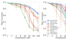
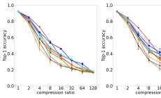
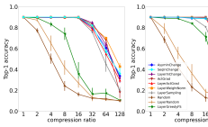
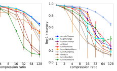
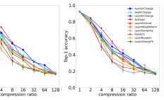
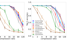
Figure 2: Top-1 Accuracy of different pruning methods, after fine-tuning with four batches of training data, applied to LeNet on MNIST (left), ResNet56 on CIFAR10 (middle), and VGG11 on CIFAR10 (right), for several compression ratios (in log-scale), with (top) and without (bottom) reweighting. We include the three reweighted variants of our method in the bottom plots (faded) for reference.

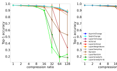
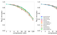
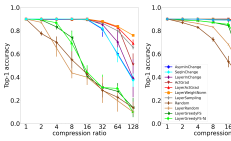
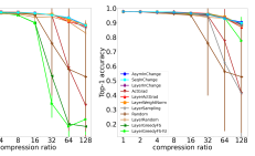
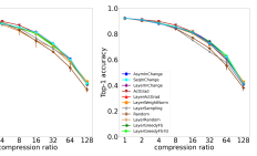
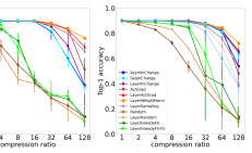
Figure 3: Top-1 Accuracy of different pruning methods, after fine-tuning with the full training data, applied to LeNet on MNIST (left), ResNet56 on CIFAR10 (middle), and VGG11 on CIFAR10 (right), for several compression ratios (in log-scale), with (top) and without (bottom) reweighting. We include the three reweighted variants of our method in the bottom plots (faded) for reference.

In this section, we study the effect of fine-tuning with both limited and sufficient data. To that end, we report the top-1 accuracy results of all the pruning tasks considered in Section 7, after fine-tuning with only four batches of training data, and after fine-tuning with the full training data in Figure 3. We fine-tune for 10 epochs in the MNIST experiment, and for 20 epochs in both CIFAR-10 experiments. We do not fine-tune at compression ratio 1 (i.e., when nothing is pruned).

Our method still outperforms other baselines after fine-tuning with limited-data, and is among the best performing methods even in the full-data setting (if we consider the non-reweighted variants for VGG11 model). As expected, fine-tuning with the full training data provides a significant boost in performance to all methods, even more than reweighting. Fine-tuning with limited data also helps but significantly less. Reweighting still improves the performance of all methods, except LAYERGREEDYFS and LAYERGREEDYFS-fd, even when fine-tuning with limited-data is used, but it can actually deteriorate performance when fine-tuning with full-data is used (see Figure 3 left-bottom plot, the reweighted variants of our methods have lower accuracy than the non-reweighted variants). We suspect that this could be due to overfitting to the very small training data used for pruning. This only happens with VGG11 model, because it is larger than LeNet and ResNet56 models. We expect the performance of the reweighted variants of our method to improve if we use more training data for pruning.

Appendix I Importance of per-layer budget selection

In this section, we study the effect of per-layer budget selection on accuracy. To that end, we use the same pretrained VGG11 model from Section 7, and prune the first and second to last convolution layers in it. Since the second to last layer in VGG11 (features.22) has little effect on accuracy when pruned, we expect the choice of how the global budget is distributed on the two layers to have a significant impact on performance. Figure 4 shows the top-1 accuracy for different fractions of prunable channels kept, when the per-layer budget selection from Section 5.2 is used, while Figure 5 shows the results when equal fractions of channels kept are used in each layer. As expected, all layerwise methods perform much more poorly with equal per-layer fractions, both with and without fine-tuning. Though, the difference is less drastic when fine-tuning is used.

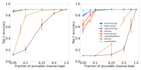
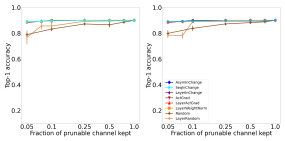
Figure 4: Top-1 Accuracy of different pruning methods on CIFAR10, after pruning the first and second to last convolution layers in VGG11 model, with different fractions of remaining channels (in log-scale), with (left) and without (right) reweighting, with (bottom) and without (top) fine-tuning, with per-layer fractions selected using the selection method discussed in Section 5.2. We include the three reweighted variants of our method in the plots without reweighting (faded) for reference.

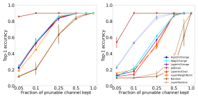
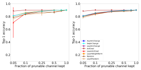
Figure 5: Top-1 Accuracy of different pruning methods on CIFAR10, after pruning the first and second to last convolution layers in VGG11 model, with different fractions of remaining channels (in log-scale), with (left) and without (right) reweighting, with (bottom) and without (top) fine-tuning, with equal per-layer fractions. We include the three reweighted variants of our method in the plots without reweighting (faded) for reference.

Appendix J Results with respect to other metrics

We report in Tables 3, 4 and 5, the top-1 accuracy, speedup ratio ($\tfrac{\text{original number of FLOPs}}{\text{pruned number of FLOPs}}$), and pruning time values of the experiments presented in Section 7. We exclude the worst performing methods Random and LayerRandom.

Note that for a given compression ratio speedup values vary significantly between different pruning methods, because the number of weights and flops vary between layers, and pruning methods differ in their per-layer budget allocations. The best performing methods in terms of compression are not necessarily the best ones in terms of speedup. For example, ActGrad is among the best performing methods in terms of compression on ResNet56-CIFAR10, but it is the worst one in terms of speedup. In cases where we care more about speedup than compression, we can replace the constraint in the per-layer budget selection problem (6) to be speedup instead of compression.

Since our goal in these experiments was to study performance in terms of accuracy vs compression rate, we did not focus on optimizing our method’s implementation for computation time efficiency. For example, our current implementation uses the classical Greedy algorithm. This can be significantly sped-up by switching to the faster Greedy algorithm from Li et al. [2022].

Table 3: Top-1 Accuracy % (Acc1), speedup ratio (SR), and pruning time (in hrs:mins:secs) of different pruning methods applied to LeNet on MNIST, with different compression ratios $c$, with and without reweighting (rw) and fine-tuning (ft).

$c=2$ $c=4$ $c=8$ $c=16$ $c=32$ Method rw ft Acc1 SR time Acc1 SR time Acc1 SR time Acc1 SR time Acc1 SR time ✓ ✓ 97.5 3.1 0:00:03 97.1 7.3 0:00:02 97.0 6.2 0:00:02 96.6 8.3 0:00:02 95.4 4.0 0:00:02 AsymInChange ✓ ✗ 97.4 3.1 0:00:03 96.2 7.3 0:00:02 94.4 6.2 0:00:02 90.3 8.3 0:00:02 83.5 4.0 0:00:02 ✗ ✓ 97.6 3.1 0:00:03 97.4 4.0 0:00:02 97.4 2.4 0:00:02 96.2 8.3 0:00:01 95.7 3.5 0:00:02 ✗ ✗ 84.6 3.1 0:00:03 48.7 4.0 0:00:02 36.4 2.4 0:00:02 12.8 8.3 0:00:01 14.4 3.5 0:00:02 ✓ ✓ 97.6 3.1 0:00:03 97.2 7.3 0:00:02 97.1 6.2 0:00:02 96.5 8.3 0:00:02 95.4 4.0 0:00:02 SeqInChange ✓ ✗ 97.4 3.1 0:00:03 95.8 7.3 0:00:02 94.3 6.2 0:00:02 89.7 8.3 0:00:02 82.2 4.0 0:00:02 ✗ ✓ 97.6 3.1 0:00:04 97.5 4.0 0:00:02 97.3 2.4 0:00:03 96.5 8.3 0:00:02 95.8 3.5 0:00:01 ✗ ✗ 88.5 3.1 0:00:04 39.0 4.0 0:00:02 25.8 2.4 0:00:03 12.4 8.3 0:00:02 10.7 3.5 0:00:01 ✓ ✓ 97.5 3.1 0:00:03 97.1 7.3 0:00:02 97.0 6.2 0:00:02 96.6 8.3 0:00:02 95.6 4.0 0:00:01 LayerInChange ✓ ✗ 97.4 3.1 0:00:03 95.8 7.3 0:00:02 94.2 6.2 0:00:02 89.9 8.3 0:00:02 81.8 4.0 0:00:01 ✗ ✓ 97.6 3.1 0:00:03 97.4 4.0 0:00:02 97.5 2.4 0:00:02 96.5 8.3 0:00:02 95.6 3.5 0:00:01 ✗ ✗ 88.6 3.1 0:00:03 40.6 4.0 0:00:02 33.5 2.4 0:00:02 23.9 8.3 0:00:02 13.1 3.5 0:00:01 ✓ ✓ 97.7 2.0 0:00:00 97.4 2.6 0:00:00 97.3 3.4 0:00:00 96.6 4.1 0:00:00 95.3 4.8 0:00:00 ActGrad ✓ ✗ 97.2 2.0 0:00:00 94.7 2.6 0:00:00 87.2 3.4 0:00:00 67.5 4.1 0:00:00 40.5 4.8 0:00:00 ✗ ✓ 97.6 2.0 0:00:00 97.5 2.6 0:00:00 97.2 3.4 0:00:00 96.6 4.1 0:00:00 95.0 4.8 0:00:00 ✗ ✗ 81.0 2.0 0:00:00 43.5 2.6 0:00:00 24.9 3.4 0:00:00 17.7 4.1 0:00:00 15.1 4.8 0:00:00 ✓ ✓ 97.6 3.1 0:00:00 97.1 4.7 0:00:00 96.6 11.2 0:00:00 95.8 16.2 0:00:00 95.8 4.0 0:00:00 LayerActGrad ✓ ✗ 97.1 3.1 0:00:00 95.1 4.7 0:00:00 90.2 11.2 0:00:00 82.9 16.2 0:00:00 76.9 4.0 0:00:00 ✗ ✓ 97.5 3.2 0:00:00 97.4 4.4 0:00:00 97.4 2.4 0:00:00 96.9 3.0 0:00:00 96.4 3.1 0:00:00 ✗ ✗ 84.9 3.2 0:00:00 46.3 4.4 0:00:00 27.9 2.4 0:00:00 20.5 3.0 0:00:00 17.0 3.1 0:00:00 ✓ ✓ 97.5 3.1 0:00:00 97.1 6.7 0:00:00 96.7 11.2 0:00:00 95.9 16.2 0:00:00 96.0 4.0 0:00:00 LayerWeightNorm ✓ ✗ 97.3 3.1 0:00:00 95.5 6.7 0:00:00 93.6 11.2 0:00:00 88.2 16.2 0:00:00 81.1 4.0 0:00:00 ✗ ✓ 97.5 3.0 0:00:00 97.5 3.0 0:00:00 97.3 2.6 0:00:00 96.0 14.7 0:00:00 95.8 3.5 0:00:00 ✗ ✗ 91.6 3.0 0:00:00 60.1 3.0 0:00:00 53.9 2.6 0:00:00 18.1 14.7 0:00:00 14.8 3.5 0:00:00 ✓ ✓ 97.5 1.9 0:00:20 97.4 2.7 0:00:21 97.0 3.5 0:00:19 96.4 4.4 0:00:20 95.7 5.2 0:00:19 LayerSampling ✓ ✗ 97.2 1.9 0:00:20 95.5 2.7 0:00:21 91.6 3.5 0:00:19 85.5 4.4 0:00:20 71.7 5.2 0:00:19 ✗ ✓ 97.6 1.9 0:00:19 97.3 2.7 0:00:20 96.8 3.5 0:00:18 96.1 4.4 0:00:19 94.4 5.2 0:00:18 ✗ ✗ 41.8 1.9 0:00:19 25.5 2.7 0:00:20 22.4 3.5 0:00:18 13.2 4.4 0:00:19 14.1 5.2 0:00:18 ✓ ✓ 97.3 3.3 0:00:33 96.9 4.9 0:00:27 95.2 7.4 0:00:40 90.0 10.4 0:00:19 53.3 9.0 0:00:28 LayerGreedyFS ✓ ✗ 94.1 3.3 0:00:33 88.1 4.9 0:00:27 76.2 7.4 0:00:40 44.9 10.4 0:00:19 23.8 9.0 0:00:28 ✗ ✓ 97.6 1.2 0:00:27 97.4 4.2 0:00:23 97.0 2.4 0:00:18 95.8 14.7 0:00:14 96.2 5.1 0:00:09 ✗ ✗ 73.5 1.2 0:00:27 45.0 4.2 0:00:23 28.0 2.4 0:00:18 28.3 14.7 0:00:14 20.1 5.1 0:00:09 ✓ ✓ 97.2 3.2 0:01:44 96.8 4.9 0:01:21 95.2 7.4 0:01:23 89.9 10.4 0:00:56 34.1 23.9 0:00:48 LayerGreedyFS-fd ✓ ✗ 94.2 3.2 0:01:44 88.2 4.9 0:01:21 75.8 7.4 0:01:23 47.2 10.4 0:00:56 17.2 23.9 0:00:48 ✗ ✓ 97.6 1.2 0:01:30 97.4 4.4 0:01:19 97.0 2.4 0:01:01 96.7 7.5 0:00:36 95.5 3.5 0:00:21 ✗ ✗ 73.5 1.2 0:01:30 47.4 4.4 0:01:19 30.3 2.4 0:01:01 23.3 7.5 0:00:36 16.9 3.5 0:00:21

Table 4: Top-1 Accuracy % (Acc1), speedup ratio (SR), and pruning time (in hrs:mins:secs) of different pruning methods applied to ResNet56 on CIFAR10,with different compression ratios $c$, with and without reweighting (rw) and fine-tuning (ft).

$c=2$ $c=4$ $c=8$ $c=16$ $c=32$ Method rw ft Acc1 SR time Acc1 SR time Acc1 SR time Acc1 SR time Acc1 SR time ✓ ✓ 90.7 2.6 2:13:10 87.9 6.0 1:14:00 84.9 11.0 0:42:08 81.1 16.4 0:24:43 72.1 21.3 0:14:57 AsymInChange ✓ ✗ 84.2 2.6 2:13:10 46.4 6.0 1:14:00 20.6 11.0 0:42:08 18.3 16.4 0:24:43 10.2 21.3 0:14:57 ✗ ✓ 90.9 2.5 2:15:09 88.3 6.0 1:12:51 85.4 10.4 0:40:31 81.7 15.1 0:26:00 74.2 20.2 0:15:23 ✗ ✗ 73.3 2.5 2:15:09 16.4 6.0 1:12:51 13.6 10.4 0:40:31 9.9 15.1 0:26:00 10.7 20.2 0:15:23 ✓ ✓ 90.7 2.6 4:13:21 88.0 6.0 2:50:54 85.2 11.0 1:30:23 81.1 16.4 0:48:09 72.6 21.3 0:24:36 SeqInChange ✓ ✗ 82.3 2.6 4:13:21 45.5 6.0 2:50:54 24.6 11.0 1:30:23 17.3 16.4 0:48:09 12.9 21.3 0:24:36 ✗ ✓ 90.9 2.5 4:01:33 88.3 6.0 2:41:17 85.5 10.4 1:29:22 81.4 15.1 0:46:34 72.7 20.2 0:22:47 ✗ ✗ 75.5 2.5 4:01:33 17.5 6.0 2:41:17 12.1 10.4 1:29:22 9.9 15.1 0:46:34 10.6 20.2 0:22:47 ✓ ✓ 90.7 2.6 4:20:16 88.0 6.0 2:53:00 85.1 11.0 1:38:14 81.5 16.4 0:51:46 72.6 21.3 0:24:11 LayerInChange ✓ ✗ 72.3 2.6 4:20:16 23.7 6.0 2:53:00 15.8 11.0 1:38:14 14.0 16.4 0:51:46 11.3 21.3 0:24:11 ✗ ✓ 90.9 2.5 4:21:26 88.4 6.0 2:49:09 85.4 10.4 1:29:47 81.9 15.1 0:49:17 73.4 20.2 0:22:33 ✗ ✗ 38.6 2.5 4:21:26 11.4 6.0 2:49:09 9.9 10.4 1:29:47 10.2 15.1 0:49:17 11.0 20.2 0:22:33 ✓ ✓ 91.3 1.7 0:02:07 89.8 2.6 0:02:22 86.8 4.2 0:01:47 81.0 6.7 0:01:55 71.3 10.8 0:01:31 ActGrad ✓ ✗ 85.2 1.7 0:02:07 50.4 2.6 0:02:22 21.3 4.2 0:01:47 14.1 6.7 0:01:55 11.4 10.8 0:01:31 ✗ ✓ 91.2 1.7 0:00:02 89.8 2.6 0:00:02 86.8 4.2 0:00:05 81.8 6.7 0:00:02 72.3 10.8 0:00:07 ✗ ✗ 50.3 1.7 0:00:02 16.4 2.6 0:00:02 10.5 4.2 0:00:05 11.7 6.7 0:00:02 10.2 10.8 0:00:07 ✓ ✓ 90.6 2.8 0:02:01 87.8 6.1 0:02:04 85.0 10.6 0:01:37 80.6 15.5 0:01:43 71.2 21.3 0:02:02 LayerActGrad ✓ ✗ 78.4 2.8 0:02:01 35.2 6.1 0:02:04 18.4 10.6 0:01:37 13.1 15.5 0:01:43 11.6 21.3 0:02:02 ✗ ✓ 90.5 2.9 0:00:06 88.4 5.7 0:00:05 85.3 10.1 0:00:10 81.6 15.1 0:00:10 72.2 20.2 0:00:05 ✗ ✗ 21.9 2.9 0:00:06 10.2 5.7 0:00:05 10.6 10.1 0:00:10 9.9 15.1 0:00:10 10.3 20.2 0:00:05 ✓ ✓ 90.8 2.7 0:02:14 88.4 5.8 0:01:48 84.9 10.3 0:01:47 80.8 16.4 0:01:30 71.7 21.3 0:01:39 LayerWeightNorm ✓ ✗ 81.8 2.7 0:02:14 46.7 5.8 0:01:48 20.4 10.3 0:01:47 12.0 16.4 0:01:30 11.0 21.3 0:01:39 ✗ ✓ 90.7 2.7 0:00:00 88.4 5.9 0:00:00 85.4 10.2 0:00:00 81.8 15.1 0:00:00 71.8 20.2 0:00:00 ✗ ✗ 25.4 2.7 0:00:00 9.9 5.9 0:00:00 9.4 10.2 0:00:00 9.9 15.1 0:00:00 9.8 20.2 0:00:00 ✓ ✓ 90.9 1.9 0:03:37 88.9 3.6 0:05:02 84.7 7.2 0:04:05 76.7 14.2 0:03:47 68.7 20.7 0:05:12 LayerSampling ✓ ✗ 79.2 1.9 0:03:37 32.7 3.6 0:05:02 14.0 7.2 0:04:05 11.8 14.2 0:03:47 10.3 20.7 0:05:12 ✗ ✓ 91.0 1.9 0:02:59 88.9 3.6 0:06:36 84.1 7.2 0:02:30 75.1 14.2 0:01:54 66.2 20.7 0:05:55 ✗ ✗ 26.0 1.9 0:02:59 11.9 3.6 0:06:36 11.0 7.2 0:02:30 9.5 14.2 0:01:54 9.5 20.7 0:05:55 ✓ ✓ 90.6 2.6 0:38:44 88.2 5.3 8:43:34 84.6 9.9 0:10:17 80.2 15.1 0:06:57 71.4 17.4 0:03:16 LayerGreedyFS ✓ ✗ 71.5 2.6 0:38:44 36.3 5.3 8:43:34 19.6 9.9 0:10:17 15.2 15.1 0:06:57 11.4 17.4 0:03:16 ✗ ✓ 90.8 2.6 0:30:11 88.6 5.7 0:36:54 85.5 9.7 0:19:09 80.7 16.4 0:04:44 73.0 21.3 0:02:05 ✗ ✗ 73.9 2.6 0:30:11 36.0 5.7 0:36:54 21.4 9.7 0:19:09 13.8 16.4 0:04:44 12.1 21.3 0:02:05 ✓ ✓ 90.6 2.6 6:54:48 88.4 5.6 0:21:51 85.0 9.9 4:19:50 80.0 15.2 0:07:27 70.6 17.4 0:06:58 LayerGreedyFS-fd ✓ ✗ 75.9 2.6 6:54:48 28.7 5.6 0:21:51 17.4 9.9 4:19:50 14.4 15.2 0:07:27 12.2 17.4 0:06:58 ✗ ✓ 90.7 2.6 1:09:55 88.6 5.7 0:25:45 85.6 9.3 0:18:38 81.1 15.3 0:11:40 74.3 22.0 0:04:07 ✗ ✗ 72.6 2.6 1:09:55 38.0 5.7 0:25:45 20.6 9.3 0:18:38 13.4 15.3 0:11:40 13.0 22.0 0:04:07

Table 5: Top-1 Accuracy % (Acc1), speedup ratio (SR), and pruning time (in hrs:mins:secs) of different pruning methods applied to VGG11 on CIFAR10, with different compression ratios $c$, with and without reweighting (rw) and fine-tuning (ft).

$c=2$ $c=4$ $c=8$ $c=16$ $c=32$ Method rw ft Acc1 SR time Acc1 SR time Acc1 SR time Acc1 SR time Acc1 SR time ✓ ✓ 89.7 1.9 31:38:06 89.7 2.1 30:35:13 89.6 2.5 23:54:22 89.5 5.0 22:38:37 81.4 8.3 19:01:51 AsymInChange ✓ ✗ 89.7 1.9 31:38:06 89.7 2.1 30:35:13 89.6 2.5 23:54:22 89.5 5.0 22:38:37 80.4 8.3 19:01:51 ✗ ✓ 90.1 1.9 34:15:16 90.1 2.1 33:33:05 89.3 2.5 24:58:50 89.1 4.7 18:59:56 87.6 6.8 16:52:36 ✗ ✗ 90.1 1.9 34:15:16 90.1 2.1 33:33:05 88.9 2.5 24:58:50 88.7 4.7 18:59:56 12.1 6.8 16:52:36 ✓ ✓ 90.1 1.9 30:29:41 90.1 2.1 30:31:14 90.0 2.5 23:25:17 89.8 5.0 25:04:38 81.9 8.3 23:54:55 SeqInChange ✓ ✗ 90.1 1.9 30:29:41 90.1 2.1 30:31:14 90.0 2.5 23:25:17 89.8 5.0 25:04:38 81.6 8.3 23:54:55 ✗ ✓ 90.1 1.9 32:17:12 90.1 2.1 31:13:02 89.3 2.5 23:51:44 89.3 4.7 22:31:17 87.7 6.8 20:23:53 ✗ ✗ 90.1 1.9 32:17:12 90.1 2.1 31:13:02 89.1 2.5 23:51:44 88.8 4.7 22:31:17 18.2 6.8 20:23:53 ✓ ✓ 90.1 1.9 27:27:33 90.1 2.1 29:43:24 90.0 2.5 20:45:59 89.8 5.0 29:00:23 85.3 8.3 18:56:08 LayerInChange ✓ ✗ 90.1 1.9 27:27:33 90.1 2.1 29:43:24 90.0 2.5 20:45:59 89.8 5.0 29:00:23 84.7 8.3 18:56:08 ✗ ✓ 90.1 1.9 36:41:49 90.1 2.1 34:49:36 89.2 2.5 29:05:17 89.1 4.7 21:39:32 87.8 6.8 20:45:04 ✗ ✗ 90.1 1.9 36:41:49 90.1 2.1 34:49:36 89.2 2.5 29:05:17 88.9 4.7 21:39:32 14.7 6.8 20:45:04 ✓ ✓ 90.1 3.2 0:00:58 90.1 3.4 0:01:17 90.1 3.6 0:01:28 90.1 4.9 0:00:59 88.0 10.2 0:00:54 ActGrad ✓ ✗ 90.1 3.2 0:00:58 90.1 3.4 0:01:17 90.1 3.6 0:01:28 90.1 4.9 0:00:59 83.2 10.2 0:00:54 ✗ ✓ 90.1 3.2 0:00:03 90.1 3.4 0:00:02 90.1 3.6 0:00:03 90.1 4.9 0:00:02 87.9 10.2 0:00:04 ✗ ✗ 90.1 3.2 0:00:03 90.1 3.4 0:00:02 90.1 3.6 0:00:03 90.1 4.9 0:00:02 56.8 10.2 0:00:04 ✓ ✓ 89.7 2.0 0:03:53 90.0 2.1 0:02:17 89.7 2.5 0:01:03 89.5 4.6 0:00:48 87.7 8.4 0:01:03 LayerActGrad ✓ ✗ 89.7 2.0 0:03:53 90.0 2.1 0:02:17 89.7 2.5 0:01:03 89.5 4.6 0:00:48 75.9 8.4 0:01:03 ✗ ✓ 90.1 1.9 0:00:05 90.1 2.0 0:00:06 90.1 2.6 0:00:05 89.5 5.0 0:00:06 87.2 5.5 0:00:08 ✗ ✗ 90.1 1.9 0:00:05 90.1 2.0 0:00:06 90.1 2.6 0:00:05 89.5 5.0 0:00:06 16.0 5.5 0:00:08 ✓ ✓ 90.1 1.8 0:01:52 90.1 2.0 0:00:53 90.0 2.5 0:00:46 89.8 5.0 0:01:08 88.1 8.3 0:00:52 LayerWeightNorm ✓ ✗ 90.1 1.8 0:01:52 90.1 2.0 0:00:53 90.0 2.5 0:00:46 89.8 5.0 0:01:08 80.9 8.3 0:00:52 ✗ ✓ 90.1 1.8 0:00:00 90.1 2.0 0:00:01 90.1 2.6 0:00:01 89.6 5.2 0:00:01 87.0 12.2 0:00:01 ✗ ✗ 90.1 1.8 0:00:00 90.1 2.0 0:00:01 90.1 2.6 0:00:01 89.6 5.2 0:00:01 11.6 12.2 0:00:01 ✓ ✓ 90.1 3.6 0:16:44 90.1 3.6 0:18:20 90.1 4.2 0:14:59 89.2 5.6 0:15:04 86.5 14.6 0:21:26 LayerSampling ✓ ✗ 90.1 3.6 0:16:44 90.1 3.6 0:18:20 90.1 4.2 0:14:59 89.2 5.6 0:15:04 75.0 14.6 0:21:26 ✗ ✓ 90.0 3.7 0:16:18 90.0 3.7 0:16:48 89.9 4.2 0:19:04 89.0 5.6 0:15:04 86.3 14.6 0:15:47 ✗ ✗ 90.0 3.7 0:16:18 90.0 3.7 0:16:48 89.9 4.2 0:19:04 50.5 5.6 0:15:04 13.7 14.6 0:15:47 ✓ ✓ 89.3 2.0 23:30:16 83.3 2.9 7:50:23 74.2 4.8 5:12:07 40.3 10.9 6:01:53 31.2 18.3 1:51:43 LayerGreedyFS ✓ ✗ 89.3 2.0 23:30:16 83.3 2.9 7:50:23 74.2 4.8 5:12:07 35.9 10.9 6:01:53 16.1 18.3 1:51:43 ✗ ✓ 89.2 2.0 9:49:18 88.7 2.2 6:56:45 87.2 2.8 4:10:47 84.4 4.8 2:40:57 46.4 7.4 2:36:44 ✗ ✗ 89.1 2.0 9:49:18 88.6 2.2 6:56:45 82.4 2.8 4:10:47 63.7 4.8 2:40:57 19.1 7.4 2:36:44 ✓ ✓ 89.4 2.0 12:06:03 86.8 2.7 10:22:33 69.1 4.0 6:00:33 44.3 13.0 3:27:58 31.1 13.0 3:35:15 LayerGreedyFS-fd ✓ ✗ 89.3 2.0 12:06:03 86.1 2.7 10:22:33 69.1 4.0 6:00:33 44.3 13.0 3:27:58 21.9 13.0 3:35:15 ✗ ✓ 89.4 2.0 12:42:58 88.6 2.6 7:40:45 87.1 3.3 5:04:15 85.5 4.9 3:45:22 63.5 11.5 1:59:09 ✗ ✗ 89.4 2.0 12:42:58 88.0 2.6 7:40:45 81.5 3.3 5:04:15 76.6 4.9 3:45:22 15.5 11.5 1:59:09

References

- Bian et al. [2017] A. A. Bian, J. M. Buhmann, A. Krause, and S. Tschiatschek. Guarantees for greedy maximization of non-submodular functions with applications. In Proceedings of the 34th International Conference on Machine Learning-Volume 70, pages 498–507. JMLR. org, 2017.
- Blalock et al. [2020] D. Blalock, J. J. G. Ortiz, J. Frankle, and J. Guttag. What is the state of neural network pruning? arXiv preprint arXiv:2003.03033, 2020.
- Bucila et al. [2006] C. Bucila, R. Caruana, and A. Niculescu-Mizil. Model compression. In Proceedings of the 12th ACM SIGKDD International Conference on Knowledge Discovery and Data Mining, KDD ’06, page 535–541, New York, NY, USA, 2006. Association for Computing Machinery. ISBN 1595933395. doi: 10.1145/1150402.1150464. URL https://doi.org/10.1145/1150402.1150464.
- Buschjäger et al. [2020] S. Buschjäger, P.-J. Honysz, and K. Morik. Very fast streaming submodular function maximization, 2020.
- Collins and Kohli [2014] M. D. Collins and P. Kohli. Memory bounded deep convolutional networks. arXiv preprint arXiv:1412.1442, 2014.
- Courbariaux et al. [2015] M. Courbariaux, Y. Bengio, and J.-P. David. Binaryconnect: Training deep neural networks with binary weights during propagations. In Advances in neural information processing systems, pages 3123–3131, 2015.
- Das and Kempe [2011] A. Das and D. Kempe. Submodular meets spectral: Greedy algorithms for subset selection, sparse approximation and dictionary selection. arXiv preprint arXiv:1102.3975, 2011.
- Denil et al. [2013] M. Denil, B. Shakibi, L. Dinh, M. A. Ranzato, and N. de Freitas. Predicting parameters in deep learning. In C. J. C. Burges, L. Bottou, M. Welling, Z. Ghahramani, and K. Q. Weinberger, editors, Advances in Neural Information Processing Systems, volume 26. Curran Associates, Inc., 2013. URL https://proceedings.neurips.cc/paper/2013/file/7fec306d1e665bc9c748b5d2b99a6e97-Paper.pdf.
- El Halabi et al. [2018] M. El Halabi, F. Bach, and V. Cevher. Combinatorial penalties: Structure preserved by convex relaxations. Proceedings of the 21st International Conference on Artificial Intelligence and Statistics, 2018.
- Elenberg et al. [2016] E. R. Elenberg, R. Khanna, A. G. Dimakis, and S. Negahban. Restricted strong convexity implies weak submodularity. arXiv preprint arXiv:1612.00804, 2016.
- Gong et al. [2014] Y. Gong, L. Liu, M. Yang, and L. Bourdev. Compressing deep convolutional networks using vector quantization. arXiv preprint arXiv:1412.6115, 2014.
- He et al. [2016] K. He, X. Zhang, S. Ren, and J. Sun. Deep residual learning for image recognition. In Proceedings of the IEEE conference on computer vision and pattern recognition, pages 770–778, 2016.
- He et al. [2014] T. He, Y. Fan, Y. Qian, T. Tan, and K. Yu. Reshaping deep neural network for fast decoding by node-pruning. In 2014 IEEE International Conference on Acoustics, Speech and Signal Processing (ICASSP), pages 245–249. IEEE, 2014.
- He et al. [2017] Y. He, X. Zhang, and J. Sun. Channel pruning for accelerating very deep neural networks. In Proceedings of the IEEE international conference on computer vision, pages 1389–1397, 2017.
- Hinton et al. [2015] G. Hinton, O. Vinyals, and J. Dean. Distilling the knowledge in a neural network. Neural Information Processing Systems (NeurIPS) Workshops, 2015.
- Hoefler et al. [2021] T. Hoefler, D. Alistarh, T. Ben-Nun, N. Dryden, and A. Peste. Sparsity in deep learning: Pruning and growth for efficient inference and training in neural networks. arXiv preprint arXiv:2102.00554, 2021.
- Krizhevsky et al. [2009] A. Krizhevsky, G. Hinton, et al. Learning multiple layers of features from tiny images. 2009.
- Kuzmin et al. [2019] A. Kuzmin, M. Nagel, S. Pitre, S. Pendyam, T. Blankevoort, and M. Welling. Taxonomy and evaluation of structured compression of convolutional neural networks. arXiv preprint arXiv:1912.09802, 2019.
- Lebedev et al. [2015] V. Lebedev, Y. Ganin, M. Rakhuba, I. V. Oseledets, and V. S. Lempitsky. Speeding-up convolutional neural networks using fine-tuned cp-decomposition. In International Conference on Learning Representations, 2015.
- LeCun et al. [1989] Y. LeCun, B. Boser, J. S. Denker, D. Henderson, R. E. Howard, W. Hubbard, and L. D. Jackel. Backpropagation applied to handwritten zip code recognition. Neural computation, 1(4):541–551, 1989.
- Lecun et al. [1998] Y. Lecun, C. Cortes, and C. Burges. The mnist databaseof handwritten digits, 1998.
- Lehmann et al. [2006] B. Lehmann, D. Lehmann, and N. Nisan. Combinatorial auctions with decreasing marginal utilities. Games and Economic Behavior, 55(2):270–296, 2006.
- Li et al. [2017] H. Li, A. Kadav, I. Durdanovic, H. Samet, and H. P. Graf. Pruning filters for efficient convnets. In 5th International Conference on Learning Representations, ICLR 2017, Toulon, France, April 24-26, 2017, Conference Track Proceedings. OpenReview.net, 2017. URL https://openreview.net/forum?id=rJqFGTslg.
- Li et al. [2022] W. Li, M. Feldman, E. Kazemi, and A. Karbasi. Submodular maximization in clean linear time, 2022. URL https://arxiv.org/abs/2006.09327.
- Liebenwein et al. [2020] L. Liebenwein, C. Baykal, H. Lang, D. Feldman, and D. Rus. Provable filter pruning for efficient neural networks. In International Conference on Learning Representations, 2020. URL https://openreview.net/forum?id=BJxkOlSYDH.
- Luo et al. [2017] J.-H. Luo, J. Wu, and W. Lin. Thinet: A filter level pruning method for deep neural network compression. In Proceedings of the IEEE international conference on computer vision, pages 5058–5066, 2017.
- Mariet and Sra [2015] Z. Mariet and S. Sra. Diversity networks: Neural network compression using determinantal point processes. arXiv preprint arXiv:1511.05077, 2015.
- McGuffie and Newhouse [2020] K. McGuffie and A. Newhouse. The radicalization risks of gpt-3 and advanced neural language models. arXiv preprint arXiv:2009.06807, 2020.
- Mirzasoleiman et al. [2015] B. Mirzasoleiman, A. Badanidiyuru, A. Karbasi, J. Vondrák, and A. Krause. Lazier than lazy greedy. In Proceedings of the AAAI Conference on Artificial Intelligence, volume 29, 2015.
- Molchanov et al. [2017] P. Molchanov, S. Tyree, T. Karras, T. Aila, and J. Kautz. Pruning convolutional neural networks for resource efficient inference. ICLR, 2017.
- Mussay et al. [2020] B. Mussay, M. Osadchy, V. Braverman, S. Zhou, and D. Feldman. Data-independent neural pruning via coresets. In International Conference on Learning Representations, 2020. URL https://openreview.net/forum?id=H1gmHaEKwB.
- Mussay et al. [2021] B. Mussay, D. Feldman, S. Zhou, V. Braverman, and M. Osadchy. Data-independent structured pruning of neural networks via coresets. IEEE Transactions on Neural Networks and Learning Systems, pages 1–13, 2021. doi: 10.1109/TNNLS.2021.3088587.
- Natarajan [1995] B. K. Natarajan. Sparse approximate solutions to linear systems. SIAM journal on computing, 24(2):227–234, 1995.
- Nemhauser et al. [1978] G. Nemhauser, L. Wolsey, and M. Fisher. An analysis of approximations for maximizing submodular set functions — I. Mathematical Programming, 14(1):265–294, 1978.
- Paszke et al. [2017] A. Paszke, S. Gross, S. Chintala, G. Chanan, E. Yang, Z. DeVito, Z. Lin, A. Desmaison, L. Antiga, and A. Lerer. Automatic differentiation in pytorch. 2017.
- Phan [2021] H. Phan. huyvnphan/pytorch_cifar10, Jan. 2021. URL https://doi.org/10.5281/zenodo.4431043.
- Simonyan and Zisserman [2015] K. Simonyan and A. Zisserman. Very deep convolutional networks for large-scale image recognition. In Y. Bengio and Y. LeCun, editors, 3rd International Conference on Learning Representations, ICLR 2015, San Diego, CA, USA, May 7-9, 2015, Conference Track Proceedings, 2015. URL http://arxiv.org/abs/1409.1556.
- Srinivas and Babu [2015] S. Srinivas and R. V. Babu. Data-free parameter pruning for deep neural networks. In Proceedings of the British Machine Vision Conference (BMVC), pages 31.1–31.12. BMVA Press, September 2015.
- Su et al. [2018] J. Su, J. Li, B. Bhattacharjee, and F. Huang. Tensorial neural networks: Generalization of neural networks and application to model compression. arXiv preprint arXiv:1805.10352, 2018.
- Sviridenko et al. [2017] M. Sviridenko, J. Vondrák, and J. Ward. Optimal approximation for submodular and supermodular optimization with bounded curvature. Mathematics of Operations Research, 42(4):1197–1218, 2017.
- Voita et al. [2019] E. Voita, D. Talbot, F. Moiseev, R. Sennrich, and I. Titov. Analyzing multi-head self-attention: Specialized heads do the heavy lifting, the rest can be pruned. In Proceedings of the 57th Annual Meeting of the Association for Computational Linguistics, pages 5797–5808, 2019.
- Ye et al. [2020a] M. Ye, C. Gong, L. Nie, D. Zhou, A. Klivans, and Q. Liu. Good subnetworks provably exist: Pruning via greedy forward selection. ICML, 2020a.
- Ye et al. [2020b] M. Ye, L. Wu, and Q. Liu. Greedy optimization provably wins the lottery: Logarithmic number of winning tickets is enough. Advances in Neural Information Processing Systems, 33:16409–16420, 2020b.
- Zhuang et al. [2018] Z. Zhuang, M. Tan, B. Zhuang, J. Liu, Y. Guo, Q. Wu, J. Huang, and J. Zhu. Discrimination-aware channel pruning for deep neural networks. In S. Bengio, H. Wallach, H. Larochelle, K. Grauman, N. Cesa-Bianchi, and R. Garnett, editors, Advances in Neural Information Processing Systems, volume 31. Curran Associates, Inc., 2018. URL https://proceedings.neurips.cc/paper/2018/file/55a7cf9c71f1c9c495413f934dd1a158-Paper.pdf.