Rethinking Task Sampling
for Few-shot Vision-Language Transfer Learning

Abstract

Despite achieving state-of-the-art zero-shot performance, existing vision-language models still fall short of few-shot transfer ability on domain-specific problems. Classical fine-tuning often fails to prevent highly expressive models from exploiting spurious correlations in the training data. Although model-agnostic meta-learning (MAML) presents as a natural alternative for few-shot transfer learning, the expensive computation due to implicit second-order optimization limits its use on large-scale vision-language models such as CLIP. While much literature has been devoted to exploring alternative optimization strategies, we identify another essential aspect towards effective few-shot transfer learning, task sampling, which is previously only be viewed as part of data pre-processing in MAML. To show the impact of task sampling, we propose a simple algorithm, Model-Agnostic Multitask Fine-tuning (MAMF), which differentiates classical fine-tuning only on uniformly sampling multiple tasks. Despite its simplicity, we show that MAMF consistently outperforms classical fine-tuning on five few-shot image classification tasks. We further show that the effectiveness of the bi-level optimization in MAML is highly sensitive to the zero-shot performance of a task in the context of few-shot vision-language classification. The goal of this paper is to provide new insights on what makes few-shot learning work, and encourage more research into investigating better task sampling strategies. Code and processed data are publicly available for research purposes at https://github.com/MikeWangWZHL/Multitask-Finetuning_CLIP

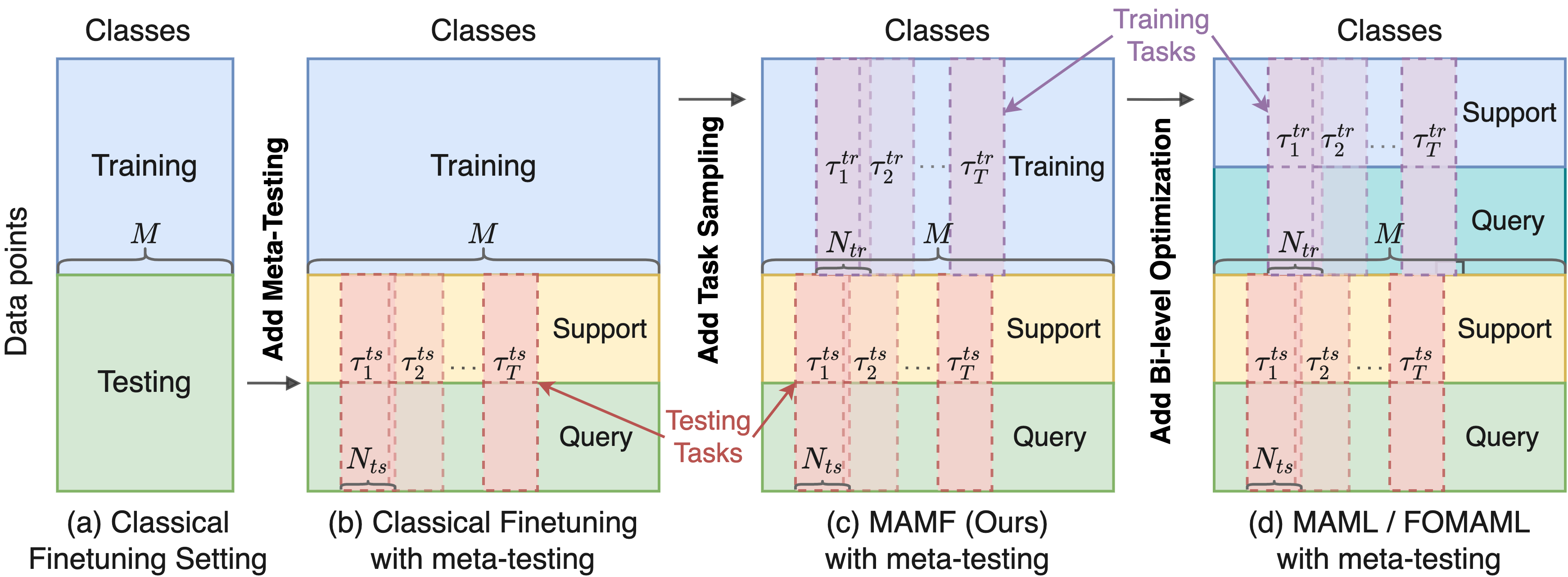
Figure 1: Task sampling and optimization schemes of different algorithms. Evaluation with meta-testing is applied in all of our experiments (b,c,d).

1 Introduction

While existing machine learning models have achieved human-level performance at various individual tasks, they generally lack the ability of fast adaptation and generalization. In recent years, transfer learning has been proven to be effective on a wide range of Computer Vision He et al. (2016); Dosovitskiy et al. (2020) and Natural Language Processing Devlin et al. (2019); Lewis et al. (2020) tasks. Specifically, recent advances in large-scale vision-language models Radford et al. (2021); Jia et al. (2021); Li et al. (2022); Alayrac et al. (2022) have demonstrated strong zero-shot ability on a wide range of tasks. However, these models still have certain limitations on concepts that require extensive domain knowledge, such as Fungi Classification. We identify two major limitations in current few-shot transfer learning literature, from both evaluation and algorithm perspective.

Limitation on evaluation   In current transfer learning paradigm, the testing instances of a downstream task are drawn from the same distribution as the training set. This evaluation setting can fail to faithfully reflect whether a model has truly learned a new concept, since modern deep neural networks can easily memorize and exploit spurious correlations from the training set Brown et al. (2020). Thus, we first propose a new evaluation scheme for few-shot transfer learning where we replace the original testing phase with meta-testing (Section 3). With meta-testing, the testing distribution are distinguished from the training.

Limitation on algorithm   To make an arbitrary pretrained vision-language model learn new concepts with few examples, model-agnostic meta-learning (MAML) Finn et al. (2017) presents as a natural candidate. One major limitation of the original MAML method is the expensive computation overhead due to implicit second-order optimization. Most follow-up work Finn et al. (2017); Nichol et al. (2018); Rajeswaran et al. (2019); Raghu et al. (2020); Von Oswald et al. (2021) has focused on improving the optimization strategy. However, we found that they all achieved comparable performance despite of using different optimization algorithms. This observation motivates us to ask: If the specific choice of optimization method is not the key to the empirical success of MAML, what would be?

Inspired by related work in the area of multitask learning Maurer et al. (2016); Tripuraneni et al. (2020), we conjecture that task sampling itself is an essential ingredient in learning new concepts efficiently. To verify this hypothesis, we propose a simple fine-tuning algorithm, Model-Agnostic Multitask Fine-tuning (MAMF), which simplifies MAML by using only first-order gradient-based optimization while keeping the uniform task sampling procedure intact. The goal is NOT to propose yet another complex algorithm, but to investigate what is the most important aspect for effective few-shot transfer learning. We compare MAMF with Classical Fine-tuning, which does not perform uniform task sampling, and first-order MAML (FOMAML) Finn et al. (2017), which adopts complex bi-level optimization upon sampled tasks. Our empirical result demonstrates the importance of uniform task sampling and reveals limited effectiveness of the bi-level optimization of MAML in the context of few-shot transfer learning. We hope our work encourages more research into exploring better task sampling strategies for improving few-shot transfer learning and meta-learning algorithms.

2 Problem Formulation

We are interested in a few-shot classification problem where we have a pretrained vision-language model $f$ with initial parameters $\bm{\theta}$. Let $\tau^{tr}$ be a training task sampled from a distribution $p(\tau^{tr})$, and $\tau^{ts}$ be a testing task sampled from $p(\tau^{ts})$, where a task is defined to an induced sub-problem by restricting the output space from the original problem. Specifically, for an original classification problem with $M$ classes in total, we define a task as a sub-problem where the output space is a subset of $N$ classes randomly sampled from the $M$ classes. We further denote $N^{tr}$ and $N^{ts}$ as the number of classes in each training and testing task. $T^{tr}$ and $T^{ts}$ as the total number of sampled tasks respectively. The Classical Fine-tuning setting is depicted in Figure 1 (a), where we have $T^{tr}=1$ training tasks with $N^{tr}=M$ classes, and $T^{ts}=1$ testing tasks with $N^{ts}=M$ classes. That is, both training and testing sets are treated as one single task containing data points from all $M$ classes.

3 Reformulating Classical Fine-tuning Evaluation with Meta-testing

Our goal is to enable and evaluate a model’s capability of generalizing to new concepts with few examples. The Classical Fine-tuning setting is not sufficient since the training and testing data points are drawn from the same distribution. Therefore, we propose to replace the original joint testing in Classical Fine-tuning with meta-testing.

Meta-testing is first introduced by related work in meta-learning  Thrun and Pratt (2012); Vinyals et al. (2016); Finn et al. (2017). As shown in the testing phase of Figure 1 (b,c,d), we first sample $T^{ts}$ tasks ($T^{ts}>1$), each containing data points from $N^{ts}$ classes ($1<N^{ts}<M$). For each sampled testing task $\tau^{ts}$, we further randomly split the data points into two disjoint sets, i.e., support set $A$ and query set $B$, with corresponding loss $\mathcal{L}_{\tau^{ts},A}$ and $\mathcal{L}_{\tau^{ts},B}$. Then we further update the model parameters on the support set and evaluate on the query set. By randomly sampling multiple tasks during meta-testing, we can distinguish the testing distribution from training, which largely prevents the model from exploiting spurious correlations in the training set. Essentially, we make the original problem more challenging by requiring the model to quickly generalize to potentially unseen task distributions during testing. The objective is to find an updated model parameter $\widetilde{\bm{\theta}}$ that minimizes the expected loss on all testing tasks $\mathbb{E}_{\tau^{ts}\sim p(\tau^{ts})}\left[\mathcal{L}_{\tau^{ts}}(\widetilde{\bm{\theta}})\right]$. Specifically, under this setting, MAML’s objective can be written as follows:

$$\min_{\widetilde{\bm{\theta}}}\mathbb{E}_{\tau^{ts}\sim p(\tau^{ts})}\left[\mathcal{L}_{\tau^{ts},B}\left(U_{\tau^{ts},A}^{ts}(\widetilde{\bm{\theta}})\right)\right],$$

$$\;\;\widetilde{\bm{\theta}}=\min_{\bm{\theta}}\mathbb{E}_{\tau^{tr}\sim p(\tau^{tr})}\left[\mathcal{L}_{\tau^{tr},B}\left(U_{\tau^{tr},A}^{tr}(\bm{\theta})\right)\right]$$

where $U_{\tau^{tr},A}^{tr}$ is the optimization procedure that updates the initial parameter $\bm{\theta}$ for one or more steps on the support set of a training task $\tau^{tr}$.

4 Model-Agnostic Multitask Fine-tuning

As shown above, previous MAML-like methods update model parameters iteratively via a complex bi-level optimization scheme Finn et al. (2017); Raghu et al. (2020); Rajeswaran et al. (2019), which is computationally expensive. We hypothesize that the task sampling process itself is more important than specific choice of optimization method. To verify this hypothesis, we propose a simple algorithm, Model-Agnostic Multitask Fine-tuning (MAMF), where we keep the uniform task sampling strategy as MAML but perform simple first-order gradient-based optimization on each task sequentially. Unlike MAML, MAMF does not further split the tasks into support and query sets. The objective of MAMF can be written as:

$$\min_{\widetilde{\bm{\theta}}}\mathbb{E}_{\tau^{ts}\sim p(\tau^{ts})}\left[\mathcal{L}_{\tau^{ts},B}\left(U_{\tau^{ts},A}^{ts}(\widetilde{\bm{\theta}})\right)\right]$$

$$\widetilde{\bm{\theta}}=\bm{\theta}_{i=T^{tr}},\bm{\theta}_{i}=U^{tr}_{\tau^{tr}_{i}}(\bm{\theta}_{i-1}),i\in\{1,2,...,T^{tr}\}$$

where $\bm{\theta}_{0}=\bm{\theta}$ and $U^{tr}_{\tau^{tr}_{i}}$ is the optimization procedure that updates the parameters from the previous task on the current training task $\tau^{tr}_{i}$. MAMF can also be viewed as a simplified version of Reptile Nichol et al. (2018), where we further eliminate the hyper-parameter of step size. The goal is to keep the algorithm as simple as possible to distinguish the impact of task sampling. Figure 1 depicts a comparison of different data sampling and optimization schemes of different algorithms.

5 Experiment

5.1 Experimental Setup

We aim to investigate two main questions experimentally under a few-shot vision-language transfer learning setting:

• Q1: Is the uniform task sampling during training important?

• Q2: Is the bi-level optimization in MAML consistently effective?

To answer the first question, we compare MAMF with Classical Fine-tuning where the only difference is the additional uniform task sampling. For the second question, we compare FOMAML and MAMF.

We perform comprehensive experiments on five few-shot image-classification datasets with various domains, including ClevrCounting Johnson et al. (2017), Amazon Berkeley Objects (ABO) Collins et al. (2021) Material, Fungi Su et al. (2021), Mini-Imagenet Vinyals et al. (2016), Caltech-UCSD Birds 200 (CUB) Welinder et al. (2010). We compare different learning algorithms by applying them to a large-scale vision-language model, i.e., CLIP Radford et al. (2021). We adopt the contrastive classification framework following Radford et al. (2021) where we directly match prompted label text with encoded images. This framework allows us to avoid the label permutation problem raised by Ye and Chao (2021). Details on the datasets and the classification framework can be found in Appendix A and  B.

Given a dataset with $M$ classes in total, we experiment with various task configurations regarding the number of sub-sampled classes $N^{ts}$, where $2\leq N^{ts}\leq M$. That is, during meta-testing, each task can be formulated as a $N^{ts}$-way classification and we randomly sample $T^{ts}$ such tasks. During training, for Classical Fine-tuning, we set the training task configuration as $N^{tr}=M,T^{tr}=1$; for MAMF and FOMAML, we set $N^{tr}=N^{ts}=N,T^{tr}=T^{ts}=T$, where $T$ is determined based on $N$ to cover all classes with a high probability. Implementation details can be found in Appendix C.

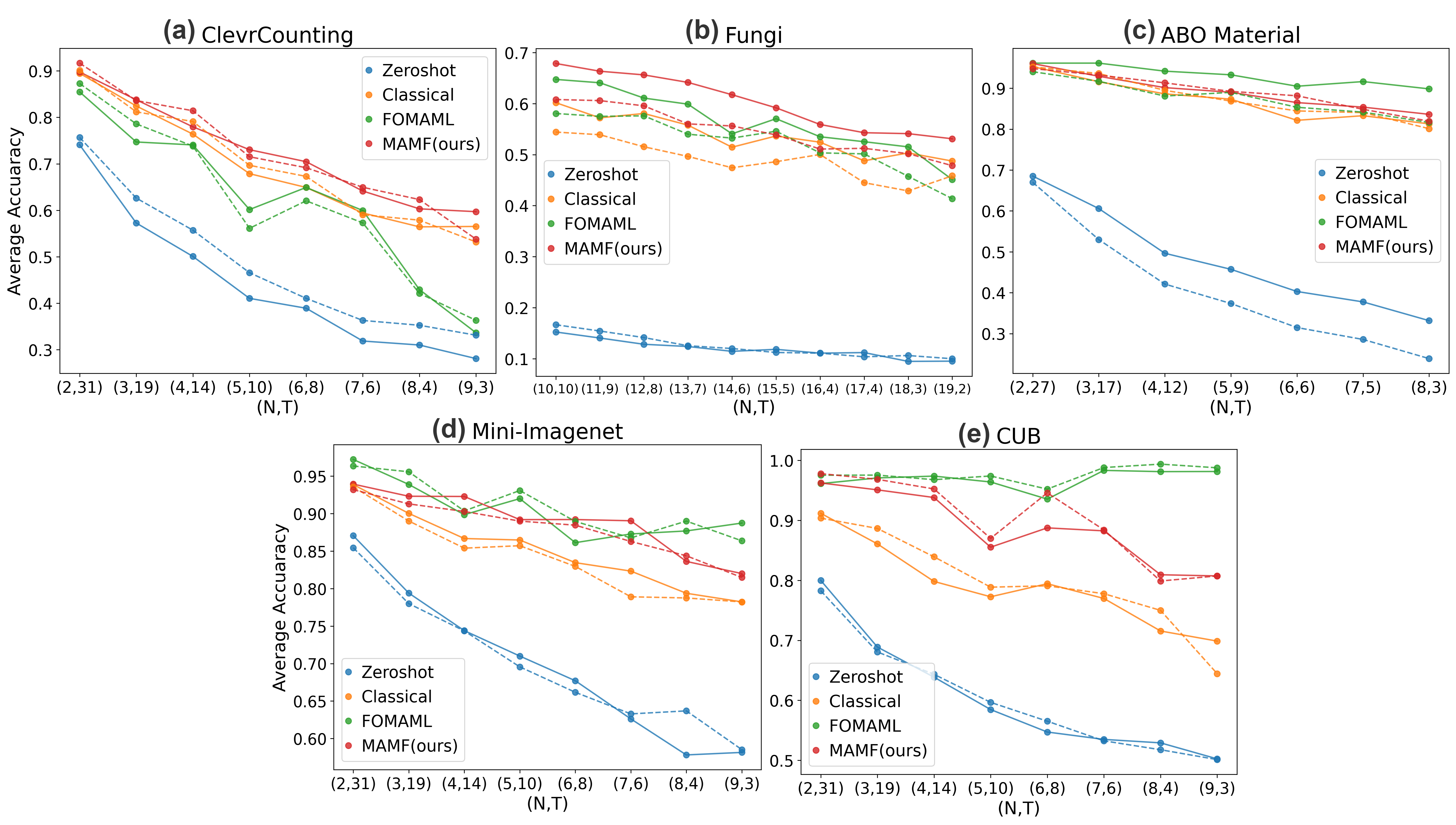
Figure 2: Average accuracy on development sets (dashed line) and test sets (solid line) of five datasets. The x-axis shows the task configurations where $(N,T)$ refers to sampling $T$ tasks for $N$-way classification. Zeroshot refers to zero-shot CLIP without any fine-tuning during either training or meta-testing. Classical refers to classical fine-tuning where we perform joint training on the entire training set. Both FOMAML and MAMF sample $N$-way $T$ tasks during training. MAMF consistently outperforms Classical on all datasets.

5.2 Results

Answer to Q1: Uniform task sampling is important. As depicted in Figure 2, comparing the performance of MAMF (red line) and Classical Fine-tuning (yellow line), MAMF consistently outperforms Classical Fine-tuning on all five datasets. Recall that the only difference between MAMF and Classical Fine-tuning is whether they perform uniform task sampling during training. This empirical result shows that task sampling itself serves as an important procedure for learning new concepts in a few-shot setting, even if with its simplest form, i.e. uniform sampling.

Answer to Q2: MAML is not effective on learning initially challenging problems. One unexpected observation from Figure 2 is that, although FOMAML has the same task sampling procedure and more sophisticated optimization method than MAMF, it is outperformed by MAMF on many tasks. We find that the effectiveness of FOMAML is highly sensitive to the zero-shot performance of the target task. Whenever the task is initially more challenging, i.e., with lower zero-shot performance, FOMAML tends to be less effective. For example, on CUB (Figure 2 e) where the zero-shot accuracy ranges from $0.5$ to $0.8$, FOMAML outperforms other algorithms in most cases. However, on ClevrCounting (Figure 2 a) where the zero-shot accuracy ranges from $0.3$ to $0.75$, MAMF and even Classical Fine-tuning consistently outperform FOMAML. To further visualize this correlation, we plot a Winner Map (Figure 3) which depicts the best-performing method for each task configuration on all datasets. We can see a clear pattern showing that FOMAML is only effective when the zero-shot performance is already high, while MAMF dominates on initially more challenging tasks.

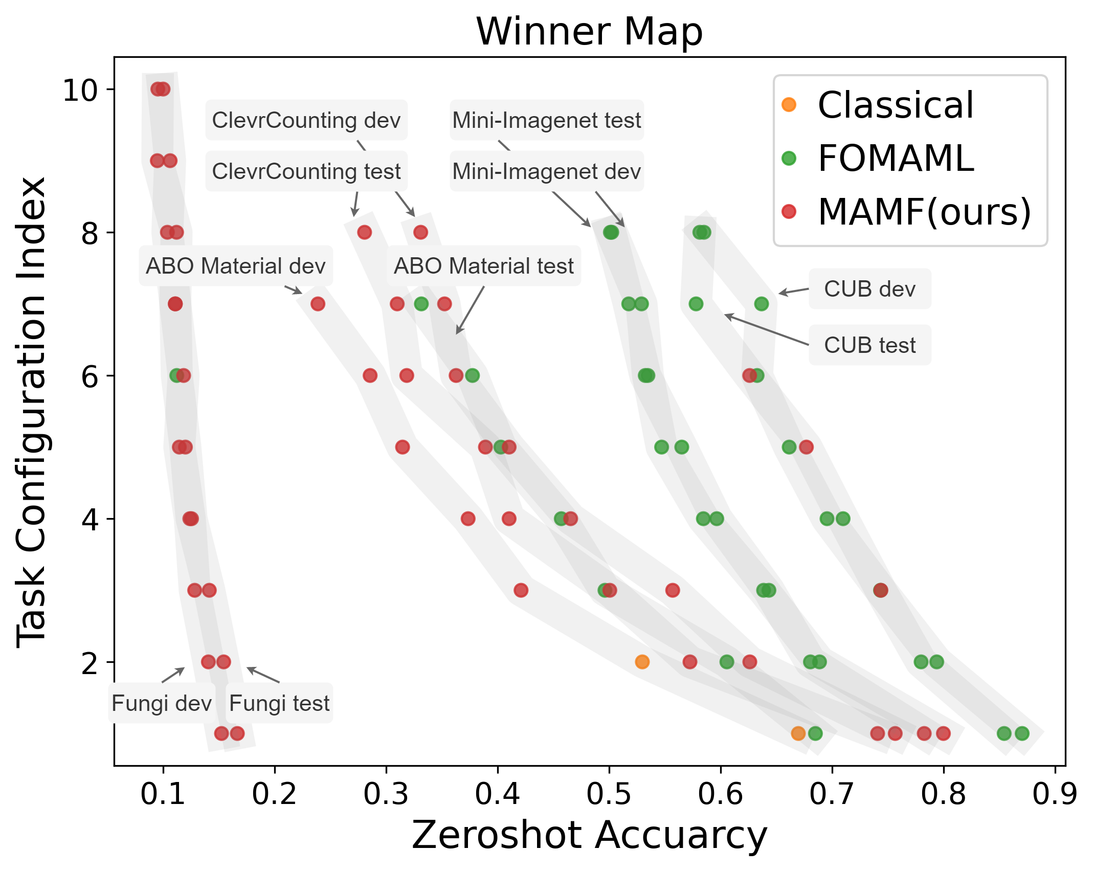
Figure 3: Each thick shaded line represents a dataset split, e.g., test set of ClevrCounting. Each dot corresponds to one task configuration in Figure 2 such as $(N=5,T=10)$. The color of a dot represents the best-performing algorithm. MAMF tends to outperform other algorithms when the problem is initially more challenging, i.e., when zero-shot accuracy is lower.

6 Conclusion

In this paper, We demonstrate the importance of task sampling by proposing a simple yet effective fine-tuning method MAMF. We further show novel insights on the limited effectiveness of the bi-level optimization. We hope our work encourages more research on improving few-shot transfer learning via better task sampling beyond uniform sampling.

Appendix A Dataset Details

In this work, we compare few-shot image classification performance on five datasets representing various concepts including: ClevrCounting Johnson et al. (2017), Amazon Berkeley Objects (ABO) Collins et al. (2021) Material, Fungi Su et al. (2021), Mini-Imagenet Vinyals et al. (2016), Caltech-UCSD Birds 200 (CUB) Welinder et al. (2010). We randomly split each dataset into disjoint training, development, and test sets, and perform subsampling to frame the experiments in a few-shot setting. Specifically, for ABO Material, we construct a subset of the original dataset by clustering images according to their Material attribute. We then manually filter out noisy samples that have multiple major materials. Table 1 shows the statistics of each dataset.

We selectively add data augmentation for different datasets. By default we use RandomResizedCrop, RandomHorizontalFlip and Normalize for all our five datasets. We further add ColorJitter for Mini-Imagenet and ClevrCounting. We disable ColorJitter for CUB, Fungi, and ABO Material since the color feature is essential for doing classification on these datasets. Following the original CLIP paper Radford et al. (2021), the input images are resized to 224$\times$224.

Dataset	$M$	$S^{tr}$	$S^{ts}_{A}$	$S^{ts}_{B}$
ClevrCounting	10	60	10	10
Fungi	20	60	10	10
ABO Material	9	50	15	15
Mini Imagenet	10	60	10	10
CUB	10	60	10	10

Table 1: Dataset statistics. $M$ is the total number of classes; $S^{tr}$ is the number of training samples per class; $S^{ts}_{A}$ and $S^{ts}_{B}$ are the number of support set and query set samples per class during meta-testing respectively.

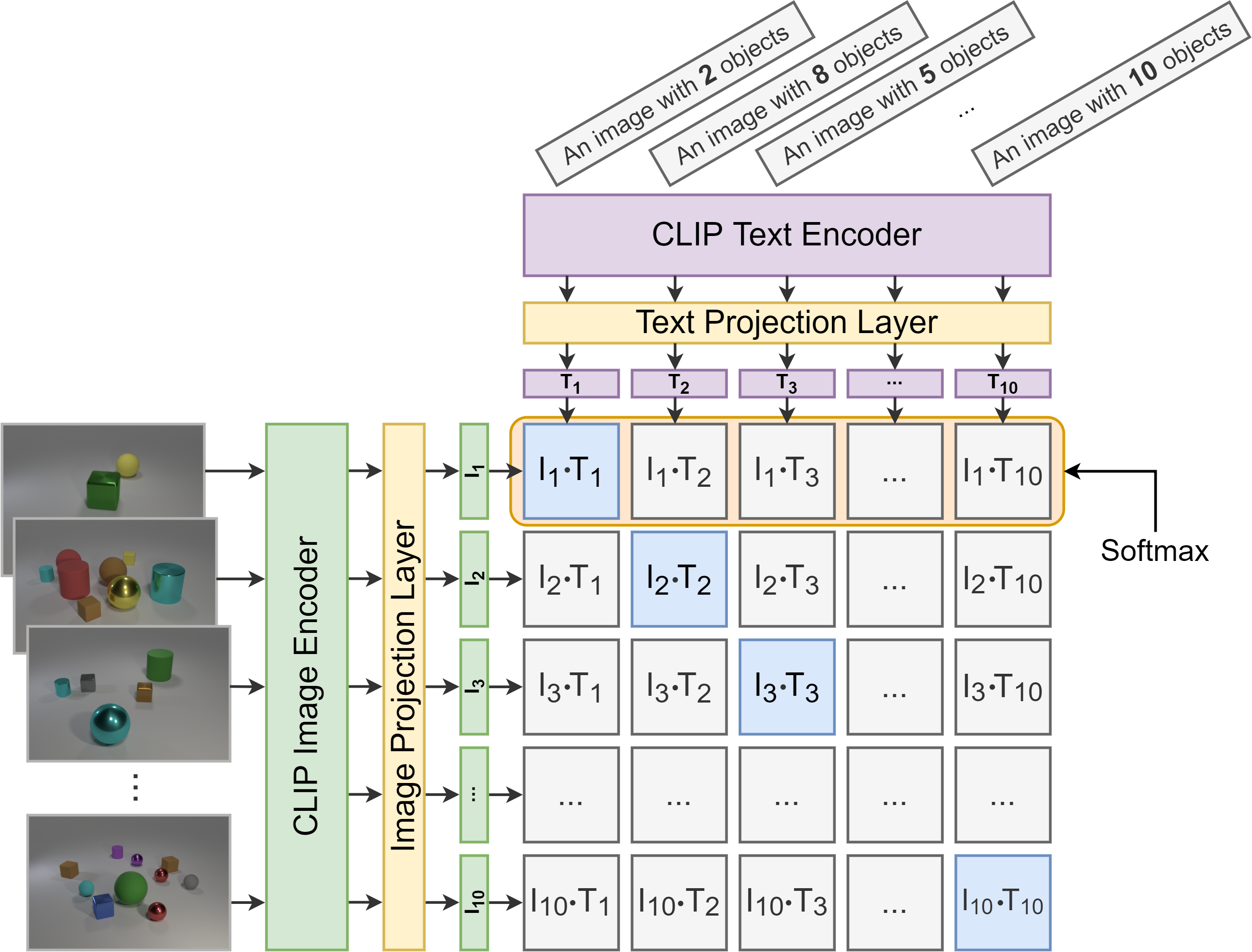
Figure 4: An illustration of the contrastive classification framework. We show a 10-way classification task on the Clevrcounting dataset. Each entry in the matrix is the similarity score (dot product) of an image embedding I and a text embedding T.

Appendix B Contrastive Image Classification Framework

We compare three algorithms (Classical Fine-tuning, MAML Fine-tuning, and MAMF) using an a contrastive classification framework based on pretrained CLIP Radford et al. (2021). Instead of using a linear output layer mapping to $N$ logits corresponding to $N$ class labels, we directly compute the similarity between candidate text embeddings representing each class with the image embedding. Specifically, we create the text representation for each class by using template prompts filled with label names. A full list of templates we use for each dataset can be found in Table 2. Figure 4 shows an example task from the ClevrCounting dataset, where each class is represented as a string such as “An image with 2 objects". We then compute the dot product of each $<$image, text$>$ embedding pairs. For each row, the label with the highest similarity score is selected as the final prediction.

Dataset	Text Input Template Example
ClevrCounting	An image of $<$8$>$ objects.
Fungi	A photo of $<$mycena pura$>$.
ABO Material	An image of a product made of $<$glass$>$
Mini Imagenet	A photo of $<$walker hound$>$.
CUB	A photo of $<$baltimore oriole$>$.

Table 2: Example templates with filled labels for all five datasets.

Appendix C Implementation Details

We use the pretrained CLIPRadford et al. (2021) with a ViT-B/32 Vision Transformer as image encoder and a masked self-attention Transformer as text encoder. The image embedding size is $768$ and the text embedding size is $512$. During training, we take the pre-projection image/text representation from the pretrained image/text encoder and feed them into a newly initialized image/text projection layer. We choose the pre-projection representation as prior work Chen et al. (2020) has shown that in such contrastive models the hidden layer before the last projection head serves as a better representation. Finally, we obtain an image embedding and a text embedding with the same size of 512. Note that for the Zeroshot baseline, we use the original projection layer and directly test on the query set in meta-testing without any fine-tuning. We train the model using cross-entropy loss for all three algorithms. We use the Adam optimizer Kingma and Ba (2015) with learning rate $1e-6$ during training and $1e-7$ during meta-testing. No weight decay is used for all algorithms during training and meta-testing. We use the MAML wrapper from learn2learnArnold et al. (2020) for training using first-order MAML.

Appendix D Detailed Results

Table 3 shows the detailed accuracy and standard deviation on the development sets and test sets of all the datasets shown in Figure 2 in the main paper. The $(N,T)$ column represents the task configurations, where $N$ stands for an $N$-way classification task and $T$ stands for the total number of sampled tasks. Since the tasks are randomly sampled from the class distribution, in order to cover all classes with high probability during testing, we set the number of sampled tasks to be: $T=\frac{log(0.001)}{log(1-\frac{N}{M})}$, where $M$ is the total number of classes. That is, with probability higher than $0.999$, we can cover all classes if sampling $T$ tasks. Columns with name Zeroshot, Classical, MAMF, and FOMAML represent models using Zeroshot CLIP, Classical Fine-tuning, Model-Agnostic Multitask Fine-tuning and first-order MAML respectively. The superscript on each accuracy percentage number indicates standard deviation across five random runs.

Table 3: Detailed average accuracy (%) and standard deviation on the development set and test set of all five datasets. The (N, T) column represents the task configurations consistent with the x-axis in Figure 3 in the main paper. Note that for the ABO Material dataset, we have 9 classes in total, so a task has up to 8-way classification. And for the Fungi dataset, which has 20 classes in total, we test on 10-way to 19-way classification tasks.

Dataset	(N, T)	Zeroshot	Classical	MAMF	FOMAML	Dataset	(N, T)	Zeroshot	Classical	MAMF	FOMAML
	(2, 27)	${68.5}^{2.6}$	${95.3}^{1.8}$	${96.0}^{1.8}$	${\textbf{96.1}}^{2.4}$		(2, 27)	${67.0}^{2.6}$	${95.2}^{0.6}$	${\textbf{94.8}}^{1.2}$	${94.0}^{0.4}$
	(3, 17)	${60.6}^{6.0}$	${91.6}^{3.0}$	${92.9}^{2.4}$	${\textbf{96.1}}^{1.0}$		(3, 17)	${53.0}^{1.9}$	${\textbf{93.6}}^{0.9}$	${93.2}^{0.9}$	${91.7}^{1.3}$
ABO	(4, 12)	${49.6}^{3.4}$	${88.6}^{0.6}$	${90.1}^{0.7}$	${\textbf{94.2}}^{1.6}$	ABO	(4, 12)	${42.1}^{2.8}$	${89.5}^{2.5}$	${\textbf{91.3}}^{2.2}$	${88.1}^{1.7}$
Material	(5, 9)	${45.7}^{1.6}$	${87.3}^{1.5}$	${89.0}^{1.2}$	${\textbf{93.3}}^{0.7}$	Material	(5, 9)	${37.4}^{2.6}$	${86.8}^{2.2}$	${\textbf{89.2}}^{1.4}$	${89.0}^{1.4}$
Test	(6, 6)	${40.3}^{2.1}$	${82.1}^{2.1}$	${86.5}^{2.5}$	${\textbf{90.5}}^{1.4}$	Dev	(6, 6)	${31.5}^{1.8}$	${84.4}^{1.6}$	${\textbf{88.1}}^{3.2}$	${85.3}^{2.9}$
	(7, 5)	${37.8}^{3.4}$	${83.3}^{3.0}$	${85.4}^{4.0}$	${\textbf{91.6}}^{1.7}$		(7, 5)	${28.6}^{2.0}$	${84.0}^{1.5}$	${\textbf{84.8}}^{1.2}$	${84.2}^{3.1}$
	(8, 3)	${33.2}^{0.7}$	${81.3}^{0.8}$	${83.6}^{1.6}$	${\textbf{89.8}}^{0.9}$		(8, 3)	${23.9}^{2.7}$	${80.1}^{1.3}$	${\textbf{81.9}}^{1.8}$	${81.6}^{1.2}$
	(2, 31)	${74.1}^{2.2}$	${89.5}^{1.7}$	${\textbf{89.8}}^{1.5}$	${85.5}^{2.2}$		(2, 31)	${75.7}^{3.4}$	${90.1}^{2.7}$	${\textbf{91.7}}^{2.5}$	${87.3}^{1.4}$
	(3, 19)	${57.3}^{2.1}$	${82.5}^{3.3}$	${\textbf{83.8}}^{3.8}$	${74.7}^{4.5}$		(3, 19)	${62.6}^{1.5}$	${81.2}^{2.5}$	${\textbf{83.6}}^{3.0}$	${78.6}^{4.5}$
Clevr-	(4, 14)	${50.1}^{2.0}$	${76.4}^{2.0}$	${\textbf{78.0}}^{3.3}$	${74.1}^{1.6}$	Clevr-	(4, 14)	${55.7}^{1.9}$	${79.1}^{2.0}$	${\textbf{81.4}}^{1.1}$	${73.8}^{5.3}$
Counting	(5, 10)	${41.0}^{2.5}$	${67.9}^{3.0}$	${\textbf{73.0}}^{2.8}$	${60.2}^{9.5}$	Counting	(5, 10)	${46.6}^{3.7}$	${69.7}^{4.6}$	${\textbf{71.5}}^{6.1}$	${56.1}^{0.9}$
Test	(6, 8)	${38.9}^{2.6}$	${64.9}^{3.9}$	${\textbf{70.5}}^{3.0}$	${64.9}^{5.0}$	Dev	(6, 8)	${41.0}^{1.3}$	${67.3}^{2.6}$	${\textbf{69.2}}^{5.2}$	${62.0}^{3.6}$
	(7, 6)	${31.9}^{0.9}$	${59.4}^{3.3}$	${\textbf{64.1}}^{1.7}$	${60.0}^{6.9}$		(7, 6)	${36.3}^{1.9}$	${59.0}^{4.8}$	${\textbf{65.0}}^{4.2}$	${57.3}^{1.9}$
	(8, 4)	${31.0}^{1.3}$	${56.4}^{5.8}$	${\textbf{60.3}}^{3.2}$	${42.9}^{5.6}$		(8, 4)	${35.3}^{1.2}$	${57.9}^{4.6}$	${\textbf{62.3}}^{3.5}$	${42.1}^{9.2}$
	(9, 3)	${28.1}^{1.2}$	${56.5}^{3.1}$	${\textbf{59.7}}^{4.8}$	${33.6}^{13.2}$		(9, 3)	${33.1}^{2.3}$	${53.2}^{3.3}$	${\textbf{53.8}}^{2.6}$	${36.3}^{12.6}$
	(2, 31)	${80.0}^{2.6}$	${91.2}^{1.6}$	${\textbf{96.2}}^{1.8}$	${96.1}^{2.9}$		(2, 31)	${78.3}^{1.1}$	${90.4}^{1.9}$	${\textbf{97.8}}^{1.5}$	${97.5}^{1.4}$
	(3, 19)	${68.9}^{1.6}$	${86.1}^{5.6}$	${95.1}^{0.9}$	${\textbf{97.1}}^{3.3}$		(3, 19)	${68.1}^{2.3}$	${88.7}^{7.1}$	${96.8}^{2.3}$	${\textbf{97.5}}^{2.5}$
	(4, 14)	${63.9}^{3.3}$	${79.8}^{4.4}$	${93.8}^{2.6}$	${\textbf{97.4}}^{1.9}$		(4, 14)	${64.3}^{1.9}$	${83.9}^{4.6}$	${95.2}^{2.8}$	${\textbf{96.8}}^{2.8}$
CUB	(5, 10)	${58.5}^{2.6}$	${77.3}^{3.3}$	${85.5}^{6.6}$	${\textbf{96.4}}^{1.4}$	CUB	(5, 10)	${59.7}^{2.3}$	${78.9}^{5.4}$	${87.0}^{6.2}$	${\textbf{97.4}}^{2.2}$
Test	(6, 8)	${54.7}^{2.0}$	${79.4}^{5.5}$	${88.8}^{3.0}$	${\textbf{93.5}}^{5.6}$	Dev	(6, 8)	${56.5}^{1.3}$	${79.1}^{0.6}$	${94.6}^{3.1}$	${\textbf{95.2}}^{5.2}$
	(7, 6)	${53.5}^{1.9}$	${77.0}^{7.9}$	${88.3}^{3.5}$	${\textbf{98.3}}^{0.3}$		(7, 6)	${53.3}^{2.0}$	${77.8}^{3.4}$	${88.4}^{3.9}$	${98.8}^{0.0}$
	(8, 4)	${52.9}^{2.6}$	${71.6}^{7.4}$	${80.9}^{3.8}$	${\textbf{98.1}}^{0.5}$		(8, 4)	${51.8}^{1.7}$	${75.0}^{7.2}$	${79.9}^{4.7}$	${99.4}^{0.4}$
	(9, 3)	${50.2}^{1.3}$	${69.9}^{5.1}$	${80.7}^{4.1}$	${\textbf{98.1}}^{0.7}$		(9, 3)	${50.1}^{2.5}$	${64.4}^{8.3}$	${80.7}^{3.3}$	${\textbf{98.8}}^{0.9}$
	(2, 31)	${87.1}^{1.4}$	${93.9}^{1.5}$	${93.9}^{1.5}$	${\textbf{97.2}}^{1.4}$		(2, 31)	${85.5}^{2.7}$	${93.6}^{0.7}$	${93.2}^{3.0}$	${\textbf{96.4}}^{0.4}$
	(3, 19)	${79.4}^{2.3}$	${90.0}^{1.6}$	${92.3}^{1.5}$	${\textbf{93.9}}^{2.6}$		(3, 19)	${78.0}^{3.4}$	${89.0}^{1.5}$	${91.3}^{1.5}$	${\textbf{95.6}}^{0.8}$
Mini	(4, 14)	${74.4}^{3.1}$	${86.7}^{1.4}$	${\textbf{92.3}}^{1.4}$	${89.9}^{5.1}$	Mini	(4, 14)	${74.4}^{4.2}$	${85.4}^{2.4}$	${90.3}^{0.7}$	${\textbf{90.4}}^{5.7}$
ImageNet	(5, 10)	${71.0}^{2.4}$	${86.5}^{0.7}$	${\textbf{89.2}}^{1.4}$	${92.0}^{0.7}$	ImageNet	(5, 10)	${69.6}^{5.7}$	${85.7}^{3.3}$	${89.0}^{1.2}$	${\textbf{93.1}}^{2.6}$
Test	(6, 8)	${67.7}^{3.4}$	${83.5}^{1.1}$	${\textbf{89.2}}^{1.6}$	${86.1}^{2.8}$	Dev	(6, 8)	${66.2}^{2.8}$	${83.0}^{1.1}$	${88.5}^{1.5}$	${\textbf{89.0}}^{2.2}$
	(7, 6)	${62.6}^{3.0}$	${82.3}^{1.5}$	${\textbf{89.0}}^{1.3}$	${87.3}^{3.1}$		(7, 6)	${63.3}^{2.3}$	${78.9}^{2.6}$	${86.3}^{0.8}$	${\textbf{86.8}}^{2.9}$
	(8, 4)	${57.8}^{1.9}$	${79.4}^{2.9}$	${83.6}^{3.4}$	${\textbf{87.7}}^{6.0}$		(8, 4)	${63.7}^{3.2}$	${78.7}^{5.0}$	${84.4}^{1.7}$	${\textbf{89.0}}^{1.0}$
	(9, 3)	${58.1}^{2.6}$	${78.2}^{3.1}$	${82.0}^{2.9}$	${\textbf{88.7}}^{1.5}$		(9, 3)	${58.5}^{2.8}$	${78.2}^{1.9}$	${81.5}^{1.9}$	${\textbf{86.4}}^{3.1}$
	(10, 8)	${15.2}^{0.8}$	${60.2}^{1.5}$	${\textbf{67.9}}^{2.6}$	${64.7}^{2.7}$		(10, 8)	${16.7}^{1.4}$	${54.4}^{1.1}$	${\textbf{60.8}}^{2.9}$	${58.1}^{1.5}$
	(11, 8)	${14.1}^{0.5}$	${57.2}^{2.2}$	${\textbf{66.3}}^{1.7}$	${64.1}^{1.4}$		(11, 8)	${15.4}^{1.2}$	${53.9}^{2.5}$	${\textbf{60.6}}^{1.0}$	${57.5}^{1.5}$
	(12, 8)	${12.8}^{0.7}$	${58.1}^{1.9}$	${\textbf{65.6}}^{2.6}$	${61.1}^{2.6}$		(12, 8)	${14.1}^{0.8}$	${51.5}^{3.9}$	${\textbf{59.6}}^{2.6}$	${57.6}^{2.7}$
	(13, 7)	${12.4}^{0.7}$	${55.8}^{1.1}$	${\textbf{64.2}}^{2.7}$	${59.9}^{2.3}$		(13, 7)	${12.5}^{1.0}$	${49.6}^{4.1}$	${\textbf{56.0}}^{1.9}$	${54.0}^{1.6}$
Fungi	(14, 6)	${11.5}^{1.2}$	${51.5}^{2.6}$	${\textbf{61.7}}^{2.2}$	${54.1}^{4.3}$	Fungi	(14, 6)	${12.0}^{0.6}$	${47.4}^{3.3}$	${\textbf{55.6}}^{3.4}$	${53.2}^{2.6}$
Test	(15, 5)	${11.8}^{0.8}$	${53.7}^{1.7}$	${\textbf{59.2}}^{3.8}$	${57.0}^{1.3}$	Dev	(15, 5)	${11.2}^{0.1}$	${48.6}^{0.9}$	${53.9}^{1.7}$	${\textbf{54.6}}^{2.8}$
	(16, 4)	${11.1}^{0.5}$	${52.4}^{2.6}$	${\textbf{55.9}}^{1.5}$	${53.5}^{2.5}$		(16, 4)	${11.1}^{0.6}$	${50.0}^{3.0}$	${\textbf{51.1}}^{2.8}$	${50.3}^{4.4}$
	(17, 4)	${11.2}^{0.5}$	${48.8}^{3.1}$	${\textbf{54.3}}^{1.4}$	${52.5}^{1.0}$		(17, 4)	${10.4}^{1.0}$	${44.5}^{1.4}$	${\textbf{51.2}}^{2.1}$	${50.1}^{1.7}$
	(18, 3)	${9.5}^{0.3}$	${50.3}^{3.0}$	${\textbf{54.1}}^{2.1}$	${51.5}^{2.4}$		(18, 3)	${10.6}^{0.3}$	${42.9}^{3.1}$	${\textbf{50.2}}^{1.8}$	${45.7}^{2.0}$
	(19, 2)	${9.5}^{0.7}$	${48.7}^{3.4}$	${\textbf{53.1}}^{3.3}$	${45.1}^{2.1}$		(19, 2)	${10.0}^{1.3}$	${45.8}^{3.2}$	${\textbf{47.8}}^{1.6}$	${41.4}^{3.0}$

References

- Alayrac et al. (2022) Jean-Baptiste Alayrac, Jeff Donahue, Pauline Luc, Antoine Miech, Iain Barr, Yana Hasson, Karel Lenc, Arthur Mensch, Katie Millican, Malcolm Reynolds, et al. 2022. Flamingo: a visual language model for few-shot learning. arXiv preprint arXiv:2204.14198.
- Arnold et al. (2020) Sébastien M R Arnold, Praateek Mahajan, Debajyoti Datta, Ian Bunner, and Konstantinos Saitas Zarkias. 2020. learn2learn: A library for Meta-Learning research.
- Brown et al. (2020) Tom B. Brown, Benjamin Mann, Nick Ryder, Melanie Subbiah, Jared Kaplan, Prafulla Dhariwal, Arvind Neelakantan, Pranav Shyam, Girish Sastry, Amanda Askell, Sandhini Agarwal, Ariel Herbert-Voss, Gretchen Krueger, Tom Henighan, Rewon Child, Aditya Ramesh, Daniel M. Ziegler, Jeffrey Wu, Clemens Winter, Christopher Hesse, Mark Chen, Eric Sigler, Mateusz Litwin, Scott Gray, Benjamin Chess, Jack Clark, Christopher Berner, Sam McCandlish, Alec Radford, Ilya Sutskever, and Dario Amodei. 2020. Language models are few-shot learners. In Proc. of NeurIPS.
- Chen et al. (2020) Ting Chen, Simon Kornblith, Mohammad Norouzi, and Geoffrey Hinton. 2020. A simple framework for contrastive learning of visual representations. In International conference on machine learning.
- Collins et al. (2021) Jasmine Collins, Shubham Goel, Achleshwar Luthra, Leon Xu, Kenan Deng, Xi Zhang, Tomas F Yago Vicente, Himanshu Arora, Thomas Dideriksen, Matthieu Guillaumin, and Jitendra Malik. 2021. Abo: Dataset and benchmarks for real-world 3d object understanding. arXiv preprint arXiv:2110.06199.
- Devlin et al. (2019) Jacob Devlin, Ming-Wei Chang, Kenton Lee, and Kristina Toutanova. 2019. BERT: Pre-training of deep bidirectional transformers for language understanding. In Proc. of ACL.
- Dosovitskiy et al. (2020) Alexey Dosovitskiy, Lucas Beyer, Alexander Kolesnikov, Dirk Weissenborn, Xiaohua Zhai, Thomas Unterthiner, Mostafa Dehghani, Matthias Minderer, Georg Heigold, Sylvain Gelly, Jakob Uszkoreit, and Neil Houlsby. 2020. An image is worth 16x16 words: Transformers for image recognition at scale. In Proc. of ICLR.
- Finn et al. (2017) Chelsea Finn, Pieter Abbeel, and Sergey Levine. 2017. Model-agnostic meta-learning for fast adaptation of deep networks. In Proc. of ICML.
- He et al. (2016) Kaiming He, Xiangyu Zhang, Shaoqing Ren, and Jian Sun. 2016. Deep residual learning for image recognition. In Proc. of CVPR.
- Jia et al. (2021) Chao Jia, Yinfei Yang, Ye Xia, Yi-Ting Chen, Zarana Parekh, Hieu Pham, Quoc V. Le, Yun-Hsuan Sung, Zhen Li, and Tom Duerig. 2021. Scaling up visual and vision-language representation learning with noisy text supervision. In Proc. of ICML.
- Johnson et al. (2017) Justin Johnson, Bharath Hariharan, Laurens Van Der Maaten, Li Fei-Fei, C Lawrence Zitnick, and Ross Girshick. 2017. Clevr: A diagnostic dataset for compositional language and elementary visual reasoning. In Proc. of CVPR.
- Kingma and Ba (2015) Diederik P. Kingma and Jimmy Ba. 2015. Adam: A method for stochastic optimization. In Proc. of ICLR.
- Lewis et al. (2020) Mike Lewis, Yinhan Liu, Naman Goyal, Marjan Ghazvininejad, Abdelrahman Mohamed, Omer Levy, Veselin Stoyanov, and Luke Zettlemoyer. 2020. BART: Denoising sequence-to-sequence pre-training for natural language generation, translation, and comprehension. In Proc. of ACL.
- Li et al. (2022) Junnan Li, Dongxu Li, Caiming Xiong, and Steven Hoi. 2022. Blip: Bootstrapping language-image pre-training for unified vision-language understanding and generation. arXiv preprint arXiv:2201.12086.
- Maurer et al. (2016) Andreas Maurer, Massimiliano Pontil, and Bernardino Romera-Paredes. 2016. The benefit of multitask representation learning. Proc. of JMLR.
- Nichol et al. (2018) Alex Nichol, Joshua Achiam, and John Schulman. 2018. On first-order meta-learning algorithms. arXiv preprint arXiv:1803.02999.
- Radford et al. (2021) Alec Radford, Jong Wook Kim, Chris Hallacy, Aditya Ramesh, Gabriel Goh, Sandhini Agarwal, Girish Sastry, Amanda Askell, Pamela Mishkin, Jack Clark, Gretchen Krueger, and Ilya Sutskever. 2021. Learning transferable visual models from natural language supervision. In Proc. of ICML.
- Raghu et al. (2020) Aniruddh Raghu, Maithra Raghu, Samy Bengio, and Oriol Vinyals. 2020. Rapid learning or feature reuse? towards understanding the effectiveness of maml. In Proc. of ICLR.
- Rajeswaran et al. (2019) Aravind Rajeswaran, Chelsea Finn, Sham Kakade, and Sergey Levine. 2019. Meta-learning with implicit gradients.
- Su et al. (2021) Jong-Chyi Su, Zezhou Cheng, and Subhransu Maji. 2021. A realistic evaluation of semi-supervised learning for fine-grained classification. In Proc. of CVPR.
- Thrun and Pratt (2012) Sebastian Thrun and Lorien Pratt. 2012. Learning to learn. Springer Science & Business Media.
- Tripuraneni et al. (2020) Nilesh Tripuraneni, Michael I. Jordan, and Chi Jin. 2020. On the theory of transfer learning: The importance of task diversity. In Proc. of NeurIPS.
- Vinyals et al. (2016) Oriol Vinyals, Charles Blundell, Timothy Lillicrap, Daan Wierstra, et al. 2016. Matching networks for one shot learning. Proc. of NeurIPS.
- Von Oswald et al. (2021) Johannes Von Oswald, Dominic Zhao, Seijin Kobayashi, Simon Schug, Massimo Caccia, Nicolas Zucchet, and João Sacramento. 2021. Learning where to learn: Gradient sparsity in meta and continual learning. Advances in Neural Information Processing Systems, 34:5250–5263.
- Welinder et al. (2010) P. Welinder, S. Branson, T. Mita, C. Wah, F. Schroff, S. Belongie, and P. Perona. 2010. Caltech-UCSD Birds 200. Technical report.
- Ye and Chao (2021) Han-Jia Ye and Wei-Lun Chao. 2021. How to train your maml to excel in few-shot classification. arXiv preprint arXiv:2106.16245.