Federated Minimax Optimization:
Improved Convergence Analyses and Algorithms

Abstract

In this paper, we consider nonconvex minimax optimization, which is gaining prominence in many modern machine learning applications such as GANs. Large-scale edge-based collection of training data in these applications calls for communication-efficient distributed optimization algorithms, such as those used in federated learning, to process the data. In this paper, we analyze Local stochastic gradient descent ascent (SGDA), the local-update version of the SGDA algorithm. SGDA is the core algorithm used in minimax optimization, but it is not well-understood in a distributed setting. We prove that Local SGDA has order-optimal sample complexity for several classes of nonconvex-concave and nonconvex-nonconcave minimax problems, and also enjoys linear speedup with respect to the number of clients. We provide a novel and tighter analysis, which improves the convergence and communication guarantees in the existing literature. For nonconvex-PL and nonconvex-one-point-concave functions, we improve the existing complexity results for centralized minimax problems. Furthermore, we propose a momentum-based local-update algorithm, which has the same convergence guarantees, but outperforms Local SGDA as demonstrated in our experiments.

1 Introduction

In the recent years, minimax optimization theory has found relevance in several modern machine learning applications including Generative Adversarial Networks (GANs) Goodfellow et al. (2014); Arjovsky et al. (2017); Gulrajani et al. (2017), adversarial training of neural networks Sinha et al. (2017); Madry et al. (2018); Wang et al. (2021), reinforcement learning Dai et al. (2017, 2018), and robust optimization Namkoong & Duchi (2016, 2017); Mohri et al. (2019). Many of these problems lie outside the domain of classical convex-concave theory Daskalakis et al. (2021); Hsieh et al. (2021).

Table 1: Comparison of different local-updates-based algorithms proposed to solve (1), in terms of the number of stochastic gradient computations (per client) and the number of communication rounds needed to reach an $\epsilon$-stationary solution (see Definition 1) of (1). Here, $\kappa=L_{f}/\mu$ is the condition number (see Assumptions 1, 4).

Function Class	Work	Number of Communication Rounds	Stochastic Gradient Complexity
NonConvex- Strongly-Concave (NC-SC)	Baseline ($n=1$) Lin et al. (2020a)	-	$\mathcal{O}\left(\frac{\kappa^{3}}{\epsilon^{4}}\right)$
	Deng & Mahdavi (2021)	$\mathcal{O}\left(\frac{\kappa^{8}}{n^{1/3}\epsilon^{4}}\right)$	$\mathcal{O}\left(\frac{\kappa^{12}}{n\epsilon^{6}}\right)$
	This Work (Theorems 1, 2)	$\mathcal{O}\left(\frac{\kappa^{3}}{\epsilon^{3}}\right)$	$\mathcal{O}\left(\frac{\kappa^{4}}{n\epsilon^{4}}\right)$
NonConvex-PL (NC-PL)	Baseline ($n=1$) This Work (Theorems 1, 2), Yang et al. (2021b)a	-	$\mathcal{O}\left(\frac{\kappa^{4}}{\epsilon^{4}}\right)$
	Deng & Mahdavi (2021)b	$\mathcal{O}\left(\max\left\{\frac{\kappa^{2}}{\epsilon^{4}},\frac{\kappa^{4}}{n^{2/3}\epsilon^{4}}\right\}\right)$	$\mathcal{O}\left(\max\left\{\frac{\kappa^{3}}{n\epsilon^{6}},\frac{\kappa^{6}}{n^{2}\epsilon^{6}}\right\}\right)$
	This Work (Theorems 1, 2)	$\mathcal{O}\left(\frac{\kappa^{3}}{\epsilon^{3}}\right)$	$\mathcal{O}\left(\frac{\kappa^{4}}{n\epsilon^{4}}\right)$
NonConvex- Concave (NC-C)	Baseline ($n=1$) Lin et al. (2020a)	-	$\mathcal{O}(\epsilon^{-8})$
	Deng et al. (2020)c	$\mathcal{O}(\epsilon^{-12})$	$\mathcal{O}(\epsilon^{-16})$
	This Work (Theorem 3)	$\mathcal{O}(\epsilon^{-7})$	$\mathcal{O}\left(\frac{1}{n\epsilon^{8}}\right)$
NonConvex- 1-Point-Concave (NC-1PC)	Baseline ($n=1$) This Work (Theorem 4)	-	$\mathcal{O}(\epsilon^{-8})$
	Deng & Mahdavi (2021)	$\mathcal{O}\left(\frac{n^{1/6}}{\epsilon^{8}}\right)$	$\mathcal{O}(\epsilon^{-12})$
	Liu et al. (2020)	$\widetilde{\mathcal{O}}(\epsilon^{-12})$d	$\mathcal{O}(\epsilon^{-12})$
	This Work (Theorem 4)	$\mathcal{O}(\epsilon^{-7})$	$\mathcal{O}(\epsilon^{-8})$
	This Work ($\tau=1$) (Section E.4)e	$\mathcal{O}\left(\frac{1}{n\epsilon^{8}}\right)$	$\mathcal{O}\left(\frac{1}{n\epsilon^{7}}\right)$

• We came across this work during the preparation of this manuscript.

• Needs the additional assumption of $G_{x}$-Lipschitz continuity of $f(x,y)$ in $x$.

• The loss function is nonconvex in ${\mathbf{x}}$ and linear in ${\mathbf{y}}$.

• Decentralized algorithm. Requires $\mathcal{O}(\log(1/\epsilon))$ communication rounds with the neighbors after each update step.

• This is fully synchronized Local SGDA.

In this work, we consider the following smooth nonconvex minimax distributed optimization problem:

$$\min_{{\mathbf{x}}\in\mathbb{R}^{d_{1}}}\max_{{\mathbf{y}}\in\mathbb{R}^{d_{2}}}\Big{\{}f({\mathbf{x}},{\mathbf{y}}):=\frac{1}{n}\sum_{i=1}^{n}f_{i}({\mathbf{x}},{\mathbf{y}})\Big{\}},$$ (1)

where $n$ is the number of clients, and $f_{i}$ represents the local loss function at client $i$, defined as $f_{i}({\mathbf{x}},{\mathbf{y}})=\mathbb{E}_{\xi_{i}\sim\mathcal{D}_{i}}\left[L({\mathbf{x}},{\mathbf{y}};\xi_{i})\right]$. Here, $L(\cdot,\cdot;\xi_{i})$ denotes the loss for the data point $\xi_{i}$, sampled from the local data distribution $\mathcal{D}_{i}$ at client $i$. The functions $\{f_{i}\}$ are smooth, nonconvex in ${\mathbf{x}}$, and concave or nonconcave in ${\mathbf{y}}$.

Stochastic gradient descent ascent (SGDA) Heusel et al. (2017); Daskalakis et al. (2018), a simple generalization of SGD Bottou et al. (2018), is one of the simplest algorithms used to iteratively solve (1). It carries out alternate (stochastic) gradient descent/ascent for the min/max problem. The exact form of the convergence results depends on the (non)-convexity assumptions which the objective function $f$ in (1) satisfies with respect to $\mathbf{x}$ and $\mathbf{y}$. For example, strongly-convex strongly-concave (in ${\mathbf{x}}$ and ${\mathbf{y}}$, respectively), non-convex-strongly-concave, non-convex-concave, etc.

Most existing literature on minimax optimization problems is focused on solving the problem at a single client. However, in big data applications that often rely on multiple sources or clients for data collection Xing et al. (2016), transferring the entire dataset to a single server is often undesirable. Doing so might be costly in applications with high-dimensional data, or altogether prohibitive due to the privacy concerns of the clients Léauté & Faltings (2013).

Federated Learning (FL) is a recent paradigm Konečnỳ et al. (2016); Kairouz et al. (2019) proposed to address this problem. In FL, the edge clients are not required to send their data to the server, improving the privacy afforded to the clients. Instead, the central server offloads some of its computational burden to the clients, which run the training algorithm on their local data. The models trained locally at the clients are periodically communicated to the server, which aggregates them and returns the updated model to the clients. This infrequent communication with the server leads to communication savings for the clients. Local Stochastic Gradient Descent (Local SGD or FedAvg) McMahan et al. (2017); Stich (2018) is one of the most commonly used algorithms for FL. Tight convergence rates along with communication savings for Local SGD have been shown for smooth convex Khaled et al. (2020); Spiridonoff et al. (2021) and nonconvex Koloskova et al. (2020) minimization problems. See Section A.1 for more details. Despite the promise shown by FL in large-scale applications Yang et al. (2018); Bonawitz et al. (2019), much of the existing work focuses on solving standard minimization problems of the form $\min_{\mathbf{x}}g(\mathbf{x})$. The goals of distributed/federated minimax optimization algorithms and their analyses are to show that by using $n$ clients, we can achieve error $\epsilon$, not only in $n$ times fewer total iterations, but also with fewer rounds of communication with the server. This means that more local updates are performed at the clients while the coordination with the central server is less frequent. Also, this $n$-fold saving in computation at the clients is referred to as linear speedup in the FL literature Jiang & Agrawal (2018); Yu et al. (2019); Yang et al. (2021a). Some recent works have attempted to achieve this goal for convex-concave Deng et al. (2020); Hou et al. (2021); Liao et al. (2021), for nonconvex-concave Deng et al. (2020), and for nonconvex-nonconcave problems Deng & Mahdavi (2021); Reisizadeh et al. (2020); Guo et al. (2020); Yuan et al. (2021).

However, in the context of stochastic smooth nonconvex minimax problems, the convergence guarantees of the existing distributed/federated approaches are, to the best of our knowledge, either asymptotic Shen et al. (2021) or suboptimal Deng & Mahdavi (2021). In particular, they do not reduce to the existing baseline results for the centralized minimax problems $(n=1)$. See Table 1.

Our Contributions.

In this paper, we consider the following four classes of minimax optimization problems and refer to them using the abbreviations given below:

1. NC-SC: NonConvex in ${\mathbf{x}}$, Strongly-Concave in ${\mathbf{y}}$,

2. NC-PL: NonConvex in ${\mathbf{x}}$, PL-condition in ${\mathbf{y}}$ (4),

3. NC-C: NonConvex in ${\mathbf{x}}$, Concave in ${\mathbf{y}}$,

4. NC-1PC: NonConvex in ${\mathbf{x}}$, 1-Point-Concave in ${\mathbf{y}}$ (7).

For each of these problems, we improve the convergence analysis of existing algorithms or propose a new local-update-based algorithm that gives a better sample complexity. A key feature of our results is the linear speedup in the sample complexity with respect to the number of clients, while also providing communication savings. We make the following main contributions, also summarized in Table 1.

• For NC-PL functions (Section 4.1), we prove that Local SGDA has $\mathcal{O}(\kappa^{4}/(n\epsilon^{4}))$ gradient complexity, and $\mathcal{O}(\kappa^{3}/\epsilon^{3})$ communication cost (Theorem 1). The results are optimal in $\epsilon$. To the best of our knowledge, this complexity guarantee does not exist in the prior literature even for $n=1$.

• Since the PL condition is weaker than strong-concavity, our result also extends to NC-SC functions. To the best of our knowledge, ours is the first work to prove optimal (in $\epsilon$) guarantees for SDGA in the case of NC-SC functions, with $\mathcal{O}(1)$ batch-size. This way, we improve the result in Lin et al. (2020a) which necessarily requires $\mathcal{O}(1/\epsilon^{2})$ batch-sizes. In the federated setting, ours is the first work to achieve the optimal (in $\epsilon$) guarantee.

• We propose a novel algorithm (Momentum Local SGDA - Algorithm 2), which achieves the same theoretical guarantees as Local SGDA for NC-PL functions (Theorem 2), and also outperforms Local SGDA in experiments.

• For NC-C functions (Section 4.2), we utilize Local SGDA+ algorithm proposed in Deng & Mahdavi (2021), and prove $\mathcal{O}(1/(n\epsilon^{8}))$ gradient complexity, and $\mathcal{O}(1/\epsilon^{7})$ communication cost (Theorem 3). This implies linear speedup over the $n=1$ result Lin et al. (2020a).

• For NC-1PC functions (Section 4.3), using an improved analysis for Local SGDA+, we prove $\mathcal{O}(1/\epsilon^{8})$ gradient complexity, and $\mathcal{O}(1/\epsilon^{7})$ communication cost (Theorem 4). To the best of our knowledge, this result is the first to generalize the existing $\mathcal{O}(1/\epsilon^{8})$ complexity guarantee of SGDA (proved for NC-C problems in Lin et al. (2020a)), to the more general class of NC-1PC functions.

2 Related Work

2.1 Single client minimax

Until recently, the minimax optimization literature was focused largely on convex-concave problems Nemirovski (2004); Nedić & Ozdaglar (2009). However, since the advent of machine learning applications such as GANs Goodfellow et al. (2014), and adversarial training of neural networks (NNs) Madry et al. (2018), the more challenging problems of nonconvex-concave and nonconvex-nonconcave minimax optimization have attracted increasing attention.

Nonconvex-Strongly Concave (NC-SC) Problems.

For stochastic NC-SC problems, Lin et al. (2020a) proved $\mathcal{O}(\kappa^{3}/\epsilon^{4})$ stochastic gradient complexity for SGDA. However, the analysis necessarily requires mini-batches of size $\Theta(\epsilon^{-2})$. Utilizing momentum, Qiu et al. (2020) achieved the same $\mathcal{O}(\epsilon^{-4})$ convergence rate with $\mathcal{O}(1)$ batch-size. Qiu et al. (2020); Luo et al. (2020) utilize variance-reduction to further improve the complexity to $\mathcal{O}(\kappa^{3}/\epsilon^{3})$. However, whether these guarantees can be achieved in the federated setting, with multiple local updates at the clients, is an open question. In this paper, we answer this question in the affirmative.

Nonconvex-Concave (NC-C) Problems.

The initial algorithms Nouiehed et al. (2019); Thekumparampil et al. (2019); Rafique et al. (2021) for deterministic NC-C problems all have a nested-loop structure. For each ${\mathbf{x}}$-update, the inner maximization with respect to ${\mathbf{y}}$ is approximately solved. Single-loop algorithms have been proposed in subsequent works by Zhang et al. (2020); Xu et al. (2020). However, for stochastic problems, to the best of our knowledge, Lin et al. (2020a) is the only work to have analyzed a single-loop algorithm (SGDA), which achieves $\mathcal{O}(1/\epsilon^{8})$ complexity.

Nonconvex-Nonconcave (NC-NC) Problems.

Recent years have seen extensive research on NC-NC problems Mertikopoulos et al. (2018); Diakonikolas et al. (2021); Daskalakis et al. (2021). However, of immediate interest to us are two special classes of functions.
1) Polyak-Łojasiewicz (PL) condition Polyak (1963) is weaker than strong concavity, and does not even require the objective to be concave. Recently, PL-condition has been shown to hold in overparameterized neural networks Charles & Papailiopoulos (2018); Liu et al. (2022). Deterministic NC-PL problems have been analyzed in Nouiehed et al. (2019); Yang et al. (2020a); Fiez et al. (2021). During the preparation of this manuscript, we came across Yang et al. (2021b) which solves stochastic NC-PL minimax problems. Stochastic alternating gradient descent ascent (Stoc-AGDA) is proposed, which achieves $\mathcal{O}(\kappa^{4}/\epsilon^{4})$ iteration complexity. Further, another single-loop algorithm, smoothed GDA is proposed, which improves dependence on $\kappa$ to $\mathcal{O}(\kappa^{2}/\epsilon^{4})$.
2) One-Point-Concavity/convexity (1PC) has been observed in the dynamics of SGD for optimizing neural networks Li & Yuan (2017); Kleinberg et al. (2018). Deterministic and stochastic optimization guarantees for 1PC functions have been proved in Guminov & Gasnikov (2017); Hinder et al. (2020); Jin (2020). NC1PC minimax problems have been considered in Mertikopoulos et al. (2018) with asymptotic convergence results, and in Liu et al. (2020), with $\mathcal{O}(1/\epsilon^{12})$ gradient complexity. As we show in Section 4.3, this complexity result can be significantly improved.

2.2 Distributed/Federated Minimax

Recent years have seen a spur of interest in distributed minimax problems, driven by the need to train neural networks over multiple clients Liu et al. (2020); Chen et al. (2020a). Saddle-point problems and more generally variational inequalities have been studied extensively in the context of decentralized optimization by Beznosikov et al. (2020, 2021a, 2021d); Rogozin et al. (2021); Xian et al. (2021).

Local updates-based algorithms for convex-concave problems have been analyzed in Deng et al. (2020); Hou et al. (2021); Liao et al. (2021). Reisizadeh et al. (2020) considers PL-PL and NC-PL minimax problems in the federated setting. However, the clients only communicate min variables to the server. The limited client availability problem of FL is considered for NC-PL problems in Xie et al. (2021). However, the server is responsible for additional computations, to compute the global gradient estimates. In our work, we consider a more general setting, where both the min and max variables need to be communicated to the server periodically. The server is more limited in functionality, and only computes and returns the averages to the clients. Deng et al. (2020) shows a suboptimal convergence rate for nonconvex-linear minimax problems (see Table 1). We consider more general NC-C problems, improve the convergence rate, and show linear speedup in $n$.

Comparison with Deng & Mahdavi (2021).

The work most closely related to ours is Deng & Mahdavi (2021). The authors consider three classes of smooth nonconvex minimax functions: NC-SC, NC-PL, and NC-1PC. However, the gradient complexity and communication cost results achieved are suboptimal. For all three classes of functions, we provide tighter analyses, resulting in improved gradient complexity with improved communication savings. See Table 1 for a comprehensive comparison of results.

3 Preliminaries

Notations.

Throughout the paper, we let $\left\|\cdot\right\|$ denote the Euclidean norm $\left\|\cdot\right\|_{2}$. Given a positive integer $m$, the set of numbers $\{1,2,\ldots,m\}$ is denoted by $[m]$. Vectors at client $i$ are denoted with superscript $i$, for e.g., ${\mathbf{x}}^{i}$. Vectors at time $t$ are denoted with subscript $t$, for e.g., ${\mathbf{y}}_{t}$. Average across clients appear without a superscript, for e.g., ${\mathbf{x}_{t}}=\frac{1}{n}\sum_{i=1}^{n}{\mathbf{x}^{i}_{t}}$. We define the gradient vector as $\nabla f_{i}({\mathbf{x}},{\mathbf{y}})=\left[\nabla_{{\mathbf{x}}}f_{i}({\mathbf{x}},{\mathbf{y}})^{\top},\nabla_{{\mathbf{y}}}f_{i}({\mathbf{x}},{\mathbf{y}})^{\top}\right]^{\top}$. For a generic function $g({\mathbf{x}},{\mathbf{y}})$, we denote its stochastic gradient vector as $\nabla g({\mathbf{x}},{\mathbf{y}};\xi^{i})=\left[\nabla_{{\mathbf{x}}}g({\mathbf{x}},{\mathbf{y}};\xi^{i})^{\top},\nabla_{{\mathbf{y}}}g({\mathbf{x}},{\mathbf{y}};\xi^{i})^{\top}\right]^{\top}$, where $\xi^{i}$ denotes the randomness.

Convergence Metrics.

Since the loss function $f$ is nonconvex, we cannot prove convergence to a global saddle point. We instead prove convergence to an approximate stationary point, which is defined next.

Definition 1 ($\epsilon$-Stationarity).

A point $\widetilde{{\mathbf{x}}}$ is an $\epsilon$-stationary point of a differentiable function $g$ if $\left\|\nabla g(\widetilde{{\mathbf{x}}})\right\|\leq\epsilon$.

Definition 2.

Stochastic Gradient (SG) complexity is the total number of gradients computed by a single client during the course of the algorithm.

Since all the algorithms analyzed in this paper are single-loop and use a $\mathcal{O}(1)$ batchsize, if the algorithm runs for $T$ iterations, then the SG complexity is $\mathcal{O}(T)$.

During a communication round, the clients send their local vectors to the server, where the aggregate is computed, and communicated back to the clients. Consequently, we define the number of communication rounds as follows.

Definition 3 (Communication Rounds).

The number of communication rounds in an algorithm is the number of times clients communicate their local models to the server.

If the clients perform $\tau$ local updates between successive communication rounds, the total number of communication rounds is $\lceil T/\tau\rceil$. Next, we discuss the assumptions that will be used throughout the rest of the paper.

Assumption 1 (Smoothness).

Each local function $f_{i}$ is differentiable and has Lipschitz continuous gradients. That is, there exists a constant $L_{f}>0$ such that at each client $i\in[n]$, for all ${\mathbf{x}},{\mathbf{x}}^{\prime}\in\mathbb{R}^{d_{1}}$ and ${\mathbf{y}},{\mathbf{y}}^{\prime}\in\mathbb{R}^{d_{2}}$,

$$\left\|\nabla f_{i}({\mathbf{x}},{\mathbf{y}})-\nabla f_{i}({\mathbf{x}}^{\prime},{\mathbf{y}}^{\prime})\right\|\leq L_{f}\left\|({\mathbf{x}},{\mathbf{y}})-({\mathbf{x}}^{\prime},{\mathbf{y}}^{\prime})\right\|.$$

Assumption 2 (Bounded Variance).

The stochastic gradient oracle at each client is unbiased with bounded variance, i.e., there exists a constant $\sigma>0$ such that at each client $i\in[n]$, for all ${\mathbf{x}},{\mathbf{y}}$,

$$\mathbb{E}_{\xi_{i}}[\nabla f_{i}({\mathbf{x}},{\mathbf{y}};\xi^{i})] =\nabla f_{i}({\mathbf{x}},{\mathbf{y}}),$$

$$\mathbb{E}_{\xi_{i}}\|\nabla f_{i}({\mathbf{x}},{\mathbf{y}};\xi^{i})-\nabla f_{i}({\mathbf{x}},{\mathbf{y}})\|^{2} \leq\sigma^{2}.$$

Assumption 3 (Bounded Heterogeneity).

To measure the heterogeneity of the local functions $\{f_{i}({\mathbf{x}},{\mathbf{y}})\}$ across the clients, we define

$$\varsigma_{x}^{2} =\sup_{{\mathbf{x}}\in\mathbb{R}^{d_{1}},{\mathbf{y}}\in\mathbb{R}^{d_{2}}}\frac{1}{n}\textstyle\sum_{i=1}^{n}\left\|\nabla_{{\mathbf{x}}}f_{i}({\mathbf{x}},{\mathbf{y}})-\nabla_{{\mathbf{x}}}f({\mathbf{x}},{\mathbf{y}})\right\|^{2},$$

$$\varsigma_{y}^{2} =\sup_{{\mathbf{x}}\in\mathbb{R}^{d_{1}},{\mathbf{y}}\in\mathbb{R}^{d_{2}}}\frac{1}{n}\textstyle\sum_{i=1}^{n}\left\|\nabla_{{\mathbf{y}}}f_{i}({\mathbf{x}},{\mathbf{y}})-\nabla_{{\mathbf{y}}}f({\mathbf{x}},{\mathbf{y}})\right\|^{2}.$$

We assume that $\varsigma_{x}$ and $\varsigma_{y}$ are bounded.

4 Algorithms and their Convergence Analyses

In this section, we discuss local updates-based algorithms to solve nonconvex-concave and nonconvex-nonconcave minimax problems. Each client runs multiple update steps on its local models using local stochastic gradients. Periodically, the clients communicate their local models to the server, which returns the average model. In this section, we demonstrate that this leads to communication savings at the clients, without sacrificing the convergence guarantees.

In the subsequent subsections, for each class of functions considered (NC-PL, NC-C, NC-1PC), we first discuss an algorithm. Next, we present the convergence result, followed by a discussion of the gradient complexity and the communication cost needed to reach an $\epsilon$ stationary point. See Table 1 for a summary of our results, along with comparisons with the existing literature.

4.1 Nonconvex-PL (NC-PL) Problems

In this subsection, we consider smooth nonconvex functions which satisfy the following assumption.

Assumption 4 (Polyak Łojasiewicz (PL) Condition in ${\mathbf{y}}$).

The function $f$ satisfies $\mu$-PL condition in ${\mathbf{y}}$ ($\mu>0$), if for any fixed ${\mathbf{x}}$: 1) $\max_{{\mathbf{y}}^{\prime}}f({\mathbf{x}},{\mathbf{y}}^{\prime})$ has a nonempty solution set; 2) $\left\|\nabla_{{\mathbf{y}}}f({\mathbf{x}},{\mathbf{y}})\right\|^{2}\geq 2\mu(\max_{{\mathbf{y}}^{\prime}}f({\mathbf{x}},{\mathbf{y}}^{\prime})-f({\mathbf{x}},{\mathbf{y}}))$, for all ${\mathbf{y}}$.

First, we present an improved convergence result for Local SGDA (Algorithm 1), proposed in Deng & Mahdavi (2021). Then we propose a novel momentum-based algorithm (Algorithm 2), which achieves the same convergence guarantee, and has improved empirical performance (see Section 5).

Improved Convergence of Local SGDA.

Local Stochastic Gradient Descent Ascent (SGDA) (Algorithm 1) proposed in Deng & Mahdavi (2021), is a simple extension of the centralized algorithm SGDA Lin et al. (2020a), to incorporate local updates at the clients. At each time $t$, clients updates their local models $\{{\mathbf{x}^{i}_{t}},{\mathbf{y}^{i}_{t}}\}$ using local stochastic gradients $\{\nabla_{{\mathbf{x}}}f_{i}({\mathbf{x}^{i}_{t}},{\mathbf{y}^{i}_{t}};{\xi^{i}_{t}}),\nabla_{{\mathbf{y}}}f_{i}({\mathbf{x}^{i}_{t}},{\mathbf{y}^{i}_{t}};{\xi^{i}_{t}})\}$. Once every $\tau$ iterations, the clients communicate $\{{\mathbf{x}^{i}_{t}},{\mathbf{y}^{i}_{t}}\}$ to the server, which computes the average models $\{{\mathbf{x}_{t}},{\mathbf{y}_{t}}\}$, and returns these to the clients. Next, we discuss the finite-time convergence of Algorithm 1. We prove convergence to an approximate stationary point of the envelope function $\Phi({\mathbf{x}})=\max_{\mathbf{y}}f({\mathbf{x}},{\mathbf{y}})$.

Algorithm 1 Local SGDA Deng & Mahdavi (2021)

1:Input: ${\mathbf{x}}_{0}^{i}={\mathbf{x}}_{0},{\mathbf{y}}_{0}^{i}={\mathbf{y}}_{0}$, for all $i\in[n]$; step-sizes $\eta_{x},\eta_{y}$; $\tau$, $T$

2:for $t=0$ to $T-1$ do {At all clients $i=1,\ldots,n$}

3:   Sample minibatch ${\xi^{i}_{t}}$ from local data

4:   ${\mathbf{x}^{i}_{t+1}}={\mathbf{x}^{i}_{t}}-\eta_{x}\nabla_{{\mathbf{x}}}f_{i}({\mathbf{x}^{i}_{t}},{\mathbf{y}^{i}_{t}};{\xi^{i}_{t}})$

5:   ${\mathbf{y}^{i}_{t+1}}={\mathbf{y}^{i}_{t}}+\eta_{y}\nabla_{{\mathbf{y}}}f_{i}({\mathbf{x}^{i}_{t}},{\mathbf{y}^{i}_{t}};{\xi^{i}_{t}})$

6:   if $t+1$ mod $\tau=0$ then

7:      Clients send $\{{\mathbf{x}^{i}_{t+1}},{\mathbf{y}^{i}_{t+1}}\}$ to the server

8:      Server computes averages ${\mathbf{x}_{t+1}}\triangleq\frac{1}{n}\sum_{i=1}^{n}{\mathbf{x}^{i}_{t+1}}$, ${\mathbf{y}_{t+1}}\triangleq\frac{1}{n}\sum_{i=1}^{n}{\mathbf{y}^{i}_{t+1}}$, and sends to all the clients

9:      ${\mathbf{x}^{i}_{t+1}}={\mathbf{x}_{t+1}}$, ${\mathbf{y}^{i}_{t+1}}={\mathbf{y}_{t+1}}$, for all $i\in[n]$

10:   end if

11:end for

12:Return: ${\bar{{\mathbf{x}}}_{T}}$ drawn uniformly at random from $\{{\mathbf{x}_{t}}\}_{t=1}^{T}$, where ${\mathbf{x}_{t}}\triangleq\frac{1}{n}\sum_{i=1}^{n}{\mathbf{x}^{i}_{t}}$

Theorem 1.

Suppose the local loss functions $\{f_{i}\}_{i}$ satisfy Assumptions 1, 2, 3, and the global function $f$ satisfies 4. Suppose the step-sizes $\eta_{x},\eta_{y}$ are chosen such that $\eta_{y}\leq\frac{1}{8L_{f}\tau}$, $\frac{\eta_{x}}{\eta_{y}}\leq\frac{1}{8\kappa^{2}}$, where $\kappa=L_{f}/\mu$ is the condition number. Then, for the output ${\bar{{\mathbf{x}}}_{T}}$ of Algorithm 1, the following holds.

$$\mathbb{E}\left\|\nabla\Phi({\bar{{\mathbf{x}}}_{T}})\right\|^{2}\leq\underbrace{\mathcal{O}\left(\kappa^{2}\left[\frac{\Delta_{\Phi}}{\eta_{y}T}+\frac{\eta_{y}\sigma^{2}}{n}\right]\right)}_{\text{Error with full synchronization}}+\underbrace{\mathcal{O}\left(\kappa^{2}(\tau-1)^{2}\left[\eta_{y}^{2}\left(\sigma^{2}+\varsigma_{y}^{2}\right)+\eta_{x}^{2}\varsigma_{x}^{2}\right]\right)}_{\text{Error due to local updates}},$$ (2)

where $\Phi(\cdot)\triangleq\max_{\mathbf{y}}f(\cdot,{\mathbf{y}})$ is the envelope function, $\Delta_{\Phi}\triangleq\Phi({\mathbf{x}}_{0})-\min_{\mathbf{x}}\Phi({\mathbf{x}})$. Using $\eta_{x}=\mathcal{O}(\frac{1}{\kappa^{2}}\sqrt{\frac{n}{T}})$, $\eta_{y}=\mathcal{O}(\sqrt{n/T})$, we can bound $\mathbb{E}\left\|\nabla\Phi({\bar{{\mathbf{x}}}_{T}})\right\|^{2}$ as

$$\mathcal{O}\Big{(}\frac{\kappa^{2}(\sigma^{2}+\Delta_{\Phi})}{\sqrt{nT}}+\kappa^{2}(\tau-1)^{2}\frac{n(\sigma^{2}+\varsigma_{x}^{2}+\varsigma_{y}^{2})}{T}\Big{)}.$$ (3)

Proof.

See Appendix B. ∎

Remark 1.

The first term of the error decomposition in (2) represents the optimization error for a fully synchronous algorithm ($\tau=1$), in which the local models are averaged after every update. The second term arises due to the clients carrying out multiple $(\tau>1)$ local updates between successive communication rounds. This term is impacted by the data heterogeneity across clients $\varsigma_{x},\varsigma_{y}$. Since the dependence on step-sizes $\eta_{x},\eta_{y}$ is quadratic, as seen in (3), for small enough $\eta_{x},\eta_{y}$, and carefully chosen $\tau$, having multiple local updates does not impact the asymptotic convergence rate $\mathcal{O}(1/\sqrt{nT})$.

Corollary 1.

To reach an $\epsilon$-accurate point ${\bar{{\mathbf{x}}}_{T}}$, assuming $T\geq\Theta(n^{3})$, the stochastic gradient complexity of Algorithm 1 is $\mathcal{O}(\kappa^{4}/(n\epsilon^{4}))$. The number of communication rounds required for the same is $T/\tau=\mathcal{O}(\kappa^{3}/\epsilon^{3})$.

Remark 2.

Our analysis improves the existing complexity results for Local SGDA Deng & Mahdavi (2021). The analysis in Deng & Mahdavi (2021) also requires the additional assumption of $G_{x}$-Lipschitz continuity of $f(\cdot,{\mathbf{y}})$, which we do not need. The complexity result is optimal in $\epsilon$. To the best of our knowledge, this complexity guarantee does not exist in the prior literature even for $n=1$. Further, we also provide communication savings, requiring model averaging only once every $\mathcal{O}(\kappa/(n\epsilon))$ iterations.

Remark 3 (Nonconvex-Strongly-Concave (NC-SC) Problems).

Since the PL condition is more general than strong concavity, we also achieve the above result for NC-SC minimax problems. Moreover, unlike the analysis in Lin et al. (2020a) which necessarily requires $\mathcal{O}(1/\epsilon^{2})$ batch-sizes, to the best of our knowledge, ours is the first result to achieve $\mathcal{O}(1/\epsilon^{4})$ rate for SGDA with $\mathcal{O}(1)$ batch-size.

Momentum-based Local SGDA.

Next, we propose a novel momentum-based local updates algorithm (Algorithm 2) for NC-PL minimax problems. The motivation behind using momentum in local updates is to control the effect of stochastic gradient noise, via historic averaging of stochastic gradients. Since momentum is widely used in practice for training deep neural networks, it is a natural question to ask, whether the same theoretical guarantees as Local SGDA can be proved for a momentum-based algorithm. A similar question has been considered in Yu et al. (2019) in the context of smooth minimization problems. Algorithm 2 is a local updates-based extension of the approach proposed in Qiu et al. (2020) for centralized problems. At each step, each client uses momentum-based gradient estimators $\{{\mathbf{d}^{i}_{x,t}},{\mathbf{d}^{i}_{y,t}}\}$ to arrive at intermediate iterates $\{\widetilde{{\mathbf{x}}}^{i}_{t+\frac{1}{2}},\tilde{{\mathbf{y}}}^{i}_{t+\frac{1}{2}}\}$. The local updated model is a convex combination of the intermediate iterate and the current model. Once every $\tau$ iterations, the clients communicate $\{{\mathbf{x}^{i}_{t}},{\mathbf{y}^{i}_{t}},{\mathbf{d}^{i}_{x,t}},{\mathbf{d}^{i}_{y,t}}\}$ to the server, which computes the averages $\{{\mathbf{x}_{t}},{\mathbf{y}_{t}},{\mathbf{d}_{x,t}},{\mathbf{d}_{y,t}}\}$, and returns these to the clients.

Algorithm 2 Momentum Local SGDA

1:Input: ${\mathbf{x}}_{0}^{i}={\mathbf{x}}_{0},{\mathbf{y}}_{0}^{i}={\mathbf{y}}_{0}$, $\mathbf{d}_{x,0}^{i}=\nabla_{{\mathbf{x}}}f_{i}({\mathbf{x}}^{i}_{0},{\mathbf{y}}^{i}_{0};\xi^{i}_{0})$, $\mathbf{d}_{y,0}^{i}=\nabla_{{\mathbf{y}}}f_{i}({\mathbf{x}}^{i}_{0},{\mathbf{y}}^{i}_{0};\xi^{i}_{0})$ for all $i\in[n];\eta_{x},\eta_{y},\tau,T$

2:for $t=0$ to $T-1$ do {At all clients $i=1,\ldots,n$}

3:   $\widetilde{{\mathbf{x}}}^{i}_{t+\frac{1}{2}}={\mathbf{x}^{i}_{t}}-\eta_{x}{\mathbf{d}^{i}_{x,t}}$, $\ {\mathbf{x}^{i}_{t+1}}={\mathbf{x}^{i}_{t}}+\alpha_{t}(\widetilde{{\mathbf{x}}}^{i}_{t+\frac{1}{2}}-{\mathbf{x}^{i}_{t}})$

4:   $\tilde{{\mathbf{y}}}^{i}_{t+\frac{1}{2}}={\mathbf{y}^{i}_{t}}+\eta_{y}{\mathbf{d}^{i}_{y,t}}$, $\ {\mathbf{y}^{i}_{t+1}}={\mathbf{y}^{i}_{t}}+\alpha_{t}(\tilde{{\mathbf{y}}}^{i}_{t+\frac{1}{2}}-{\mathbf{y}^{i}_{t}})$

5:   Sample minibatch ${\xi^{i}_{t+1}}$ from local data

6:   ${\mathbf{d}^{i}_{x,t+1}}=(1-\beta_{x}\alpha_{t}){\mathbf{d}^{i}_{x,t}}+\beta_{x}\alpha_{t}\nabla_{{\mathbf{x}}}f_{i}({\mathbf{x}^{i}_{t+1}},{\mathbf{y}^{i}_{t+1}};{\xi^{i}_{t+1}})$

7:   ${\mathbf{d}^{i}_{y,t+1}}=(1-\beta_{y}\alpha_{t}){\mathbf{d}^{i}_{y,t}}+\beta_{y}\alpha_{t}\nabla_{{\mathbf{y}}}f_{i}({\mathbf{x}^{i}_{t+1}},{\mathbf{y}^{i}_{t+1}};{\xi^{i}_{t+1}})$

8:   if $t+1$ mod $\tau=0$ then

9:      Clients send $\{{\mathbf{x}^{i}_{t+1}},{\mathbf{y}^{i}_{t+1}},{\mathbf{d}^{i}_{x,t+1}},{\mathbf{d}^{i}_{y,t+1}}\}$ to the server

10:      Server computes averages

$${\mathbf{x}_{t+1}}\triangleq\frac{1}{n}\sum_{i=1}^{n}{\mathbf{x}^{i}_{t+1}},\quad{\mathbf{y}_{t+1}}\triangleq\frac{1}{n}\sum_{i=1}^{n}{\mathbf{y}^{i}_{t+1}},\quad{\mathbf{d}_{x,t+1}}\triangleq\frac{1}{n}\sum_{i=1}^{n}{\mathbf{d}^{i}_{x,t+1}},\quad{\mathbf{d}_{y,t+1}}\triangleq\frac{1}{n}\sum_{i=1}^{n}{\mathbf{d}^{i}_{y,t+1}}$$

       and sends to the clients

11:      ${\mathbf{x}^{i}_{t+1}}={\mathbf{x}_{t+1}}$, ${\mathbf{y}^{i}_{t+1}}={\mathbf{y}_{t+1}}$, ${\mathbf{d}^{i}_{x,t+1}}={\mathbf{d}_{x,t+1}}$, ${\mathbf{d}^{i}_{y,t+1}}={\mathbf{d}_{y,t+1}}$, for all $i\in[n]$

12:   end if

13:end for

14:Return: ${\bar{{\mathbf{x}}}_{T}}$ drawn uniformly at random from $\{{\mathbf{x}_{t}}\}$, where ${\mathbf{x}_{t}}\triangleq\frac{1}{n}\sum_{i=1}^{n}{\mathbf{x}^{i}_{t}}$

Next, we discuss the finite-time convergence of Algorithm 2.

Theorem 2.

Suppose the local loss functions $\{f_{i}\}_{i}$ satisfy Assumptions 1, 2, 3, and the global function $f$ satisfies 4. Suppose in Algorithm 2, $\beta_{x}=\beta_{y}=\beta=3$, $\alpha_{t}\equiv\alpha\leq\min\big{\{}\frac{\beta}{6L_{f}^{2}(\eta_{y}^{2}+\eta_{x}^{2})},\frac{1}{48\tau}\big{\}}$, for all $t$, and the step-sizes $\eta_{x},\eta_{y}$ are chosen such that $\eta_{y}\leq\frac{\mu}{8L_{f}^{2}}$, and $\frac{\eta_{x}}{\eta_{y}}\leq\frac{1}{20\kappa^{2}}$, where $\kappa=L_{f}/\mu$ is the condition number. Then, for the output ${\bar{{\mathbf{x}}}_{T}}$ of Algorithm 2, the following holds.

$$\mathbb{E}\left\|\nabla\Phi({\bar{{\mathbf{x}}}_{T}})\right\|^{2} \leq\underbrace{\mathcal{O}\Big{(}\frac{\kappa^{2}}{\eta_{y}\alpha T}+\frac{\alpha}{\mu\eta_{y}}\frac{\sigma^{2}}{n}\Big{)}}_{\text{Error with full synchronization}}+\underbrace{\mathcal{O}\big{(}(\tau-1)^{2}\alpha^{2}(\sigma^{2}+\varsigma_{x}^{2}+\varsigma_{y}^{2})\big{)}}_{\text{Error due to local updates}},$$ (4)

where $\Phi(\cdot)\triangleq\max_{\mathbf{y}}f(\cdot,{\mathbf{y}})$ is the envelope function. With $\alpha=\sqrt{n/T}$, the bound in (4) simplifies to

$$\mathcal{O}\Big{(}\frac{\kappa^{2}+\sigma^{2}}{\sqrt{nT}}+(\tau-1)^{2}\frac{n(\sigma^{2}+\varsigma_{x}^{2}+\varsigma_{y}^{2})}{T}\Big{)}.$$ (5)

Proof.

See Appendix C. ∎

Remark 4.

As in the case of Theorem 1, the second term in (4) arises due to the clients carrying out multiple ($\tau>1$) local updates between successive communication rounds. However, the dependence of this term on $\alpha$ is quadratic. Therefore, as seen in (5), for small enough $\alpha$ and carefully chosen $\tau$, having multiple local updates does not affect the asymptotic convergence rate $\mathcal{O}(1/\sqrt{nT})$.

Corollary 2.

To reach an $\epsilon$-accurate point ${\bar{{\mathbf{x}}}_{T}}$, assuming $T\geq\Theta(n^{3})$, the stochastic gradient complexity of Algorithm 2 is $\mathcal{O}(\kappa^{4}/(n\epsilon^{4}))$. The number of communication rounds required for the same is $T/\tau=\mathcal{O}(\kappa^{3}/\epsilon^{3})$.

The stochastic gradient complexity and the number of communication rounds required are identical (up to multiplicative constants) for both Algorithm 1 and Algorithm 2. Therefore, the discussion following Theorem 1 (Remarks 2, 3) applies to Theorem 2 as well. We demonstrate the practical benefits of Momentum Local SGDA in Section 5.

4.2 Nonconvex-Concave (NC-C) Problems

In this subsection, we consider smooth nonconvex functions which satisfy the following assumptions.

Assumption 5 (Concavity).

The function $f$ is concave in ${\mathbf{y}}$ if for a fixed ${\mathbf{x}}\in\mathbb{R}^{d_{1}}$, for all ${\mathbf{y}},{\mathbf{y}}^{\prime}\in\mathbb{R}^{d_{2}}$,

$$f({\mathbf{x}},{\mathbf{y}})\leq f({\mathbf{x}},{\mathbf{y}}^{\prime})+\left\langle\nabla_{{\mathbf{y}}}f({\mathbf{x}},{\mathbf{y}}^{\prime}),{\mathbf{y}}-{\mathbf{y}}^{\prime}\right\rangle.$$

Assumption 6 (Lipschitz continuity in ${\mathbf{x}}$).

For the function $f$, there exists a constant $G_{x}$, such that for each ${\mathbf{y}}\in\mathbb{R}^{d_{2}}$, and all ${\mathbf{x}},{\mathbf{x}}^{\prime}\in\mathbb{R}^{d_{1}}$,

$$\left\|f({\mathbf{x}},{\mathbf{y}})-f({\mathbf{x}}^{\prime},{\mathbf{y}})\right\|\leq G_{x}\left\|{\mathbf{x}}-{\mathbf{x}}^{\prime}\right\|.$$

In the absence of strong-concavity or PL condition on ${\mathbf{y}}$, the envelope function $\Phi({\mathbf{x}})=\max_{\mathbf{y}}f({\mathbf{x}},{\mathbf{y}})$ defined earlier need not be smooth. Instead, we use the alternate definition of stationarity, proposed in Davis & Drusvyatskiy (2019), utilizing the Moreau envelope of $\Phi$, which is defined next.

Definition 4 (Moreau Envelope).

A function $\Phi_{\lambda}$ is the $\lambda$-Moreau envelope of $\Phi$, for $\lambda>0$, if for all ${\mathbf{x}}\in\mathbb{R}^{d_{1}}$,

$$\Phi_{\lambda}({\mathbf{x}})=\min_{{\mathbf{x}}^{\prime}}\Phi({\mathbf{x}}^{\prime})+\frac{1}{2\lambda}\left\|{\mathbf{x}}^{\prime}-{\mathbf{x}}\right\|^{2}.$$

A small value of $\left\|\nabla\Phi_{\lambda}({\mathbf{x}})\right\|$ implies that ${\mathbf{x}}$ is near some point $\widetilde{{\mathbf{x}}}$ that is nearly stationary for $\Phi$ Drusvyatskiy & Paquette (2019). Hence, we focus on minimizing $\left\|\nabla\Phi_{\lambda}({\mathbf{x}})\right\|$.

Improved Convergence Analysis for NC-C Problems.

For centralized NC-C problems, Lin et al. (2020a) analyze the convergence of SGDA. However, this analysis does not seem amenable to local-updates-based modification. Another alternative is a double-loop algorithm, which approximately solves the inner maximization problem $\max f({\mathbf{x}},\cdot)$ after each ${\mathbf{x}}$-update step. However, double-loop algorithms are complicated to implement. Deng & Mahdavi (2021) propose Local SGDA+ (see Algorithm 4 in Appendix D), a modified version of SGDA Lin et al. (2020a), to resolve this impasse. Compared to Local SGDA, the ${\mathbf{x}}$-updates are identical. However, for the ${\mathbf{y}}$-updates, stochastic gradients $\nabla_{{\mathbf{y}}}f_{i}(\widetilde{{\mathbf{x}}},{\mathbf{y}^{i}_{t}};{\xi^{i}_{t}})$ are evaluated with the $x$-component fixed at $\widetilde{{\mathbf{x}}}$, which is updated every $S$ iterations.

In Deng & Mahdavi (2021), Local SGDA+ is used for solving nonconvex-one-point-concave (NC-1PC) problems (see Section 4.3). However, the guarantees provided are far from optimal (see Table 1). In this and the following subsection, we present improved convergence results for Local SGDA+, for NC-C and NC-1PC minimax problems.

Theorem 3.

Suppose the local loss functions $\{f_{i}\}$ satisfy Assumptions 1, 2, 3, 5, 6. Further, let $\left\|{\mathbf{y}_{t}}\right\|^{2}\leq D$ for all $t$. Suppose the step-sizes $\eta_{x},\eta_{y}$ are chosen such that $\eta_{x},\eta_{y}\leq\frac{1}{8L_{f}\tau}$. Then, for the output ${\bar{{\mathbf{x}}}_{T}}$ of Algorithm 4,

$$\mathbb{E}\left\|\nabla\Phi_{1/2L_{f}}({\bar{{\mathbf{x}}}_{T}})\right\|^{2} \leq\underbrace{\mathcal{O}\left(\frac{\widetilde{\Delta}_{\Phi}}{\eta_{x}T}+\eta_{x}\Big{(}G_{x}^{2}+\frac{\sigma^{2}}{n}\Big{)}\right)+\mathcal{O}\left(\frac{\eta_{y}\sigma^{2}}{n}+\Big{[}\eta_{x}G_{x}S\sqrt{G_{x}^{2}+\sigma^{2}/n}+\frac{D}{\eta_{y}S}\Big{]}\right)}_{\text{Error with full synchronization}}$$ (6)

$$\qquad+\underbrace{\mathcal{O}\Big{(}(\tau-1)^{2}\left[\left(\eta_{x}^{2}+\eta_{y}^{2}\right)\sigma^{2}+\left(\eta_{x}^{2}\varsigma_{x}^{2}+\eta_{y}^{2}\varsigma_{y}^{2}\right)\right]\Big{)}}_{\text{Error due to local updates}},$$

where $\Phi_{1/2L_{f}}({\mathbf{x}})\triangleq\min_{{\mathbf{x}}^{\prime}}\Phi({\mathbf{x}}^{\prime})+L_{f}\left\|{\mathbf{x}}^{\prime}-{\mathbf{x}}\right\|^{2}$, $\widetilde{\Delta}_{\Phi}\triangleq\Phi_{1/2L_{f}}({\mathbf{x}}_{0})-\min_{\mathbf{x}}\Phi_{1/2L_{f}}({\mathbf{x}})$. Using $S=\Theta(\sqrt{T/n})$, $\eta_{x}=\Theta\left(\frac{n^{1/4}}{T^{3/4}}\right)$, $\eta_{y}=\Theta\left(\frac{n^{3/4}}{T^{1/4}}\right)$, the bound in (6) simplifies to

$$\mathbb{E}\left\|\nabla\Phi_{1/2L_{f}}({\bar{{\mathbf{x}}}_{T}})\right\|^{2}\leq\underbrace{\mathcal{O}\left(\frac{1}{(nT)^{1/4}}+\frac{n^{1/4}}{T^{3/4}}\right)}_{\text{Error with full synchronization}}+\underbrace{\mathcal{O}\left(\frac{n^{3/2}(\tau-1)^{2}}{T^{1/2}}+(\tau-1)^{2}\frac{\sqrt{n}}{T^{3/2}}\right)}_{\text{Error due to local updates}}.$$ (7)

Proof.

See Appendix D. ∎

Remark 5.

The first term in the error decomposition in (6), represents the optimization error for a fully synchronous algorithm. This is exactly the error observed in the centralized case Lin et al. (2020a). The second term arises due to multiple ($\tau>1$) local updates. As seen in (7), for small enough $\eta_{y},\eta_{x}$, and carefully chosen $S,\tau$, this does not impact the asymptotic convergence rate $\mathcal{O}(1/(nT)^{1/4})$.

Corollary 3.

To reach an $\epsilon$-accurate point, i.e., ${\mathbf{x}}$ such that $\mathbb{E}\|\nabla\Phi_{1/2L_{f}}({\mathbf{x}})\|\leq\epsilon$, assuming $T\geq\Theta(n^{7})$, the stochastic gradient complexity of Algorithm 4 is $\mathcal{O}(1/(n\epsilon^{8}))$. The number of communication rounds required is $T/\tau=\mathcal{O}(1/\epsilon^{7})$.

Remark 6.

Ours is the first work to match the centralized ($n=1$) results in Lin et al. (2020a) ($\mathcal{O}(1/\epsilon^{8})$ using SGDA), and provide linear speedup for $n>1$ with local updates. In addition, we also provide communication savings, requiring model averaging only once every $\mathcal{O}(1/(n\epsilon))$ iterations.

4.3 Nonconvex-One-Point-Concave (NC-1PC) Problems

In this subsection, we consider smooth nonconvex functions which also satisfy the following assumption.

Assumption 7 (One-point-Concavity in ${\mathbf{y}}$).

The function $f$ is said to be one-point-concave in ${\mathbf{y}}$ if fixing ${\mathbf{x}}\in\mathbb{R}^{d_{1}}$, for all ${\mathbf{y}}\in\mathbb{R}^{d_{2}}$,

$$\left\langle\nabla_{{\mathbf{y}}}f({\mathbf{x}},{\mathbf{y}}^{\prime}),{\mathbf{y}}-{\mathbf{y}}^{*}({\mathbf{x}})\right\rangle\leq f({\mathbf{x}},{\mathbf{y}})-f({\mathbf{x}},{\mathbf{y}}^{*}({\mathbf{x}})),$$

where ${\mathbf{y}}^{*}({\mathbf{x}})\in\operatorname*{arg\,max}_{\mathbf{y}}f({\mathbf{x}},{\mathbf{y}})$.

Due to space limitations, we only state the sample and communication complexity results for Algorithm 4 with NC-1PC functions. The complete result is stated in Appendix E.

Theorem 4.

Suppose the local loss functions $\{f_{i}\}$ satisfy Assumptions 1, 2, 3, 6, 7. Further, let $\left\|{\mathbf{y}_{t}}\right\|^{2}\leq D$ for all $t$. Then, to reach a point ${\mathbf{x}}$ such that $\mathbb{E}\|\nabla\Phi_{1/2L_{f}}({\mathbf{x}})\|\leq\epsilon$, the sample complexity of Algorithm 4 is $\mathcal{O}(1/\epsilon^{8})$, and the number of communication rounds required is $\mathcal{O}(1/\epsilon^{7})$.

Remark 7.

Since one-point-concavity is more general than concavity, for $n=1$, our gradient complexity result $\mathcal{O}(1/\epsilon^{8})$ generalizes the corresponding result for NC-C functions Lin et al. (2020a). To the best of our knowledge, ours is the first work to provide this guarantee for NC-1PC problems. We also reduce the communication cost by requiring model averaging only once every $\mathcal{O}(1/\epsilon)$ iterations. Further, our analysis improves the corresponding results in Deng & Mahdavi (2021) substantially (see Table 1).

5 Experiments

In this section, we present the empirical performance of the algorithms discussed in the previous sections. To evaluate the performance of Local SGDA and Momentum Local SGDA, we consider the problem of fair classification Mohri et al. (2019); Nouiehed et al. (2019) using the FashionMNIST dataset Xiao et al. (2017). Similarly, we evaluate the performance of Local SGDA+ and Momentum Local SGDA+, a momentum-based algorithm (see Algorithm 5 in Appendix F), on a robust neural network training problem Madry et al. (2018); Sinha et al. (2017), using the CIFAR10 dataset. We conducted our experiments on a cluster of 20 machines (clients), each equipped with an NVIDIA TitanX GPU. Ethernet connections communicate the parameters and related information amongst the clients. We implemented our algorithm based on parallel training tools offered by PyTorch 1.0.0 and Python 3.6.3. Additional experimental results, and the details of the experiments, along with the specific parameter values can be found in Appendix F.

5.1 Fair Classification

We consider the following NC-SC minimax formulation of the fair classification problem Nouiehed et al. (2019).

$$\min_{\mathbf{x}}\max_{{\mathbf{y}}\in\mathcal{Y}}\sum_{c=1}^{C}y_{c}F_{c}({\mathbf{x}})-\frac{\lambda}{2}\left\|{\mathbf{y}}\right\|^{2},$$ (8)

where ${\mathbf{x}}$ denotes the parameters of the NN, $F_{1},F_{2},\ldots,F_{C}$ denote the individual losses corresponding to the $C(=10)$ classes, and $\mathcal{Y}=\{{\mathbf{y}}\in\mathbb{R}^{C}:y_{c}\geq 0,\sum_{c=1}^{C}y_{c}=1\}$.

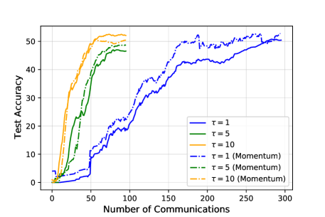
Figure 1: Comparison of the effects of increasing $\tau$ on the performance of Local SGDA and Momentum Local SGDA algorithms, for the fair classification problem on the FashionMNIST dataset, with a VGG11 model. The figure shows the test accuracy for the worst distribution.

We ran the experiment with a VGG11 network. The network has $20$ clients. The data is partitioned across the clients using a Dirichlet distribution $\text{Dir}_{20}(0.1)$ as in Wang et al. (2019), to create a non-iid partitioning of data across clients. We use different values of synchronization frequency $\tau\in\{1,5,10\}$. In accordance with (8), we plot the worst distribution test accuracy in Figure 1. We plot the curves for the number of communications it takes to reach $50\%$ test accuracy on the worst distribution in each case. From Figure 1, we see the communication savings which result from using higher values of $\tau$, since fully synchronized SGDA ($\tau=1$) requires significantly more communication rounds to reach the same accuracy. We also note the superior performance of Momentum Local SGDA, compared to Local SGDA.

5.2 Robust Neural Network Training

Next, we consider the problem of robust neural network (NN) training, in the presence of adversarial perturbations Madry et al. (2018); Sinha et al. (2017). We consider a similar problem as considered in Deng & Mahdavi (2021).

$$\min_{\mathbf{x}}\max_{\left\|{\mathbf{y}}\right\|^{2}\leq 1}\sum_{j=1}^{N}\ell\left(h_{\mathbf{x}}(\mathbf{a}_{i}+{\mathbf{y}}),b_{i}\right),$$ (9)

where ${\mathbf{x}}$ denotes the parameters of the NN, ${\mathbf{y}}$ denotes the perturbation, $(a_{i},b_{i})$ denotes the $i$-th data sample.

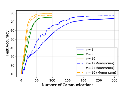
Figure 2: Comparison of the effects of $\tau$ on the performance of Local SGDA and Momentum Local SGDA algorithms, for the robust NN training problem on the CIFAR10 dataset, with the VGG11 model. The figure shows the robust test accuracy.

We ran the experiment using a VGG11 network, with the same network and data partitioning as in the previous subsection. We use different values of $\tau\in\{1,5,10\}$. For both Local SGDA+ and Momentum Local SGDA+, we use $S=\tau^{2}$. In Figure 2, we plot the robust test accuracy. From Figure 2, we see the communication savings which result from using higher values of $\tau$, since for both the algorithms, $\tau=1$ case requires significantly more communication rounds to reach the same accuracy. We also note the superior performance of Momentum Local SGDA+, compared to Local SGDA+ to reach the same accuracy level.

6 Concluding Remarks

In this work, we analyzed existing and newly proposed distributed communication-efficient algorithms for nonconvex minimax optimization problems. We proved order-optimal complexity results, along with communication savings, for several classes of minimax problems. Our results showed linear speedup in the number of clients, which enables scaling up distributed systems. Our results for nonconvex-nonconcave functions improve the existing results for centralized minimax problems. An interesting future direction is to analyze these algorithms for more complex systems with partial and erratic client participation Gu et al. (2021); Ruan et al. (2021), and with a heterogeneous number of local updates at each client Wang et al. (2020).

Appendices

The appendices are organized as follows. In Section A we mention some basic mathematical results and inequalities which are used throughout the paper. In Section B we prove the non-asymptotic convergence of Local SGDA Algorithm 1 for smooth nonconvex-PL (NC-SC) functions, and derive gradient complexity and communication cost of the algorithm to achieve an $\epsilon$-stationary point. In Appendix C, we analyze the proposed Momentum Local SGDA algorithm (Algorithm 2), for the same class of NC-PL functions. Similarly, in the following sections, we prove the non-asymptotic convergence of Algorithm 4 for smooth nonconvex-concave (NC-C) functions (in Appendix D), and for smooth nonconvex-1-point-concave (NC-1PC) functions (in Appendix E). Finally, in Appendix F we provide the details of the additional experiments we performed.

Table 2: Abbreviations for the different classes of minimax problems $\min_{\mathbf{x}}\max_{\mathbf{y}}f({\mathbf{x}},{\mathbf{y}})$ mentioned in the paper.

Function Class	Abbreviation	Our Work
Strongly-Convex in ${\mathbf{x}}$, Strongly-Concave in ${\mathbf{y}}$	SC-SC	-
Strongly-Convex in ${\mathbf{x}}$, Concave in ${\mathbf{y}}$	SC-C	-
Convex in ${\mathbf{x}}$, Concave in ${\mathbf{y}}$	C-C	-
NonConvex in ${\mathbf{x}}$, Strongly-Concave in ${\mathbf{y}}$	NC-SC	(Section 4.1)
NonConvex in ${\mathbf{x}}$ , PL in ${\mathbf{y}}$	NC-PL	(Section 4.1)
NonConvex in ${\mathbf{x}}$ , Concave in ${\mathbf{y}}$	NC-C	(Section 4.2)
NonConvex in ${\mathbf{x}}$, 1-Point-Concave in ${\mathbf{y}}$	NC-1PC	(Section 4.3)
PL in ${\mathbf{x}}$, PL in ${\mathbf{y}}$	PL-PL	-
NonConvex in ${\mathbf{x}}$, Non-Concave in ${\mathbf{y}}$	NC-NC	(Sections 4.1, 4.3)

Appendix A Preliminary Results

Lemma A.1 (Young’s inequality).

Given two same-dimensional vectors $\mathbf{u},\mathbf{v}\in\mathbb{R}^{d}$, the Euclidean inner product can be bounded as follows:

$$\left\langle\mathbf{u},\mathbf{v}\right\rangle\leq\frac{\left\|\mathbf{u}\right\|^{2}}{2\gamma}+\frac{\gamma\left\|\mathbf{v}\right\|^{2}}{2}$$

for every constant $\gamma>0$.

Lemma A.2 (Strong Concavity).

A function $g:\mathcal{X}\times\mathcal{Y}$ is strongly concave in ${\mathbf{y}}$, if there exists a constant $\mu>0$, such that for all ${\mathbf{x}}\in\mathcal{X}$, and for all ${\mathbf{y}},{\mathbf{y}}^{\prime}\in\mathcal{Y}$, the following inequality holds.

$$g({\mathbf{x}},{\mathbf{y}})\leq g({\mathbf{x}},{\mathbf{y}}^{\prime})+\left\langle\nabla_{{\mathbf{y}}}g({\mathbf{x}},{\mathbf{y}}^{\prime}),{\mathbf{y}}^{\prime}-{\mathbf{y}}\right\rangle-\frac{\mu}{2}\left\|{\mathbf{y}}-{\mathbf{y}}^{\prime}\right\|^{2}.$$

Lemma A.3 (Jensen’s inequality).

Given a convex function $f$ and a random variable $X$, the following holds.

$$f\left(\mathbb{E}[X]\right)\leq\mathbb{E}\left[f(X)\right].$$

Lemma A.4 (Sum of squares).

For a positive integer $K$, and a set of vectors $x_{1},\ldots,x_{K}$, the following holds:

$$\left\|\sum_{k=1}^{K}x_{k}\right\|^{2}\leq K\sum_{k=1}^{K}\left\|x_{k}\right\|^{2}.$$

Lemma A.5 (Quadratic growth condition Karimi et al. (2016)).

If function $g$ satisfies Assumptions 1, 4, then for all $x$, the following conditions holds

$$g(x)-\min_{z}g(z) \geq\frac{\mu}{2}\left\|x_{p}-x\right\|^{2},$$

$$\left\|\nabla g(x)\right\|^{2} \geq 2\mu\left(g(x)-\min_{z}g(z)\right).$$

A.1 Local SGD

Local SGD is the algorithm which forms the basis of numerous Federated Learning algorithms Konečnỳ et al. (2016); McMahan et al. (2017). Each client running Local SGD (Algorithm 3), runs a few SGD iterations locally and only then communicates with the server, which in turn computes the average and returns to the clients. This approach saves the limited communication resources of the clients, without sacrificing the convergence guarantees.

The algorithm has been analyzed for both convex and nonconvex minimization problems. With identical distribution of client data, Local SGD has been analyzed in Stich (2018); Stich & Karimireddy (2020); Khaled et al. (2020); Spiridonoff et al. (2021) for (strongly) convex objectives, and in Wang & Joshi (2021); Zhou & Cong (2018) for nonconvex objectives. With heterogeneous client data Local SGD has been analyzed in Khaled et al. (2020); Koloskova et al. (2020) for (strongly) convex objectives, and in Jiang & Agrawal (2018); Haddadpour & Mahdavi (2019); Koloskova et al. (2020) for nonconvex objectives.

Algorithm 3 Local SGD

1:Input: ${\mathbf{x}}_{0}^{i}={\mathbf{x}}_{0}$, for all $i\in[n]$, step-size $\eta$, $\tau$, $T$

2:for $t=0$ to $T-1$ do {At all clients $i=1,\ldots,n$}

3:   Sample minibatch ${\xi^{i}_{t}}$ from local data

4:   ${\mathbf{x}^{i}_{t+1}}={\mathbf{x}^{i}_{t}}-\eta\nabla g_{i}({\mathbf{x}^{i}_{t}};{\xi^{i}_{t}})$

5:   if $t+1$ mod $\tau=0$ then

6:      Clients send $\{{\mathbf{x}^{i}_{t+1}}\}$ to the server

7:      Server computes averages ${\mathbf{x}_{t+1}}\triangleq\frac{1}{n}\sum_{i=1}^{n}{\mathbf{x}^{i}_{t+1}}$, and sends to all the clients

8:      ${\mathbf{x}^{i}_{t+1}}={\mathbf{x}_{t+1}}$, for all $i\in[n]$

9:   end if

10:end for

11:Return: ${\bar{{\mathbf{x}}}_{T}}$ drawn uniformly at random from $\{{\mathbf{x}_{t}}\}$, where ${\mathbf{x}_{t}}\triangleq\frac{1}{n}\sum_{i=1}^{n}{\mathbf{x}^{i}_{t}}$

Lemma A.6 (Local SGD for Convex Function Minimization Khaled et al. (2020)).

Suppose that the local functions $\{g_{i}\}$ satisfy Assumptions 1, 2, 3, and are all convex. Suppose, the step-size $\eta$ is chosen such that $\eta\leq\min\left\{\frac{1}{4L_{f}},\frac{1}{8L_{f}(\tau-1)}\right\}$. Then, the iterates generated by Local SGD (Algorithm 3) algorithm satisfy

$$\mathbb{E}\left[g({\bar{{\mathbf{x}}}_{T}})\right]-g({\mathbf{x}}^{*})\leq\frac{1}{T}\sum_{t=0}^{T-1}\mathbb{E}\left[g({\mathbf{x}_{t}})-g({\mathbf{x}}^{*})\right]\leq\frac{4\left\|{\mathbf{x}}_{0}-{\mathbf{x}}^{*}\right\|^{2}}{\eta T}+\frac{20\eta\sigma^{2}}{n}+16\eta^{2}L_{f}(\tau-1)^{2}\left(\sigma^{2}+\varsigma_{x}^{2}\right),$$

where ${\bar{{\mathbf{x}}}_{T}}\triangleq\frac{1}{T}\sum_{t=0}^{T-1}{\mathbf{x}_{t}}$.

Appendix B Nonconvex-PL (NC-PL) Functions: Local SGDA (Theorem 1)

In this section we prove the convergence of Algorithm 1 for Nonconvex-PL functions, and provide the complexity and communication guarantees.

We organize this section as follows. First, in Section B.1 we present some intermediate results, which we use to prove the main theorem. Next, in Section B.2, we present the proof of Theorem 1, which is followed by the proofs of the intermediate results in Section B.3. We utilize some of the proof techniques of Deng & Mahdavi (2021). However, the algorithm we analyze for NC-PL functions is different. Also, we provide an improved analysis, resulting in better convergence guarantees.

The problem we solve is

$$\min_{{\mathbf{x}}}\max_{{\mathbf{y}}}\left\{f({\mathbf{x}},{\mathbf{y}})\triangleq\frac{1}{n}\sum_{i=1}^{n}f_{i}({\mathbf{x}},{\mathbf{y}})\right\}.$$

We define

$$\Phi({\mathbf{x}})\triangleq\max_{{\mathbf{y}}}f({\mathbf{x}},{\mathbf{y}})\quad\text{and}\quad{\mathbf{y}}^{*}({\mathbf{x}})\in\operatorname*{arg\,max}_{{\mathbf{y}}}f({\mathbf{x}},{\mathbf{y}}).$$ (10)

Since $f({\mathbf{x}},\cdot)$ is $\mu$-PL, ${\mathbf{y}}^{*}({\mathbf{x}})$ need not be unique.

For the sake of analysis, we define virtual sequences of average iterates:

$${\mathbf{x}_{t}}\triangleq\frac{1}{n}\sum_{i=1}^{n}{\mathbf{x}^{i}_{t}};\quad{\mathbf{y}_{t}}\triangleq\frac{1}{n}\sum_{i=1}^{n}{\mathbf{y}^{i}_{t}}.$$

Note that these sequences are constructed only for the sake of analysis. During an actual run of the algorithm, these sequences exist only at the time instants when the clients communicate with the server. We next write the update expressions for these virtual sequences, using the updates in Algorithm 1.

$${\mathbf{x}_{t+1}} ={\mathbf{x}_{t}}-\eta_{x}\frac{1}{n}\sum_{i=1}^{n}\nabla_{{\mathbf{x}}}f_{i}({\mathbf{x}^{i}_{t}},{\mathbf{y}^{i}_{t}};{\xi^{i}_{t}})$$ (11)

$${\mathbf{y}_{t+1}} ={\mathbf{y}_{t}}+\eta_{y}\frac{1}{n}\sum_{i=1}^{n}\nabla_{{\mathbf{y}}}f_{i}({\mathbf{x}^{i}_{t}},{\mathbf{y}^{i}_{t}};{\xi^{i}_{t}})$$

Next, we present some intermediate results which we use in the proof of Theorem 1. To make the proof concise, the proofs of these intermediate results is relegated to Section B.3.

B.1 Intermediate Lemmas

We use the following result from Nouiehed et al. (2019) about the smoothness of $\Phi(\cdot)$.

Lemma B.1.

If the function $f({\mathbf{x}},\cdot)$ satisfies Assumptions 1, 4 ($L_{f}$-smoothness and $\mu$-PL condition in ${\mathbf{y}}$), then $\Phi({\mathbf{x}})$ is $L_{\Phi}$-smooth with $L_{\Phi}=\kappa L/2+L$, where $\kappa=L/\mu$ is the condition number.

Lemma B.2.

Suppose the local client loss functions $\{f_{i}\}$ satisfy Assumptions 1, 4 and the stochastic oracles for the local functions satisfy 2. Then the iterates generated by Algorithm 1 satisfy

$$\mathbb{E}\left[\Phi({\mathbf{x}_{t+1}})\right] \leq\mathbb{E}\left[\Phi({\mathbf{x}_{t}})\right]-\frac{\eta_{x}}{2}\mathbb{E}\left\|\nabla\Phi({\mathbf{x}_{t}})\right\|^{2}-\frac{\eta_{x}}{2}\left(1-L_{\Phi}\eta_{x}\right)\mathbb{E}\left\|\frac{1}{n}\sum_{i=1}^{n}\nabla_{{\mathbf{x}}}f_{i}({\mathbf{x}^{i}_{t}},{\mathbf{y}^{i}_{t}})\right\|^{2}$$

$$\quad+\frac{2\eta_{x}L_{f}^{2}}{\mu}\mathbb{E}\left[\Phi({\mathbf{x}_{t}})-f({\mathbf{x}_{t}},{\mathbf{y}_{t}})\right]+2\eta_{x}L_{f}^{2}\Delta_{t}^{{\mathbf{x}},{\mathbf{y}}}+\frac{L_{\Phi}\eta_{x}^{2}\sigma^{2}}{2n},$$

where, we define $\Delta_{t}^{{\mathbf{x}},{\mathbf{y}}}\triangleq\frac{1}{n}\sum_{i=1}^{n}\mathbb{E}\left(\left\|{\mathbf{x}^{i}_{t}}-{\mathbf{x}_{t}}\right\|^{2}+\left\|{\mathbf{y}^{i}_{t}}-{\mathbf{y}_{t}}\right\|^{2}\right)$, the synchronization error.

Lemma B.3.

Suppose the local loss functions $\{f_{i}\}$ satisfy Assumptions 1, 3, and the stochastic oracles for the local functions satisfy 2. Further, in Algorithm 1, we choose step-sizes $\eta_{x},\eta_{y}$ satisfying $\eta_{y}\leq 1/\mu$, $\frac{\eta_{x}}{\eta_{y}}\leq\frac{1}{8\kappa^{2}}$. Then the following inequality holds.

$$\frac{1}{T}\sum_{t=0}^{T-1}\mathbb{E}\left(\Phi({\mathbf{x}_{t}})-f({\mathbf{x}_{t}},{\mathbf{y}_{t}})\right)$$

$$\leq\frac{2\left(\Phi({\mathbf{x}}_{0})-f({\mathbf{x}}_{0},{\mathbf{y}}_{0})\right)}{\eta_{y}\mu T}+\frac{2L_{f}^{2}}{\mu\eta_{y}}\left(2\eta_{x}(1-\eta_{y}\mu)+\eta_{y}\right)\frac{1}{T}\sum_{t=0}^{T-1}\Delta_{t}^{{\mathbf{x}},{\mathbf{y}}}+(1-\eta_{y}\mu)\frac{\eta_{x}}{\eta_{y}\mu}\frac{1}{T}\sum_{t=0}^{T-1}\mathbb{E}\left\|\nabla\Phi({\mathbf{x}_{t}})\right\|^{2}$$

$$\quad+\left[(1-\eta_{y}\mu)\frac{\eta_{x}^{2}}{2}\left(L_{f}+L_{\Phi}\right)+\eta_{y}L_{f}^{2}\eta_{x}^{2}\right]\frac{2}{\eta_{y}\mu T}\sum_{t=0}^{T-1}\mathbb{E}\left\|\frac{1}{n}\sum_{i=1}^{n}\nabla_{{\mathbf{x}}}f_{i}({\mathbf{x}^{i}_{t}},{\mathbf{y}^{i}_{t}})\right\|^{2}$$

$$\quad+\frac{\sigma^{2}}{\mu n}\left(\eta_{y}L_{f}+2L_{f}^{2}\eta_{x}^{2}\right)+\frac{(1-\eta_{y}\mu)}{\mu\eta_{y}}\frac{\eta_{x}^{2}\sigma^{2}}{n}\left(L_{f}+L_{\Phi}\right).$$

Remark 8 (Comparison with Deng & Mahdavi (2021)).

Note that to derive a result similar to Lemma B.3, the analysis in Deng & Mahdavi (2021) requires the additional assumption of $G_{x}$-Lipschitz continuity of $f(\cdot,{\mathbf{y}})$. Also, the algorithm we analyze (Local SGDA) is simpler than the algorithm analyzed in Deng & Mahdavi (2021) for NC-PL functions.

Lemma B.4.

Suppose the local loss functions $\{f_{i}\}$ satisfy Assumptions 1, 3, and the stochastic oracles for the local functions satisfy 2. Further, in Algorithm 1, we choose step-sizes $\eta_{x},\eta_{y}\leq\frac{1}{8\tau L_{f}}$. Then, the iterates $\{{\mathbf{x}^{i}_{t}},{\mathbf{y}^{i}_{t}}\}$ generated by Algorithm 1 satisfy

$$\frac{1}{T}\sum_{t=0}^{T-1}\Delta_{t}^{{\mathbf{x}},{\mathbf{y}}} \triangleq\frac{1}{T}\sum_{t=0}^{T-1}\frac{1}{n}\sum_{i=1}^{n}\mathbb{E}\left(\left\|{\mathbf{x}^{i}_{t}}-{\mathbf{x}_{t}}\right\|^{2}+\left\|{\mathbf{y}^{i}_{t}}-{\mathbf{y}_{t}}\right\|^{2}\right)$$

$$\leq 2(\tau-1)^{2}\left(\eta_{x}^{2}+\eta_{y}^{2}\right)\sigma^{2}\left(1+\frac{1}{n}\right)+6(\tau-1)^{2}\left(\eta_{x}^{2}\varsigma_{x}^{2}+\eta_{y}^{2}\varsigma_{y}^{2}\right).$$

B.2 Proof of Theorem 1

For the sake of completeness, we first state the full statement of Theorem 1 here.

Theorem.

Suppose the local loss functions $\{f_{i}\}_{i}$ satisfy Assumptions 1, 2, 3, and the global function $f$ satisfies 4. Suppose the step-sizes $\eta_{x},\eta_{y}$ are chosen such that $\eta_{y}\leq\frac{1}{8L_{f}\tau}$, $\frac{\eta_{x}}{\eta_{y}}=\frac{1}{8\kappa^{2}}$, where $\kappa=\frac{L_{f}}{\mu}$ is the condition number. Then for the output ${\bar{{\mathbf{x}}}_{T}}$ of Algorithm 1, the following holds.

$$\mathbb{E}\left\|\nabla\Phi({\bar{{\mathbf{x}}}_{T}})\right\|^{2}= \frac{1}{T}\sum_{t=0}^{T-1}\mathbb{E}\left\|\nabla\Phi({\mathbf{x}_{t}})\right\|^{2}$$

$$\leq\underbrace{\mathcal{O}\left(\kappa^{2}\left[\frac{\Delta_{\Phi}}{\eta_{y}T}+\frac{L_{f}\eta_{y}\sigma^{2}}{n}\right]\right)}_{\text{Error with full synchronization}}+\underbrace{\mathcal{O}\left(L_{f}^{2}\kappa^{2}(\tau-1)^{2}\left[\eta_{y}^{2}\left(\sigma^{2}+\varsigma_{y}^{2}\right)+\eta_{x}^{2}\varsigma_{x}^{2}\right]\right)}_{\text{Error due to local updates}},$$ (12)

where $\Phi({\mathbf{x}})\triangleq\max_{\mathbf{y}}f({\mathbf{x}},{\mathbf{y}})$ is the envelope function, $\Delta_{\Phi}\triangleq\Phi({\mathbf{x}}_{0})-\min_{\mathbf{x}}\Phi({\mathbf{x}})$. Using $\eta_{y}=\sqrt{\frac{n}{L_{f}T}}$ and $\eta_{x}=\frac{1}{8\kappa^{2}}\sqrt{\frac{n}{L_{f}T}}$, we get

$$\mathbb{E}\left\|\nabla\Phi({\bar{{\mathbf{x}}}_{T}})\right\|^{2}\leq\mathcal{O}\left(\frac{\kappa^{2}\left(\sigma^{2}+\Delta_{\Phi}\right)}{\sqrt{nT}}+\kappa^{2}(\tau-1)^{2}\frac{n\left(\sigma^{2}+\varsigma_{x}^{2}+\varsigma_{y}^{2}\right)}{T}\right).$$

Proof.

We start by summing the expression in Lemma B.2 over $t=0,\ldots,T-1$.

$$\frac{1}{T}\sum_{t=0}^{T-1}\mathbb{E}\left[\Phi({\mathbf{x}_{t+1}})-\Phi({\mathbf{x}_{t}})\right] \leq-\frac{\eta_{x}}{2}\frac{1}{T}\sum_{t=0}^{T-1}\mathbb{E}\left\|\nabla\Phi({\mathbf{x}_{t}})\right\|^{2}-\frac{\eta_{x}}{2}\left(1-L_{\Phi}\eta_{x}\right)\frac{1}{T}\sum_{t=0}^{T-1}\mathbb{E}\left\|\frac{1}{n}\sum_{i=1}^{n}\nabla_{{\mathbf{x}}}f_{i}({\mathbf{x}^{i}_{t}},{\mathbf{y}^{i}_{t}})\right\|^{2}$$

$$\quad+\frac{2\eta_{x}L_{f}^{2}}{\mu}\frac{1}{T}\sum_{t=0}^{T-1}\mathbb{E}\left[\Phi({\mathbf{x}_{t}})-F({\mathbf{x}_{t}},{\mathbf{y}_{t}})\right]+2\eta_{x}L_{f}^{2}\frac{1}{T}\sum_{t=0}^{T-1}\Delta_{t}^{{\mathbf{x}},{\mathbf{y}}}+\frac{L_{\Phi}\eta_{x}^{2}\sigma^{2}}{2n}.$$ (13)

Substituting the bound on $\frac{1}{T}\sum_{t=0}^{T-1}\Delta_{t}^{{\mathbf{x}},{\mathbf{y}}}$ from Lemma B.4, and the bound on $\frac{1}{T}\sum_{t=0}^{T-1}\mathbb{E}\left[\Phi({\mathbf{x}_{t}})-F({\mathbf{x}_{t}},{\mathbf{y}_{t}})\right]$ from Lemma B.3, and rearranging the terms in (13), we get

$$\frac{\mathbb{E}\Phi({\mathbf{x}}_{T})-\Phi({\mathbf{x}}_{0})}{T}$$

$$\leq-\underbrace{\left(\frac{\eta_{x}}{2}-(1-\eta_{y}\mu)\frac{2\eta_{x}^{2}L_{f}^{2}}{\eta_{y}\mu^{2}}\right)}_{\geq\eta_{x}/4}\frac{1}{T}\sum_{t=0}^{T-1}\mathbb{E}\left\|\nabla\Phi({\mathbf{x}_{t}})\right\|^{2}$$

$$\quad-\underbrace{\frac{\eta_{x}}{2}\left(1-L_{\Phi}\eta_{x}-\frac{8L_{f}^{2}}{\mu^{2}\eta_{y}}\left[(1-\eta_{y}\mu)\frac{\eta_{x}^{2}}{2}\left(L+L_{\Phi}\right)+\eta_{y}L_{f}^{2}\eta_{x}^{2}\right]\right)}_{\geq 0}\frac{1}{T}\sum_{t=0}^{T-1}\mathbb{E}\left\|\frac{1}{n}\sum_{i=1}^{n}\nabla_{{\mathbf{x}}}f_{i}({\mathbf{x}^{i}_{t}},{\mathbf{y}^{i}_{t}})\right\|^{2}$$

$$\quad+\left[\frac{2\eta_{x}L_{f}^{2}}{\mu}\left(\frac{2L_{f}^{2}}{\mu}+\frac{4\eta_{x}L_{f}^{2}(1-\eta_{y}\mu)}{\mu\eta_{y}}\right)+2\eta_{x}L_{f}^{2}\right]\frac{1}{T}\sum_{t=0}^{T-1}\Delta_{t}^{{\mathbf{x}},{\mathbf{y}}}$$

$$\quad+\frac{2\eta_{x}L_{f}^{2}}{\mu}\left[\frac{2\left(\Phi({\mathbf{x}}_{0})-f({\mathbf{x}}_{0},{\mathbf{y}}_{0})\right)}{\eta_{y}\mu T}+\frac{\sigma^{2}}{\mu n}\left(\eta_{y}L_{f}+2L_{f}^{2}\eta_{x}^{2}\right)+\frac{(1-\eta_{y}\mu)}{\mu\eta_{y}}\frac{\eta_{x}^{2}\sigma^{2}}{n}\left(L_{f}+L_{\Phi}\right)\right]+\frac{L_{\Phi}\eta_{x}^{2}\sigma^{2}}{2n}.$$ (14)

Here, $\frac{\eta_{x}}{2}-\frac{2\eta_{x}^{2}(1-\mu\eta_{y})L_{f}^{2}}{\mu^{2}\eta_{y}}\geq\frac{\eta_{x}}{4}$ holds since $\frac{\eta_{x}}{\eta_{y}}\leq\frac{1}{8\kappa^{2}}$. Also, $1-L_{\Phi}\eta_{x}-\frac{8L_{f}^{2}}{\mu^{2}\eta_{y}}\left[(1-\eta_{y}\mu)\frac{\eta_{x}^{2}}{2}\left(L+L_{\Phi}\right)+\eta_{y}L_{f}^{2}\eta_{x}^{2}\right]\geq 0$ follows from the bounds on $\eta_{x},\eta_{y}$. Rearranging the terms in (14) and using Lemma B.4, we get

$$\frac{1}{T}\sum_{t=0}^{T-1}\mathbb{E}\left\|\nabla\Phi({\mathbf{x}_{t}})\right\|^{2}\leq\frac{4\left(\Phi({\mathbf{x}}_{0})-\mathbb{E}\Phi({\mathbf{x}}_{T})\right)}{\eta_{x}T}$$

$$\quad+\frac{4}{\eta_{x}}2\eta_{x}L_{f}^{2}\left[1+2\kappa^{2}+4\kappa^{2}\frac{\eta_{x}}{\eta_{y}}\right]2(\tau-1)^{2}\left[\left(\eta_{x}^{2}+\eta_{y}^{2}\right)\sigma^{2}\left(1+\frac{1}{n}\right)+3\left(\eta_{x}^{2}\varsigma_{x}^{2}+\eta_{y}^{2}\varsigma_{y}^{2}\right)\right]$$

$$\quad+\frac{4}{\eta_{x}}\left[\frac{4\eta_{x}\kappa^{2}}{\eta_{y}}\frac{\left(\Phi({\mathbf{x}}_{0})-f({\mathbf{x}}_{0},{\mathbf{y}}_{0})\right)}{T}+\frac{2\eta_{x}\kappa^{2}\sigma^{2}}{n}\left(\eta_{y}L_{f}+2L_{f}^{2}\eta_{x}^{2}\right)+\frac{2\eta_{x}\kappa^{2}}{\eta_{y}}\frac{\eta_{x}^{2}\sigma^{2}}{n}\left(L_{f}+L_{\Phi}\right)\right]+\frac{4}{\eta_{x}}\frac{L_{\Phi}\eta_{x}^{2}\sigma^{2}}{2n}$$

$$\overset{(a)}{\leq}\frac{4\Delta_{\Phi}}{\eta_{x}T}+8L_{f}^{2}\left[2+2\kappa^{2}\right]2(\tau-1)^{2}\left[\left(\eta_{x}^{2}+\eta_{y}^{2}\right)\sigma^{2}\left(1+\frac{1}{n}\right)+3\left(\eta_{x}^{2}\varsigma_{x}^{2}+\eta_{y}^{2}\varsigma_{y}^{2}\right)\right]$$

$$\quad+\frac{16\kappa^{2}\Delta_{\Phi}}{\eta_{y}T}+\frac{8\kappa^{2}\sigma^{2}}{n}\left(\eta_{y}L_{f}+2L_{f}^{2}\eta_{x}^{2}\right)+\frac{8\kappa^{2}\eta_{x}}{\eta_{y}}\frac{\eta_{x}\sigma^{2}}{n}\left(L_{f}+L_{\Phi}\right)+\frac{2L_{\Phi}\eta_{x}\sigma^{2}}{n}$$

$$\overset{(b)}{\leq}\frac{4\Delta_{\Phi}}{\eta_{x}T}+192L_{f}^{2}\kappa^{2}(\tau-1)^{2}\left[\left(\eta_{x}^{2}+\eta_{y}^{2}\right)\sigma^{2}+\eta_{x}^{2}\varsigma_{x}^{2}+\eta_{y}^{2}\varsigma_{y}^{2}\right]+\frac{16\kappa^{2}\Delta_{\Phi}}{\eta_{y}T}+\frac{8\kappa^{2}\sigma^{2}}{n}\left(\eta_{y}L_{f}+2L_{f}^{2}\eta_{x}^{2}\right)+\frac{4L_{\Phi}\eta_{x}\sigma^{2}}{n}$$

$$=\mathcal{O}\left(\frac{\Delta_{\Phi}}{\eta_{x}T}+\frac{L_{\Phi}\eta_{x}\sigma^{2}}{n}+\kappa^{2}\left[\frac{\Delta_{\Phi}}{\eta_{y}T}+\frac{L_{f}\eta_{y}\sigma^{2}}{n}\right]+L_{f}^{2}\kappa^{2}(\tau-1)^{2}\left[\left(\eta_{x}^{2}+\eta_{y}^{2}\right)\sigma^{2}+\eta_{x}^{2}\varsigma_{x}^{2}+\eta_{y}^{2}\varsigma_{y}^{2}\right]\right).$$

$$=\underbrace{\mathcal{O}\left(\kappa^{2}\left[\frac{\Delta_{\Phi}}{\eta_{y}T}+\frac{L_{f}\eta_{y}\sigma^{2}}{n}\right]\right)}_{\text{Error with full synchronization}}+\underbrace{\mathcal{O}\left(L_{f}^{2}\kappa^{2}(\tau-1)^{2}\left[\eta_{y}^{2}\left(\sigma^{2}+\varsigma_{y}^{2}\right)+\eta_{x}^{2}\varsigma_{x}^{2}\right]\right)}_{\text{Error due to local updates}}. \because\kappa\geq 1$$ ()

where, we denote $\Delta_{\Phi}\triangleq\Phi({\mathbf{x}}_{0})-\min_{\mathbf{x}}\Phi({\mathbf{x}})$. $(a)$ follows from $\frac{\eta_{x}}{\eta_{y}}\leq\frac{1}{8\kappa^{2}}$; $(b)$ follows since $\kappa\geq 1$ and $L_{\Phi}\geq L_{f}$. Therefore, $\frac{8\kappa^{2}\eta_{x}}{\eta_{y}}\frac{\eta_{x}\sigma^{2}}{n}(L_{f}+L_{\Phi})\leq\frac{\eta_{x}\sigma^{2}}{n}(L_{f}+L_{\Phi})\leq\frac{2L_{\Phi}\eta_{x}\sigma^{2}}{n}$, which results in (12).

Using $\eta_{y}=\sqrt{\frac{n}{L_{f}T}}$ and $\eta_{x}=\frac{1}{8\kappa^{2}}\sqrt{\frac{n}{L_{f}T}}\leq\frac{\eta_{y}}{8\kappa^{2}}$, and since $\kappa\geq 1$, we get

$$\frac{1}{T}\sum_{t=0}^{T-1}\mathbb{E}\left\|\nabla\Phi({\mathbf{x}_{t}})\right\|^{2}\leq\mathcal{O}\left(\frac{\kappa^{2}\left(\sigma^{2}+\Delta_{\Phi}\right)}{\sqrt{nT}}+\kappa^{2}(\tau-1)^{2}\frac{n}{T}\left[\sigma^{2}+\frac{\varsigma_{x}^{2}}{\kappa^{4}}+\varsigma_{y}^{2}\right]\right).$$

∎

Proof of 1.

We assume $T\geq n^{3}$. To reach an $\epsilon$-accurate point, i.e., ${\mathbf{x}}$ such that $\mathbb{E}\left\|\nabla\Phi({\mathbf{x}})\right\|\leq\epsilon$, we need

$$\mathbb{E}\left\|\nabla\Phi({\bar{{\mathbf{x}}}_{T}})\right\|=\left[\frac{1}{T}\sum_{t=0}^{T-1}\mathbb{E}\left\|\nabla\Phi({\mathbf{x}_{t}})\right\|^{2}\right]^{1/2}\leq\mathcal{O}\left(\frac{\kappa\sqrt{\sigma^{2}+\Delta_{\Phi}}}{(nT)^{1/4}}+\kappa(\tau-1)\sqrt{\frac{n\left(\sigma^{2}+\varsigma_{x}^{2}+\varsigma_{y}^{2}\right)}{T}}\right).$$

If we choose $\tau=\mathcal{O}\left(\frac{T^{1/4}}{n^{3/4}}\right)$, we need $T=\mathcal{O}\left(\kappa^{4}/(n\epsilon^{4})\right)$ iterations, to reach an $\epsilon$-accurate point. The number of communication rounds is $\mathcal{O}\left(\frac{T}{\tau}\right)=\mathcal{O}\left((nT)^{3/4}\right)=\mathcal{O}\left(\kappa^{3}/\epsilon^{3}\right)$. ∎

B.3 Proofs of the Intermediate Lemmas

Proof of Lemma B.2.

In the proof, we use the quadratic growth property of $\mu$-PL function $f({\mathbf{x}},\cdot)$ (Lemma A.5), i.e.,

$$\frac{\mu}{2}\left\|{\mathbf{y}}-{\mathbf{y}}^{*}({\mathbf{x}})\right\|^{2}\leq\max_{{\mathbf{y}}^{\prime}}f({\mathbf{x}},{\mathbf{y}}^{\prime})-f({\mathbf{x}},{\mathbf{y}}),\quad\forall\ {\mathbf{x}},{\mathbf{y}}$$ (15)

where ${\mathbf{y}}^{*}({\mathbf{x}})\in\operatorname*{arg\,max}_{{\mathbf{y}}^{\prime}}f({\mathbf{x}},{\mathbf{y}}^{\prime})$. See Deng & Mahdavi (2021) for the entire proof. ∎

Proof of Lemma B.4.

We define the separate synchronization errors for ${\mathbf{x}}$ and ${\mathbf{y}}$

$$\Delta_{t}^{{\mathbf{x}}}\triangleq\frac{1}{n}\sum_{i=1}^{n}\mathbb{E}\left\|{\mathbf{x}^{i}_{t}}-{\mathbf{x}_{t}}\right\|^{2},\qquad\Delta_{t}^{{\mathbf{y}}}\triangleq\frac{1}{n}\sum_{i=1}^{n}\mathbb{E}\left\|{\mathbf{y}^{i}_{t}}-{\mathbf{y}_{t}}\right\|^{2},$$

such that $\Delta_{t}^{{\mathbf{x}},{\mathbf{y}}}=\Delta_{t}^{{\mathbf{x}}}+\Delta_{t}^{{\mathbf{y}}}$. We first bound the ${\mathbf{x}}$- synchronization error $\Delta_{t}^{{\mathbf{x}}}$. Define $s=\lfloor t/\tau\rfloor$, such that $s\tau+1\leq t\leq(s+1)\tau-1$. Then,

$$\Delta_{t}^{{\mathbf{x}}} \triangleq\frac{1}{n}\sum_{i=1}^{n}\mathbb{E}\left\|{\mathbf{x}^{i}_{t}}-{\mathbf{x}_{t}}\right\|^{2}$$

$$=\frac{1}{n}\sum_{i=1}^{n}\mathbb{E}\left\|\Big{(}{\mathbf{x}}^{i}_{s\tau}-\eta_{x}\sum_{k=s\tau}^{t-1}\nabla_{{\mathbf{x}}}f_{i}({\mathbf{x}}_{k}^{i},{\mathbf{y}}_{k}^{i};\xi^{i}_{k})\Big{)}-\Big{(}{\mathbf{x}}_{s\tau}-\eta_{x}\frac{1}{n}\sum_{j=1}^{n}\sum_{k=s\tau}^{t-1}\nabla_{{\mathbf{x}}}f_{j}({\mathbf{x}}_{k}^{j},{\mathbf{y}}_{k}^{j};\xi_{k}^{j})\Big{)}\right\|^{2}$$ (see (11))

$$=\eta_{x}^{2}\frac{1}{n}\sum_{i=1}^{n}\mathbb{E}\left\|\sum_{k=s\tau}^{t-1}\nabla_{{\mathbf{x}}}f_{i}({\mathbf{x}}_{k}^{i},{\mathbf{y}}_{k}^{i};\xi^{i}_{k})-\frac{1}{n}\sum_{j=1}^{n}\sum_{k=s\tau}^{t-1}\nabla_{{\mathbf{x}}}f_{j}({\mathbf{x}}_{k}^{j},{\mathbf{y}}_{k}^{j};\xi_{k}^{j})\right\|^{2} \because{\mathbf{x}}^{i}_{s\tau}={\mathbf{x}}_{s\tau},\forall\ i\in[n]$$ ()

$$\overset{(a)}{\leq}\eta_{x}^{2}\frac{1}{n}(t-s\tau)\sum_{k=s\tau}^{t-1}\sum_{i=1}^{n}\mathbb{E}\Big{\|}\nabla_{{\mathbf{x}}}f_{i}({\mathbf{x}}_{k}^{i},{\mathbf{y}}_{k}^{i};\xi^{i}_{k})-\nabla_{{\mathbf{x}}}f_{i}({\mathbf{x}}_{k}^{i},{\mathbf{y}}_{k}^{i})+\nabla_{{\mathbf{x}}}f_{i}({\mathbf{x}}_{k}^{i},{\mathbf{y}}_{k}^{i})-\nabla_{{\mathbf{x}}}f_{i}({\mathbf{x}}_{k},{\mathbf{y}}_{k})+\nabla_{{\mathbf{x}}}f_{i}({\mathbf{x}}_{k},{\mathbf{y}}_{k})$$

$$\qquad-\nabla_{{\mathbf{x}}}f({\mathbf{x}}_{k},{\mathbf{y}}_{k})-\frac{1}{n}\sum_{j=1}^{n}\left(\nabla_{{\mathbf{x}}}f_{j}({\mathbf{x}}_{k}^{j},{\mathbf{y}}_{k}^{j},\xi_{k}^{j})-\nabla_{{\mathbf{x}}}f_{j}({\mathbf{x}}_{k}^{j},{\mathbf{y}}_{k}^{j})+\nabla_{{\mathbf{x}}}f_{j}({\mathbf{x}}_{k}^{j},{\mathbf{y}}_{k}^{j})-\nabla_{{\mathbf{x}}}f_{j}({\mathbf{x}}_{k},{\mathbf{y}}_{k})\right)\Big{\|}^{2}$$

$$\overset{(b)}{=}\frac{\eta_{x}^{2}(t-s\tau)}{n}\sum_{k=s\tau}^{t-1}\sum_{i=1}^{n}\mathbb{E}\Bigg{[}\left\|\nabla_{{\mathbf{x}}}f_{i}({\mathbf{x}}_{k}^{i},{\mathbf{y}}_{k}^{i};\xi^{i}_{k})-\nabla_{{\mathbf{x}}}f_{i}({\mathbf{x}}_{k}^{i},{\mathbf{y}}_{k}^{i})\right\|^{2}+\Big{\|}\frac{1}{n}\sum_{j=1}^{n}\left(\nabla_{{\mathbf{x}}}f_{j}({\mathbf{x}}_{k}^{j},{\mathbf{y}}_{k}^{j},\xi_{k}^{j})-\nabla_{{\mathbf{x}}}f_{j}({\mathbf{x}}_{k}^{j},{\mathbf{y}}_{k}^{j})\right)\Big{\|}^{2}$$

$$+\Big{\|}\nabla_{{\mathbf{x}}}f_{i}({\mathbf{x}}_{k}^{i},{\mathbf{y}}_{k}^{i})-\nabla_{{\mathbf{x}}}f_{i}({\mathbf{x}}_{k},{\mathbf{y}}_{k})+\nabla_{{\mathbf{x}}}f_{i}({\mathbf{x}}_{k},{\mathbf{y}}_{k})-\nabla_{{\mathbf{x}}}f({\mathbf{x}}_{k},{\mathbf{y}}_{k})-\frac{1}{n}\sum_{j=1}^{n}\left(\nabla_{{\mathbf{x}}}f_{j}({\mathbf{x}}_{k}^{j},{\mathbf{y}}_{k}^{j})-\nabla_{{\mathbf{x}}}f_{j}({\mathbf{x}}_{k},{\mathbf{y}}_{k})\right)\Big{\|}^{2}\Bigg{]}$$

$$\overset{(c)}{\leq}\frac{\eta_{x}^{2}(\tau-1)}{n}\sum_{k=s\tau}^{t-1}\sum_{i=1}^{n}\mathbb{E}\Bigg{[}\sigma^{2}+\frac{\sigma^{2}}{n}+3\left\|\nabla_{{\mathbf{x}}}f_{i}({\mathbf{x}}_{k}^{i},{\mathbf{y}}_{k}^{i})-\nabla_{{\mathbf{x}}}f_{i}({\mathbf{x}}_{k},{\mathbf{y}}_{k})\right\|^{2}+3\left\|\nabla_{{\mathbf{x}}}f_{i}({\mathbf{x}}_{k},{\mathbf{y}}_{k})-\nabla_{{\mathbf{x}}}f({\mathbf{x}}_{k},{\mathbf{y}}_{k})\right\|^{2}$$

$$\qquad\qquad\qquad\qquad\qquad\qquad+3\Big{\|}\frac{1}{n}\sum_{j=1}^{n}\left(\nabla_{{\mathbf{x}}}f_{j}({\mathbf{x}}_{k}^{j},{\mathbf{y}}_{k}^{j})-\nabla_{{\mathbf{x}}}f_{j}({\mathbf{x}}_{k},{\mathbf{y}}_{k})\right)\Big{\|}^{2}\Bigg{]}$$

$$\overset{(d)}{\leq}\frac{\eta_{x}^{2}(\tau-1)}{n}\sum_{k=s\tau}^{t-1}\sum_{i=1}^{n}\mathbb{E}\Bigg{[}\sigma^{2}+\frac{\sigma^{2}}{n}+3L_{f}^{2}\left[\left\|{\mathbf{x}}_{k}^{i}-{\mathbf{x}}_{k}\right\|^{2}+\left\|{\mathbf{y}}_{k}^{i}-{\mathbf{y}}_{k}\right\|^{2}\right]+3\varsigma_{x}^{2}$$

$$\qquad\qquad\qquad\qquad\qquad\qquad+\frac{3}{n}\sum_{j=1}^{n}L_{f}^{2}\left[\left\|{\mathbf{x}}_{k}^{j}-{\mathbf{x}}_{k}\right\|^{2}+\left\|{\mathbf{y}}_{k}^{j}-{\mathbf{y}}_{k}\right\|^{2}\right]\Bigg{]}$$

$$=\eta_{x}^{2}(\tau-1)\sum_{k=s\tau}^{t-1}\left[\sigma^{2}\left(1+\frac{1}{n}\right)+3\varsigma_{x}^{2}+6L_{f}^{2}\left(\Delta_{k}^{{\mathbf{x}}}+\Delta_{k}^{{\mathbf{y}}}\right)\right],$$

where $(a)$ follows from Lemma A.4; $(b)$ follows from 2 (unbiasedness of stochastic gradients); $(c)$ follows from 2 (bounded variance of stochastic gradients); $(d)$ follows from 1, 3, and Jensen’s inequality (Lemma A.3) for $\|\cdot\|^{2}$.

Furthermore, $\Delta_{t}^{{\mathbf{x}}}=0$ for $t=s\tau$. Therefore,

$$\sum_{t=s\tau}^{(s+1)\tau-1}\Delta_{t}^{{\mathbf{x}}}=\sum_{t=s\tau+1}^{(s+1)\tau-1}\Delta_{t}^{{\mathbf{x}}} \leq\eta_{x}^{2}(\tau-1)\sum_{t=s\tau+1}^{(s+1)\tau-1}\sum_{k=s\tau}^{t-1}\left[\sigma^{2}\left(1+\frac{1}{n}\right)+3\varsigma_{x}^{2}+6L_{f}^{2}\left(\Delta_{k}^{{\mathbf{x}}}+\Delta_{k}^{{\mathbf{y}}}\right)\right]$$

$$\leq\eta_{x}^{2}(\tau-1)^{2}\sum_{t=s\tau+1}^{(s+1)\tau-1}\left[\sigma^{2}\left(1+\frac{1}{n}\right)+3\varsigma_{x}^{2}+6L_{f}^{2}\Delta_{t}^{{\mathbf{x}},{\mathbf{y}}}\right].$$ (16)

The ${\mathbf{y}}$- synchronization error $\Delta_{t}^{{\mathbf{y}}}$ following a similar analysis and we get.

$$\sum_{t=s\tau}^{(s+1)\tau-1}\Delta_{t}^{{\mathbf{y}}} \leq\eta_{y}^{2}(\tau-1)^{2}\sum_{t=s\tau+1}^{(s+1)\tau-1}\left[\sigma^{2}\left(1+\frac{1}{n}\right)+3\varsigma_{y}^{2}+6L_{f}^{2}\Delta_{t}^{{\mathbf{x}},{\mathbf{y}}}\right].$$ (17)

Combining (16) and (17), we get

$$\sum_{t=s\tau}^{(s+1)\tau-1}\Delta_{t}^{{\mathbf{x}},{\mathbf{y}}} \leq(\tau-1)^{2}\left[\tau\left(\eta_{x}^{2}+\eta_{y}^{2}\right)\sigma^{2}\left(1+\frac{1}{n}\right)+3\tau\left(\eta_{x}^{2}\varsigma_{x}^{2}+\eta_{y}^{2}\varsigma_{y}^{2}\right)+6L_{f}^{2}\left(\eta_{x}^{2}+\eta_{y}^{2}\right)\sum_{t=s\tau+1}^{(s+1)\tau-1}\Delta_{t}^{{\mathbf{x}},{\mathbf{y}}}\right].$$

Using our choice of $\eta_{x},\eta_{y}$, we have $6L_{f}^{2}\left(\eta_{x}^{2}+\eta_{y}^{2}\right)(\tau-1)^{2}\leq 1/2$, then

$$\sum_{t=s\tau}^{(s+1)\tau-1}\Delta_{t}^{{\mathbf{x}},{\mathbf{y}}} \leq 2\tau(\tau-1)^{2}\left[\left(\eta_{x}^{2}+\eta_{y}^{2}\right)\sigma^{2}\left(1+\frac{1}{n}\right)+3\left(\eta_{x}^{2}\varsigma_{x}^{2}+\eta_{y}^{2}\varsigma_{y}^{2}\right)\right]$$

$$\Rightarrow\frac{1}{T}\sum_{s=0}^{T/\tau-1}\sum_{t=s\tau}^{(s+1)\tau-1}\Delta_{t}^{{\mathbf{x}},{\mathbf{y}}}=\frac{1}{T}\sum_{t=0}^{T-1}\Delta_{t}^{{\mathbf{x}},{\mathbf{y}}} \leq 2(\tau-1)^{2}\left[\left(\eta_{x}^{2}+\eta_{y}^{2}\right)\sigma^{2}\left(1+\frac{1}{n}\right)+3\left(\eta_{x}^{2}\varsigma_{x}^{2}+\eta_{y}^{2}\varsigma_{y}^{2}\right)\right].$$

∎

Proof of Lemma B.3.

Using $L_{f}$-smoothness of $f({\mathbf{x}},\cdot)$,

$$f({\mathbf{x}_{t+1}},{\mathbf{y}_{t}}) +\left\langle\nabla_{{\mathbf{y}}}f({\mathbf{x}_{t+1}},{\mathbf{y}_{t}}),{\mathbf{y}_{t+1}}-{\mathbf{y}_{t}}\right\rangle-\frac{L_{f}}{2}\left\|{\mathbf{y}_{t+1}}-{\mathbf{y}_{t}}\right\|^{2}\leq f({\mathbf{x}_{t+1}},{\mathbf{y}_{t+1}})$$

$$\Rightarrow f({\mathbf{x}_{t+1}},{\mathbf{y}_{t}}) \leq f({\mathbf{x}_{t+1}},{\mathbf{y}_{t+1}})-\eta_{y}\left\langle\nabla_{{\mathbf{y}}}f({\mathbf{x}_{t+1}},{\mathbf{y}_{t}}),\frac{1}{n}\sum_{i=1}^{n}\nabla_{{\mathbf{y}}}f_{i}({\mathbf{x}^{i}_{t}},{\mathbf{y}^{i}_{t}};{\xi^{i}_{t}})\right\rangle+\frac{\eta_{y}^{2}L_{f}}{2}\left\|\frac{1}{n}\sum_{i=1}^{n}\nabla_{{\mathbf{y}}}f_{i}({\mathbf{x}^{i}_{t}},{\mathbf{y}^{i}_{t}};{\xi^{i}_{t}})\right\|^{2}$$ (using (11))

$$\Rightarrow\mathbb{E}f({\mathbf{x}_{t+1}},{\mathbf{y}_{t}}) \leq\mathbb{E}f({\mathbf{x}_{t+1}},{\mathbf{y}_{t+1}})-\eta_{y}\mathbb{E}\left\langle\nabla_{{\mathbf{y}}}f({\mathbf{x}_{t+1}},{\mathbf{y}_{t}}),\frac{1}{n}\sum_{i=1}^{n}\nabla_{{\mathbf{y}}}f_{i}({\mathbf{x}^{i}_{t}},{\mathbf{y}^{i}_{t}})\right\rangle$$

$$\qquad+\frac{\eta_{y}^{2}L_{f}}{2}\left[\frac{\sigma^{2}}{n}+\left\|\frac{1}{n}\sum_{i=1}^{n}\nabla_{{\mathbf{y}}}f_{i}({\mathbf{x}^{i}_{t}},{\mathbf{y}^{i}_{t}})\right\|^{2}\right]$$ (2)

$$=\mathbb{E}f({\mathbf{x}_{t+1}},{\mathbf{y}_{t+1}})-\frac{\eta_{y}}{2}\mathbb{E}\left\|\nabla_{{\mathbf{y}}}f({\mathbf{x}_{t+1}},{\mathbf{y}_{t}})\right\|^{2}-\frac{\eta_{y}}{2}\left(1-\eta_{y}L_{f}\right)\mathbb{E}\left\|\frac{1}{n}\sum_{i=1}^{n}\nabla_{{\mathbf{y}}}f_{i}({\mathbf{x}^{i}_{t}},{\mathbf{y}^{i}_{t}})\right\|^{2}$$

$$\qquad+\frac{\eta_{y}}{2}\mathbb{E}\left\|\nabla_{{\mathbf{y}}}f({\mathbf{x}_{t+1}},{\mathbf{y}_{t}})-\nabla_{{\mathbf{y}}}f({\mathbf{x}_{t}},{\mathbf{y}_{t}})+\nabla_{{\mathbf{y}}}f({\mathbf{x}_{t}},{\mathbf{y}_{t}})-\frac{1}{n}\sum_{i=1}^{n}\nabla_{{\mathbf{y}}}f_{i}({\mathbf{x}^{i}_{t}},{\mathbf{y}^{i}_{t}})\right\|^{2}+\frac{\eta_{y}^{2}L_{f}\sigma^{2}}{2n}$$

$$\leq\mathbb{E}f({\mathbf{x}_{t+1}},{\mathbf{y}_{t+1}})-\frac{\eta_{y}}{2}\mathbb{E}\left\|\nabla_{{\mathbf{y}}}f({\mathbf{x}_{t+1}},{\mathbf{y}_{t}})\right\|^{2}-\frac{\eta_{y}}{2}\left(1-\eta_{y}L_{f}\right)\mathbb{E}\left\|\frac{1}{n}\sum_{i=1}^{n}\nabla_{{\mathbf{y}}}f_{i}({\mathbf{x}^{i}_{t}},{\mathbf{y}^{i}_{t}})\right\|^{2}$$

$$\qquad+\eta_{y}L_{f}^{2}\mathbb{E}\left\|{\mathbf{x}_{t+1}}-{\mathbf{x}_{t}}\right\|^{2}+\eta_{y}L_{f}^{2}\Delta_{t}^{{\mathbf{x}},{\mathbf{y}}}+\frac{\eta_{y}^{2}L_{f}\sigma^{2}}{2n},$$ (18)

where (18) follows from Jensen’s inequality (Lemma A.3) for $\left\|\cdot\right\|^{2}$, 1 and Young’s inequality (Lemma A.1) for $\gamma=1$, $\left\langle\mathbf{a},\bf b\right\rangle\leq\frac{1}{2}\left\|\mathbf{a}\right\|^{2}+\frac{1}{2}\left\|\mathbf{b}\right\|^{2}$. Next, note that using 2

$$\mathbb{E}\left\|{\mathbf{x}_{t+1}}-{\mathbf{x}_{t}}\right\|^{2} =\eta_{x}^{2}\mathbb{E}\left\|\frac{1}{n}\sum_{i=1}^{n}\nabla_{{\mathbf{x}}}f_{i}({\mathbf{x}^{i}_{t}},{\mathbf{y}^{i}_{t}};{\xi^{i}_{t}})\right\|^{2}\leq\eta_{x}^{2}\left\|\frac{1}{n}\sum_{i=1}^{n}\nabla_{{\mathbf{x}}}f_{i}({\mathbf{x}^{i}_{t}},{\mathbf{y}^{i}_{t}})\right\|^{2}+\frac{\eta_{x}^{2}\sigma^{2}}{n}.$$ (19)

Also, using 4,

$$\left\|\nabla_{{\mathbf{y}}}f({\mathbf{x}_{t+1}},{\mathbf{y}_{t}})\right\|^{2}\geq 2\mu\left(\max_{\mathbf{y}}f({\mathbf{x}_{t+1}},{\mathbf{y}})-f({\mathbf{x}_{t+1}},{\mathbf{y}_{t}})\right)=2\mu\left(\Phi({\mathbf{x}_{t+1}})-f({\mathbf{x}_{t+1}},{\mathbf{y}_{t}})\right).$$ (20)

Substituting (19), (20) in (18), and rearranging the terms, we get

$$\eta_{y}\mu\mathbb{E}\left(\Phi({\mathbf{x}_{t+1}})-f({\mathbf{x}_{t+1}},{\mathbf{y}_{t}})\right)$$

$$\leq\mathbb{E}f({\mathbf{x}_{t+1}},{\mathbf{y}_{t+1}})-\mathbb{E}f({\mathbf{x}_{t+1}},{\mathbf{y}_{t}})-\frac{\eta_{y}}{2}\left(1-\eta_{y}L_{f}\right)\mathbb{E}\left\|\frac{1}{n}\sum_{i=1}^{n}\nabla_{{\mathbf{y}}}f_{i}({\mathbf{x}^{i}_{t}},{\mathbf{y}^{i}_{t}})\right\|^{2}+\frac{\eta_{y}^{2}L_{f}\sigma^{2}}{2n}$$

$$\quad+\eta_{y}L_{f}^{2}\left[\eta_{x}^{2}\mathbb{E}\left\|\frac{1}{n}\sum_{i=1}^{n}\nabla_{{\mathbf{x}}}f_{i}({\mathbf{x}^{i}_{t}},{\mathbf{y}^{i}_{t}})\right\|^{2}+\frac{\eta_{x}^{2}\sigma^{2}}{n}\right]+\eta_{y}L_{f}^{2}\Delta_{t}^{{\mathbf{x}},{\mathbf{y}}}$$

$$\Rightarrow \mathbb{E}\left(\Phi({\mathbf{x}_{t+1}})-f({\mathbf{x}_{t+1}},{\mathbf{y}_{t+1}})\right)$$

$$\leq(1-\eta_{y}\mu)\mathbb{E}\left(\Phi({\mathbf{x}_{t+1}})-f({\mathbf{x}_{t+1}},{\mathbf{y}_{t}})\right)-\frac{\eta_{y}}{2}\left(1-\eta_{y}L_{f}\right)\mathbb{E}\left\|\frac{1}{n}\sum_{i=1}^{n}\nabla_{{\mathbf{y}}}f_{i}({\mathbf{x}^{i}_{t}},{\mathbf{y}^{i}_{t}})\right\|^{2}+\frac{\eta_{y}^{2}L_{f}\sigma^{2}}{2n}$$

$$\quad+\eta_{y}L_{f}^{2}\left[\eta_{x}^{2}\mathbb{E}\left\|\frac{1}{n}\sum_{i=1}^{n}\nabla_{{\mathbf{x}}}f_{i}({\mathbf{x}^{i}_{t}},{\mathbf{y}^{i}_{t}})\right\|^{2}+\frac{\eta_{x}^{2}\sigma^{2}}{n}\right]+\eta_{y}L_{f}^{2}\Delta_{t}^{{\mathbf{x}},{\mathbf{y}}}.$$ (21)

Next, we bound $\mathbb{E}\left(\Phi({\mathbf{x}_{t+1}})-f({\mathbf{x}_{t+1}},{\mathbf{y}_{t}})\right)$.

$$\mathbb{E}\left[\Phi({\mathbf{x}_{t+1}})-f({\mathbf{x}_{t+1}},{\mathbf{y}_{t}})\right]$$

$$=\underbrace{\mathbb{E}\left[\Phi({\mathbf{x}_{t+1}})-\Phi({\mathbf{x}_{t}})\right]}_{I_{1}}+\mathbb{E}\left[\Phi({\mathbf{x}_{t}})-f({\mathbf{x}_{t}},{\mathbf{y}_{t}})\right]+\underbrace{\mathbb{E}\left[f({\mathbf{x}_{t}},{\mathbf{y}_{t}})-f({\mathbf{x}_{t+1}},{\mathbf{y}_{t}})\right]}_{I_{2}}$$ (22)

$I_{1}$ is bounded in Lemma B.2. We next bound $I_{2}$. Using $L_{f}$-smoothness of $f(\cdot,{\mathbf{y}_{t}})$,

$$f({\mathbf{x}_{t}},{\mathbf{y}_{t}})+\left\langle\nabla_{{\mathbf{x}}}f({\mathbf{x}_{t}},{\mathbf{y}_{t}}),{\mathbf{x}_{t+1}}-{\mathbf{x}_{t}}\right\rangle-\frac{L_{f}}{2}\left\|{\mathbf{x}_{t+1}}-{\mathbf{x}_{t}}\right\|^{2}\leq f({\mathbf{x}_{t+1}},{\mathbf{y}_{t}})$$

$$\Rightarrow I_{2} =\mathbb{E}\left[f({\mathbf{x}_{t}},{\mathbf{y}_{t}})-f({\mathbf{x}_{t+1}},{\mathbf{y}_{t}})\right]$$

$$\leq\eta_{x}\mathbb{E}\left\langle\nabla_{{\mathbf{x}}}f({\mathbf{x}_{t}},{\mathbf{y}_{t}}),\frac{1}{n}\sum_{i=1}^{n}\nabla_{{\mathbf{x}}}f_{i}({\mathbf{x}^{i}_{t}},{\mathbf{y}^{i}_{t}};{\xi^{i}_{t}})\right\rangle+\frac{\eta_{x}^{2}L_{f}}{2}\mathbb{E}\left\|\frac{1}{n}\sum_{i=1}^{n}\nabla_{{\mathbf{x}}}f_{i}({\mathbf{x}^{i}_{t}},{\mathbf{y}^{i}_{t}};{\xi^{i}_{t}})\right\|^{2}$$

$$\leq\eta_{x}\mathbb{E}\left\langle\nabla_{{\mathbf{x}}}f({\mathbf{x}_{t}},{\mathbf{y}_{t}}),\frac{1}{n}\sum_{i=1}^{n}\nabla_{{\mathbf{x}}}f_{i}({\mathbf{x}^{i}_{t}},{\mathbf{y}^{i}_{t}})\right\rangle+\frac{\eta_{x}^{2}L_{f}}{2}\left[\frac{\sigma^{2}}{n}+\mathbb{E}\left\|\frac{1}{n}\sum_{i=1}^{n}\nabla_{{\mathbf{x}}}f_{i}({\mathbf{x}^{i}_{t}},{\mathbf{y}^{i}_{t}})\right\|^{2}\right]$$ (2)

$$\leq\frac{\eta_{x}}{2}\mathbb{E}\left[\left\|\nabla_{{\mathbf{x}}}f({\mathbf{x}_{t}},{\mathbf{y}_{t}})\right\|^{2}+\left\|\frac{1}{n}\sum_{i=1}^{n}\nabla_{{\mathbf{x}}}f_{i}({\mathbf{x}^{i}_{t}},{\mathbf{y}^{i}_{t}})\right\|^{2}\right]+\frac{\eta_{x}^{2}L_{f}}{2}\left[\frac{\sigma^{2}}{n}+\mathbb{E}\left\|\frac{1}{n}\sum_{i=1}^{n}\nabla_{{\mathbf{x}}}f_{i}({\mathbf{x}^{i}_{t}},{\mathbf{y}^{i}_{t}})\right\|^{2}\right]$$

$$\leq\eta_{x}\mathbb{E}\left[\left\|\nabla\Phi({\mathbf{x}_{t}})\right\|^{2}+\left\|\nabla_{{\mathbf{x}}}f({\mathbf{x}_{t}},{\mathbf{y}_{t}})-\nabla\Phi({\mathbf{x}_{t}})\right\|^{2}\right]+\frac{\eta_{x}^{2}L_{f}\sigma^{2}}{2n}+\frac{\eta_{x}}{2}\left(1+\eta_{x}L_{f}\right)\mathbb{E}\left\|\frac{1}{n}\sum_{i=1}^{n}\nabla_{{\mathbf{x}}}f_{i}({\mathbf{x}^{i}_{t}},{\mathbf{y}^{i}_{t}})\right\|^{2}$$

$$\overset{(a)}{\leq}\eta_{x}\mathbb{E}\left\|\nabla\Phi({\mathbf{x}_{t}})\right\|^{2}+\eta_{x}L_{f}^{2}\mathbb{E}\left\|{\mathbf{y}_{t}}-{\mathbf{y}}^{*}({\mathbf{x}_{t}})\right\|^{2}+\frac{\eta_{x}^{2}L_{f}\sigma^{2}}{2n}+\frac{\eta_{x}}{2}\left(1+\eta_{x}L_{f}\right)\mathbb{E}\left\|\frac{1}{n}\sum_{i=1}^{n}\nabla_{{\mathbf{x}}}f_{i}({\mathbf{x}^{i}_{t}},{\mathbf{y}^{i}_{t}})\right\|^{2}$$

$$\leq\eta_{x}\mathbb{E}\left\|\nabla\Phi({\mathbf{x}_{t}})\right\|^{2}+\frac{2\eta_{x}L_{f}^{2}}{\mu}\mathbb{E}\left[\Phi({\mathbf{x}_{t}})-f({\mathbf{x}_{t}},{\mathbf{y}_{t}})\right]+\frac{\eta_{x}^{2}L_{f}\sigma^{2}}{2n}+\frac{\eta_{x}}{2}\left(1+\eta_{x}L_{f}\right)\mathbb{E}\left\|\frac{1}{n}\sum_{i=1}^{n}\nabla_{{\mathbf{x}}}f_{i}({\mathbf{x}^{i}_{t}},{\mathbf{y}^{i}_{t}})\right\|^{2}.$$ (23)

where $(a)$ follows from 1 and Lemma B.1. Also, recall that ${\mathbf{y}}^{*}({\mathbf{x}})\in\operatorname*{arg\,max}_{{\mathbf{y}}^{\prime}}f({\mathbf{x}},{\mathbf{y}}^{\prime})$. (23) follows from the quadratic growth property of $\mu$-PL functions (Lemma A.5). Substituting the bounds on $I_{1},I_{2}$ from Lemma B.2 and (23) respectively, in (21), we get

$$\mathbb{E}\left(\Phi({\mathbf{x}_{t+1}})-f({\mathbf{x}_{t+1}},{\mathbf{y}_{t+1}})\right)$$

$$\leq(1-\eta_{y}\mu)\left(1+\frac{4\eta_{x}L_{f}^{2}}{\mu}\right)\mathbb{E}\left(\Phi({\mathbf{x}_{t}})-f({\mathbf{x}_{t}},{\mathbf{y}_{t}})\right)$$

$$\quad+(1-\eta_{y}\mu)\left[-\frac{\eta_{x}}{2}\mathbb{E}\left\|\nabla\Phi({\mathbf{x}_{t}})\right\|^{2}-\frac{\eta_{x}}{2}\left(1-L_{\Phi}\eta_{x}\right)\mathbb{E}\left\|\frac{1}{n}\sum_{i=1}^{n}\nabla_{{\mathbf{x}}}f_{i}({\mathbf{x}^{i}_{t}},{\mathbf{y}^{i}_{t}})\right\|^{2}+2\eta_{x}L_{f}^{2}\Delta_{t}^{{\mathbf{x}},{\mathbf{y}}}+\frac{L_{\Phi}\eta_{x}^{2}\sigma^{2}}{2n}\right]$$

$$\quad+(1-\eta_{y}\mu)\left[\eta_{x}\mathbb{E}\left\|\nabla\Phi({\mathbf{x}_{t}})\right\|^{2}+\frac{\eta_{x}^{2}L_{f}\sigma^{2}}{2n}+\frac{\eta_{x}}{2}\left(1+\eta_{x}L_{f}\right)\mathbb{E}\left\|\frac{1}{n}\sum_{i=1}^{n}\nabla_{{\mathbf{x}}}f_{i}({\mathbf{x}^{i}_{t}},{\mathbf{y}^{i}_{t}})\right\|^{2}\right]$$

$$\quad-\frac{\eta_{y}}{2}\left(1-\eta_{y}L_{f}\right)\mathbb{E}\left\|\frac{1}{n}\sum_{i=1}^{n}\nabla_{{\mathbf{y}}}f_{i}({\mathbf{x}^{i}_{t}},{\mathbf{y}^{i}_{t}})\right\|^{2}+\frac{\eta_{y}^{2}L_{f}\sigma^{2}}{2n}$$

$$\quad+\eta_{y}L_{f}^{2}\left[\eta_{x}^{2}\left\|\frac{1}{n}\sum_{i=1}^{n}\nabla_{{\mathbf{x}}}f_{i}({\mathbf{x}^{i}_{t}},{\mathbf{y}^{i}_{t}})\right\|^{2}+\frac{\eta_{x}^{2}\sigma^{2}}{n}\right]+\eta_{y}L_{f}^{2}\Delta_{t}^{{\mathbf{x}},{\mathbf{y}}}$$

$$\leq\left(1-\frac{\eta_{y}\mu}{2}\right)\mathbb{E}\left(\Phi({\mathbf{x}_{t}})-f({\mathbf{x}_{t}},{\mathbf{y}_{t}})\right)+\frac{\eta_{y}^{2}L_{f}\sigma^{2}}{2n}+\frac{\eta_{y}L_{f}^{2}\eta_{x}^{2}\sigma^{2}}{n}+\eta_{y}L_{f}^{2}\Delta_{t}^{{\mathbf{x}},{\mathbf{y}}}$$

$$\quad+\left[(1-\eta_{y}\mu)\frac{\eta_{x}^{2}}{2}\left(L_{f}+L_{\Phi}\right)+\eta_{y}L_{f}^{2}\eta_{x}^{2}\right]\mathbb{E}\left\|\frac{1}{n}\sum_{i=1}^{n}\nabla_{{\mathbf{x}}}f_{i}({\mathbf{x}^{i}_{t}},{\mathbf{y}^{i}_{t}})\right\|^{2}$$

$$\quad+(1-\eta_{y}\mu)\left[\frac{\eta_{x}}{2}\mathbb{E}\left\|\nabla\Phi({\mathbf{x}_{t}})\right\|^{2}+\frac{\eta_{x}^{2}L_{f}\sigma^{2}}{2n}+2\eta_{x}L_{f}^{2}\Delta_{t}^{{\mathbf{x}},{\mathbf{y}}}+\frac{L_{\Phi}\eta_{x}^{2}\sigma^{2}}{2n}\right],$$ (24)

where we choose $\eta_{x}$ such that $(1-\eta_{y}\mu)\left(1+\frac{4\eta_{x}L_{f}^{2}}{\mu}\right)\leq\left(1-\frac{\eta_{y}\mu}{2}\right)$. This holds if $\frac{4\eta_{x}L_{f}^{2}}{\mu}\leq\frac{\eta_{y}\mu}{2}\Rightarrow\eta_{x}\leq\frac{\eta_{y}}{8\kappa^{2}}$. Summing (24) over $t=0,\ldots,T-1$, and rearranging the terms, we get

$$\frac{1}{T}\sum_{t=0}^{T-1}\mathbb{E}\left(\Phi({\mathbf{x}_{t+1}})-f({\mathbf{x}_{t+1}},{\mathbf{y}_{t+1}})\right)$$

$$\leq\left(1-\frac{\eta_{y}\mu}{2}\right)\frac{1}{T}\sum_{t=0}^{T-1}\mathbb{E}\left(\Phi({\mathbf{x}_{t}})-f({\mathbf{x}_{t}},{\mathbf{y}_{t}})\right)+L_{f}^{2}\left(2\eta_{x}(1-\eta_{y}\mu)+\eta_{y}\right)\frac{1}{T}\sum_{t=0}^{T-1}\Delta_{t}^{{\mathbf{x}},{\mathbf{y}}}$$

$$\quad+\left[(1-\eta_{y}\mu)\frac{\eta_{x}^{2}}{2}\left(L_{f}+L_{\Phi}\right)+\eta_{y}L_{f}^{2}\eta_{x}^{2}\right]\frac{1}{T}\sum_{t=0}^{T-1}\mathbb{E}\left\|\frac{1}{n}\sum_{i=1}^{n}\nabla_{{\mathbf{x}}}f_{i}({\mathbf{x}^{i}_{t}},{\mathbf{y}^{i}_{t}})\right\|^{2}+(1-\eta_{y}\mu)\frac{\eta_{x}}{2}\frac{1}{T}\sum_{t=0}^{T-1}\mathbb{E}\left\|\nabla\Phi({\mathbf{x}_{t}})\right\|^{2}$$

$$\quad+\frac{\eta_{y}^{2}L_{f}\sigma^{2}}{2n}+\frac{\eta_{y}L_{f}^{2}\eta_{x}^{2}\sigma^{2}}{n}+(1-\eta_{y}\mu)\left[\frac{\eta_{x}^{2}L_{f}\sigma^{2}}{2n}+\frac{L_{\Phi}\eta_{x}^{2}\sigma^{2}}{2n}\right].$$

Rearranging the terms, we get

$$\frac{1}{T}\sum_{t=0}^{T-1}\mathbb{E}\left(\Phi({\mathbf{x}_{t}})-f({\mathbf{x}_{t}},{\mathbf{y}_{t}})\right)$$

$$\leq\frac{2}{\eta_{y}\mu}\left[\frac{\Phi({\mathbf{x}}_{0})-f({\mathbf{x}}_{0},{\mathbf{y}}_{0})}{T}-\frac{\mathbb{E}\left(\Phi({\mathbf{x}}_{T})-f({\mathbf{x}}_{T},{\mathbf{y}}_{T})\right)}{T}\right]+\frac{2L_{f}^{2}}{\mu\eta_{y}}\left(2\eta_{x}(1-\eta_{y}\mu)+\eta_{y}\right)\frac{1}{T}\sum_{t=0}^{T-1}\Delta_{t}^{{\mathbf{x}},{\mathbf{y}}}$$

$$\quad+\left[(1-\eta_{y}\mu)\frac{\eta_{x}^{2}}{2}\left(L_{f}+L_{\Phi}\right)+\eta_{y}L_{f}^{2}\eta_{x}^{2}\right]\frac{2}{\eta_{y}\mu T}\sum_{t=0}^{T-1}\mathbb{E}\left\|\frac{1}{n}\sum_{i=1}^{n}\nabla_{{\mathbf{x}}}f_{i}({\mathbf{x}^{i}_{t}},{\mathbf{y}^{i}_{t}})\right\|^{2}+(1-\eta_{y}\mu)\frac{\eta_{x}}{\eta_{y}\mu T}\sum_{t=0}^{T-1}\mathbb{E}\left\|\nabla\Phi({\mathbf{x}_{t}})\right\|^{2}$$

$$\quad+\frac{\eta_{y}L_{f}\sigma^{2}}{\mu n}+\frac{2L_{f}^{2}\eta_{x}^{2}\sigma^{2}}{\mu n}+\frac{(1-\eta_{y}\mu)}{\mu\eta_{y}}\left[\frac{\eta_{x}^{2}L_{f}\sigma^{2}}{n}+\frac{L_{\Phi}\eta_{x}^{2}\sigma^{2}}{n}\right]$$

$$\leq\frac{2\left(\Phi({\mathbf{x}}_{0})-f({\mathbf{x}}_{0},{\mathbf{y}}_{0})\right)}{\eta_{y}\mu T}+\frac{2L_{f}^{2}}{\mu\eta_{y}}\left(2\eta_{x}(1-\eta_{y}\mu)+\eta_{y}\right)\frac{1}{T}\sum_{t=0}^{T-1}\Delta_{t}^{{\mathbf{x}},{\mathbf{y}}} \because\Phi({\mathbf{x}}_{T})\triangleq\operatorname*{arg\,max}_{\mathbf{y}}f({\mathbf{x}}_{T},{\mathbf{y}})$$ ()

$$\quad+\left[(1-\eta_{y}\mu)\frac{\eta_{x}^{2}}{2}\left(L_{f}+L_{\Phi}\right)+\eta_{y}L_{f}^{2}\eta_{x}^{2}\right]\frac{2}{\eta_{y}\mu T}\sum_{t=0}^{T-1}\mathbb{E}\left\|\frac{1}{n}\sum_{i=1}^{n}\nabla_{{\mathbf{x}}}f_{i}({\mathbf{x}^{i}_{t}},{\mathbf{y}^{i}_{t}})\right\|^{2}+(1-\eta_{y}\mu)\frac{\eta_{x}}{\eta_{y}\mu T}\sum_{t=0}^{T-1}\mathbb{E}\left\|\nabla\Phi({\mathbf{x}_{t}})\right\|^{2}$$

$$\quad+\frac{\eta_{y}L_{f}\sigma^{2}}{\mu n}+\frac{2L_{f}^{2}\eta_{x}^{2}\sigma^{2}}{\mu n}+\frac{(1-\eta_{y}\mu)}{\mu\eta_{y}}\left[\frac{\eta_{x}^{2}L_{f}\sigma^{2}}{n}+\frac{L_{\Phi}\eta_{x}^{2}\sigma^{2}}{n}\right],$$

which concludes the proof. ∎

Appendix C Nonconvex-PL (NC-PL) Functions: Momentum Local SGDA (Theorem 2)

In this section we prove the convergence of Algorithm 2 for Nonconvex-PL functions, and provide the complexity and communication guarantees.

We organize this section as follows. First, in Section C.1 we present some intermediate results. Next, in Section C.2, we present the proof of Theorem 2, which is followed by the proofs of the intermediate results in Section C.3.

Again, the problem we solve is

$$\min_{{\mathbf{x}}}\max_{{\mathbf{y}}}\left\{f({\mathbf{x}},{\mathbf{y}})\triangleq\frac{1}{n}\sum_{i=1}^{n}f_{i}({\mathbf{x}},{\mathbf{y}})\right\}.$$

We define

$$\Phi({\mathbf{x}})\triangleq\max_{{\mathbf{y}}}f({\mathbf{x}},{\mathbf{y}})\quad\text{and}\quad{\mathbf{y}}^{*}({\mathbf{x}})\in\operatorname*{arg\,max}_{{\mathbf{y}}}f({\mathbf{x}},{\mathbf{y}}).$$ (25)

Since $f({\mathbf{x}},\cdot)$ is $\mu$-PL (4), ${\mathbf{y}}^{*}({\mathbf{x}})$ is not necessarily unique.

For the sake of analysis, we define virtual sequences of average iterates and average direction estimates:

$${\mathbf{x}_{t}}\triangleq\frac{1}{n}\sum_{i=1}^{n}{\mathbf{x}^{i}_{t}};\quad{\mathbf{y}_{t}}\triangleq\frac{1}{n}\sum_{i=1}^{n}{\mathbf{y}^{i}_{t}};$$

$$\widetilde{{\mathbf{x}}}_{t+\frac{1}{2}}\triangleq\frac{1}{n}\sum_{i=1}^{n}\widetilde{{\mathbf{x}}}^{i}_{t+\frac{1}{2}};\quad\tilde{{\mathbf{y}}}_{t+\frac{1}{2}}\triangleq\frac{1}{n}\sum_{i=1}^{n}\tilde{{\mathbf{y}}}^{i}_{t+\frac{1}{2}};$$

$${\mathbf{d}_{x,t}}\triangleq\frac{1}{n}\sum_{i=1}^{n}{\mathbf{d}^{i}_{x,t}};\quad{\mathbf{d}_{y,t}}\triangleq\frac{1}{n}\sum_{i=1}^{n}{\mathbf{d}^{i}_{y,t}}.$$

Note that these sequences are constructed only for the sake of analysis. During an actual run of the algorithm, these sequences exist only at the time instants when the clients communicate with the server. We next write the update expressions for these virtual sequences, using the updates in Algorithm 2.

$$\widetilde{{\mathbf{x}}}_{t+\frac{1}{2}}={\mathbf{x}_{t}}-\eta_{x}{\mathbf{d}_{x,t}},\qquad{\mathbf{x}_{t+1}}={\mathbf{x}_{t}}+\alpha_{t}\left(\widetilde{{\mathbf{x}}}_{t+\frac{1}{2}}-{\mathbf{x}_{t}}\right)$$ (26)

$$\tilde{{\mathbf{y}}}_{t+\frac{1}{2}}={\mathbf{y}_{t}}+\eta_{y}{\mathbf{d}_{y,t}},\qquad{\mathbf{y}_{t+1}}={\mathbf{y}_{t}}+\alpha_{t}\left(\tilde{{\mathbf{y}}}_{t+\frac{1}{2}}-{\mathbf{y}_{t}}\right)$$

$${\mathbf{d}_{x,t+1}}=(1-\beta_{x}\alpha_{t}){\mathbf{d}_{x,t}}+\beta_{x}\alpha_{t}\frac{1}{n}\sum_{i=1}^{n}\nabla_{{\mathbf{x}}}f_{i}({\mathbf{x}^{i}_{t+1}},{\mathbf{y}^{i}_{t+1}};{\xi^{i}_{t+1}})$$

$${\mathbf{d}_{y,t+1}}=(1-\beta_{y}\alpha_{t}){\mathbf{d}_{y,t}}+\beta_{y}\alpha_{t}\frac{1}{n}\sum_{i=1}^{n}\nabla_{{\mathbf{y}}}f_{i}({\mathbf{x}^{i}_{t+1}},{\mathbf{y}^{i}_{t+1}};{\xi^{i}_{t+1}}).$$

Next, we present some intermediate results which we use in the proof of Theorem 2. To make the proof concise, the proofs of these intermediate results is relegated to Section C.3.

C.1 Intermediate Lemmas

We use the following result from Nouiehed et al. (2019) about the smoothness of $\Phi(\cdot)$.

Lemma C.1.

If the function $f({\mathbf{x}},\cdot)$ satisfies Assumptions 1, 4 ($L_{f}$-smoothness and $\mu$-PL condition in ${\mathbf{y}}$), then $\Phi({\mathbf{x}})$ is $L_{\Phi}$-smooth with $L_{\Phi}=\kappa L_{f}/2+L_{f}$, where $\kappa=L_{f}/\mu$, and

$$\nabla\Phi(\cdot)=\nabla_{{\mathbf{x}}}f(\cdot,{\mathbf{y}}^{*}(\cdot)),$$

where ${\mathbf{y}}^{*}(\cdot)\in\operatorname*{arg\,max}_{\mathbf{y}}f(\cdot,{\mathbf{y}})$.

Lemma C.2.

Suppose the loss function $f$ satisfies Assumptions 1, 4, and the step-size $\eta_{x}$, and $\alpha_{t}$ satisfy $0<\alpha_{t}\eta_{x}\leq\frac{\mu}{4L_{f}^{2}}$. Then the iterates generated by Algorithm 2 satisfy

$$\Phi({\mathbf{x}_{t+1}})-\Phi({\mathbf{x}_{t}}) \leq-\frac{\alpha_{t}}{2\eta_{x}}\left\|\widetilde{{\mathbf{x}}}_{t+\frac{1}{2}}-{\mathbf{x}_{t}}\right\|^{2}+\frac{4\eta_{x}\alpha_{t}L_{f}^{2}}{\mu}\left[\Phi({\mathbf{x}_{t}})-f({\mathbf{x}_{t}},{\mathbf{y}_{t}})\right]+2\eta_{x}\alpha_{t}\left\|\nabla_{{\mathbf{x}}}f({\mathbf{x}_{t}},{\mathbf{y}_{t}})-{\mathbf{d}_{x,t}}\right\|^{2},$$

where $\Phi(\cdot)$ is defined in (25).

Next, we bound the difference $\Phi({\mathbf{x}_{t}})-f({\mathbf{x}_{t}},{\mathbf{y}_{t}})$.

Lemma C.3.

Suppose the loss function $f$ satisfies Assumptions 1, 4, and the step-sizes $\eta_{x},\eta_{y}$, and $\alpha_{t}$ satisfy $0<\alpha_{t}\eta_{y}\leq\frac{1}{2L_{f}}$, $0<\alpha_{t}\eta_{x}\leq\frac{\mu}{8L_{f}^{2}}$, and $\eta_{x}\leq\frac{\eta_{y}}{8\kappa^{2}}$. Then the iterates generated by Algorithm 2 satisfy

$$\Phi({\mathbf{x}_{t+1}})-f({\mathbf{x}_{t+1}},{\mathbf{y}_{t+1}}) \leq\left(1-\frac{\alpha_{t}\eta_{y}\mu}{2}\right)\left[\Phi({\mathbf{x}_{t}})-f({\mathbf{x}_{t}},{\mathbf{y}_{t}})\right]-\frac{\alpha_{t}}{4\eta_{y}}\left\|\tilde{{\mathbf{y}}}_{t+\frac{1}{2}}-{\mathbf{y}_{t}}\right\|^{2}$$

$$\quad+\frac{\alpha_{t}}{2\eta_{x}}\left\|\widetilde{{\mathbf{x}}}_{t+\frac{1}{2}}-{\mathbf{x}_{t}}\right\|^{2}+\alpha_{t}\eta_{y}\left\|\nabla_{{\mathbf{y}}}f({\mathbf{x}_{t}},{\mathbf{y}_{t}})-{\mathbf{d}_{y,t}}\right\|^{2}.$$

The next result bounds the variance in the average direction estimates ${\mathbf{d}_{x,t}},{\mathbf{d}_{y,t}}$ (26) w.r.t. the partial gradients of the global loss function $\nabla_{{\mathbf{x}}}f({\mathbf{x}_{t}},{\mathbf{y}_{t}}),\nabla_{{\mathbf{y}}}f({\mathbf{x}_{t}},{\mathbf{y}_{t}})$, respectively.

Lemma C.4.

Suppose the local loss functions $\{f_{i}\}$ satisfy 1, and the stochastic oracles for the local functions $\{f_{i}\}$ satisfy 2. Further, in Algorithm 2, we choose $\beta_{x}=\beta_{y}=\beta$, and $\alpha_{t}$ such that $0<\alpha_{t}<1/\beta$. Then the following holds.

$$\mathbb{E}\left\|\nabla_{{\mathbf{x}}}f({\mathbf{x}_{t+1}},{\mathbf{y}_{t+1}})-{\mathbf{d}_{x,t+1}}\right\|^{2}\leq\left(1-\frac{\beta\alpha_{t}}{2}\right)\mathbb{E}\left\|\nabla_{{\mathbf{x}}}f({\mathbf{x}_{t}},{\mathbf{y}_{t}})-{\mathbf{d}_{x,t}}\right\|^{2}+\frac{\beta^{2}\alpha_{t}^{2}\sigma^{2}}{n}$$ (27)

$$\quad+\frac{2L_{f}^{2}\alpha_{t}}{\beta}\mathbb{E}\left(\left\|\widetilde{{\mathbf{x}}}_{t+\frac{1}{2}}-{\mathbf{x}_{t}}\right\|^{2}+\left\|\tilde{{\mathbf{y}}}_{t+\frac{1}{2}}-{\mathbf{y}_{t}}\right\|^{2}\right)+\beta\alpha_{t}\frac{1}{n}\sum_{i=1}^{n}L_{f}^{2}\mathbb{E}\left(\left\|{\mathbf{x}^{i}_{t+1}}-{\mathbf{x}_{t+1}}\right\|^{2}+\left\|{\mathbf{y}^{i}_{t+1}}-{\mathbf{y}_{t+1}}\right\|^{2}\right),$$

$$\mathbb{E}\left\|\nabla_{{\mathbf{y}}}f({\mathbf{x}_{t+1}},{\mathbf{y}_{t+1}})-{\mathbf{d}_{y,t+1}}\right\|^{2}\leq\left(1-\frac{\beta\alpha_{t}}{2}\right)\mathbb{E}\left\|\nabla_{{\mathbf{y}}}f({\mathbf{x}_{t}},{\mathbf{y}_{t}})-{\mathbf{d}_{y,t}}\right\|^{2}+\frac{\beta^{2}\alpha_{t}^{2}\sigma^{2}}{n}$$ (28)

$$\quad+\frac{2L_{f}^{2}\alpha_{t}}{\beta}\mathbb{E}\left(\left\|\widetilde{{\mathbf{x}}}_{t+\frac{1}{2}}-{\mathbf{x}_{t}}\right\|^{2}+\left\|\tilde{{\mathbf{y}}}_{t+\frac{1}{2}}-{\mathbf{y}_{t}}\right\|^{2}\right)+\beta\alpha_{t}\frac{1}{n}\sum_{i=1}^{n}L_{f}^{2}\mathbb{E}\left(\left\|{\mathbf{x}^{i}_{t+1}}-{\mathbf{x}_{t+1}}\right\|^{2}+\left\|{\mathbf{y}^{i}_{t+1}}-{\mathbf{y}_{t+1}}\right\|^{2}\right).$$

Notice that the bound depends on the disagreement of the individual iterates with the virtual global average: $\mathbb{E}\left\|{\mathbf{x}^{i}_{t+1}}-{\mathbf{x}_{t+1}}\right\|^{2}$, $\mathbb{E}\left\|{\mathbf{y}^{i}_{t+1}}-{\mathbf{y}_{t+1}}\right\|^{2}$, which is nonzero since $\tau>1$, and the clients carry out multiple local updates between successive rounds of communication with the server. Next, we bound these synchronization errors. Henceforth, for the sake of brevity, we use the following notations:

$$\Delta_{t}^{{\mathbf{x}},{\mathbf{y}}} \triangleq\frac{1}{n}\sum_{i=1}^{n}\mathbb{E}\left(\left\|{\mathbf{x}^{i}_{t}}-{\mathbf{x}_{t}}\right\|^{2}+\left\|{\mathbf{y}^{i}_{t}}-{\mathbf{y}_{t}}\right\|^{2}\right),$$

$$\Delta_{t}^{{\mathbf{d}_{x}}} \triangleq\frac{1}{n}\sum_{i=1}^{n}\mathbb{E}\left\|{\mathbf{d}^{i}_{x,t}}-{\mathbf{d}_{x,t}}\right\|^{2},$$

$$\Delta_{t}^{{\mathbf{d}_{y}}} \triangleq\frac{1}{n}\sum_{i=1}^{n}\mathbb{E}\left\|{\mathbf{d}^{i}_{y,t}}-{\mathbf{d}_{y,t}}\right\|^{2}.$$

Lemma C.5.

Suppose the local loss functions $\{f_{i}\}$ satisfy Assumptions 1, 3, and the stochastic oracles for the local functions $\{f_{i}\}$ satisfy 2. Further, in Algorithm 2, we choose $\beta_{x}=\beta_{y}=\beta$, and $\alpha_{t}$ such that $0<\alpha_{t}<1/\beta$. Then, the iterates $\{{\mathbf{x}^{i}_{t}},{\mathbf{y}^{i}_{t}}\}$ and direction estimates $\{{\mathbf{d}^{i}_{x,t}},{\mathbf{d}^{i}_{y,t}}\}$ generated by Algorithm 2 satisfy

$$\Delta_{t+1}^{{\mathbf{x}},{\mathbf{y}}}$$

$$\Delta_{t+1}^{{\mathbf{d}_{x}}} \leq(1-\beta\alpha_{t})\Delta_{t}^{{\mathbf{d}_{x}}}+6L_{f}^{2}\beta\alpha_{t}\Delta_{t+1}^{{\mathbf{x}},{\mathbf{y}}}+\beta\alpha_{t}\left[\sigma^{2}\left(1+\mfrac{1}{n}\right)+3\varsigma_{x}^{2}\right],$$ (29)

$$\Delta_{t+1}^{{\mathbf{d}_{y}}} \leq(1-\beta\alpha_{t})\Delta_{t}^{{\mathbf{d}_{y}}}+6L_{f}^{2}\beta\alpha_{t}\Delta_{t+1}^{{\mathbf{x}},{\mathbf{y}}}+\beta\alpha_{t}\left[\sigma^{2}\left(1+\mfrac{1}{n}\right)+3\varsigma_{y}^{2}\right].$$ (30)

Lemma C.6.

Suppose the local loss functions $\{f_{i}\}$ satisfy Assumptions 1, 3, and the stochastic oracles for the local functions $\{f_{i}\}$ satisfy 2. Further, in Algorithm 2, we choose $\beta_{x}=\beta_{y}=\beta$, and step-sizes $\eta_{x},\eta_{y},\alpha_{t}$ such that $\alpha_{t}\equiv\alpha\leq\min\left\{\frac{\beta}{6L_{f}^{2}(\eta_{y}^{2}+\eta_{x}^{2})},\frac{1}{16\beta\tau}\right\}$ for all $t$, and $L_{f}^{2}(\eta_{y}^{2}+\eta_{x}^{2})\leq\frac{\beta^{2}}{6}$. Suppose $s\tau+1\leq t\leq(s+1)\tau-1$ for some positive integer $s$ (i.e., $t$ is between two consecutive synchronizations). Also, let $1\leq k<\tau$ such that $t-k\geq s\tau+1$. Then, the consensus error satisfies

$$\Delta_{t}^{{\mathbf{x}},{\mathbf{y}}}\leq(1+2k\theta)\Delta_{t-k}^{x,y}+2k\mfrac{\alpha}{\beta}(1-\beta\alpha)\left(\eta_{x}^{2}\Delta_{t-k-1}^{{\mathbf{d}_{x}}}+\eta_{y}^{2}\Delta_{t-k-1}^{{\mathbf{d}_{y}}}\right)+k^{2}(1+\theta)\Upsilon,$$ (31)

where, $\theta=c_{1}+6L_{f}^{2}\alpha^{2}(\eta_{y}^{2}+\eta_{x}^{2})$, $c_{1}=\frac{\beta\alpha}{1-\beta\alpha}$, and $\Upsilon=\alpha^{2}\left[\left(\eta_{x}^{2}+\eta_{y}^{2}\right)\sigma^{2}\left(1+\mfrac{1}{n}\right)+3\eta_{x}^{2}\varsigma_{x}^{2}+3\eta_{y}^{2}\varsigma_{y}^{2}\right]$.

Corollary 4.

Since the clients in Algorithm 2 communicate with the server every $\tau$ iterations, for all $t=0,\ldots,T-1$, then under the conditions of Lemma C.6, the iterate consensus error is bounded as follows.

$$\Delta_{t}^{{\mathbf{x}},{\mathbf{y}}}\leq\Theta\left((\tau-1)^{2}\alpha^{2}\left(\left(\eta_{x}^{2}+\eta_{y}^{2}\right)\sigma^{2}+\eta_{x}^{2}\varsigma_{x}^{2}+\eta_{y}^{2}\varsigma_{y}^{2}\right)\right).$$

C.2 Proof of Theorem 2

For the sake of completeness, we first state the full statement of Theorem 2, in a slightly more general form.

Theorem.

Suppose the local loss functions $\{f_{i}\}_{i}$ satisfy Assumptions 1, 2, 3, and the global function $f$ satisfies 4. Suppose in Algorithm 2, $\beta_{x}=\beta_{y}=\beta=3$, $\alpha_{t}\equiv\alpha\leq\min\big{\{}\frac{\beta}{6L_{f}^{2}(\eta_{y}^{2}+\eta_{x}^{2})},\frac{1}{48\tau}\big{\}}$, for all $t$, and the step-sizes $\eta_{x},\eta_{y}$ are chosen such that $\eta_{y}\leq\frac{\mu}{8L_{f}^{2}}$, and $\frac{\eta_{x}}{\eta_{y}}\leq\frac{1}{20\kappa^{2}}$, where $\kappa=L_{f}/\mu$ is the condition number. Then the iterates generated by Algorithm 2 satisfy

$$\frac{1}{T}\sum_{t=0}^{T-1}\left[\frac{1}{\eta_{x}^{2}}\mathbb{E}\left\|\widetilde{{\mathbf{x}}}_{t+\frac{1}{2}}-{\mathbf{x}_{t}}\right\|^{2}+\frac{2L_{f}^{2}}{\mu}\mathbb{E}\left[\Phi({\mathbf{x}_{t}})-f({\mathbf{x}_{t}},{\mathbf{y}_{t}})\right]+\mathbb{E}\left\|\nabla_{{\mathbf{x}}}f({\mathbf{x}_{t}},{\mathbf{y}_{t}})-{\mathbf{d}_{x,t}}\right\|^{2}\right]$$ (32)

$$\leq\underbrace{\mathcal{O}\left(\frac{\kappa^{2}}{\eta_{y}\alpha T}+\frac{\alpha}{\mu\eta_{y}}\frac{\sigma^{2}}{n}\right)}_{\text{Error with full synchronization}}+\underbrace{\mathcal{O}\Big{(}(\tau-1)^{2}\alpha^{2}\left(\sigma^{2}+\varsigma_{x}^{2}+\varsigma_{y}^{2}\right)\Big{)}}_{\text{Error due to local updates}}.$$

Recall that $\sigma^{2}$ is the variance of stochastic gradient oracle (2), and $\varsigma_{x},\varsigma_{y}$ quantify the heterogeneity of local functions (3). With $\alpha=\sqrt{\frac{n}{T}}$ in (32), we get

$$\frac{1}{T}\sum_{t=0}^{T-1}\mathbb{E}\left[\frac{1}{\eta_{x}^{2}}\left\|\widetilde{{\mathbf{x}}}_{t+\frac{1}{2}}-{\mathbf{x}_{t}}\right\|^{2}+\frac{L_{f}^{2}}{\mu}\left[\Phi({\mathbf{x}_{t}})-f({\mathbf{x}_{t}},{\mathbf{y}_{t}})\right]+\left\|\nabla_{{\mathbf{x}}}f({\mathbf{x}_{t}},{\mathbf{y}_{t}})-{\mathbf{d}_{x,t}}\right\|^{2}\right]$$

$$\qquad\leq\mathcal{O}\left(\frac{\kappa^{2}+\sigma^{2}}{\sqrt{nT}}\right)+\mathcal{O}\left(\frac{n(\tau-1)^{2}\left(\sigma^{2}+\varsigma_{x}^{2}+\varsigma_{y}^{2}\right)}{T}\right).$$

Remark 9 (Convergence results in terms of $\left\|\Phi(\cdot)\right\|$).

The inequality (4) results from the following reasoning.

$$\left\|\nabla\Phi({\mathbf{x}_{t}})\right\| =\left\|\nabla_{{\mathbf{x}}}f({\mathbf{x}_{t}},{\mathbf{y}}^{*}({\mathbf{x}_{t}}))\right\|$$ (Lemma C.1)

$$\leq\left\|\nabla_{{\mathbf{x}}}f({\mathbf{x}_{t}},{\mathbf{y}}^{*}({\mathbf{x}_{t}}))-\nabla_{{\mathbf{x}}}f({\mathbf{x}_{t}},{\mathbf{y}_{t}})\right\|+\left\|\nabla_{{\mathbf{x}}}f({\mathbf{x}_{t}},{\mathbf{y}_{t}})\right\|$$ (Triangle inequality)

$$\leq L_{f}\left\|{\mathbf{y}}^{*}({\mathbf{x}_{t}})-{\mathbf{y}_{t}}\right\|+\left\|\nabla_{{\mathbf{x}}}f({\mathbf{x}_{t}},{\mathbf{y}_{t}})-{\mathbf{d}_{x,t}}\right\|+\left\|{\mathbf{d}_{x,t}}\right\|$$ (1)

$$=L_{f}\sqrt{\frac{2}{\mu}\left[\Phi({\mathbf{x}_{t}})-f({\mathbf{x}_{t}},{\mathbf{y}_{t}})\right]}+\left\|\nabla_{{\mathbf{x}}}f({\mathbf{x}_{t}},{\mathbf{y}_{t}})-{\mathbf{d}_{x,t}}\right\|+\frac{1}{\eta_{x}}\left\|\widetilde{{\mathbf{x}}}_{t+\frac{1}{2}}-{\mathbf{x}_{t}}\right\|. \mu$$ (quadratic growth of -PL functions (Lemma A.5))

$$\Rightarrow\frac{1}{T}\sum_{t=0}^{T-1}\mathbb{E}\left\|\nabla\Phi({\mathbf{x}_{t}})\right\|^{2} \leq\frac{3}{T}\sum_{t=0}^{T-1}\mathbb{E}\left(\frac{1}{\eta_{x}^{2}}\left\|\widetilde{{\mathbf{x}}}_{t+\frac{1}{2}}-{\mathbf{x}_{t}}\right\|^{2}+\frac{2L_{f}^{2}}{\mu}\left[\Phi({\mathbf{x}_{t}})-f({\mathbf{x}_{t}},{\mathbf{y}_{t}})\right]+\left\|\nabla_{{\mathbf{x}}}f({\mathbf{x}_{t}},{\mathbf{y}_{t}})-{\mathbf{d}_{x,t}}\right\|^{2}\right).$$

Proof of Theorem 2.

Multiplying both sides of Lemma C.3 by $10L_{f}^{2}\eta_{x}/(\mu^{2}\eta_{y})$, we get

$$\frac{10L_{f}^{2}\eta_{x}}{\mu^{2}\eta_{y}}\Big{[}\left[\Phi({\mathbf{x}_{t+1}})-f({\mathbf{x}_{t+1}},{\mathbf{y}_{t+1}})\right]-\left[\Phi({\mathbf{x}_{t}})-f({\mathbf{x}_{t}},{\mathbf{y}_{t}})\right]\Big{]}$$

$$\leq-\frac{5\eta_{x}\alpha_{t}L_{f}^{2}}{\mu}\left[\Phi({\mathbf{x}_{t}})-f({\mathbf{x}_{t}},{\mathbf{y}_{t}})\right]-\frac{5\kappa^{2}\alpha_{t}\eta_{x}}{2\eta_{y}^{2}}\left\|\tilde{{\mathbf{y}}}_{t+\frac{1}{2}}-{\mathbf{y}_{t}}\right\|^{2}$$

$$\quad+\frac{5L_{f}^{2}\alpha_{t}}{\mu^{2}\eta_{y}}\left\|\widetilde{{\mathbf{x}}}_{t+\frac{1}{2}}-{\mathbf{x}_{t}}\right\|^{2}+10\kappa^{2}\eta_{x}\alpha_{t}\left\|\nabla_{{\mathbf{y}}}f({\mathbf{x}_{t}},{\mathbf{y}_{t}})-{\mathbf{d}_{y,t}}\right\|^{2}.$$ (33)

Define

$$\mathcal{E}_{t}\triangleq\Phi({\mathbf{x}_{t}})-\Phi^{*}+\frac{10L_{f}^{2}\eta_{x}}{\mu^{2}\eta_{y}}\left[\Phi({\mathbf{x}_{t}})-f({\mathbf{x}_{t}},{\mathbf{y}_{t}})\right].$$

Then, using Lemma C.3 and (33), we get

$$\mathcal{E}_{t+1}-\mathcal{E}_{t} \leq-\left(\frac{\alpha_{t}}{2\eta_{x}}-\frac{5L_{f}^{2}\alpha_{t}}{\mu^{2}\eta_{y}}\right)\left\|\widetilde{{\mathbf{x}}}_{t+\frac{1}{2}}-{\mathbf{x}_{t}}\right\|^{2}-\frac{\eta_{x}\alpha_{t}L_{f}^{2}}{\mu}\left[\Phi({\mathbf{x}_{t}})-f({\mathbf{x}_{t}},{\mathbf{y}_{t}})\right]-\frac{5\kappa^{2}\alpha_{t}\eta_{x}}{2\eta_{y}^{2}}\left\|\tilde{{\mathbf{y}}}_{t+\frac{1}{2}}-{\mathbf{y}_{t}}\right\|^{2}$$

$$\quad+2\eta_{x}\alpha_{t}\left\|\nabla_{{\mathbf{x}}}f({\mathbf{x}_{t}},{\mathbf{y}_{t}})-{\mathbf{d}_{x,t}}\right\|^{2}+10\kappa^{2}\eta_{x}\alpha_{t}\left\|\nabla_{{\mathbf{y}}}f({\mathbf{x}_{t}},{\mathbf{y}_{t}})-{\mathbf{d}_{y,t}}\right\|^{2}$$

$$\leq-\frac{\alpha_{t}}{4\eta_{x}}\left\|\widetilde{{\mathbf{x}}}_{t+\frac{1}{2}}-{\mathbf{x}_{t}}\right\|^{2}-\frac{\eta_{x}\alpha_{t}L_{f}^{2}}{\mu}\left[\Phi({\mathbf{x}_{t}})-f({\mathbf{x}_{t}},{\mathbf{y}_{t}})\right]-\frac{5\kappa^{2}\alpha_{t}\eta_{x}}{2\eta_{y}^{2}}\left\|\tilde{{\mathbf{y}}}_{t+\frac{1}{2}}-{\mathbf{y}_{t}}\right\|^{2}$$

$$\quad+2\eta_{x}\alpha_{t}\left\|\nabla_{{\mathbf{x}}}f({\mathbf{x}_{t}},{\mathbf{y}_{t}})-{\mathbf{d}_{x,t}}\right\|^{2}+2\alpha_{t}\eta_{y}\left\|\nabla_{{\mathbf{y}}}f({\mathbf{x}_{t}},{\mathbf{y}_{t}})-{\mathbf{d}_{y,t}}\right\|^{2}.$$ (34)

where, $-\frac{\alpha_{t}}{2\eta_{x}}+\frac{5\kappa^{2}\alpha_{t}}{\eta_{y}}\leq-\frac{\alpha_{t}}{4\eta_{x}}$, since $\eta_{x}\leq\frac{\eta_{y}}{20\kappa^{2}}$. Next, we choose $\beta_{x}=\beta_{y}=\beta=3$, and define

$$\mathfrak{E}_{t}\triangleq\mathcal{E}_{t}+\frac{2\eta_{x}}{\mu\eta_{y}}\left\|\nabla_{{\mathbf{x}}}f({\mathbf{x}_{t}},{\mathbf{y}_{t}})-{\mathbf{d}_{x,t}}\right\|^{2}+\frac{2\eta_{x}}{\mu\eta_{y}}\left\|\nabla_{{\mathbf{y}}}f({\mathbf{x}_{t}},{\mathbf{y}_{t}})-{\mathbf{d}_{y,t}}\right\|^{2},\quad t\geq 0.$$

Then, using the bounds in Lemma C.4 and (34), we get

$$\mathbb{E}\left[\mathfrak{E}_{t+1}-\mathfrak{E}_{t}\right] \leq-\left(\frac{\alpha_{t}}{2\eta_{x}}-2\frac{2\eta_{x}}{\mu\eta_{y}}\frac{2L_{f}^{2}\alpha_{t}}{3}\right)\mathbb{E}\left\|\widetilde{{\mathbf{x}}}_{t+\frac{1}{2}}-{\mathbf{x}_{t}}\right\|^{2}-\frac{\eta_{x}\alpha_{t}L_{f}^{2}}{\mu}\mathbb{E}\left[\Phi({\mathbf{x}_{t}})-f({\mathbf{x}_{t}},{\mathbf{y}_{t}})\right]$$

$$\quad-\left(\frac{2\eta_{x}}{\mu\eta_{y}}\frac{3\alpha_{t}}{2}-2\alpha_{t}\eta_{x}\right)\mathbb{E}\left[\left\|\nabla_{{\mathbf{x}}}f({\mathbf{x}_{t}},{\mathbf{y}_{t}})-{\mathbf{d}_{x,t}}\right\|^{2}+\left\|\nabla_{{\mathbf{y}}}f({\mathbf{x}_{t}},{\mathbf{y}_{t}})-{\mathbf{d}_{y,t}}\right\|^{2}\right]$$

$$\quad-\left(\frac{5\alpha_{t}\kappa^{2}\eta_{x}}{2\eta_{y}^{2}}-2\frac{2\eta_{x}}{\mu\eta_{y}}\frac{2L_{f}^{2}\alpha_{t}}{3}\right)\mathbb{E}\left\|\tilde{{\mathbf{y}}}_{t+\frac{1}{2}}-{\mathbf{y}_{t}}\right\|^{2}+2\frac{2\eta_{x}}{\mu\eta_{y}}3\alpha_{t}L_{f}^{2}\Delta_{t+1}^{{\mathbf{x}},{\mathbf{y}}}+2\frac{2\eta_{x}}{\mu\eta_{y}}\frac{9\alpha_{t}^{2}\sigma^{2}}{n}$$

$$\leq-\frac{\alpha_{t}}{4\eta_{x}}\mathbb{E}\left\|\widetilde{{\mathbf{x}}}_{t+\frac{1}{2}}-{\mathbf{x}_{t}}\right\|^{2}-\frac{\eta_{x}\alpha_{t}L_{f}^{2}}{\mu}\mathbb{E}\left[\Phi({\mathbf{x}_{t}})-f({\mathbf{x}_{t}},{\mathbf{y}_{t}})\right]-\frac{\alpha_{t}\kappa^{2}\eta_{x}}{\eta_{y}^{2}}\mathbb{E}\left\|\tilde{{\mathbf{y}}}_{t+\frac{1}{2}}-{\mathbf{y}_{t}}\right\|^{2}$$

$$\quad-\frac{2\alpha_{t}\eta_{x}}{\mu\eta_{y}}\mathbb{E}\left[\left\|\nabla_{{\mathbf{x}}}f({\mathbf{x}_{t}},{\mathbf{y}_{t}})-{\mathbf{d}_{x,t}}\right\|^{2}+\left\|\nabla_{{\mathbf{y}}}f({\mathbf{x}_{t}},{\mathbf{y}_{t}})-{\mathbf{d}_{y,t}}\right\|^{2}\right]+\frac{4\eta_{x}}{\mu\eta_{y}}\left[3\alpha_{t}L_{f}^{2}\Delta_{t+1}^{{\mathbf{x}},{\mathbf{y}}}+\frac{9\alpha_{t}^{2}\sigma^{2}}{n}\right]$$ (35)

Here, using $\eta_{y}\leq 1/(8L_{f})\leq 1/(8\mu)$ and $\eta_{y}\geq 20\eta_{x}\kappa^{2}$, we simplify the coefficients in (35) as follows

$$-\frac{\alpha_{t}}{2\eta_{x}}\left(1-\frac{16\eta_{x}^{2}L_{f}^{2}}{3\mu\eta_{y}}\right)=-\frac{\alpha_{t}}{2\eta_{x}}+\frac{\alpha_{t}}{2\eta_{x}}\frac{16\mu\eta_{y}\kappa^{2}}{3}\frac{\eta_{x}^{2}}{\eta_{y}^{2}}\leq-\frac{\alpha_{t}}{2\eta_{x}}+\frac{\alpha_{t}}{2\eta_{x}}\frac{16}{3}\frac{1}{8}\frac{1}{400\kappa^{2}}\leq-\frac{\alpha_{t}}{4\eta_{x}} \because\kappa\geq 1$$ ()

$$-\left(\frac{2\eta_{x}}{\mu\eta_{y}}\frac{3\alpha_{t}}{2}-2\eta_{x}\alpha_{t}\right)\leq-\frac{3\eta_{x}\alpha_{t}}{\mu\eta_{y}}+\frac{2\eta_{x}\alpha_{t}}{8\mu\eta_{y}}\leq-\frac{2\eta_{x}\alpha_{t}}{\mu\eta_{y}},$$

$$-\left(\frac{5\alpha_{t}\kappa^{2}\eta_{x}}{2\eta_{y}^{2}}-\frac{4\eta_{x}}{\mu\eta_{y}}\frac{2L_{f}^{2}\alpha_{t}}{3}\right)=\frac{\alpha_{t}\kappa^{2}\eta_{x}}{\eta_{y}^{2}}\left(-\frac{5}{2}+\frac{8}{3}\eta_{y}\mu\right)\leq\frac{\alpha_{t}\kappa^{2}\eta_{x}}{\eta_{y}^{2}}\left(-\frac{5}{2}+\frac{1}{3}\right)\leq-\frac{\alpha_{t}\kappa^{2}\eta_{x}}{\eta_{y}^{2}}. \because 1\leq 1/(8\mu\eta_{y})$$ ()

Summing (35) over $t=0,\ldots,T-1$ and rearranging the terms, we get

$$\frac{1}{T}\sum_{t=0}^{T-1}\frac{\alpha_{t}\eta_{x}}{4}\left[\frac{1}{\eta_{x}^{2}}\mathbb{E}\left\|\widetilde{{\mathbf{x}}}_{t+\frac{1}{2}}-{\mathbf{x}_{t}}\right\|^{2}+\frac{4L_{f}^{2}}{\mu}\mathbb{E}\left[\Phi({\mathbf{x}_{t}})-f({\mathbf{x}_{t}},{\mathbf{y}_{t}})\right]+\frac{8}{\mu\eta_{y}}\mathbb{E}\left\|\nabla_{{\mathbf{x}}}f({\mathbf{x}_{t}},{\mathbf{y}_{t}})-{\mathbf{d}_{x,t}}\right\|^{2}\right]$$

$$\qquad\leq\frac{1}{T}\sum_{t=0}^{T-1}\frac{4\eta_{x}}{\mu\eta_{y}}\left[9\alpha_{t}^{2}\frac{\sigma^{2}}{n}+3\alpha_{t}L_{f}^{2}\Delta_{t+1}^{{\mathbf{x}},{\mathbf{y}}}\right]+\frac{1}{T}\sum_{t=0}^{T-1}\mathbb{E}\left[\mathfrak{E}_{t}-\mathfrak{E}_{t+1}\right].$$

We choose $\alpha_{t}=\alpha$ for all $t$. $\frac{1}{8\mu\eta_{y}}\geq 1$. Also, $\mathfrak{E}_{t}\geq 0,\forall\ t$. Therefore,

$$\frac{1}{T}\sum_{t=0}^{T-1}\left[\frac{1}{\eta_{x}^{2}}\mathbb{E}\left\|\widetilde{{\mathbf{x}}}_{t+\frac{1}{2}}-{\mathbf{x}_{t}}\right\|^{2}+\frac{2L_{f}^{2}}{\mu}\mathbb{E}\left[\Phi({\mathbf{x}_{t}})-f({\mathbf{x}_{t}},{\mathbf{y}_{t}})\right]+\mathbb{E}\left\|\nabla_{{\mathbf{x}}}f({\mathbf{x}_{t}},{\mathbf{y}_{t}})-{\mathbf{d}_{x,t}}\right\|^{2}\right]$$

$$\qquad\leq\frac{4\mathfrak{E}_{0}}{\eta_{x}\alpha T}+\frac{1}{T}\sum_{t=0}^{T-1}\frac{16}{\mu\eta_{y}}\left[9\alpha\frac{\sigma^{2}}{n}+3L_{f}^{2}\Delta_{t+1}^{{\mathbf{x}},{\mathbf{y}}}\right] \because\mathfrak{E}_{t}\geq 0 t$$ ( for all )

$$\qquad\leq\mathcal{O}\left(\frac{\mathfrak{E}_{0}}{\eta_{x}\alpha T}+\frac{\alpha}{\mu\eta_{y}}\frac{\sigma^{2}}{n}\right)+\mathcal{O}\left(\frac{L_{f}^{2}}{\mu\eta_{y}}(\tau-1)^{2}\alpha^{2}\left(\left(\eta_{x}^{2}+\eta_{y}^{2}\right)\sigma^{2}+\eta_{x}^{2}\varsigma_{x}^{2}+\eta_{y}^{2}\varsigma_{y}^{2}\right)\right)$$ (4)

$$\qquad=\mathcal{O}\left(\frac{\kappa^{2}}{\eta_{y}\alpha T}+\frac{\alpha}{\mu\eta_{y}}\frac{\sigma^{2}}{n}\right)+\mathcal{O}\left(\kappa^{2}\mu(\tau-1)^{2}\alpha^{2}\left(\eta_{y}\left(\sigma^{2}+\varsigma_{y}^{2}\right)+\frac{\eta_{x}^{2}}{\eta_{y}}\left(\sigma^{2}+\varsigma_{x}^{2}\right)\right)\right)$$

$$\qquad=\mathcal{O}\left(\frac{\kappa^{2}}{\eta_{y}\alpha T}+\frac{\alpha}{\mu\eta_{y}}\frac{\sigma^{2}}{n}\right)+\mathcal{O}\left((\tau-1)^{2}\alpha^{2}\left(\sigma^{2}+\varsigma_{y}^{2}\right)+\mu(\tau-1)^{2}\alpha^{2}\left(\eta_{x}\left(\sigma^{2}+\varsigma_{x}^{2}\right)\right)\right) \because\eta_{y}\leq\frac{\mu}{8L_{f}^{2}},\frac{\eta_{x}}{\eta_{y}}\leq\frac{1}{20\kappa^{2}}$$ ()

$$\qquad\leq\underbrace{\mathcal{O}\left(\frac{\kappa^{2}}{\eta_{y}\alpha T}+\frac{\alpha}{\mu\eta_{y}}\frac{\sigma^{2}}{n}\right)}_{\begin{subarray}{c}\text{Single client}\\ \text{convergence error}\end{subarray}}+\underbrace{\mathcal{O}\Big{(}(\tau-1)^{2}\alpha^{2}\left(\sigma^{2}+\varsigma_{x}^{2}+\varsigma_{y}^{2}\right)\Big{)}}_{\text{Error due to local updates}}. \because\mu\eta_{x}\leq 1$$ ()

Finally, since $\mathfrak{E}_{0}$ is a constant, and using $\eta_{y}\geq 20\eta_{x}\kappa^{2}$, we get (32).

Further, with $\alpha=\sqrt{\frac{n}{T}}$ in (32), we get

$$\frac{1}{T}\sum_{t=0}^{T-1}\mathbb{E}\left[\frac{1}{\eta_{x}^{2}}\left\|\widetilde{{\mathbf{x}}}_{t+\frac{1}{2}}-{\mathbf{x}_{t}}\right\|^{2}+\frac{2L_{f}^{2}}{\mu}\left[\Phi({\mathbf{x}_{t}})-f({\mathbf{x}_{t}},{\mathbf{y}_{t}})\right]+\left\|\nabla_{{\mathbf{x}}}f({\mathbf{x}_{t}},{\mathbf{y}_{t}})-{\mathbf{d}_{x,t}}\right\|^{2}\right]$$

$$\qquad\leq\mathcal{O}\left(\frac{\kappa^{2}+\sigma^{2}}{\sqrt{nT}}\right)+\mathcal{O}\left(\frac{n(\tau-1)^{2}\left(\sigma^{2}+\varsigma_{x}^{2}+\varsigma_{y}^{2}\right)}{T}\right).$$

∎

Proof of 2.

We assume $T\geq n^{3}$. To reach an $\epsilon$-accurate point, we note that using Jensen’s inequality

$$\min_{t\in[T-1]}\mathbb{E}\left[\frac{1}{\eta_{x}}\left\|\widetilde{{\mathbf{x}}}_{t+\frac{1}{2}}-{\mathbf{x}_{t}}\right\|+L_{f}\sqrt{\frac{2}{\mu}\left[\Phi({\mathbf{x}_{t}})-f({\mathbf{x}_{t}},{\mathbf{y}_{t}})\right]}+\left\|\nabla_{{\mathbf{x}}}f({\mathbf{x}_{t}},{\mathbf{y}_{t}})-{\mathbf{d}_{x,t}}\right\|\right]$$

$$\leq\frac{1}{T}\sum_{t=0}^{T-1}\mathbb{E}\left[\frac{1}{\eta_{x}}\left\|\widetilde{{\mathbf{x}}}_{t+\frac{1}{2}}-{\mathbf{x}_{t}}\right\|+L_{f}\sqrt{\frac{2}{\mu}\left[\Phi({\mathbf{x}_{t}})-f({\mathbf{x}_{t}},{\mathbf{y}_{t}})\right]}+\left\|\nabla_{{\mathbf{x}}}f({\mathbf{x}_{t}},{\mathbf{y}_{t}})-{\mathbf{d}_{x,t}}\right\|\right]$$

$$\leq\left[\frac{3}{T}\sum_{t=0}^{T-1}\mathbb{E}\left(\frac{1}{\eta_{x}^{2}}\left\|\widetilde{{\mathbf{x}}}_{t+\frac{1}{2}}-{\mathbf{x}_{t}}\right\|^{2}+\frac{2L_{f}^{2}}{\mu}\left[\Phi({\mathbf{x}_{t}})-f({\mathbf{x}_{t}},{\mathbf{y}_{t}})\right]+\left\|\nabla_{{\mathbf{x}}}f({\mathbf{x}_{t}},{\mathbf{y}_{t}})-{\mathbf{d}_{x,t}}\right\|^{2}\right)\right]^{1/2}$$

$$\leq\mathcal{O}\left(\frac{\kappa+\sigma}{(nT)^{1/4}}\right)+\mathcal{O}\left(\tau\sqrt{\frac{n\left(\sigma^{2}+\varsigma_{x}^{2}+\varsigma_{y}^{2}\right)}{T}}\right),$$

where we use $\sqrt{a+b}\leq\sqrt{a}+\sqrt{b}$. Hence, we need $T=\mathcal{O}\left(\kappa^{4}/(n\epsilon^{4})\right)$ iterations, to reach an $\epsilon$-accurate point. We can choose $\tau\leq\mathcal{O}\left(\frac{T^{1/4}}{n^{3/4}}\right)$ without affecting the convergence rate. Hence, the number of communication rounds is $\mathcal{O}\left(\frac{T}{\tau}\right)=\mathcal{O}\left((nT)^{3/4}\right)=\mathcal{O}\left(\kappa^{3}/\epsilon^{3}\right)$. ∎

C.3 Proofs of the Intermediate Lemmas

Proof of Lemma C.2.

Using $L_{\Phi}$-smoothnes of $\Phi(\cdot)$ (Lemma C.1)

$$\Phi({\mathbf{x}_{t+1}})-\Phi({\mathbf{x}_{t}})\leq\langle\nabla\Phi({\mathbf{x}_{t}}),{\mathbf{x}_{t+1}}-{\mathbf{x}_{t}}\rangle+\frac{L_{\Phi}}{2}\left\|{\mathbf{x}_{t+1}}-{\mathbf{x}_{t}}\right\|^{2}$$

$$\quad=\alpha_{t}\langle\nabla\Phi({\mathbf{x}_{t}}),\widetilde{{\mathbf{x}}}_{t+\frac{1}{2}}-{\mathbf{x}_{t}}\rangle+\frac{L_{\Phi}\alpha_{t}^{2}}{2}\left\|{\mathbf{x}_{t+1}}-{\mathbf{x}_{t}}\right\|^{2}$$ (see updates in (26))

$$\quad=\alpha_{t}\langle{\mathbf{d}_{x,t}},\widetilde{{\mathbf{x}}}_{t+\frac{1}{2}}-{\mathbf{x}_{t}}\rangle+\alpha_{t}\langle\nabla_{{\mathbf{x}}}f({\mathbf{x}_{t}},{\mathbf{y}_{t}})-{\mathbf{d}_{x,t}},\widetilde{{\mathbf{x}}}_{t+\frac{1}{2}}-{\mathbf{x}_{t}}\rangle$$

$$\qquad+\alpha_{t}\left\langle\nabla\Phi({\mathbf{x}_{t}})-\nabla_{{\mathbf{x}}}f({\mathbf{x}_{t}},{\mathbf{y}_{t}}),\widetilde{{\mathbf{x}}}_{t+\frac{1}{2}}-{\mathbf{x}_{t}}\right\rangle+\frac{L_{\Phi}\alpha_{t}^{2}}{2}\left\|\widetilde{{\mathbf{x}}}_{t+\frac{1}{2}}-{\mathbf{x}_{t}}\right\|^{2}.$$ (36)

Next, we bound the individual inner product terms in (36).

$$\alpha_{t}\langle{\mathbf{d}_{x,t}},\widetilde{{\mathbf{x}}}_{t+\frac{1}{2}}-{\mathbf{x}_{t}}\rangle =-\frac{\alpha_{t}}{\eta_{x}}\left\|\widetilde{{\mathbf{x}}}_{t+\frac{1}{2}}-{\mathbf{x}_{t}}\right\|^{2},$$ (37)

$$\alpha_{t}\langle\nabla\Phi({\mathbf{x}_{t}})-\nabla_{{\mathbf{x}}}f({\mathbf{x}_{t}},{\mathbf{y}_{t}}),\widetilde{{\mathbf{x}}}_{t+\frac{1}{2}}-{\mathbf{x}_{t}}\rangle \overset{(a)}{\leq}\frac{\alpha_{t}}{8\eta_{x}}\left\|\widetilde{{\mathbf{x}}}_{t+\frac{1}{2}}-{\mathbf{x}_{t}}\right\|^{2}+\alpha_{t}2\eta_{x}\left\|\nabla\Phi({\mathbf{x}_{t}})-\nabla_{{\mathbf{x}}}f({\mathbf{x}_{t}},{\mathbf{y}_{t}})\right\|^{2},$$

$$\overset{(b)}{\leq}\frac{\alpha_{t}}{8\eta_{x}}\left\|\widetilde{{\mathbf{x}}}_{t+\frac{1}{2}}-{\mathbf{x}_{t}}\right\|^{2}+2\eta_{x}\alpha_{t}L_{f}^{2}\left\|{\mathbf{y}}^{*}({\mathbf{x}_{t}})-{\mathbf{y}_{t}}\right\|^{2},$$

$$\leq\frac{\alpha_{t}}{8\eta_{x}}\left\|\widetilde{{\mathbf{x}}}_{t+\frac{1}{2}}-{\mathbf{x}_{t}}\right\|^{2}+\frac{4\eta_{x}\alpha_{t}L_{f}^{2}}{\mu}\left[f({\mathbf{x}_{t}},{\mathbf{y}}^{*}({\mathbf{x}_{t}}))-f({\mathbf{x}_{t}},{\mathbf{y}_{t}})\right],$$

$$=\frac{\alpha_{t}}{8\eta_{x}}\left\|\widetilde{{\mathbf{x}}}_{t+\frac{1}{2}}-{\mathbf{x}_{t}}\right\|^{2}+\frac{4\eta_{x}\alpha_{t}L_{f}^{2}}{\mu}\left[\Phi({\mathbf{x}_{t}})-f({\mathbf{x}_{t}},{\mathbf{y}_{t}})\right],$$ (38)

$$\alpha_{t}\langle\nabla_{{\mathbf{x}}}f({\mathbf{x}_{t}},{\mathbf{y}_{t}})-{\mathbf{d}_{x,t}},\widetilde{{\mathbf{x}}}_{t+\frac{1}{2}}-{\mathbf{x}_{t}}\rangle \leq\frac{\alpha_{t}}{8\eta_{x}}\left\|\widetilde{{\mathbf{x}}}_{t+\frac{1}{2}}-{\mathbf{x}_{t}}\right\|^{2}+2\eta_{x}\alpha_{t}\left\|\nabla_{{\mathbf{x}}}f({\mathbf{x}_{t}},{\mathbf{y}_{t}})-{\mathbf{d}_{x,t}}\right\|^{2},$$ (39)

where (37) follows from the update expression of virtual averages in (26); $(a)$ and (39) both follow from Young’s inequality Lemma A.1 (with $\gamma=4\eta_{x}$); $(b)$ follows from Lemma C.1 and $L_{f}$-smoothness of $f({\mathbf{x}_{t}},\cdot)$ (1); and (38) follows from the quadratic growth condition of $\mu$-PL functions (Lemma A.5). Substituting (37)-(39) in (36), we get

$$\Phi({\mathbf{x}_{t+1}})-\Phi({\mathbf{x}_{t}}) \leq-\left(\frac{3\alpha_{t}}{4\eta_{x}}-\frac{L_{\Phi}\alpha_{t}^{2}}{2}\right)\left\|\widetilde{{\mathbf{x}}}_{t+\frac{1}{2}}-{\mathbf{x}_{t}}\right\|^{2}+\frac{4\eta_{x}\alpha_{t}L_{f}^{2}}{\mu}\left[\Phi({\mathbf{x}_{t}})-f({\mathbf{x}_{t}},{\mathbf{y}_{t}})\right]+2\eta_{x}\alpha_{t}\left\|\nabla_{{\mathbf{x}}}f({\mathbf{x}_{t}},{\mathbf{y}_{t}})-{\mathbf{d}_{x,t}}\right\|^{2}.$$

Notice that for $\alpha_{t}\leq\frac{\mu}{4\eta_{x}L_{f}^{2}}$, $\frac{L_{\Phi}\alpha_{t}^{2}}{2}\leq\kappa L_{f}\alpha_{t}^{2}\leq\frac{\alpha_{t}}{4\eta_{x}}$. Hence the result follows. ∎

Proof of Lemma C.3.

Using $L_{f}$-smoothness of $f({\mathbf{x}},\cdot)$ (1),

$$f({\mathbf{x}_{t+1}},{\mathbf{y}_{t}}) +\left\langle\nabla_{{\mathbf{y}}}f({\mathbf{x}_{t+1}},{\mathbf{y}_{t}}),{\mathbf{y}_{t+1}}-{\mathbf{y}_{t}}\right\rangle-\frac{L_{f}}{2}\left\|{\mathbf{y}_{t+1}}-{\mathbf{y}_{t}}\right\|^{2}\leq f({\mathbf{x}_{t+1}},{\mathbf{y}_{t+1}})$$

$$\Rightarrow f({\mathbf{x}_{t+1}},{\mathbf{y}_{t}}) \leq f({\mathbf{x}_{t+1}},{\mathbf{y}_{t+1}})-\alpha_{t}\left\langle\nabla_{{\mathbf{y}}}f({\mathbf{x}_{t+1}},{\mathbf{y}_{t}}),\tilde{{\mathbf{y}}}_{t+\frac{1}{2}}-{\mathbf{y}_{t}}\right\rangle+\frac{\alpha_{t}^{2}L_{f}}{2}\left\|\tilde{{\mathbf{y}}}_{t+\frac{1}{2}}-{\mathbf{y}_{t}}\right\|^{2}.$$ (40)

Next, we bound the inner product in (40).

$$-\alpha_{t}\left\langle\nabla_{{\mathbf{y}}}f({\mathbf{x}_{t+1}},{\mathbf{y}_{t}}),\tilde{{\mathbf{y}}}_{t+\frac{1}{2}}-{\mathbf{y}_{t}}\right\rangle=-\alpha_{t}\eta_{y}\left\langle\nabla_{{\mathbf{y}}}f({\mathbf{x}_{t+1}},{\mathbf{y}_{t}}),{\mathbf{d}_{y,t}}\right\rangle$$ (using (26))

$$=-\frac{\alpha_{t}\eta_{y}}{2}\left[\left\|\nabla_{{\mathbf{y}}}f({\mathbf{x}_{t+1}},{\mathbf{y}_{t}})\right\|^{2}+\left\|{\mathbf{d}_{y,t}}\right\|^{2}-\left\|\nabla_{{\mathbf{y}}}f({\mathbf{x}_{t+1}},{\mathbf{y}_{t}})-\nabla_{{\mathbf{y}}}f({\mathbf{x}_{t}},{\mathbf{y}_{t}})+\nabla_{{\mathbf{y}}}f({\mathbf{x}_{t}},{\mathbf{y}_{t}})-{\mathbf{d}_{y,t}}\right\|^{2}\right]$$

$$\leq-\alpha_{t}\eta_{y}\mu\left[\Phi({\mathbf{x}_{t+1}})-f({\mathbf{x}_{t+1}},{\mathbf{y}_{t}})\right]-\frac{\alpha_{t}}{2\eta_{y}}\left\|\tilde{{\mathbf{y}}}_{t+\frac{1}{2}}-{\mathbf{y}_{t}}\right\|^{2}+\alpha_{t}\eta_{y}\left[L_{f}^{2}\left\|{\mathbf{x}_{t+1}}-{\mathbf{x}_{t}}\right\|^{2}+\left\|\nabla_{{\mathbf{y}}}f({\mathbf{x}_{t}},{\mathbf{y}_{t}})-{\mathbf{d}_{y,t}}\right\|^{2}\right]$$ (41)

where, (41) follows from the quadratic growth condition of $\mu$-PL functions (Lemma A.5),

$$\left\|\nabla_{{\mathbf{y}}}f({\mathbf{x}_{t+1}},{\mathbf{y}_{t}})\right\|^{2}\geq 2\mu\left(\max_{\mathbf{y}}f({\mathbf{x}_{t+1}},{\mathbf{y}})-f({\mathbf{x}_{t+1}},{\mathbf{y}_{t}})\right)=2\mu\left(\Phi({\mathbf{x}_{t+1}})-f({\mathbf{x}_{t+1}},{\mathbf{y}_{t}})\right).$$

Substituting (41) in (40), we get

$$f({\mathbf{x}_{t+1}},{\mathbf{y}_{t}}) \leq f({\mathbf{x}_{t+1}},{\mathbf{y}_{t+1}})-\alpha_{t}\eta_{y}\mu\left[\Phi({\mathbf{x}_{t+1}})-f({\mathbf{x}_{t+1}},{\mathbf{y}_{t}})\right]-\frac{\alpha_{t}}{2\eta_{y}}\left\|\tilde{{\mathbf{y}}}_{t+\frac{1}{2}}-{\mathbf{y}_{t}}\right\|^{2}+\frac{\alpha_{t}^{2}L_{f}}{2}\left\|\tilde{{\mathbf{y}}}_{t+\frac{1}{2}}-{\mathbf{y}_{t}}\right\|^{2}$$

$$\quad+\alpha_{t}\eta_{y}\left[L_{f}^{2}\left\|{\mathbf{x}_{t+1}}-{\mathbf{x}_{t}}\right\|^{2}+\left\|\nabla_{{\mathbf{y}}}f({\mathbf{x}_{t}},{\mathbf{y}_{t}})-{\mathbf{d}_{y,t}}\right\|^{2}\right].$$

Rearranging the terms we get

$$\Phi({\mathbf{x}_{t+1}})-f({\mathbf{x}_{t+1}},{\mathbf{y}_{t+1}}) \leq\left(1-\alpha_{t}\eta_{y}\mu\right)\left[\Phi({\mathbf{x}_{t+1}})-f({\mathbf{x}_{t+1}},{\mathbf{y}_{t}})\right]-\frac{\alpha_{t}}{2}\left(\frac{1}{\eta_{y}}-\alpha_{t}L_{f}\right)\left\|\tilde{{\mathbf{y}}}_{t+\frac{1}{2}}-{\mathbf{y}_{t}}\right\|^{2}$$

$$\quad+\alpha_{t}\eta_{y}\left[L_{f}^{2}\left\|{\mathbf{x}_{t+1}}-{\mathbf{x}_{t}}\right\|^{2}+\left\|\nabla_{{\mathbf{y}}}f({\mathbf{x}_{t}},{\mathbf{y}_{t}})-{\mathbf{d}_{y,t}}\right\|^{2}\right].$$ (42)

Next, we bound $\Phi({\mathbf{x}_{t+1}})-f({\mathbf{x}_{t+1}},{\mathbf{y}_{t}})$.

$$\Phi({\mathbf{x}_{t+1}})-f({\mathbf{x}_{t+1}},{\mathbf{y}_{t}})=\Phi({\mathbf{x}_{t+1}})-\Phi({\mathbf{x}_{t}})+\left[\Phi({\mathbf{x}_{t}})-f({\mathbf{x}_{t}},{\mathbf{y}_{t}})\right]+\underbrace{f({\mathbf{x}_{t}},{\mathbf{y}_{t}})-f({\mathbf{x}_{t+1}},{\mathbf{y}_{t}})}_{I}.$$ (43)

Next, we bound $I$. Using $L_{f}$-smoothness of $f(\cdot,{\mathbf{y}_{t}})$,

$$f({\mathbf{x}_{t}},{\mathbf{y}_{t}})+\left\langle\nabla_{{\mathbf{x}}}f({\mathbf{x}_{t}},{\mathbf{y}_{t}}),{\mathbf{x}_{t+1}}-{\mathbf{x}_{t}}\right\rangle-\frac{L_{f}}{2}\left\|{\mathbf{x}_{t+1}}-{\mathbf{x}_{t}}\right\|^{2}\leq f({\mathbf{x}_{t+1}},{\mathbf{y}_{t}})$$

$$\Rightarrow I =f({\mathbf{x}_{t}},{\mathbf{y}_{t}})-f({\mathbf{x}_{t+1}},{\mathbf{y}_{t}})$$

$$\leq-\alpha_{t}\left\langle\nabla_{{\mathbf{x}}}f({\mathbf{x}_{t}},{\mathbf{y}_{t}}),\widetilde{{\mathbf{x}}}_{t+\frac{1}{2}}-{\mathbf{x}_{t}}\right\rangle+\frac{\alpha_{t}^{2}L_{f}}{2}\left\|\widetilde{{\mathbf{x}}}_{t+\frac{1}{2}}-{\mathbf{x}_{t}}\right\|^{2}$$

$$=-\alpha_{t}\left\langle\nabla_{{\mathbf{x}}}f({\mathbf{x}_{t}},{\mathbf{y}_{t}})-\nabla\Phi({\mathbf{x}_{t}}),\widetilde{{\mathbf{x}}}_{t+\frac{1}{2}}-{\mathbf{x}_{t}}\right\rangle-\alpha_{t}\left\langle\nabla\Phi({\mathbf{x}_{t}}),\widetilde{{\mathbf{x}}}_{t+\frac{1}{2}}-{\mathbf{x}_{t}}\right\rangle+\frac{\alpha_{t}^{2}L_{f}}{2}\left\|\widetilde{{\mathbf{x}}}_{t+\frac{1}{2}}-{\mathbf{x}_{t}}\right\|^{2}$$

$$\leq\frac{\alpha_{t}}{8\eta_{x}}\left\|\widetilde{{\mathbf{x}}}_{t+\frac{1}{2}}-{\mathbf{x}_{t}}\right\|^{2}+\frac{4\eta_{x}\alpha_{t}L_{f}^{2}}{\mu}\left[\Phi({\mathbf{x}_{t}})-f({\mathbf{x}_{t}},{\mathbf{y}_{t}})\right]$$ (using (38))

$$\quad+\Phi({\mathbf{x}_{t}})-\Phi({\mathbf{x}_{t+1}})+\frac{\alpha_{t}^{2}L_{\Phi}}{2}\left\|\widetilde{{\mathbf{x}}}_{t+\frac{1}{2}}-{\mathbf{x}_{t}}\right\|^{2}+\frac{\alpha_{t}^{2}L_{f}}{2}\left\|\widetilde{{\mathbf{x}}}_{t+\frac{1}{2}}-{\mathbf{x}_{t}}\right\|^{2} \Phi$$ (smoothness of (Lemma C.1))

$$=\Phi({\mathbf{x}_{t}})-\Phi({\mathbf{x}_{t+1}})+\frac{4\eta_{x}\alpha_{t}L_{f}^{2}}{\mu}\left[\Phi({\mathbf{x}_{t}})-f({\mathbf{x}_{t}},{\mathbf{y}_{t}})\right]+\frac{\alpha_{t}}{2}\left(\frac{1}{4\eta_{x}}+2\alpha_{t}L_{\Phi}\right)\left\|\widetilde{{\mathbf{x}}}_{t+\frac{1}{2}}-{\mathbf{x}_{t}}\right\|^{2}. \because L_{f}\leq L_{\Phi}$$ ()

Using the bound on $I$ in (43) and then substituting in (42), we get

$$\Phi({\mathbf{x}_{t+1}})-f({\mathbf{x}_{t+1}},{\mathbf{y}_{t+1}})$$

$$\leq(1-\alpha_{t}\eta_{y}\mu)\left[\left(1+\frac{4\eta_{x}\alpha_{t}L_{f}^{2}}{\mu}\right)\left[\Phi({\mathbf{x}_{t}})-f({\mathbf{x}_{t}},{\mathbf{y}_{t}})\right]+\frac{\alpha_{t}}{2}\left(\frac{1}{4\eta_{x}}+2\alpha_{t}L_{\Phi}\right)\left\|\widetilde{{\mathbf{x}}}_{t+\frac{1}{2}}-{\mathbf{x}_{t}}\right\|^{2}\right]$$

$$\quad-\frac{\alpha_{t}}{2}\left(\frac{1}{\eta_{y}}-\alpha_{t}L_{f}\right)\left\|\tilde{{\mathbf{y}}}_{t+\frac{1}{2}}-{\mathbf{y}_{t}}\right\|^{2}+\alpha_{t}\eta_{y}\left[L_{f}^{2}\left\|{\mathbf{x}_{t+1}}-{\mathbf{x}_{t}}\right\|^{2}+\left\|\nabla_{{\mathbf{y}}}f({\mathbf{x}_{t}},{\mathbf{y}_{t}})-{\mathbf{d}_{y,t}}\right\|^{2}\right]$$

$$\overset{(a)}{\leq}\left(1-\frac{\alpha_{t}\eta_{y}\mu}{2}\right)\left[\Phi({\mathbf{x}_{t}})-f({\mathbf{x}_{t}},{\mathbf{y}_{t}})\right]+\frac{\alpha_{t}}{2}\left(\frac{1}{4\eta_{x}}+2\alpha_{t}L_{\Phi}+2\eta_{y}L_{f}^{2}\alpha_{t}^{2}\right)\left\|\widetilde{{\mathbf{x}}}_{t+\frac{1}{2}}-{\mathbf{x}_{t}}\right\|^{2}$$

$$\quad-\frac{\alpha_{t}}{2}\left(\frac{1}{\eta_{y}}-\alpha_{t}L_{f}\right)\left\|\tilde{{\mathbf{y}}}_{t+\frac{1}{2}}-{\mathbf{y}_{t}}\right\|^{2}+\alpha_{t}\eta_{y}\left\|\nabla_{{\mathbf{y}}}f({\mathbf{x}_{t}},{\mathbf{y}_{t}})-{\mathbf{d}_{y,t}}\right\|^{2}.$$

$$\overset{(b)}{\leq}\left(1-\frac{\alpha_{t}\eta_{y}\mu}{2}\right)\left[\Phi({\mathbf{x}_{t}})-f({\mathbf{x}_{t}},{\mathbf{y}_{t}})\right]+\frac{\alpha_{t}}{2\eta_{x}}\left\|\widetilde{{\mathbf{x}}}_{t+\frac{1}{2}}-{\mathbf{x}_{t}}\right\|^{2}-\frac{\alpha_{t}}{4\eta_{y}}\left\|\tilde{{\mathbf{y}}}_{t+\frac{1}{2}}-{\mathbf{y}_{t}}\right\|^{2}+\alpha_{t}\eta_{y}\left\|\nabla_{{\mathbf{y}}}f({\mathbf{x}_{t}},{\mathbf{y}_{t}})-{\mathbf{d}_{y,t}}\right\|^{2}.$$

where in $(a)$ we choose $\eta_{x}$ such that $(1-\alpha_{t}\eta_{y}\mu)\left(1+\frac{4\eta_{x}\alpha_{t}L_{f}^{2}}{\mu}\right)\leq\left(1-\frac{\alpha_{t}\eta_{y}\mu}{2}\right)$. This holds if $\frac{4\eta_{x}\alpha_{t}L_{f}^{2}}{\mu}\leq\frac{\alpha_{t}\eta_{y}\mu}{2}\Rightarrow\eta_{x}\leq\frac{\eta_{y}}{8\kappa^{2}}$, where $\kappa=L_{f}/\mu\geq 1$ is the condition number. Finally, $(b)$ follows since $\alpha_{t}\eta_{y}\leq\frac{1}{2L_{f}}$ and $\alpha_{t}\leq\frac{\mu}{8\eta_{x}L_{f}^{2}}=\frac{1}{8\eta_{x}\kappa L_{f}}$. Therefore,

$$2\alpha_{t}L_{\Phi}\leq 4\kappa\alpha_{t}L_{f}\leq\frac{1}{2\eta_{x}} L_{\Phi}\leq 2\kappa L_{f}$$ ()

$$2\eta_{y}L_{f}^{2}\alpha_{t}^{2}\leq 2\eta_{y}\alpha_{t}\frac{\mu}{8\eta_{x}}\leq\frac{\mu}{8\eta_{x}}\frac{1}{L_{f}}\leq\frac{1}{8\eta_{x}}.$$

∎

Proof of Lemma C.4.

We prove (27) here. The proof for (28) is analogous.

$$\mathbb{E}\left\|\nabla_{{\mathbf{x}}}f({\mathbf{x}_{t+1}},{\mathbf{y}_{t+1}})-{\mathbf{d}_{x,t+1}}\right\|^{2}$$

$$=\mathbb{E}\left\|\nabla_{{\mathbf{x}}}f({\mathbf{x}_{t+1}},{\mathbf{y}_{t+1}})-(1-\beta_{x}\alpha_{t}){\mathbf{d}_{x,t}}-\beta_{x}\alpha_{t}\frac{1}{n}\sum_{i=1}^{n}\nabla_{{\mathbf{x}}}f_{i}({\mathbf{x}^{i}_{t+1}},{\mathbf{y}^{i}_{t+1}};{\xi^{i}_{t+1}})\right\|^{2}$$ (see (26))

$$=\mathbb{E}\left\|\nabla_{{\mathbf{x}}}f({\mathbf{x}_{t+1}},{\mathbf{y}_{t+1}})-(1-\beta_{x}\alpha_{t}){\mathbf{d}_{x,t}}-\beta_{x}\alpha_{t}\frac{1}{n}\sum_{i=1}^{n}\nabla_{{\mathbf{x}}}f_{i}({\mathbf{x}^{i}_{t+1}},{\mathbf{y}^{i}_{t+1}})\right.$$

$$\qquad\qquad\qquad\qquad\qquad\left.-\beta_{x}\alpha_{t}\frac{1}{n}\sum_{i=1}^{n}\left(\nabla_{{\mathbf{x}}}f_{i}({\mathbf{x}^{i}_{t+1}},{\mathbf{y}^{i}_{t+1}};{\xi^{i}_{t+1}})-\nabla_{{\mathbf{x}}}f_{i}({\mathbf{x}^{i}_{t+1}},{\mathbf{y}^{i}_{t+1}})\right)\right\|^{2}$$

$$\overset{(a)}{=}\mathbb{E}\left\|(1-\beta_{x}\alpha_{t})\left(\nabla_{{\mathbf{x}}}f({\mathbf{x}_{t+1}},{\mathbf{y}_{t+1}})-{\mathbf{d}_{x,t}}\right)+\beta_{x}\alpha_{t}\left(\nabla_{{\mathbf{x}}}f({\mathbf{x}_{t+1}},{\mathbf{y}_{t+1}})-\frac{1}{n}\sum_{i=1}^{n}\nabla_{{\mathbf{x}}}f_{i}({\mathbf{x}^{i}_{t+1}},{\mathbf{y}^{i}_{t+1}})\right)\right\|^{2}$$

$$\qquad\qquad\qquad+\beta_{x}^{2}\alpha_{t}^{2}\mathbb{E}\left\|\frac{1}{n}\sum_{i=1}^{n}\left(\nabla_{{\mathbf{x}}}f_{i}({\mathbf{x}^{i}_{t+1}},{\mathbf{y}^{i}_{t+1}};{\xi^{i}_{t+1}})-\nabla_{{\mathbf{x}}}f_{i}({\mathbf{x}^{i}_{t+1}},{\mathbf{y}^{i}_{t+1}})\right)\right\|^{2}$$

$$\leq(1+a_{1})(1-\beta_{x}\alpha_{t})^{2}\mathbb{E}\left\|\nabla_{{\mathbf{x}}}f({\mathbf{x}_{t+1}},{\mathbf{y}_{t+1}})-{\mathbf{d}_{x,t}}\right\|^{2}$$

$$\qquad+\beta_{x}^{2}\alpha_{t}^{2}\left(1+\dfrac{1}{a_{1}}\right)\mathbb{E}\left\|\frac{1}{n}\sum_{i=1}^{n}\left(\nabla_{{\mathbf{x}}}f_{i}({\mathbf{x}_{t+1}},{\mathbf{y}_{t+1}})-\nabla_{{\mathbf{x}}}f_{i}({\mathbf{x}^{i}_{t+1}},{\mathbf{y}^{i}_{t+1}})\right)\right\|^{2}+\beta_{x}^{2}\alpha_{t}^{2}\frac{\sigma^{2}}{n}.$$ (44)

Here, $(a)$ follows from Assumption 2 (unbiasedness of stochastic gradients),

$$\mathbb{E}\left\langle(1-\beta_{x}\alpha_{t})\left(\nabla_{{\mathbf{x}}}f({\mathbf{x}_{t+1}},{\mathbf{y}_{t+1}})-{\mathbf{d}_{x,t}}\right)+\beta_{x}\alpha_{t}\left(\nabla_{{\mathbf{x}}}f({\mathbf{x}_{t+1}},{\mathbf{y}_{t+1}})-\frac{1}{n}\sum_{i=1}^{n}\nabla_{{\mathbf{x}}}f_{i}({\mathbf{x}^{i}_{t+1}},{\mathbf{y}^{i}_{t+1}})\right),\right.$$

$$\qquad\qquad\qquad\left.\frac{1}{n}\sum_{i=1}^{n}\left(\nabla_{{\mathbf{x}}}f_{i}({\mathbf{x}^{i}_{t+1}},{\mathbf{y}^{i}_{t+1}};{\xi^{i}_{t+1}})-\nabla_{{\mathbf{x}}}f_{i}({\mathbf{x}^{i}_{t+1}},{\mathbf{y}^{i}_{t+1}})\right)\right\rangle$$

$$=\mathbb{E}\left\langle(1-\beta_{x}\alpha_{t})\left(\nabla_{{\mathbf{x}}}f({\mathbf{x}_{t+1}},{\mathbf{y}_{t+1}})-{\mathbf{d}_{x,t}}\right)+\beta_{x}\alpha_{t}\left(\nabla_{{\mathbf{x}}}f({\mathbf{x}_{t+1}},{\mathbf{y}_{t+1}})-\frac{1}{n}\sum_{i=1}^{n}\nabla_{{\mathbf{x}}}f_{i}({\mathbf{x}^{i}_{t+1}},{\mathbf{y}^{i}_{t+1}})\right),\right.$$

$$\qquad\qquad\qquad\left.\frac{1}{n}\sum_{i=1}^{n}\left(\mathbb{E}\left[\nabla_{{\mathbf{x}}}f_{i}({\mathbf{x}^{i}_{t+1}},{\mathbf{y}^{i}_{t+1}};{\xi^{i}_{t+1}})\right]-\nabla_{{\mathbf{x}}}f_{i}({\mathbf{x}^{i}_{t+1}},{\mathbf{y}^{i}_{t+1}})\right)\right\rangle=0.$$ (Law of total expectation)

Also, (44) follows from Assumption 2 (independence of stochastic gradients across clients), and Lemma A.1 (with $\gamma=a_{1}$). Next, in (44), we choose $a_{1}$ such that $\left(1+\frac{1}{a_{1}}\right)\beta_{x}\alpha_{t}=1$, i.e., $a_{1}=\frac{\beta_{x}\alpha_{t}}{1-\beta_{x}\alpha_{t}}$. Therefore, $(1-\beta_{x}\alpha_{t})(1+a_{1})=1$. Consequently, in (44) we get,

$$\mathbb{E}\left\|\nabla_{{\mathbf{x}}}f({\mathbf{x}_{t+1}},{\mathbf{y}_{t+1}})-{\mathbf{d}_{x,t+1}}\right\|^{2}$$

$$\leq(1-\beta_{x}\alpha_{t})\mathbb{E}\left\|\nabla_{{\mathbf{x}}}f({\mathbf{x}_{t+1}},{\mathbf{y}_{t+1}})-\nabla_{{\mathbf{x}}}f({\mathbf{x}_{t}},{\mathbf{y}_{t}})+\nabla_{{\mathbf{x}}}f({\mathbf{x}_{t}},{\mathbf{y}_{t}})-{\mathbf{d}_{x,t}}\right\|^{2}+\beta_{x}^{2}\alpha_{t}^{2}\frac{\sigma^{2}}{n}$$

$$\quad+\beta_{x}\alpha_{t}\frac{1}{n}\sum_{i=1}^{n}L_{f}^{2}\mathbb{E}\left[\left\|{\mathbf{x}_{t+1}}-{\mathbf{x}^{i}_{t+1}}\right\|^{2}+\left\|{\mathbf{y}_{t+1}}-{\mathbf{y}^{i}_{t+1}}\right\|^{2}\right] \left\|\cdot\right\|^{2}_{2}$$ (Jensen’s inequality with ; 1)

$$\leq(1-\beta_{x}\alpha_{t})\left[(1+a_{2})\mathbb{E}\left\|\nabla_{{\mathbf{x}}}f({\mathbf{x}_{t}},{\mathbf{y}_{t}})-{\mathbf{d}_{x,t}}\right\|^{2}+\left(1+\dfrac{1}{a_{2}}\right)\mathbb{E}\left\|\nabla_{{\mathbf{x}}}f({\mathbf{x}_{t+1}},{\mathbf{y}_{t+1}})-\nabla_{{\mathbf{x}}}f({\mathbf{x}_{t}},{\mathbf{y}_{t}})\right\|^{2}\right]+\beta_{x}^{2}\alpha_{t}^{2}\frac{\sigma^{2}}{n}$$

$$\quad+\beta_{x}\alpha_{t}\frac{1}{n}\sum_{i=1}^{n}L_{f}^{2}\mathbb{E}\left[\left\|{\mathbf{x}_{t+1}}-{\mathbf{x}^{i}_{t+1}}\right\|^{2}+\left\|{\mathbf{y}_{t+1}}-{\mathbf{y}^{i}_{t+1}}\right\|^{2}\right],$$ (45)

In (45), we choose $a_{2}=\frac{\beta_{x}\alpha_{t}}{2}$. Then, $(1-\beta_{x}\alpha_{t})\left(1+\frac{\beta_{x}\alpha_{t}}{2}\right)\leq 1-\frac{\beta_{x}\alpha_{t}}{2}$, and $(1-\beta_{x}\alpha_{t})\left(1+\frac{2}{\beta_{x}\alpha_{t}}\right)\leq\frac{2}{\beta_{x}\alpha_{t}}$. Therefore, we get

$$\mathbb{E}\left\|\nabla_{{\mathbf{x}}}f({\mathbf{x}_{t+1}},{\mathbf{y}_{t+1}})-{\mathbf{d}_{x,t+1}}\right\|^{2}$$

$$\leq\left(1-\frac{\beta_{x}\alpha_{t}}{2}\right)\mathbb{E}\left\|\nabla_{{\mathbf{x}}}f({\mathbf{x}_{t}},{\mathbf{y}_{t}})-{\mathbf{d}_{x,t}}\right\|^{2}+\frac{2}{\beta_{x}\alpha_{t}}L_{f}^{2}\mathbb{E}\left[\left\|{\mathbf{x}_{t+1}}-{\mathbf{x}_{t}}\right\|^{2}+\left\|{\mathbf{y}_{t+1}}-{\mathbf{y}_{t}}\right\|^{2}\right]$$

$$\qquad+\beta_{x}^{2}\alpha_{t}^{2}\frac{\sigma^{2}}{n}+\beta_{x}\alpha_{t}\frac{1}{n}\sum_{i=1}^{n}L_{f}^{2}\mathbb{E}\left[\left\|{\mathbf{x}_{t+1}}-{\mathbf{x}^{i}_{t+1}}\right\|^{2}+\left\|{\mathbf{y}_{t+1}}-{\mathbf{y}^{i}_{t+1}}\right\|^{2}\right]$$

$$=\left(1-\frac{\beta_{x}\alpha_{t}}{2}\right)\mathbb{E}\left\|\nabla_{{\mathbf{x}}}f({\mathbf{x}_{t}},{\mathbf{y}_{t}})-{\mathbf{d}_{x,t}}\right\|^{2}+\frac{2L_{f}^{2}\alpha_{t}}{\beta_{x}}\mathbb{E}\left[\left\|\widetilde{{\mathbf{x}}}_{t+\frac{1}{2}}-{\mathbf{x}_{t}}\right\|^{2}+\left\|\tilde{{\mathbf{y}}}_{t+\frac{1}{2}}-{\mathbf{y}_{t}}\right\|^{2}\right]$$

$$\qquad+\beta_{x}^{2}\alpha_{t}^{2}\frac{\sigma^{2}}{n}+\beta_{x}\alpha_{t}\frac{1}{n}\sum_{i=1}^{n}L_{f}^{2}\mathbb{E}\left[\left\|{\mathbf{x}_{t+1}}-{\mathbf{x}^{i}_{t+1}}\right\|^{2}+\left\|{\mathbf{y}_{t+1}}-{\mathbf{y}^{i}_{t+1}}\right\|^{2}\right],$$ (46)

Finally, we choose $\beta_{x}=\beta$. This concludes the proof. ∎

Proof of Lemma C.5.

For the sake of clarity, we repeat the following notations: $\Delta_{t}^{{\mathbf{x}},{\mathbf{y}}}\triangleq\frac{1}{n}\sum_{i=1}^{n}\mathbb{E}\left(\left\|{\mathbf{x}^{i}_{t}}-{\mathbf{x}_{t}}\right\|^{2}+\left\|{\mathbf{y}^{i}_{t}}-{\mathbf{y}_{t}}\right\|^{2}\right)$, $\Delta_{t}^{{\mathbf{d}_{x}}}\triangleq\frac{1}{n}\sum_{i=1}^{n}\mathbb{E}\left\|{\mathbf{d}^{i}_{x,t}}-{\mathbf{d}_{x,t}}\right\|^{2}$ and $\Delta_{t}^{{\mathbf{d}_{y}}}\triangleq\frac{1}{n}\sum_{i=1}^{n}\mathbb{E}\left\|{\mathbf{d}^{i}_{y,t}}-{\mathbf{d}_{y,t}}\right\|^{2}$.

First we prove (LABEL:eq:lem:NC_PL_mom_xy_cons_errs_recursion).

$$\Delta_{t+1}^{{\mathbf{x}},{\mathbf{y}}} \triangleq\frac{1}{n}\sum_{i=1}^{n}\mathbb{E}\left(\left\|{\mathbf{x}^{i}_{t+1}}-{\mathbf{x}_{t+1}}\right\|^{2}+\left\|{\mathbf{y}^{i}_{t+1}}-{\mathbf{y}_{t+1}}\right\|^{2}\right)$$

$$=\frac{1}{n}\sum_{i=1}^{n}\mathbb{E}\left(\left\|\left({\mathbf{x}^{i}_{t}}-{\mathbf{x}_{t}}\right)-\eta_{x}\alpha_{t}\left({\mathbf{d}^{i}_{x,t}}-{\mathbf{d}_{x,t}}\right)\right\|^{2}+\left\|\left({\mathbf{y}^{i}_{t}}-{\mathbf{y}_{t}}\right)+\eta_{y}\alpha_{t}\left({\mathbf{d}^{i}_{y,t}}-{\mathbf{d}_{y,t}}\right)\right\|^{2}\right)$$ (from (26))

$$\leq\frac{1}{n}\sum_{i=1}^{n}\left[(1+c_{1})\mathbb{E}\left(\left\|{\mathbf{x}^{i}_{t}}-{\mathbf{x}_{t}}\right\|^{2}+\left\|{\mathbf{y}^{i}_{t}}-{\mathbf{y}_{t}}\right\|^{2}\right)+\alpha_{t}^{2}\left(1+\dfrac{1}{c_{1}}\right)\mathbb{E}\left(\eta_{x}^{2}\left\|{\mathbf{d}^{i}_{x,t}}-{\mathbf{d}_{x,t}}\right\|^{2}+\eta_{y}^{2}\left\|{\mathbf{d}^{i}_{y,t}}-{\mathbf{d}_{y,t}}\right\|^{2}\right)\right] \gamma=c_{1}$$ (from Lemma A.1, with )

$$=(1+c_{1})\Delta_{t}^{{\mathbf{x}},{\mathbf{y}}}+\left(1+\dfrac{1}{c_{1}}\right)\alpha_{t}^{2}\left(\eta_{x}^{2}\Delta_{t}^{{\mathbf{d}_{x}}}+\eta_{y}^{2}\Delta_{t}^{{\mathbf{d}_{y}}}\right).$$

Next, we prove (29). The proof of (30) is analogous, so we skip it here.

$$\Delta_{t+1}^{{\mathbf{d}_{x}}}\triangleq\frac{1}{n}\sum_{i=1}^{n}\mathbb{E}\left\|{\mathbf{d}^{i}_{x,t+1}}-{\mathbf{d}_{x,t+1}}\right\|^{2}$$

$$=\frac{1}{n}\sum_{i=1}^{n}\mathbb{E}\left\|(1-\beta_{x}\alpha_{t})\left({\mathbf{d}^{i}_{x,t}}-{\mathbf{d}_{x,t}}\right)+\beta_{x}\alpha_{t}\Big{(}\nabla_{{\mathbf{x}}}f_{i}({\mathbf{x}^{i}_{t+1}},{\mathbf{y}^{i}_{t+1}};{\xi^{i}_{t+1}})-\frac{1}{n}\sum_{j=1}^{n}\nabla_{{\mathbf{x}}}f_{j}({\mathbf{x}^{j}_{t+1}},{\mathbf{y}^{j}_{t+1}};{\xi^{j}_{t+1}})\Big{)}\right\|^{2}$$ (from (26))

$$\leq(1+c_{2})(1-\beta_{x}\alpha_{t})^{2}\Delta_{t}^{{\mathbf{d}_{x}}}+\left(1+\dfrac{1}{c_{2}}\right)\frac{\beta_{x}^{2}\alpha_{t}^{2}}{n}\sum_{i=1}^{n}\mathbb{E}\left\|\nabla_{{\mathbf{x}}}f_{i}({\mathbf{x}^{i}_{t+1}},{\mathbf{y}^{i}_{t+1}};{\xi^{i}_{t+1}})-\frac{1}{n}\sum_{j=1}^{n}\nabla_{{\mathbf{x}}}f_{j}({\mathbf{x}^{j}_{t+1}},{\mathbf{y}^{j}_{t+1}};{\xi^{j}_{t+1}})\right\|^{2} \gamma=c_{2}$$ (Lemma A.1 (with ))

$$\overset{(a)}{=}(1-\beta_{x}\alpha_{t})\Delta_{t}^{{\mathbf{d}_{x}}}$$

$$\ +\beta_{x}\alpha_{t}\frac{1}{n}\sum_{i=1}^{n}\mathbb{E}\Bigg{\|}\nabla_{{\mathbf{x}}}f_{i}({\mathbf{x}^{i}_{t+1}},{\mathbf{y}^{i}_{t+1}};{\xi^{i}_{t+1}})-\nabla_{{\mathbf{x}}}f_{i}({\mathbf{x}^{i}_{t+1}},{\mathbf{y}^{i}_{t+1}})+\nabla_{{\mathbf{x}}}f_{i}({\mathbf{x}^{i}_{t+1}},{\mathbf{y}^{i}_{t+1}})-\nabla_{{\mathbf{x}}}f_{i}({\mathbf{x}_{t+1}},{\mathbf{y}_{t+1}})+\nabla_{{\mathbf{x}}}f_{i}({\mathbf{x}_{t+1}},{\mathbf{y}_{t+1}})$$

$$\quad-\frac{1}{n}\sum_{j=1}^{n}\left(\nabla_{{\mathbf{x}}}f_{j}({\mathbf{x}^{j}_{t+1}},{\mathbf{y}^{j}_{t+1}};{\xi^{j}_{t+1}})-\nabla_{{\mathbf{x}}}f_{j}({\mathbf{x}^{j}_{t+1}},{\mathbf{y}^{j}_{t+1}})+\nabla_{{\mathbf{x}}}f_{j}({\mathbf{x}^{j}_{t+1}},{\mathbf{y}^{j}_{t+1}})-\nabla_{{\mathbf{x}}}f_{j}({\mathbf{x}_{t+1}},{\mathbf{y}_{t+1}})+\nabla_{{\mathbf{x}}}f_{j}({\mathbf{x}_{t+1}},{\mathbf{y}_{t+1}})\right)\Bigg{\|}^{2}$$

$$\overset{(b)}{\leq}(1-\beta_{x}\alpha_{t})\Delta_{t}^{{\mathbf{d}_{x}}}+\beta_{x}\alpha_{t}\frac{1}{n}\sum_{i=1}^{n}\mathbb{E}\Bigg{[}\left\|\nabla_{{\mathbf{x}}}f_{i}({\mathbf{x}^{i}_{t+1}},{\mathbf{y}^{i}_{t+1}};{\xi^{i}_{t+1}})-\nabla_{{\mathbf{x}}}f_{i}({\mathbf{x}^{i}_{t+1}},{\mathbf{y}^{i}_{t+1}})\right\|^{2}$$

$$\qquad\qquad\qquad\qquad\qquad+\left\|\frac{1}{n}\sum_{j=1}^{n}\left(\nabla_{{\mathbf{x}}}f_{j}({\mathbf{x}^{j}_{t+1}},{\mathbf{y}^{j}_{t+1}};{\xi^{j}_{t+1}})-\nabla_{{\mathbf{x}}}f_{j}({\mathbf{x}^{j}_{t+1}},{\mathbf{y}^{j}_{t+1}})\right)\right\|^{2}$$

$$\qquad\qquad\qquad\qquad\qquad+\Big{\|}\nabla_{{\mathbf{x}}}f_{i}({\mathbf{x}^{i}_{t+1}},{\mathbf{y}^{i}_{t+1}})-\nabla_{{\mathbf{x}}}f_{i}({\mathbf{x}_{t+1}},{\mathbf{y}_{t+1}})+\nabla_{{\mathbf{x}}}f_{i}({\mathbf{x}_{t+1}},{\mathbf{y}_{t+1}})$$

$$\qquad\qquad\qquad\qquad\qquad\qquad-\frac{1}{n}\sum_{j=1}^{n}\left(\nabla_{{\mathbf{x}}}f_{j}({\mathbf{x}^{j}_{t+1}},{\mathbf{y}^{j}_{t+1}})-\nabla_{{\mathbf{x}}}f_{j}({\mathbf{x}_{t+1}},{\mathbf{y}_{t+1}})\right)-\nabla_{{\mathbf{x}}}f({\mathbf{x}_{t+1}},{\mathbf{y}_{t+1}})\Big{\|}^{2}\Bigg{]}$$

$$\overset{(c)}{\leq}(1-\beta_{x}\alpha_{t})\Delta_{t}^{{\mathbf{d}_{x}}}+\beta_{x}\alpha_{t}\frac{1}{n}\sum_{i=1}^{n}\Bigg{[}\sigma^{2}+\frac{\sigma^{2}}{n}+3\mathbb{E}\left\|\nabla_{{\mathbf{x}}}f_{i}({\mathbf{x}^{i}_{t+1}},{\mathbf{y}^{i}_{t+1}})-\nabla_{{\mathbf{x}}}f_{i}({\mathbf{x}_{t+1}},{\mathbf{y}_{t+1}})\right\|^{2}$$

$$+3\mathbb{E}\left\|\nabla_{{\mathbf{x}}}f_{i}({\mathbf{x}_{t+1}},{\mathbf{y}_{t+1}})-\nabla_{{\mathbf{x}}}f({\mathbf{x}_{t+1}},{\mathbf{y}_{t+1}})\right\|^{2}+3\mathbb{E}\left\|\frac{1}{n}\sum_{j=1}^{n}\left(\nabla_{{\mathbf{x}}}f_{j}({\mathbf{x}^{j}_{t+1}},{\mathbf{y}^{j}_{t+1}})-\nabla_{{\mathbf{x}}}f_{j}({\mathbf{x}_{t+1}},{\mathbf{y}_{t+1}})\right)\right\|^{2}\Bigg{]}$$

$$\overset{(d)}{\leq}(1-\beta_{x}\alpha_{t})\Delta_{t}^{{\mathbf{d}_{x}}}+\beta_{x}\alpha_{t}\frac{1}{n}\sum_{i=1}^{n}\Bigg{[}\sigma^{2}+\frac{\sigma^{2}}{n}+3L_{f}^{2}\mathbb{E}\left(\left\|{\mathbf{x}^{i}_{t+1}}-{\mathbf{x}_{t+1}}\right\|^{2}+\left\|{\mathbf{y}^{i}_{t+1}}-{\mathbf{y}_{t+1}}\right\|^{2}\right)+3\varsigma_{x}^{2}$$

$$\qquad\qquad\qquad\qquad+3L_{f}^{2}\frac{1}{n}\sum_{j=1}^{n}\mathbb{E}\left(\left\|{\mathbf{x}^{j}_{t+1}}-{\mathbf{x}_{t+1}}\right\|^{2}+\left\|{\mathbf{y}^{j}_{t+1}}-{\mathbf{y}_{t+1}}\right\|^{2}\right)\Bigg{]}$$

$$=(1-\beta_{x}\alpha_{t})\Delta_{t}^{{\mathbf{d}_{x}}}+6\beta_{x}\alpha_{t}L_{f}^{2}\Delta_{t+1}^{{\mathbf{x}},{\mathbf{y}}}+\beta_{x}\alpha_{t}\left[\sigma^{2}\left(1+\dfrac{1}{n}\right)+3\varsigma_{x}^{2}\right].$$

In $(a)$ we choose $c_{2}$ such that $\left(1+\frac{1}{c_{2}}\right)\beta_{x}\alpha_{t}=1$, i.e., $c_{2}=\frac{\beta_{x}\alpha_{t}}{1-\beta_{x}\alpha_{t}}$ and $(1-\beta_{x}\alpha_{t})(1+c_{2})=1$; $(b)$ follows from Assumption 2 (unbiasedness of stochastic gradients); $(c)$ follows from Assumption 2 (bounded variance of stochastic gradients, and independence of stochastic gradients across clients), and the generic sum of squares inequality in Lemma A.4; $(d)$ follows from 1 ($L_{f}$-smoothness of $f_{i}$) 3 (bounded heterogeneity across clients).

Finally, we choose $\beta_{x}=\beta$. This concludes the proof of (29). ∎

Proof of Lemma C.6.

Substituting (29), (30) from Lemma C.5 in (LABEL:eq:lem:NC_PL_mom_xy_cons_errs_recursion), we get

$$\Delta_{t+1}^{{\mathbf{x}},{\mathbf{y}}} \leq\left\{1+c_{1}+\left(1+\mfrac{1}{c_{1}}\right)6L_{f}^{2}\beta\alpha^{3}(\eta_{x}^{2}+\eta_{y}^{2})\right\}\Delta_{t}^{{\mathbf{x}},{\mathbf{y}}}+\left(1+\mfrac{1}{c_{1}}\right)\alpha^{2}(1-\beta\alpha)\left(\eta_{x}^{2}\Delta_{t-1}^{{\mathbf{d}_{x}}}+\eta_{y}^{2}\Delta_{t-1}^{{\mathbf{d}_{y}}}\right)$$ (47)

$$\qquad+\left(1+\mfrac{1}{c_{1}}\right)\beta\alpha^{3}\left[\left(\eta_{x}^{2}+\eta_{y}^{2}\right)\sigma^{2}\left(1+\mfrac{1}{n}\right)+3\eta_{x}^{2}\varsigma_{x}^{2}+\eta_{y}^{2}\varsigma_{y}^{2}\right].$$

Using $c_{1}=\frac{\beta\alpha}{1-\beta\alpha}$ in (47) gives us

$$\Delta_{t+1}^{{\mathbf{x}},{\mathbf{y}}} \leq\left\{1+c_{1}+6L_{f}^{2}\alpha^{2}(\eta_{x}^{2}+\eta_{y}^{2})\right\}\Delta_{t}^{{\mathbf{x}},{\mathbf{y}}}+\frac{\alpha}{\beta}(1-\beta\alpha)\left(\eta_{x}^{2}\Delta_{t-1}^{{\mathbf{d}_{x}}}+\eta_{y}^{2}\Delta_{t-1}^{{\mathbf{d}_{y}}}\right)$$

$$\qquad+\alpha^{2}\left[\left(\eta_{x}^{2}+\eta_{y}^{2}\right)\sigma^{2}\left(1+\mfrac{1}{n}\right)+3\eta_{x}^{2}\varsigma_{x}^{2}+\eta_{y}^{2}\varsigma_{y}^{2}\right]$$

$$=\left(1+\theta\right)\Delta_{t}^{{\mathbf{x}},{\mathbf{y}}}+\frac{\alpha}{\beta}(1-\beta\alpha)\left(\eta_{x}^{2}\Delta_{t-1}^{{\mathbf{d}_{x}}}+\eta_{y}^{2}\Delta_{t-1}^{{\mathbf{d}_{y}}}\right)+\Upsilon,$$ (48)

where we define $\theta\triangleq c_{1}+6L_{f}^{2}\alpha^{2}(\eta_{x}^{2}+\eta_{y}^{2})$.

Now, we proceed to prove the induction. For $k=1$, it follows from (48) that (31) holds. Next, we assume the induction hypothesis in (31) holds for some $k>1$ (assuming $t-1-k\geq s\tau+1$). We prove that it also holds for $k+1$.

$$\Delta_{t}^{{\mathbf{x}},{\mathbf{y}}} \leq(1+2k\theta)\Delta_{t-k}^{{\mathbf{x}},{\mathbf{y}}}+2k\mfrac{\alpha}{\beta}(1-\beta\alpha)\left(\eta_{x}^{2}\Delta_{t-k-1}^{{\mathbf{d}_{x}}}+\eta_{y}^{2}\Delta_{t-k-1}^{{\mathbf{d}_{y}}}\right)+k^{2}(1+\theta)\Upsilon$$ (Induction hypothesis)

$$\leq\left\{(1+2k\theta)(1+\theta)+2k\mfrac{\alpha}{\beta}(1-\beta\alpha)(\eta_{x}^{2}+\eta_{y}^{2})6L_{f}^{2}\beta\alpha\right\}\Delta_{t-k-1}^{x,y}$$ (Lemma C.5, (48))

$$\quad+\left\{(1+2k\theta)\frac{\alpha}{\beta}(1-\beta\alpha)+2k\mfrac{\alpha}{\beta}(1-\beta\alpha)^{2}\right\}\left(\eta_{x}^{2}\Delta_{t-k-2}^{{\mathbf{d}_{x}}}+\eta_{y}^{2}\Delta_{t-k-2}^{{\mathbf{d}_{y}}}\right)$$

$$\quad+\left[1+2k\theta+k^{2}(1+\theta)\right]\Upsilon+2k\mfrac{\alpha}{\beta}(1-\beta\alpha)\beta\alpha\left[\left(\eta_{x}^{2}+\eta_{y}^{2}\right)\sigma^{2}\left(1+\mfrac{1}{n}\right)+3\eta_{x}^{2}\varsigma_{x}^{2}+3\eta_{y}^{2}\varsigma_{y}^{2}\right]$$

$$\leq\left\{(1+2k\theta)(1+\theta)+2k(1-\beta\alpha)(\theta-c_{1})\right\}\Delta_{t-k-1}^{x,y} \theta$$ (see definition of in Lemma C.6)

$$\quad+\left[1+2k\theta+2k(1-\beta\alpha)\right]\frac{\alpha}{\beta}(1-\beta\alpha)\left(\eta_{x}^{2}\Delta_{t-k-2}^{{\mathbf{d}_{x}}}+\eta_{y}^{2}\Delta_{t-k-2}^{{\mathbf{d}_{y}}}\right)$$

$$\quad+\left[1+2k\theta+k^{2}(1+\theta)+2k(1-\beta\alpha)\right]\Upsilon. \Upsilon$$ (see definition of in Lemma C.6)

Next, we see how the parameter choices in Lemma C.6 satisfy the induction hypothesis. Basically, we need to satisfy the following three conditions:

$$\begin{aligned} (1+2k\theta)(1+\theta)+2k(1-\beta\alpha)(\theta-c_{1})&\leq 1+2(k+1)\theta,\\ 1+2k\theta+2k(1-\beta\alpha)&\leq 2(k+1),\\ 1+2k\theta+k^{2}(1+\theta)+2k(1-\beta\alpha)&\leq(k+1)^{2}(1+\theta).\end{aligned}$$ (49)

1. The first condition in (49) is equivalent to

   $$\theta+2k\theta^{2}+2k(1-\beta\alpha)(\theta-c_{1}) \leq 2\theta.$$ (50)

   Recall that in Lemma C.6, $\theta-c_{1}=6L_{f}^{2}\alpha^{2}(\eta_{y}^{2}+\eta_{x}^{2})$. If $6L_{f}^{2}\alpha^{2}(\eta_{y}^{2}+\eta_{x}^{2})\leq\min\{c_{1},\theta^{2}\}$, a sufficient condition for (50) is

   $$4k\theta^{2}\leq\theta\quad\Rightarrow\quad\theta\leq 1/4k.$$

   Since $\theta\leq 2c_{1}$ and $c_{1}\leq 2\beta\alpha$ (if $\alpha\leq 1/(2\beta)$), this is satisfied if $\alpha\leq\frac{1}{16\beta k}$. Next, we verify that $6L_{f}^{2}\alpha^{2}(\eta_{y}^{2}+\eta_{x}^{2})\leq\min\{c_{1},\theta^{2}\}$ holds.

   • $6L_{f}^{2}\alpha^{2}(\eta_{y}^{2}+\eta_{x}^{2})\leq c_{1}$ follows from the condition $\alpha\leq\frac{\beta}{6L_{f}^{2}(\eta_{y}^{2}+\eta_{x}^{2})}$ (since $c_{1}\geq\beta\alpha$).

   • $6L_{f}^{2}\alpha^{2}(\eta_{y}^{2}+\eta_{x}^{2})\leq\theta^{2}$ follows from the condition $L_{f}^{2}(\eta_{y}^{2}+\eta_{x}^{2})\leq\frac{\beta^{2}}{6}$ (since $\theta\geq c_{1}\geq\alpha\beta$).

2. The second condition in (49) is equivalent to

   $$2k(\theta-\beta\alpha)\leq 1.$$

   A sufficient condition for this to be satisfied is $\theta\leq\frac{1}{2k}$, which, as seen above, is already satisfied if $\alpha\leq\frac{1}{16\beta k}$.

3. The third condition in (49) is equivalent to

   $$1+2k\theta+2k(1-\beta\alpha) \leq 2k(1+\theta)+(1+\theta)$$

   $$\Leftrightarrow-2k\beta\alpha \leq\theta.$$

   which is trivially satisfied.

Hence, the parameter choices in Lemma C.6 satisfy the induction hypothesis, which completes the proof. ∎

Proof of 4.

For $k=k_{0}$ such that $(t-k_{0}-1)\mod\tau=0$, then by Algorithm 2

$$\Delta_{t-k_{0}-1}^{{\mathbf{x}},{\mathbf{y}}}=\Delta_{t-k_{0}-1}^{{\mathbf{d}_{x}}}=\Delta_{t-k_{0}-1}^{{\mathbf{d}_{y}}}=0.$$

From Lemma C.5, $\Delta_{t-k_{0}}^{{\mathbf{x}},{\mathbf{y}}}=0$. Using this information in Lemma C.6, we get

$$\Delta_{t}^{{\mathbf{x}},{\mathbf{y}}} \leq(1+2k_{0}\theta)\Delta_{t-k_{0}}^{x,y}+k_{0}^{2}(1+\theta)\Upsilon$$

$$\leq(\tau-1)^{2}\alpha^{2}\left[\left(\eta_{x}^{2}+\eta_{y}^{2}\right)\sigma^{2}\left(1+\mfrac{1}{n}\right)+3\eta_{x}^{2}\varsigma_{x}^{2}+3\eta_{y}^{2}\varsigma_{y}^{2}\right]. \Upsilon$$ (Using from Lemma C.6)

∎

Appendix D Nonconvex-Concave Functions: Local SGDA+ (Theorem 3)

Algorithm 4 Local SGDA+ Deng & Mahdavi (2021)

1:Input: ${\mathbf{x}}_{0}^{i}=\widetilde{{\mathbf{x}}}_{0}={\mathbf{x}}_{0},{\mathbf{y}}_{0}^{i}={\mathbf{y}}_{0}$, for all $i\in[n]$; step-sizes $\eta_{x},\eta_{y}$; $\tau$, $T$, $S,k=0$

2:for $t=0$ to $T-1$ do {At all clients $i=1,\ldots,n$}

3:   Sample minibatch ${\xi^{i}_{t}}$ from local data

4:   ${\mathbf{x}^{i}_{t+1}}={\mathbf{x}^{i}_{t}}-\eta_{x}\nabla_{{\mathbf{x}}}f_{i}({\mathbf{x}^{i}_{t}},{\mathbf{y}^{i}_{t}};{\xi^{i}_{t}})$

5:   ${\mathbf{y}^{i}_{t+1}}={\mathbf{y}^{i}_{t}}+\eta_{y}\nabla_{{\mathbf{y}}}f_{i}(\widetilde{{\mathbf{x}}}_{k},{\mathbf{y}^{i}_{t}};{\xi^{i}_{t}})$

6:   if $t+1$ mod $\tau=0$ then

7:      Clients send $\{{\mathbf{x}^{i}_{t+1}},{\mathbf{y}^{i}_{t+1}}\}$ to the server

8:      Server computes averages ${\mathbf{x}_{t+1}}\triangleq\frac{1}{n}\sum_{i=1}^{n}{\mathbf{x}^{i}_{t+1}}$, ${\mathbf{y}_{t+1}}\triangleq\frac{1}{n}\sum_{i=1}^{n}{\mathbf{y}^{i}_{t+1}}$, and sends to all the clients

9:      ${\mathbf{x}^{i}_{t+1}}={\mathbf{x}_{t+1}}$, ${\mathbf{y}^{i}_{t+1}}={\mathbf{y}_{t+1}}$, for all $i\in[n]$

10:   end if

11:   if $t+1$ mod $S=0$ then

12:      Clients send $\{{\mathbf{x}^{i}_{t+1}}\}$ to the server

13:      $k\leftarrow k+1$

14:      Server computes averages $\widetilde{{\mathbf{x}}}_{k}\triangleq\frac{1}{n}\sum_{i=1}^{n}{\mathbf{x}^{i}_{t+1}}$, and sends to all the clients

15:   end if

16:end for

17:Return: ${\bar{{\mathbf{x}}}_{T}}$ drawn uniformly at random from $\{{\mathbf{x}_{t}}\}$, where ${\mathbf{x}_{t}}\triangleq\frac{1}{n}\sum_{i=1}^{n}{\mathbf{x}^{i}_{t}}$

We organize this section as follows. First, in Section D.1 we present some intermediate results, which we use in the proof of Theorem 3. Next, in Section D.2, we present the proof of Theorem 3, which is followed by the proofs of the intermediate results in Section D.3.

D.1 Intermediate Lemmas

Lemma D.1.

Suppose the local loss functions $\{f_{i}\}$ satisfy Assumptions 1, 2, 3, 5, 6. Then, the iterates generated by Algorithm 4 satisfy

$$\mathbb{E}\left[\Phi_{1/2L_{f}}({\mathbf{x}_{t+1}})\right] \leq\mathbb{E}\left[\Phi_{1/2L_{f}}({\mathbf{x}_{t}})\right]+\eta_{x}^{2}L_{f}\left(G_{x}^{2}+\frac{\sigma^{2}}{n}\right)+2\eta_{x}L_{f}^{2}\Delta_{t}^{{\mathbf{x}},{\mathbf{y}}}$$

$$\quad+2\eta_{x}L_{f}\mathbb{E}\left[\Phi({\mathbf{x}_{t}})-f({\mathbf{x}_{t}},{\mathbf{y}_{t}})\right]-\frac{\eta_{x}}{8}\mathbb{E}\left\|\nabla\Phi_{1/2L_{f}}({\mathbf{x}_{t}})\right\|^{2}.$$

where $\Delta_{t}^{{\mathbf{x}},{\mathbf{y}}}=\frac{1}{n}\sum_{i=1}^{n}\mathbb{E}\left(\left\|{\mathbf{x}^{i}_{t}}-{\mathbf{x}_{t}}\right\|^{2}+\left\|{\mathbf{y}^{i}_{t}}-{\mathbf{y}_{t}}\right\|^{2}\right)$ is the synchronization error at time $t$.

Next, we bound the difference $\mathbb{E}\left[\Phi({\mathbf{x}_{t}})-f({\mathbf{x}_{t}},{\mathbf{y}_{t}})\right]$.

Lemma D.2.

Suppose the local functions satisfy Assumptions 1, 2, 3, 6. Further, suppose we choose the step-size $\eta_{y}$ such that $\eta_{y}\leq\frac{1}{8L_{f}\tau}$. Then the iterates generated by Algorithm 4 satisfy

$$\frac{1}{T}\sum_{t=0}^{T-1}\mathbb{E}\left[\Phi({\mathbf{x}_{t}})-f({\mathbf{x}_{t}},{\mathbf{y}_{t}})\right] \leq 2\eta_{x}G_{x}S\sqrt{G_{x}^{2}+\frac{\sigma^{2}}{n}}+\frac{4D}{\eta_{y}S}+\frac{20\eta_{y}\sigma^{2}}{n}+16\eta_{y}^{2}L_{f}(\tau-1)^{2}\left(\sigma^{2}+\varsigma_{y}^{2}\right).$$

Lemma D.3.

Suppose the local loss functions $\{f_{i}\}$ satisfy Assumptions 1, 3, and the stochastic oracles for the local functions satisfy 2. Further, in Algorithm 1, we choose step-sizes $\eta_{x},\eta_{y}\leq\frac{1}{8\tau L_{f}}$. Then, the iterates $\{{\mathbf{x}^{i}_{t}},{\mathbf{y}^{i}_{t}}\}$ generated by Algorithm 4 satisfy

$$\frac{1}{T}\sum_{t=0}^{T-1}\Delta_{t}^{{\mathbf{y}}} \triangleq\frac{1}{T}\sum_{t=0}^{T-1}\frac{1}{n}\sum_{i=1}^{n}\mathbb{E}\left(\left\|{\mathbf{y}^{i}_{t}}-{\mathbf{y}_{t}}\right\|^{2}\right)\leq 2(\tau-1)^{2}\eta_{y}^{2}\left[\sigma^{2}\left(1+\frac{1}{n}\right)+3\varsigma_{y}^{2}\right],$$

$$\frac{1}{T}\sum_{t=0}^{T-1}\Delta_{t}^{{\mathbf{x}}} \triangleq\frac{1}{T}\sum_{t=0}^{T-1}\frac{1}{n}\sum_{i=1}^{n}\mathbb{E}\left(\left\|{\mathbf{x}^{i}_{t}}-{\mathbf{x}_{t}}\right\|^{2}\right)\leq 2(\tau-1)^{2}\left[\left(\eta_{x}^{2}+\eta_{y}^{2}\right)\sigma^{2}\left(1+\frac{1}{n}\right)+3\left(\eta_{x}^{2}\varsigma_{x}^{2}+\eta_{y}^{2}\varsigma_{y}^{2}\right)\right].$$

D.2 Proof of Theorem 3

For the sake of completeness, we first state the full statement of Theorem 3 here.

Theorem.

Suppose the local loss functions $\{f_{i}\}$ satisfy Assumptions 1, 2, 3, 5, 6. Further, let $\left\|{\mathbf{y}_{t}}\right\|^{2}\leq D$ for all $t$. Suppose the step-sizes $\eta_{x},\eta_{y}$ are chosen such that $\eta_{x},\eta_{y}\leq\frac{1}{8L_{f}\tau}$. Then the iterates generated by Algorithm 4 satisfy

$$\frac{1}{T}\sum_{t=0}^{T-1}\mathbb{E}\left\|\nabla\Phi_{1/2L_{f}}({\mathbf{x}_{t}})\right\|^{2} \leq\frac{8\widetilde{\Delta}_{\Phi}}{\eta_{x}T}+8\eta_{x}L_{f}\left(G_{x}^{2}+\frac{\sigma^{2}}{n}\right)+\frac{320\eta_{y}L_{f}\sigma^{2}}{n}+16L_{f}\left[2\eta_{x}G_{x}S\sqrt{G_{x}^{2}+\frac{\sigma^{2}}{n}}+\frac{4D}{\eta_{y}S}\right]$$

$$\quad+64L_{f}^{2}(\tau-1)^{2}\left[\left(\eta_{x}^{2}+\eta_{y}^{2}\right)\sigma^{2}\left(1+\frac{1}{n}\right)+3\left(\eta_{x}^{2}\varsigma_{x}^{2}+\eta_{y}^{2}\varsigma_{y}^{2}\right)+4\eta_{y}^{2}\left(\sigma^{2}+\varsigma_{y}^{2}\right)\right].$$

With the following parameter values:

$$\eta_{x}=\Theta\left(\frac{n^{1/4}}{T^{3/4}}\right),\qquad\eta_{y}=\Theta\left(\frac{n^{3/4}}{T^{1/4}}\right),\qquad S=\Theta\left(\sqrt{\frac{T}{n}}\right),$$

we can further simplify to

$$\frac{1}{T}\sum_{t=0}^{T-1}\mathbb{E}\left\|\nabla\Phi_{1/2L_{f}}({\mathbf{x}_{t}})\right\|^{2}\leq\mathcal{O}\left(\frac{1}{(nT)^{1/4}}\right)+\mathcal{O}\left(\frac{n^{1/4}}{T^{3/4}}\right)+\mathcal{O}\left(\frac{n^{3/2}(\tau-1)^{2}}{T^{1/2}}\right)+\mathcal{O}\left((\tau-1)^{2}\frac{\sqrt{n}}{T^{3/2}}\right).$$

Proof.

We sum the result in Lemma D.1 over $t=0$ to $T-1$ and rearrange the terms to get

$$\frac{1}{T}\sum_{t=0}^{T-1}\mathbb{E}\left\|\nabla\Phi_{1/2L_{f}}({\mathbf{x}_{t}})\right\|^{2}\leq\frac{8}{\eta_{x}}\frac{1}{T}\sum_{t=0}^{T-1}\left(\mathbb{E}\left[\Phi_{1/2L_{f}}({\mathbf{x}_{t}})\right]-\mathbb{E}\left[\Phi_{1/2L_{f}}({\mathbf{x}_{t+1}})\right]\right)+8\eta_{x}L_{f}\left(G_{x}^{2}+\frac{\sigma^{2}}{n}\right)$$

$$\qquad\qquad\qquad\qquad\qquad\qquad+16L_{f}\frac{1}{T}\sum_{t=0}^{T-1}\mathbb{E}\left[\Phi({\mathbf{x}_{t}})-f({\mathbf{x}_{t}},{\mathbf{y}_{t}})\right]+16L_{f}^{2}\Delta_{t}^{{\mathbf{x}},{\mathbf{y}}}$$

$$\leq\frac{8}{\eta_{x}T}\left[\Phi_{1/2L_{f}}({\mathbf{x}}_{0})-\mathbb{E}\left[\Phi_{1/2L_{f}}({\mathbf{x}}_{T})\right]\right]+8\eta_{x}L_{f}\left(G_{x}^{2}+\frac{\sigma^{2}}{n}\right)+16L_{f}^{2}\Delta_{t}^{{\mathbf{x}},{\mathbf{y}}}$$

$$\quad+16L_{f}\left[2\eta_{x}G_{x}S\sqrt{G_{x}^{2}+\frac{\sigma^{2}}{n}}+\frac{4D}{\eta_{y}S}+\frac{20\eta_{y}\sigma^{2}}{n}+16\eta_{y}^{2}L_{f}(\tau-1)^{2}\left(\sigma^{2}+\varsigma_{y}^{2}\right)\right]$$ (Lemma D.2)

$$\leq\frac{8\widetilde{\Delta}_{\Phi}}{\eta_{x}T}+8\eta_{x}L_{f}\left(G_{x}^{2}+\frac{\sigma^{2}}{n}\right)+\frac{320\eta_{y}L_{f}\sigma^{2}}{n}+16L_{f}\left[2\eta_{x}G_{x}S\sqrt{G_{x}^{2}+\frac{\sigma^{2}}{n}}+\frac{4D}{\eta_{y}S}\right]$$

$$\quad+64L_{f}^{2}(\tau-1)^{2}\left[\left(\eta_{x}^{2}+\eta_{y}^{2}\right)\sigma^{2}\left(1+\frac{1}{n}\right)+3\left(\eta_{x}^{2}\varsigma_{x}^{2}+\eta_{y}^{2}\varsigma_{y}^{2}\right)+4\eta_{y}^{2}\left(\sigma^{2}+\varsigma_{y}^{2}\right)\right],$$ (Lemma D.3)

where $\widetilde{\Delta}_{\Phi}=\Phi_{1/2L_{f}}({\mathbf{x}}_{0})-\min_{\mathbf{x}}\Phi_{1/2L_{f}}({\mathbf{x}})$.

If $D=0$, we let $S=1$. Else, let $S=\sqrt{\frac{2D}{\eta_{x}\eta_{y}G_{x}\sqrt{G_{x}^{2}+\sigma^{2}/n}}}$. Then we get

$$\frac{1}{T}\sum_{t=0}^{T-1}\mathbb{E}\left\|\nabla\Phi_{1/2L_{f}}({\mathbf{x}_{t}})\right\|^{2}\leq\frac{8\widetilde{\Delta}_{\Phi}}{\eta_{x}T}+8\eta_{x}L_{f}\left(G_{x}^{2}+\frac{\sigma^{2}}{n}\right)+\frac{320\eta_{y}L_{f}\sigma^{2}}{n}+64L_{f}\sqrt{\frac{2D\eta_{x}G_{x}\sqrt{G_{x}^{2}+\frac{\sigma^{2}}{n}}}{\eta_{y}}}$$

$$\quad+64L_{f}^{2}(\tau-1)^{2}\left[\left(\eta_{x}^{2}+\eta_{y}^{2}\right)\sigma^{2}\left(1+\frac{1}{n}\right)+3\left(\eta_{x}^{2}\varsigma_{x}^{2}+\eta_{y}^{2}\varsigma_{y}^{2}\right)+4\eta_{y}^{2}\left(\sigma^{2}+\varsigma_{y}^{2}\right)\right],$$ (51)

For $\eta_{y}\leq 1$, the terms containing $\eta_{y}^{2}$ are of higher order, and we focus only on the other terms containing $\eta_{y}$, i.e.,

$$64L_{f}\left[\frac{5\eta_{y}\sigma^{2}}{n}+\sqrt{\frac{2D\eta_{x}G_{x}\sqrt{G_{x}^{2}+\frac{\sigma^{2}}{n}}}{\eta_{y}}}\right].$$

To optimize these, we choose $\eta_{y}=\left(\frac{n}{10\sigma^{2}}\right)^{2/3}\left(2D\eta_{x}G_{x}\sqrt{G_{x}^{2}+\frac{\sigma^{2}}{n}}\right)^{1/3}$. Substituting in (51), we get

$$\frac{1}{T}\sum_{t=0}^{T-1}\mathbb{E}\left\|\nabla\Phi_{1/2L_{f}}({\mathbf{x}_{t}})\right\|^{2}\leq\frac{8\widetilde{\Delta}_{\Phi}}{\eta_{x}T}+8\eta_{x}L_{f}\left(G_{x}^{2}+\frac{\sigma^{2}}{n}\right)+320L_{f}\left(10\frac{\sigma^{2}}{n}D\eta_{x}G_{x}\sqrt{G_{x}^{2}+\frac{\sigma^{2}}{n}}\right)^{1/3}$$

$$\quad+200L_{f}^{2}(\tau-1)^{2}\left[4\eta_{x}^{2/3}\left(\frac{n}{10\sigma^{2}}\right)^{4/3}\left(2DG_{x}\sqrt{G_{x}^{2}+\frac{\sigma^{2}}{n}}\right)^{2/3}\left(\sigma^{2}+\varsigma_{y}^{2}\right)+\eta_{x}^{2}\left(\sigma^{2}+\varsigma_{x}^{2}\right)\right],$$ (52)

Again, we ignore the higher order terms of $\eta_{x}$, and only focus on

$$\frac{8\widetilde{\Delta}_{\Phi}}{\eta_{x}T}+320L_{f}\left(10\frac{\sigma^{2}}{n}D\eta_{x}G_{x}\sqrt{G_{x}^{2}+\frac{\sigma^{2}}{n}}\right)^{1/3}.$$

With $\eta_{x}=\left(\frac{3}{40L_{f}T}\right)^{3/4}\left(10\frac{\sigma^{2}}{n}DG_{x}\sqrt{G_{x}^{2}+\frac{\sigma^{2}}{n}}\right)^{-1/4}$, and absorbing numerical constants inside $\mathcal{O}(\cdot)$ we get,

$$\frac{1}{T}\sum_{t=0}^{T-1}\mathbb{E}\left\|\nabla\Phi_{1/2L_{f}}({\mathbf{x}_{t}})\right\|^{2}\leq\mathcal{O}\left(\left(\sigma^{2}DG_{x}\sqrt{G_{x}^{2}+\frac{\sigma^{2}}{n}}\right)^{1/4}\frac{L_{f}^{3/4}}{(nT)^{1/4}}\right)$$

$$\quad+\mathcal{O}\left(\frac{L_{f}^{1/4}}{T^{3/4}}\left(\frac{\sigma^{2}}{n}DG_{x}\sqrt{G_{x}^{2}+\frac{\sigma^{2}}{n}}\right)^{-1/4}\left(G_{x}^{2}+\frac{\sigma^{2}}{n}\right)\right)$$

$$\quad+\mathcal{O}\left(\frac{L_{f}^{3/2}(\tau-1)^{2}}{T^{1/2}}\left(\frac{n}{\sigma^{2}}\right)^{3/2}\left(DG_{x}\sqrt{G_{x}^{2}+\frac{\sigma^{2}}{n}}\right)^{1/2}\left(\sigma^{2}+\varsigma_{y}^{2}\right)\right),$$

$$\quad+\mathcal{O}\left((\tau-1)^{2}\left(\sigma^{2}+\varsigma_{x}^{2}\right)\frac{\sqrt{L_{f}}}{T^{3/2}}\left(\frac{\sigma^{2}}{n}DG_{x}\sqrt{G_{x}^{2}+\frac{\sigma^{2}}{n}}\right)^{-1/2}\right),$$ (53)

$$\leq\mathcal{O}\left(\frac{\sigma^{2}+D+G_{x}^{2}}{(nT)^{1/4}}\right)+\mathcal{O}\left(\frac{n^{1/4}}{T^{3/4}}\right)+\mathcal{O}\left(\frac{n^{3/2}(\tau-1)^{2}}{T^{1/2}}\right)+\mathcal{O}\left((\tau-1)^{2}\frac{\sqrt{n}}{T^{3/2}}\right),$$ (54)

where in (54), we have dropped all the problem-specific parameters, to show dependence only on $\tau,n,T$.

Lastly, we specify the algorithm parameters in terms of $n,T$.

• $\eta_{x}=\left(\frac{3}{40L_{f}T}\right)^{3/4}\left(10\frac{\sigma^{2}}{n}DG_{x}\sqrt{G_{x}^{2}+\frac{\sigma^{2}}{n}}\right)^{-1/4}=\Theta\left(\frac{n^{1/4}}{T^{3/4}}\right)$,

• $\eta_{y}=\left(\frac{n}{10\sigma^{2}}\right)^{2/3}\left(2D\eta_{x}G_{x}\sqrt{G_{x}^{2}+\frac{\sigma^{2}}{n}}\right)^{1/3}=\Theta\left(\frac{n^{3/4}}{T^{1/4}}\right)$,

• $S=\sqrt{\frac{2D}{\eta_{x}\eta_{y}G_{x}\sqrt{G_{x}^{2}+\sigma^{2}/n}}}=\Theta\left(\sqrt{\frac{T}{n}}\right)$.

∎

Proof of 3.

We assume $T\geq n^{7}$. To reach an $\epsilon$-accurate point, i.e., ${\bar{{\mathbf{x}}}_{T}}$ such that $\mathbb{E}\left\|\nabla\Phi_{1/2L_{f}}({\bar{{\mathbf{x}}}_{T}})\right\|\leq\epsilon$, we need

$$\mathbb{E}\left\|\nabla\Phi_{1/2L_{f}}({\bar{{\mathbf{x}}}_{T}})\right\| \leq\left[\frac{1}{T}\sum_{t=0}^{T-1}\mathbb{E}\left\|\nabla\Phi_{1/2L_{f}}({\mathbf{x}_{t}})\right\|^{2}\right]^{1/2}$$

$$\leq\mathcal{O}\left(\frac{1}{(nT)^{1/8}}\right)+\mathcal{O}\left(\frac{n^{1/8}}{T^{3/8}}\right)+\mathcal{O}\left(\frac{n^{3/4}(\tau-1)}{T^{1/4}}\right)+\mathcal{O}\left((\tau-1)\frac{n^{1/4}}{T^{3/4}}\right).$$

We can choose $\tau\leq\mathcal{O}\left(\frac{T^{1/8}}{n^{7/8}}\right)$ without affecting the convergence rate $\mathcal{O}\left(\frac{1}{(nT)^{1/8}}\right)$. In that case, we need $T=\mathcal{O}\left(\frac{1}{n\epsilon^{8}}\right)$ iterations to reach an $\epsilon$-accurate point. And the minimum number of communication rounds is

$$\mathcal{O}\left(\frac{T}{\tau}\right)=\mathcal{O}\left((nT)^{7/8}\right)=\mathcal{O}\left(\frac{1}{\epsilon^{7}}\right).$$

∎

D.3 Proofs of the Intermediate Lemmas

Proof of Lemma D.1.

We borrow the proof steps from Lin et al. (2020a); Deng & Mahdavi (2021). Define $\widetilde{{\mathbf{x}}}_{t}=\operatorname*{arg\,min}_{\mathbf{x}}\Phi({\mathbf{x}})+L_{f}\left\|{\mathbf{x}}-{\mathbf{x}_{t}}\right\|^{2}$, then using the definition of $\Phi_{1/2L_{f}}$, we get

$$\Phi_{1/2L_{f}}({\mathbf{x}_{t+1}}) \triangleq\min_{\mathbf{x}}\Phi({\mathbf{x}})+L_{f}\left\|{\mathbf{x}}-{\mathbf{x}_{t+1}}\right\|^{2}$$

$$\leq\Phi(\widetilde{{\mathbf{x}}}_{t})+L_{f}\left\|\widetilde{{\mathbf{x}}}_{t}-{\mathbf{x}_{t+1}}\right\|^{2}.$$ (55)

Using the ${\mathbf{x}^{i}_{t}}$ updates in Algorithm 4,

$$\mathbb{E}\left\|\widetilde{{\mathbf{x}}}_{t}-{\mathbf{x}_{t+1}}\right\|^{2}=\mathbb{E}\left\|\widetilde{{\mathbf{x}}}_{t}-{\mathbf{x}_{t}}+\eta_{x}\frac{1}{n}\sum_{i=1}^{n}\nabla_{{\mathbf{x}}}f_{i}({\mathbf{x}^{i}_{t}},{\mathbf{y}^{i}_{t}};{\xi^{i}_{t}})\right\|^{2}$$

$$=\mathbb{E}\left\|\widetilde{{\mathbf{x}}}_{t}-{\mathbf{x}_{t}}\right\|^{2}+\eta_{x}^{2}\mathbb{E}\left\|\frac{1}{n}\sum_{i=1}^{n}\nabla_{{\mathbf{x}}}f_{i}({\mathbf{x}^{i}_{t}},{\mathbf{y}^{i}_{t}};{\xi^{i}_{t}})\right\|^{2}+2\eta_{x}\mathbb{E}\left\langle\widetilde{{\mathbf{x}}}_{t}-{\mathbf{x}_{t}},\frac{1}{n}\sum_{i=1}^{n}\nabla_{{\mathbf{x}}}f_{i}({\mathbf{x}^{i}_{t}},{\mathbf{y}^{i}_{t}})\right\rangle$$ (2)

$$\leq\mathbb{E}\left\|\widetilde{{\mathbf{x}}}_{t}-{\mathbf{x}_{t}}\right\|^{2}+\eta_{x}^{2}\mathbb{E}\left\|\frac{1}{n}\sum_{i=1}^{n}\nabla_{{\mathbf{x}}}f_{i}({\mathbf{x}^{i}_{t}},{\mathbf{y}^{i}_{t}})\right\|^{2}+\frac{\eta_{x}^{2}\sigma^{2}}{n}+2\eta_{x}\mathbb{E}\left\langle\widetilde{{\mathbf{x}}}_{t}-{\mathbf{x}_{t}},\nabla_{{\mathbf{x}}}f({\mathbf{x}_{t}},{\mathbf{y}_{t}})\right\rangle$$

$$\quad+\eta_{x}\mathbb{E}\left[\frac{L_{f}}{2}\left\|\widetilde{{\mathbf{x}}}_{t}-{\mathbf{x}_{t}}\right\|^{2}+\frac{2}{L_{f}}\left\|\frac{1}{n}\sum_{i=1}^{n}\nabla_{{\mathbf{x}}}f_{i}({\mathbf{x}^{i}_{t}},{\mathbf{y}^{i}_{t}})-\nabla_{{\mathbf{x}}}f({\mathbf{x}_{t}},{\mathbf{y}_{t}})\right\|^{2}\right]$$ (Lemma A.1)

$$\leq\mathbb{E}\left\|\widetilde{{\mathbf{x}}}_{t}-{\mathbf{x}_{t}}\right\|^{2}+\eta_{x}^{2}\left(\mathbb{E}\left\|\frac{1}{n}\sum_{i=1}^{n}\nabla_{{\mathbf{x}}}f_{i}({\mathbf{x}^{i}_{t}},{\mathbf{y}^{i}_{t}})\right\|^{2}+\frac{\sigma^{2}}{n}\right)+2\eta_{x}\mathbb{E}\left\langle\widetilde{{\mathbf{x}}}_{t}-{\mathbf{x}_{t}},\nabla_{{\mathbf{x}}}f({\mathbf{x}_{t}},{\mathbf{y}_{t}})\right\rangle$$

$$\quad+\frac{\eta_{x}L_{f}}{2}\left\|\widetilde{{\mathbf{x}}}_{t}-{\mathbf{x}_{t}}\right\|^{2}+2\eta_{x}L_{f}\Delta_{t}^{{\mathbf{x}},{\mathbf{y}}}$$ (56)

where (56) follows from 1. Next, we bound the inner product in (56). Using $L_{f}$-smoothness of $f$ (1):

$$\mathbb{E}\left\langle\widetilde{{\mathbf{x}}}_{t}-{\mathbf{x}_{t}},\nabla_{{\mathbf{x}}}f({\mathbf{x}_{t}},{\mathbf{y}_{t}})\right\rangle \leq\mathbb{E}\left[f(\widetilde{{\mathbf{x}}}_{t},{\mathbf{y}_{t}})-f({\mathbf{x}_{t}},{\mathbf{y}_{t}})+\frac{L_{f}}{2}\left\|\widetilde{{\mathbf{x}}}_{t}-{\mathbf{x}_{t}}\right\|^{2}\right]$$

$$\leq\mathbb{E}\left[\Phi(\widetilde{{\mathbf{x}}}_{t})-f({\mathbf{x}_{t}},{\mathbf{y}_{t}})+\frac{L_{f}}{2}\left\|\widetilde{{\mathbf{x}}}_{t}-{\mathbf{x}_{t}}\right\|^{2}\right]$$

$$=\mathbb{E}\left[\Phi(\widetilde{{\mathbf{x}}}_{t})+L_{f}\left\|\widetilde{{\mathbf{x}}}_{t}-{\mathbf{x}_{t}}\right\|^{2}\right]-\mathbb{E}f({\mathbf{x}_{t}},{\mathbf{y}_{t}})-\frac{L_{f}}{2}\mathbb{E}\left\|\widetilde{{\mathbf{x}}}_{t}-{\mathbf{x}_{t}}\right\|^{2}$$

$$\leq\mathbb{E}\left[\Phi({\mathbf{x}_{t}})+L_{f}\left\|{\mathbf{x}_{t}}-{\mathbf{x}_{t}}\right\|^{2}\right]-\mathbb{E}f({\mathbf{x}_{t}},{\mathbf{y}_{t}})-\frac{L_{f}}{2}\mathbb{E}\left\|\widetilde{{\mathbf{x}}}_{t}-{\mathbf{x}_{t}}\right\|^{2} \widetilde{{\mathbf{x}}}_{t}$$ (by definition of )

$$\leq\mathbb{E}\left[\Phi({\mathbf{x}_{t}})-f({\mathbf{x}_{t}},{\mathbf{y}_{t}})-\frac{L_{f}}{2}\left\|\widetilde{{\mathbf{x}}}_{t}-{\mathbf{x}_{t}}\right\|^{2}\right].$$ (57)

Substituting the bounds in (56) and (57) into (55), we get

$$\mathbb{E}\left[\Phi_{1/2L_{f}}({\mathbf{x}_{t+1}})\right] \leq\mathbb{E}\Phi(\widetilde{{\mathbf{x}}}_{t})+L_{f}\left[\mathbb{E}\left\|\widetilde{{\mathbf{x}}}_{t}-{\mathbf{x}_{t}}\right\|^{2}+\eta_{x}^{2}\left(G_{x}^{2}+\frac{\sigma^{2}}{n}\right)\right]+\frac{\eta_{x}L_{f}^{2}}{2}\left\|\widetilde{{\mathbf{x}}}_{t}-{\mathbf{x}_{t}}\right\|^{2}+2\eta_{x}L_{f}^{2}\Delta_{t}^{{\mathbf{x}},{\mathbf{y}}}$$

$$\qquad+2\eta_{x}L_{f}\mathbb{E}\left[\Phi({\mathbf{x}_{t}})-f({\mathbf{x}_{t}},{\mathbf{y}_{t}})-\frac{L_{f}}{2}\left\|\widetilde{{\mathbf{x}}}_{t}-{\mathbf{x}_{t}}\right\|^{2}\right]$$

$$\leq\mathbb{E}\left[\Phi_{1/2L_{f}}({\mathbf{x}_{t}})\right]+\eta_{x}^{2}L_{f}\left(G_{x}^{2}+\frac{\sigma^{2}}{n}\right)+2\eta_{x}L_{f}^{2}\Delta_{t}^{{\mathbf{x}},{\mathbf{y}}}-\frac{\eta_{x}L_{f}^{2}}{2}\mathbb{E}\left\|\widetilde{{\mathbf{x}}}_{t}-{\mathbf{x}_{t}}\right\|^{2}$$

$$\quad+2\eta_{x}L_{f}\mathbb{E}\left[\Phi({\mathbf{x}_{t}})-f({\mathbf{x}_{t}},{\mathbf{y}_{t}})\right]$$

$$=\mathbb{E}\left[\Phi_{1/2L_{f}}({\mathbf{x}_{t}})\right]+\eta_{x}^{2}L_{f}\left(G_{x}^{2}+\frac{\sigma^{2}}{n}\right)+2\eta_{x}L_{f}^{2}\Delta_{t}^{{\mathbf{x}},{\mathbf{y}}}-\frac{\eta_{x}}{8}\mathbb{E}\left\|\nabla\Phi_{1/2L_{f}}({\mathbf{x}_{t}})\right\|^{2}$$

$$\quad+2\eta_{x}L_{f}\mathbb{E}\left[\Phi({\mathbf{x}_{t}})-f({\mathbf{x}_{t}},{\mathbf{y}_{t}})\right].$$

where we use the result $\nabla\Phi_{1/2L_{f}}({\mathbf{x}})=2L_{f}({\mathbf{x}}-\widetilde{{\mathbf{x}}})$ from Lemma 2.2 in Davis & Drusvyatskiy (2019). This concludes the proof. ∎

Proof of Lemma D.2.

Let $t=kS+1$ to $(k+1)S$, where $k=\lfloor T/S\rfloor$ is a positive integer. Let $\widetilde{{\mathbf{x}}}_{k}$ is the latest snapshot iterate in Algorithm 4. Then

$$\mathbb{E}\left[\Phi({\mathbf{x}_{t}})-f({\mathbf{x}_{t}},{\mathbf{y}_{t}})\right]$$

$$=\mathbb{E}\left[f({\mathbf{x}_{t}},{\mathbf{y}}^{*}({\mathbf{x}_{t}}))-f(\widetilde{{\mathbf{x}}}_{k},{\mathbf{y}}^{*}(\widetilde{{\mathbf{x}}}_{k}))\right]+\mathbb{E}\left[f(\widetilde{{\mathbf{x}}}_{k},{\mathbf{y}}^{*}(\widetilde{{\mathbf{x}}}_{k}))-f(\widetilde{{\mathbf{x}}}_{k},{\mathbf{y}_{t}})\right]+\mathbb{E}\left[f(\widetilde{{\mathbf{x}}}_{k},{\mathbf{y}_{t}})-f({\mathbf{x}_{t}},{\mathbf{y}_{t}})\right]$$

$$\leq\mathbb{E}\left[f({\mathbf{x}_{t}},{\mathbf{y}}^{*}({\mathbf{x}_{t}}))-f(\widetilde{{\mathbf{x}}}_{k},{\mathbf{y}}^{*}({\mathbf{x}_{t}}))\right]+\mathbb{E}\left[f(\widetilde{{\mathbf{x}}}_{k},{\mathbf{y}}^{*}(\widetilde{{\mathbf{x}}}_{k}))-f(\widetilde{{\mathbf{x}}}_{k},{\mathbf{y}_{t}})\right]+G_{x}\mathbb{E}\left\|\widetilde{{\mathbf{x}}}_{k}-{\mathbf{x}_{t}}\right\|$$

$$\leq 2G_{x}\mathbb{E}\left\|\widetilde{{\mathbf{x}}}_{k}-{\mathbf{x}_{t}}\right\|+\mathbb{E}\left[f(\widetilde{{\mathbf{x}}}_{k},{\mathbf{y}}^{*}(\widetilde{{\mathbf{x}}}_{k}))-f(\widetilde{{\mathbf{x}}}_{k},{\mathbf{y}_{t}})\right].$$ (58)

where, (58) follows from $G_{x}$-Lipschitz continuity of $f(\cdot,{\mathbf{y}})$ (6), and since ${\mathbf{y}}^{*}(\cdot)\in\operatorname*{arg\,max}_{\mathbf{y}}f(\cdot,{\mathbf{y}})$. Next, we see that

$$\mathbb{E}G_{x}\left\|\widetilde{{\mathbf{x}}}_{k}-{\mathbf{x}_{t}}\right\|\leq\eta_{x}SG_{x}\sqrt{G_{x}^{2}+\frac{\sigma^{2}}{n}},$$

This is because ${\mathbf{x}^{i}_{t}}$ can be updated at most $S$ times between two consecutive updates of $\widetilde{{\mathbf{x}}}$. Also, at any time $t$,

$$\mathbb{E}\left\|\frac{1}{n}\sum_{i=1}^{n}\nabla_{{\mathbf{x}}}f_{i}({\mathbf{x}^{i}_{t}},{\mathbf{y}^{i}_{t}};{\xi^{i}_{t}})\right\|^{2} =\mathbb{E}\left\|\frac{1}{n}\sum_{i=1}^{n}\left[\nabla_{{\mathbf{x}}}f_{i}({\mathbf{x}^{i}_{t}},{\mathbf{y}^{i}_{t}};{\xi^{i}_{t}})-\nabla_{{\mathbf{x}}}f_{i}({\mathbf{x}^{i}_{t}},{\mathbf{y}^{i}_{t}})\right]\right\|^{2}+\mathbb{E}\left\|\frac{1}{n}\sum_{i=1}^{n}\nabla_{{\mathbf{x}}}f_{i}({\mathbf{x}^{i}_{t}},{\mathbf{y}^{i}_{t}})\right\|^{2}$$

$$\leq\frac{\sigma}{n}+G_{x}^{2},$$

where the expectation is conditioned on the past. Therefore, from (58) we get

$$\sum_{t=kS+1}^{(k+1)S}\mathbb{E}\left[\Phi({\mathbf{x}_{t}})-f({\mathbf{x}_{t}},{\mathbf{y}_{t}})\right]\leq 2\eta_{x}G_{x}S^{2}\sqrt{G_{x}^{2}+\frac{\sigma^{2}}{n}}+\sum_{t=kS+1}^{(k+1)S}\mathbb{E}\left[f(\widetilde{{\mathbf{x}}}_{k},{\mathbf{y}}^{*}(\widetilde{{\mathbf{x}}}_{k}))-f(\widetilde{{\mathbf{x}}}_{k},{\mathbf{y}_{t}})\right].$$ (59)

Next, we bound $\mathbb{E}\left[f(\widetilde{{\mathbf{x}}}_{k},{\mathbf{y}}^{*}(\widetilde{{\mathbf{x}}}_{k}))-f(\widetilde{{\mathbf{x}}}_{k},{\mathbf{y}_{t}})\right]$. Since in localSGDA+, during the updates of $\{{\mathbf{y}^{i}_{t}}\}$, for $t=kS+1$ to $(k+1)S$, the corresponding ${\mathbf{x}}$ remains constant at $\widetilde{{\mathbf{x}}}_{k}$. Therefore, for $t=kS+1$ to $(k+1)S$, the ${\mathbf{y}}$ updates behave like maximizing a concave function $f(\widetilde{{\mathbf{x}}}_{k},\cdot)$. With $\{{\mathbf{y}^{i}_{t}}\}$ being averaged every $\tau$ iterations, these ${\mathbf{y}^{i}_{t}}$ updates can be interpreted as iterates of a Local Stochastic Gradient Ascent (Local SGA) algorithm.

Using Lemma A.6 for Local SGD (Algorithm 3), and modifying the result for concave function maximization, we get

$$\frac{1}{S}\sum_{t=kS+1}^{(k+1)S}\mathbb{E}\left[f(\widetilde{{\mathbf{x}}}_{k},{\mathbf{y}}^{*}(\widetilde{{\mathbf{x}}}_{k}))-f(\widetilde{{\mathbf{x}}}_{k},{\mathbf{y}_{t}})\right] \leq\frac{4\left\|{\mathbf{y}}_{kS+1}-{\mathbf{y}}^{*}(\widetilde{{\mathbf{x}}}_{k})\right\|^{2}}{\eta_{y}S}+\frac{20\eta_{y}\sigma^{2}}{n}+16\eta_{y}^{2}L_{f}(\tau-1)^{2}\left(\sigma^{2}+\varsigma_{y}^{2}\right)$$

$$\leq\underbrace{\frac{4D}{\eta_{y}S}+\frac{20\eta_{y}\sigma^{2}}{n}}_{\begin{subarray}{c}\text{error with full}\\ \text{synchronization}\end{subarray}}+\underbrace{16\eta_{y}^{2}L_{f}(\tau-1)^{2}\left(\sigma^{2}+\varsigma_{y}^{2}\right)}_{\text{error due to local updates}}.$$

Substituting this bound in (59), we get

$$\sum_{t=kS+1}^{(k+1)S}\mathbb{E}\left[\Phi({\mathbf{x}_{t}})-f({\mathbf{x}_{t}},{\mathbf{y}_{t}})\right]\leq 2\eta_{x}G_{x}S^{2}\sqrt{G_{x}^{2}+\frac{\sigma^{2}}{n}}+\frac{4D}{\eta_{y}}+\frac{20\eta_{y}\sigma^{2}S}{n}+16S\eta_{y}^{2}L_{f}(\tau-1)^{2}\left(\sigma^{2}+\varsigma_{y}^{2}\right).$$

Summing over $k=0$ to $T/S-1$, we get

$$\frac{1}{T}\sum_{k=0}^{T/S-1}\sum_{t=kS+1}^{(k+1)S}\mathbb{E}\left[\Phi({\mathbf{x}_{t}})-f({\mathbf{x}_{t}},{\mathbf{y}_{t}})\right]\leq 2\eta_{x}G_{x}S\sqrt{G_{x}^{2}+\frac{\sigma^{2}}{n}}+\frac{4D}{\eta_{y}S}+\frac{20\eta_{y}\sigma^{2}}{n}+16\eta_{y}^{2}L_{f}(\tau-1)^{2}\left(\sigma^{2}+\varsigma_{y}^{2}\right).$$

∎

Proof of Lemma D.3.

The proof follows analogously to the proof of Lemma B.4. ∎

Appendix E Nonconvex-One-Point-Concave Functions: Local SGDA+ (Theorem 4)

The proof of Theorem 4 is similar to the proof of Theorem 3. We organize this section as follows. First, in Section E.1 we present some intermediate results, which we use in the proof of Theorem 4. Next, in Section E.2, we present the proof of Theorem 4, which is followed by the proofs of the intermediate results in Section E.3. In Section E.4, we prove convergence for the full synchronized Local SGDA+.

E.1 Intermediate Lemmas

The main difference with the nonconvex-concave problem is the bound on the difference $\mathbb{E}\left[\Phi({\mathbf{x}_{t}})-f({\mathbf{x}_{t}},{\mathbf{y}_{t}})\right]$. In case of concave functions, as we see in Lemma D.2, this difference can be bounded using standard results for Local SGD (Lemma A.6), which have a linear speedup with the number of clients $n$ (notice the $\frac{\eta_{y}\sigma^{2}}{n}$ term in Lemma D.2). The corresponding result for minimization of smooth one-point-convex function using local SGD is an open problem. Recent works on deterministic and stochastic quasar-convex problems (of which one-point-convex functions are a special case) Guminov & Gasnikov (2017); Hinder et al. (2020); Jin (2020) have achieved identical (within multiplicative constants) convergence rates, as smooth convex functions, for this more general class of functions, using SGD. This leads us to conjecture that local SGD should achieve identical communication savings, along with linear speedup (as in Lemma A.6), for one-point-convex problems. However, proving this claim formally remains an open problem.

In absence of this desirable result, we bound $\mathbb{E}\left[\Phi({\mathbf{x}_{t}})-f({\mathbf{x}_{t}},{\mathbf{y}_{t}})\right]$ in the next result, but without any linear speedup in $n$.

Lemma E.1.

Suppose the local functions satisfy Assumptions 1, 2, 3, 6, 7. Further, suppose we choose the step-size $\eta_{y}$ such that $\eta_{y}\leq\frac{1}{8L_{f}\tau}$. Then the iterates generated by Algorithm 4 satisfy

$$\frac{1}{T}\sum_{t=0}^{T-1}\mathbb{E}\left[\Phi({\mathbf{x}_{t}})-f({\mathbf{x}_{t}},{\mathbf{y}_{t}})\right] \leq 2\eta_{x}G_{x}S\sqrt{G_{x}^{2}+\frac{\sigma^{2}}{n}}+\frac{4D}{\eta_{y}S}+20\eta_{y}\sigma^{2}+16\eta_{y}^{2}L_{f}(\tau-1)^{2}\left(\sigma^{2}+\varsigma_{y}^{2}\right).$$

E.2 Proof of Theorem 4

For the sake of completeness, we first state the full statement of Theorem 4 here.

Theorem.

Suppose the local loss functions $\{f_{i}\}$ satisfy Assumptions 1, 2, 3, 6, 7. Further, let $\left\|{\mathbf{y}_{t}}\right\|^{2}\leq D$ for all $t$. Suppose the step-size $\eta_{y}$ is chosen such that $\eta_{y}\leq\frac{1}{8L_{f}\tau}$. Then the output ${\bar{{\mathbf{x}}}_{T}}$ of Algorithm 4 satisfies

$$\frac{1}{T}\sum_{t=0}^{T-1}\mathbb{E}\left\|\nabla\Phi_{1/2L_{f}}({\mathbf{x}_{t}})\right\|^{2} \leq\mathcal{O}\left(\frac{\widetilde{\Delta}_{\Phi}}{\eta_{x}T}+\eta_{x}L_{f}\left(G_{x}^{2}+\frac{\sigma^{2}}{n}\right)+\eta_{y}L_{f}\sigma^{2}+L_{f}\left[\eta_{x}G_{x}S\sqrt{G_{x}^{2}+\frac{\sigma^{2}}{n}}+\frac{D}{\eta_{y}S}\right]\right)$$ (60)

$$\quad+\mathcal{O}\left(L_{f}^{2}(\tau-1)^{2}\left[\left(\eta_{x}^{2}+\eta_{y}^{2}\right)\sigma^{2}\left(1+\frac{1}{n}\right)+\left(\eta_{x}^{2}\varsigma_{x}^{2}+\eta_{y}^{2}\varsigma_{y}^{2}\right)+\eta_{y}^{2}\left(\sigma^{2}+\varsigma_{y}^{2}\right)\right]\right),$$

where $\widetilde{\Delta}_{\Phi}\triangleq\Phi_{1/2L_{f}}({\mathbf{x}}_{0})-\min_{\mathbf{x}}\Phi_{1/2L_{f}}({\mathbf{x}})$. With the following parameter values:

$$\eta_{x}=\Theta\left(\frac{1}{T^{3/4}}\right),\qquad\eta_{y}=\Theta\left(\frac{1}{T^{1/4}}\right),\qquad S=\Theta\left(\sqrt{T}\right),$$

we get

$$\frac{1}{T}\sum_{t=0}^{T-1}\mathbb{E}\left\|\nabla\Phi_{1/2L_{f}}({\mathbf{x}_{t}})\right\|^{2}\leq\mathcal{O}\left(\frac{1}{T^{1/4}}\right)+\mathcal{O}\left(\frac{1}{T^{3/4}}\right)+\mathcal{O}\left(\frac{(\tau-1)^{2}}{T^{1/2}}\right)+\mathcal{O}\left(\frac{(\tau-1)^{2}}{T^{3/2}}\right).$$ (61)

Corollary 5.

To reach an $\epsilon$-accurate point, i.e., ${\mathbf{x}}$ such that $\mathbb{E}\|\nabla\Phi_{1/2L_{f}}({\mathbf{x}})\|\leq\epsilon$, the stochastic gradient complexity of Algorithm 4 is $\mathcal{O}(1/\epsilon^{8})$. The number of communication rounds required for the same is $T/\tau=\mathcal{O}(1/\epsilon^{7})$.

Remark 10.

Note that the only difference between the convergence rates for NC-1PC functions in (61), and for NC-C functions in (7) is the absence of $n$ from the leading $\mathcal{O}(1/T^{1/4})$ term. This implies we do not observe a linear speedup in $n$ in this case. As stated earlier, this limitation stems from the fact that even for simple minimization of one-point-convex functions, proving linear speedup in convergence rate in the presence of local updates at the clients is an open problem.

Proof.

We sum the result in Lemma D.1 over $t=0$ to $T-1$ and rearrange the terms to get

$$\frac{1}{T}\sum_{t=0}^{T-1}\mathbb{E}\left\|\nabla\Phi_{1/2L_{f}}({\mathbf{x}_{t}})\right\|^{2}\leq\frac{8}{\eta_{x}}\frac{1}{T}\sum_{t=0}^{T-1}\left(\mathbb{E}\left[\Phi_{1/2L_{f}}({\mathbf{x}_{t}})\right]-\mathbb{E}\left[\Phi_{1/2L_{f}}({\mathbf{x}_{t+1}})\right]\right)+8\eta_{x}L_{f}\left(G_{x}^{2}+\frac{\sigma^{2}}{n}\right)$$

$$\qquad\qquad\qquad\qquad\qquad\qquad+16L_{f}\frac{1}{T}\sum_{t=0}^{T-1}\mathbb{E}\left[\Phi({\mathbf{x}_{t}})-f({\mathbf{x}_{t}},{\mathbf{y}_{t}})\right]+16L_{f}^{2}\Delta_{t}^{{\mathbf{x}},{\mathbf{y}}}$$

$$\leq\frac{8}{\eta_{x}T}\left[\Phi_{1/2L_{f}}({\mathbf{x}}_{0})-\mathbb{E}\left[\Phi_{1/2L_{f}}({\mathbf{x}}_{T})\right]\right]+8\eta_{x}L_{f}\left(G_{x}^{2}+\frac{\sigma^{2}}{n}\right)+16L_{f}^{2}\Delta_{t}^{{\mathbf{x}},{\mathbf{y}}}$$

$$\quad+16L_{f}\left[2\eta_{x}G_{x}S\sqrt{G_{x}^{2}+\frac{\sigma^{2}}{n}}+\frac{4D}{\eta_{y}S}+20\eta_{y}\sigma^{2}+16\eta_{y}^{2}L_{f}(\tau-1)^{2}\left(\sigma^{2}+\varsigma_{y}^{2}\right)\right]$$ (Lemma E.1)

$$\leq\frac{8\widetilde{\Delta}_{\Phi}}{\eta_{x}T}+8\eta_{x}L_{f}\left(G_{x}^{2}+\frac{\sigma^{2}}{n}\right)+320\eta_{y}L_{f}\sigma^{2}+16L_{f}\left[2\eta_{x}G_{x}S\sqrt{G_{x}^{2}+\frac{\sigma^{2}}{n}}+\frac{4D}{\eta_{y}S}\right]$$

$$\quad+32L_{f}^{2}(\tau-1)^{2}\left[\left(\eta_{x}^{2}+\eta_{y}^{2}\right)\sigma^{2}\left(1+\frac{1}{n}\right)+3\left(\eta_{x}^{2}\varsigma_{x}^{2}+\eta_{y}^{2}\varsigma_{y}^{2}\right)+8\eta_{y}^{2}\left(\sigma^{2}+\varsigma_{y}^{2}\right)\right],$$ (Lemma B.4)

where $\widetilde{\Delta}_{\Phi}=\Phi_{1/2L_{f}}({\mathbf{x}}_{0})-\min_{\mathbf{x}}\Phi_{1/2L_{f}}({\mathbf{x}})$. Following similar technique as in the proof of Theorem 3, using the following parameter values,

$$S=\Theta\left(\sqrt{T}\right),\qquad\eta_{x}=\Theta\left(\frac{1}{T^{3/4}}\right),\qquad\eta_{y}=\Theta\left(\frac{1}{T^{1/4}}\right),$$

we get the following bound.

$$\frac{1}{T}\sum_{t=0}^{T-1}\mathbb{E}\left\|\nabla\Phi_{1/2L_{f}}({\mathbf{x}_{t}})\right\|^{2}\leq\mathcal{O}\left(\frac{\sigma^{2}+D+G_{x}^{2}}{T^{1/4}}\right)+\mathcal{O}\left(\frac{1}{T^{3/4}}\right)+\mathcal{O}\left(\frac{(\tau-1)^{2}}{T^{1/2}}\right)+\mathcal{O}\left(\frac{(\tau-1)^{2}}{T^{3/2}}\right),$$ (62)

which completes the proof ∎

Proof of 5.

To reach an $\epsilon$-accurate point, i.e., ${\mathbf{x}}$ such that $\mathbb{E}\left\|\nabla\Phi_{1/2L_{f}}({\mathbf{x}})\right\|\leq\epsilon$, we need

$$\mathbb{E}\left\|\nabla\Phi_{1/2L_{f}}({\bar{{\mathbf{x}}}_{T}})\right\| \leq\left[\frac{1}{T}\sum_{t=0}^{T-1}\mathbb{E}\left\|\nabla\Phi_{1/2L_{f}}({\mathbf{x}_{t}})\right\|^{2}\right]^{1/2}$$

$$\leq\mathcal{O}\left(\frac{1}{T^{1/8}}\right)+\mathcal{O}\left(\frac{1}{T^{3/8}}\right)+\mathcal{O}\left(\frac{\tau-1}{T^{1/4}}\right)+\mathcal{O}\left(\frac{\tau-1}{T^{3/4}}\right).$$

We can choose $\tau\leq\mathcal{O}\left(T^{1/8}\right)$ without affecting the convergence rate $\mathcal{O}\left(\frac{1}{T^{1/8}}\right)$. In that case, we need $T=\mathcal{O}\left(\frac{1}{\epsilon^{8}}\right)$ iterations to reach an $\epsilon$-accurate point. And the minimum number of communication rounds is

$$\mathcal{O}\left(\frac{T}{\tau}\right)=\mathcal{O}\left(T^{7/8}\right)=\mathcal{O}\left(\frac{1}{\epsilon^{7}}\right).$$

∎

E.3 Proofs of the Intermediate Lemmas

Proof of Lemma E.1.

The proof proceeds the same way as for Lemma D.2. Let $t=kS+1$ to $(k+1)S$, where $k=\lfloor T/S\rfloor$ is a positive integer. Let $\widetilde{{\mathbf{x}}}_{k}$ is the latest snapshot iterate in Algorithm 4. From (59), we get

$$\sum_{t=kS+1}^{(k+1)S}\mathbb{E}\left[\Phi({\mathbf{x}_{t}})-f({\mathbf{x}_{t}},{\mathbf{y}_{t}})\right]\leq 2\eta_{x}G_{x}S^{2}\sqrt{G_{x}^{2}+\frac{\sigma^{2}}{n}}+\sum_{t=kS+1}^{(k+1)S}\mathbb{E}\left[f(\widetilde{{\mathbf{x}}}_{k},{\mathbf{y}}^{*}(\widetilde{{\mathbf{x}}}_{k}))-f(\widetilde{{\mathbf{x}}}_{k},{\mathbf{y}_{t}})\right].$$ (63)

Next, we bound $\mathbb{E}\left[f(\widetilde{{\mathbf{x}}}_{k},{\mathbf{y}}^{*}(\widetilde{{\mathbf{x}}}_{k}))-f(\widetilde{{\mathbf{x}}}_{k},{\mathbf{y}_{t}})\right]$. Since in Algorithm 4, during the updates of $\{{\mathbf{y}^{i}_{t}}\}$, for $t=kS+1$ to $(k+1)S$, the corresponding ${\mathbf{x}}$ remains constant at $\widetilde{{\mathbf{x}}}_{k}$. Therefore, for $t=kS+1$ to $(k+1)S$, the ${\mathbf{y}}$ updates behave like maximizing a concave function $f(\widetilde{{\mathbf{x}}}_{k},\cdot)$. With $\{{\mathbf{y}^{i}_{t}}\}$ being averaged every $\tau$ iterations, these ${\mathbf{y}^{i}_{t}}$ updates can be interpreted as iterates of a Local Stochastic Gradient Ascent (Local SGA) (Algorithm 3).

However, since the function is no longer concave, but one-point-concave, we lose the linear speedup in Lemma A.6, and get

$$\frac{1}{S}\sum_{t=kS+1}^{(k+1)S}\mathbb{E}\left[f(\widetilde{{\mathbf{x}}}_{k},{\mathbf{y}}^{*}(\widetilde{{\mathbf{x}}}_{k}))-f(\widetilde{{\mathbf{x}}}_{k},{\mathbf{y}_{t}})\right] \leq\frac{4\left\|{\mathbf{y}}_{kS+1}-{\mathbf{y}}^{*}(\widetilde{{\mathbf{x}}}_{k})\right\|^{2}}{\eta_{y}S}+20\eta_{y}\sigma^{2}+16\eta_{y}^{2}L_{f}(\tau-1)^{2}\left(\sigma^{2}+\varsigma_{y}^{2}\right)$$

$$\leq\underbrace{\frac{4D}{\eta_{y}S}+20\eta_{y}\sigma^{2}}_{\begin{subarray}{c}\text{error with full}\\ \text{synchronization}\end{subarray}}+\underbrace{16\eta_{y}^{2}L_{f}(\tau-1)^{2}\left(\sigma^{2}+\varsigma_{y}^{2}\right)}_{\text{error due to local updates}}.$$

Substituting this bound in (63), we get

$$\sum_{t=kS+1}^{(k+1)S}\mathbb{E}\left[\Phi({\mathbf{x}_{t}})-f({\mathbf{x}_{t}},{\mathbf{y}_{t}})\right]\leq 2\eta_{x}G_{x}S^{2}\sqrt{G_{x}^{2}+\frac{\sigma^{2}}{n}}+\frac{4D}{\eta_{y}}+20\eta_{y}\sigma^{2}S+16S\eta_{y}^{2}L_{f}(\tau-1)^{2}\left(\sigma^{2}+\varsigma_{y}^{2}\right).$$

Summing over $k=0$ to $T/S-1$, we get

$$\frac{1}{T}\sum_{k=0}^{T/S-1}\sum_{t=kS+1}^{(k+1)S}\mathbb{E}\left[\Phi({\mathbf{x}_{t}})-f({\mathbf{x}_{t}},{\mathbf{y}_{t}})\right]\leq 2\eta_{x}G_{x}S\sqrt{G_{x}^{2}+\frac{\sigma^{2}}{n}}+\frac{4D}{\eta_{y}S}+20\eta_{y}\sigma^{2}+16\eta_{y}^{2}L_{f}(\tau-1)^{2}\left(\sigma^{2}+\varsigma_{y}^{2}\right).$$

∎

E.4 With full synchronization

In this subsection, we discuss the case when the clients perform a single local update between successive communications $\tau=1$. The goal of the results in this subsection is to show that at least in this specialized case, linear speedup can be achieved for NC-1PC functions.

Lemma E.2.

Suppose the local functions satisfy Assumptions 1, 2, 3, 6, 7. Further, suppose we choose the step-size $\eta_{y}$ such that $\eta_{y}\leq\frac{1}{2L_{f}}$. Then the iterates generated by Algorithm 4 satisfy

$$\frac{1}{T}\sum_{t=0}^{T-1}\mathbb{E}\left[\Phi({\mathbf{x}_{t}})-f({\mathbf{x}_{t}},{\mathbf{y}_{t}})\right] \leq 2\eta_{x}G_{x}S\sqrt{G_{x}^{2}+\frac{\sigma^{2}}{n}}+\frac{D}{2\eta_{y}S}+\frac{\eta_{y}\sigma^{2}}{n}.$$

Proof.

The proof follows similar technique as in Lemma D.2. From (59), we get

$$\sum_{t=kS+1}^{(k+1)S}\mathbb{E}\left[\Phi({\mathbf{x}_{t}})-f({\mathbf{x}_{t}},{\mathbf{y}_{t}})\right]\leq 2\eta_{x}G_{x}S^{2}\sqrt{G_{x}^{2}+\frac{\sigma^{2}}{n}}+\sum_{t=kS+1}^{(k+1)S}\mathbb{E}\left[f(\widetilde{{\mathbf{x}}}_{k},{\mathbf{y}}^{*}(\widetilde{{\mathbf{x}}}_{k}))-f(\widetilde{{\mathbf{x}}}_{k},{\mathbf{y}_{t}})\right].$$ (64)

We only need to bound the second term in (64). With $\tau=1$, the ${\mathbf{y}^{i}_{t}}$ updates reduce to minibatch stochastic gradient ascent, with batch-size $\mathcal{O}(n)$. Using the result for stochastic minimization of $\gamma$-quasar convex functions (for one-point-concave functions, $\gamma=1$) using SGD (Theorem 3.3 in Jin (2020)), we get

$$\frac{1}{S}\sum_{t=kS+1}^{(k+1)S}\mathbb{E}\left[f(\widetilde{{\mathbf{x}}}_{k},{\mathbf{y}}^{*}(\widetilde{{\mathbf{x}}}_{k}))-f(\widetilde{{\mathbf{x}}}_{k},{\mathbf{y}_{t}})\right]\leq\frac{D}{2\eta_{y}S}+\frac{\eta_{y}\sigma^{2}}{n},$$

which completes the proof. ∎

Next, we state the convergence result.

Theorem.

Suppose the local loss functions $\{f_{i}\}$ satisfy Assumptions 1, 2, 3, 6, 7. Further, let $\left\|{\mathbf{y}_{t}}\right\|^{2}\leq D$ for all $t$. Suppose the step-size $\eta_{y}$ is chosen such that $\eta_{y}\leq\frac{1}{2L_{f}}$. Then the output ${\bar{{\mathbf{x}}}_{T}}$ of Algorithm 4 satisfies

$$\frac{1}{T}\sum_{t=0}^{T-1}\mathbb{E}\left\|\nabla\Phi_{1/2L_{f}}({\mathbf{x}_{t}})\right\|^{2}\leq\mathcal{O}\left(\frac{\widetilde{\Delta}_{\Phi}}{\eta_{x}T}+\eta_{x}L_{f}\left(G_{x}^{2}+\frac{\sigma^{2}}{n}\right)+\frac{\eta_{y}L_{f}\sigma^{2}}{n}+L_{f}\left[\eta_{x}G_{x}S\sqrt{G_{x}^{2}+\frac{\sigma^{2}}{n}}+\frac{D}{\eta_{y}S}\right]\right),$$ (65)

where $\widetilde{\Delta}_{\Phi}\triangleq\Phi_{1/2L_{f}}({\mathbf{x}}_{0})-\min_{\mathbf{x}}\Phi_{1/2L_{f}}({\mathbf{x}})$. With the following parameter values:

$$S=\Theta\left(\sqrt{\frac{T}{n}}\right),\qquad\eta_{x}=\Theta\left(\frac{n^{1/4}}{T^{3/4}}\right),\qquad\eta_{y}=\Theta\left(\frac{n^{3/4}}{T^{1/4}}\right),$$

we get

$$\frac{1}{T}\sum_{t=0}^{T-1}\mathbb{E}\left\|\nabla\Phi_{1/2L_{f}}({\mathbf{x}_{t}})\right\|^{2}\leq\mathcal{O}\left(\frac{1}{(nT)^{1/4}}\right)+\mathcal{O}\left(\frac{n^{1/4}}{T^{3/4}}\right).$$

Corollary 6.

To reach an $\epsilon$-accurate point, i.e., ${\mathbf{x}}$ such that $\mathbb{E}\|\nabla\Phi_{1/2L_{f}}({\mathbf{x}})\|\leq\epsilon$, the stochastic gradient complexity of Algorithm 4 is $\mathcal{O}(1/n\epsilon^{8})$.

Proof.

We sum the result in Lemma D.1 over $t=0$ to $T-1$. Since $\tau=1$, $\Delta_{t}^{{\mathbf{x}},{\mathbf{y}}}=0$ for all $t$. Rearranging the terms, we get

$$\frac{1}{T}\sum_{t=0}^{T-1}\mathbb{E}\left\|\nabla\Phi_{1/2L_{f}}({\mathbf{x}_{t}})\right\|^{2}\leq\frac{8}{\eta_{x}}\frac{1}{T}\sum_{t=0}^{T-1}\left(\mathbb{E}\left[\Phi_{1/2L_{f}}({\mathbf{x}_{t}})\right]-\mathbb{E}\left[\Phi_{1/2L_{f}}({\mathbf{x}_{t+1}})\right]\right)+8\eta_{x}L_{f}\left(G_{x}^{2}+\frac{\sigma^{2}}{n}\right)$$

$$\qquad\qquad\qquad\qquad\qquad\qquad+16L_{f}\frac{1}{T}\sum_{t=0}^{T-1}\mathbb{E}\left[\Phi({\mathbf{x}_{t}})-f({\mathbf{x}_{t}},{\mathbf{y}_{t}})\right]$$

$$\leq\frac{8}{\eta_{x}T}\left[\Phi_{1/2L_{f}}({\mathbf{x}}_{0})-\mathbb{E}\left[\Phi_{1/2L_{f}}({\mathbf{x}}_{T})\right]\right]+8\eta_{x}L_{f}\left(G_{x}^{2}+\frac{\sigma^{2}}{n}\right)$$

$$\quad+16L_{f}\left[2\eta_{x}G_{x}S\sqrt{G_{x}^{2}+\frac{\sigma^{2}}{n}}+\frac{D}{2\eta_{y}S}+\frac{\eta_{y}\sigma^{2}}{n}\right]$$ (Lemma E.2)

$$\leq\frac{8\widetilde{\Delta}_{\Phi}}{\eta_{x}T}+8\eta_{x}L_{f}\left(G_{x}^{2}+\frac{\sigma^{2}}{n}\right)+\frac{16\eta_{y}L_{f}\sigma^{2}}{n}+16L_{f}\left[2\eta_{x}G_{x}S\sqrt{G_{x}^{2}+\frac{\sigma^{2}}{n}}+\frac{D}{2\eta_{y}S}\right],$$

where $\widetilde{\Delta}_{\Phi}=\Phi_{1/2L_{f}}({\mathbf{x}}_{0})-\min_{\mathbf{x}}\Phi_{1/2L_{f}}({\mathbf{x}})$. Following similar technique as in the proof of Theorem 3, using the following parameter values,

$$S=\Theta\left(\sqrt{\frac{T}{n}}\right),\qquad\eta_{x}=\Theta\left(\frac{n^{1/4}}{T^{3/4}}\right),\qquad\eta_{y}=\Theta\left(\frac{n^{3/4}}{T^{1/4}}\right),$$

we get the following bound.

$$\frac{1}{T}\sum_{t=0}^{T-1}\mathbb{E}\left\|\nabla\Phi_{1/2L_{f}}({\mathbf{x}_{t}})\right\|^{2}\leq\mathcal{O}\left(\frac{\sigma^{2}+D+G_{x}^{2}}{(nT)^{1/4}}\right)+\mathcal{O}\left(\frac{n^{1/4}}{T^{3/4}}\right).$$

∎

Proof of 6.

We assume $T\geq n$. To reach an $\epsilon$-accurate point, i.e., ${\mathbf{x}}$ such that $\mathbb{E}\left\|\nabla\Phi_{1/2L_{f}}({\mathbf{x}})\right\|\leq\epsilon$, since

$$\mathbb{E}\left\|\nabla\Phi_{1/2L_{f}}({\bar{{\mathbf{x}}}_{T}})\right\|\leq\left[\frac{1}{T}\sum_{t=0}^{T-1}\mathbb{E}\left\|\nabla\Phi_{1/2L_{f}}({\mathbf{x}_{t}})\right\|^{2}\right]^{1/2}\leq\mathcal{O}\left(\frac{1}{(nT)^{1/8}}\right)+\mathcal{O}\left(\frac{n^{1/8}}{T^{3/8}}\right),$$

we need $T=\mathcal{O}\left(\frac{1}{n\epsilon^{8}}\right)$ iterations. ∎

Appendix F Additional Experiments

Algorithm 5 Local SGDA+ Deng & Mahdavi (2021)

1:Input: ${\mathbf{x}}_{0}^{i}=\widetilde{{\mathbf{x}}}_{0}={\mathbf{x}}_{0},{\mathbf{y}}_{0}^{i}={\mathbf{y}}_{0}$, $\mathbf{d}_{x,0}^{i}=\nabla_{{\mathbf{x}}}f_{i}({\mathbf{x}}^{i}_{0},{\mathbf{y}}^{i}_{0};\xi^{i}_{0})$, $\mathbf{d}_{y,0}^{i}=\nabla_{{\mathbf{y}}}f_{i}({\mathbf{x}}^{i}_{0},{\mathbf{y}}^{i}_{0};\xi^{i}_{0})$ for all $i\in[n]$; step-sizes $\eta_{x},\eta_{y}$; synchronization intervals $\tau,S$; $T,k=0$

2:for $t=0$ to $T-1$ do {At all clients $i=1,\ldots,n$}

3:   $\widetilde{{\mathbf{x}}}^{i}_{t+\frac{1}{2}}={\mathbf{x}^{i}_{t}}-\eta_{x}{\mathbf{d}^{i}_{x,t}}$, $\ {\mathbf{x}^{i}_{t+1}}={\mathbf{x}^{i}_{t}}+\alpha_{t}(\widetilde{{\mathbf{x}}}^{i}_{t+\frac{1}{2}}-{\mathbf{x}^{i}_{t}})$

4:   $\tilde{{\mathbf{y}}}^{i}_{t+\frac{1}{2}}={\mathbf{y}^{i}_{t}}+\eta_{y}{\mathbf{d}^{i}_{y,t}}$, $\ {\mathbf{y}^{i}_{t+1}}={\mathbf{y}^{i}_{t}}+\alpha_{t}(\tilde{{\mathbf{y}}}^{i}_{t+\frac{1}{2}}-{\mathbf{y}^{i}_{t}})$

5:   Sample minibatch ${\xi^{i}_{t+1}}$ from local data

6:   ${\mathbf{d}^{i}_{x,t+1}}=(1-\beta_{x}\alpha_{t}){\mathbf{d}^{i}_{x,t}}+\beta_{x}\alpha_{t}\nabla_{{\mathbf{x}}}f_{i}({\mathbf{x}^{i}_{t+1}},{\mathbf{y}^{i}_{t+1}};{\xi^{i}_{t+1}})$

7:   ${\mathbf{d}^{i}_{y,t+1}}=(1-\beta_{y}\alpha_{t}){\mathbf{d}^{i}_{y,t}}+\beta_{y}\alpha_{t}\nabla_{{\mathbf{y}}}f_{i}(\widetilde{{\mathbf{x}}}_{k},{\mathbf{y}^{i}_{t+1}};{\xi^{i}_{t+1}})$

8:   if $t+1$ mod $\tau=0$ then

9:      Clients send $\{{\mathbf{x}^{i}_{t+1}},{\mathbf{y}^{i}_{t+1}}\}$ to the server

10:      Server computes averages ${\mathbf{x}_{t+1}}\triangleq\frac{1}{n}\sum_{i=1}^{n}{\mathbf{x}^{i}_{t+1}}$, ${\mathbf{y}_{t+1}}\triangleq\frac{1}{n}\sum_{i=1}^{n}{\mathbf{y}^{i}_{t+1}}$, and sends to all the clients

11:      ${\mathbf{x}^{i}_{t+1}}={\mathbf{x}_{t+1}}$, ${\mathbf{y}^{i}_{t+1}}={\mathbf{y}_{t+1}}$, for all $i\in[n]$

12:      ${\mathbf{d}^{i}_{x,t+1}}=0$, ${\mathbf{d}^{i}_{y,t+1}}=0$, for all $i\in[n]$

13:   end if

14:   if $t+1$ mod $S=0$ then

15:      Clients send $\{{\mathbf{x}^{i}_{t+1}}\}$ to the server

16:      $k\leftarrow k+1$

17:      Server computes averages $\widetilde{{\mathbf{x}}}_{k}\triangleq\frac{1}{n}\sum_{i=1}^{n}{\mathbf{x}^{i}_{t+1}}$, and sends to all the clients

18:   end if

19:end for

20:Return: ${\bar{{\mathbf{x}}}_{T}}$ drawn uniformly at random from $\{{\mathbf{x}_{t}}\}$, where ${\mathbf{x}_{t}}\triangleq\frac{1}{n}\sum_{i=1}^{n}{\mathbf{x}^{i}_{t}}$

F.1 Fair Classification

Batch-size of $32$ is used. Momentum parameter $0.9$ is used only in Momentum Local SGDA (Algorithm 2) and corresponds to $\alpha\beta$ in the pseudocode.

Table 3: Parameter values for experiments in Section 5.1

Parameter
Learning Rate $(\eta_{y})$	$0.02$	$2\times 10^{-3}$	$2\times 10^{-4}$
Learning Rate $(\eta_{x})$	$0.016$	$1.6\times 10^{-3}$	$1.6\times 10^{-4}$
Communication rounds	150	75	75

F.2 Robust Neural Network Training

Batch-size of $32$ is used. Momentum parameter $0.9$ is used only in Momentum Local SGDA+ (Algorithm 5) and corresponds to $\alpha\beta$ in the pseudocode. $S=\tau^{2}$ in both Algorithm 4 and Algorithm 5.

Table 4: Parameter values for experiments in Section 5.1

Parameter
Learning Rate $(\eta_{y})$	$0.02$	$2\times 10^{-3}$	$2\times 10^{-4}$
Learning Rate $(\eta_{x})$	$0.016$	$1.6\times 10^{-3}$	$1.6\times 10^{-4}$
Communication rounds	150	75	75

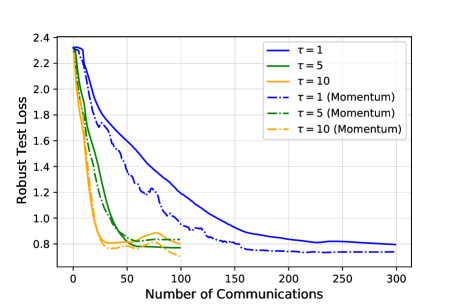
Figure 3: Robust test loss for the CIFAR10 experiment shown in Section 5.2. The test loss in Equation 9 is computed using some steps of gradient ascent to find an estimate of ${\mathbf{y}}^{*}$.

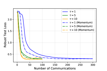
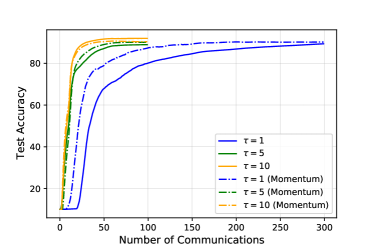
Figure 4: Comparison of the effects of $\tau$ on the performance of Local SGDA and Momentum Local SGDA algorithms, for the robust NN training problem on the FashionMNIST dataset, with the VGG11 model. The figures show the robust test loss and robust test accuracy.

References

• Arjevani et al. (2019) Arjevani, Y., Carmon, Y., Duchi, J. C., Foster, D. J., Srebro, N., and Woodworth, B. Lower bounds for non-convex stochastic optimization. arXiv preprint arXiv:1912.02365, 2019.
• Arjovsky et al. (2017) Arjovsky, M., Chintala, S., and Bottou, L. Wasserstein generative adversarial networks. In International conference on machine learning, pp. 214–223. PMLR, 2017.
• Beznosikov et al. (2020) Beznosikov, A., Samokhin, V., and Gasnikov, A. Distributed saddle-point problems: Lower bounds, optimal algorithms and federated gans. arXiv preprint arXiv:2010.13112, 2020.
• Beznosikov et al. (2021a) Beznosikov, A., Dvurechensky, P., Koloskova, A., Samokhin, V., Stich, S. U., and Gasnikov, A. Decentralized local stochastic extra-gradient for variational inequalities. arXiv preprint arXiv:2106.08315, 2021a.
• Beznosikov et al. (2021b) Beznosikov, A., Richtárik, P., Diskin, M., Ryabinin, M., and Gasnikov, A. Distributed methods with compressed communication for solving variational inequalities, with theoretical guarantees. arXiv preprint arXiv:2110.03313, 2021b.
• Beznosikov et al. (2021c) Beznosikov, A., Rogozin, A., Kovalev, D., and Gasnikov, A. Near-optimal decentralized algorithms for saddle point problems over time-varying networks. In International Conference on Optimization and Applications, pp.  246–257. Springer, 2021c.
• Beznosikov et al. (2021d) Beznosikov, A., Scutari, G., Rogozin, A., and Gasnikov, A. Distributed saddle-point problems under similarity. In Advances in Neural Information Processing Systems, volume 34, 2021d.
• Beznosikov et al. (2021e) Beznosikov, A., Sushko, V., Sadiev, A., and Gasnikov, A. Decentralized personalized federated min-max problems. arXiv preprint arXiv:2106.07289, 2021e.
• Bonawitz et al. (2019) Bonawitz, K., Eichner, H., Grieskamp, W., Huba, D., Ingerman, A., Ivanov, V., Kiddon, C., Konečnỳ, J., Mazzocchi, S., McMahan, H. B., et al. Towards federated learning at scale: System design. arXiv preprint arXiv:1902.01046, 2019.
• Bottou et al. (2018) Bottou, L., Curtis, F. E., and Nocedal, J. Optimization methods for large-scale machine learning. Siam Review, 60(2):223–311, 2018.
• Charles & Papailiopoulos (2018) Charles, Z. and Papailiopoulos, D. Stability and generalization of learning algorithms that converge to global optima. In International Conference on Machine Learning, pp. 745–754. PMLR, 2018.
• Chen et al. (2020a) Chen, X., Yang, S., Shen, L., and Pang, X. A distributed training algorithm of generative adversarial networks with quantized gradients. arXiv preprint arXiv:2010.13359, 2020a.
• Chen et al. (2020b) Chen, Z., Zhou, Y., Xu, T., and Liang, Y. Proximal gradient descent-ascent: Variable convergence under kł geometry. In International Conference on Learning Representations, 2020b.
• Dai et al. (2017) Dai, B., He, N., Pan, Y., Boots, B., and Song, L. Learning from conditional distributions via dual embeddings. In Artificial Intelligence and Statistics, pp.  1458–1467. PMLR, 2017.
• Dai et al. (2018) Dai, B., Shaw, A., Li, L., Xiao, L., He, N., Liu, Z., Chen, J., and Song, L. Sbeed: Convergent reinforcement learning with nonlinear function approximation. In International Conference on Machine Learning, pp. 1125–1134. PMLR, 2018.
• Daskalakis et al. (2018) Daskalakis, C., Ilyas, A., Syrgkanis, V., and Zeng, H. Training gans with optimism. In International Conference on Learning Representations (ICLR 2018), 2018.
• Daskalakis et al. (2021) Daskalakis, C., Skoulakis, S., and Zampetakis, M. The complexity of constrained min-max optimization. In Proceedings of the 53rd Annual ACM SIGACT Symposium on Theory of Computing, pp.  1466–1478, 2021.
• Davis & Drusvyatskiy (2019) Davis, D. and Drusvyatskiy, D. Stochastic model-based minimization of weakly convex functions. SIAM Journal on Optimization, 29(1):207–239, 2019.
• Deng & Mahdavi (2021) Deng, Y. and Mahdavi, M. Local stochastic gradient descent ascent: Convergence analysis and communication efficiency. In International Conference on Artificial Intelligence and Statistics, pp.  1387–1395. PMLR, 2021.
• Deng et al. (2020) Deng, Y., Kamani, M. M., and Mahdavi, M. Distributionally robust federated averaging. In Advances in Neural Information Processing Systems, volume 33, pp.  15111–15122, 2020.
• Diakonikolas et al. (2021) Diakonikolas, J., Daskalakis, C., and Jordan, M. Efficient methods for structured nonconvex-nonconcave min-max optimization. In International Conference on Artificial Intelligence and Statistics, pp.  2746–2754. PMLR, 2021.
• Drusvyatskiy & Paquette (2019) Drusvyatskiy, D. and Paquette, C. Efficiency of minimizing compositions of convex functions and smooth maps. Mathematical Programming, 178(1):503–558, 2019.
• Fiez et al. (2021) Fiez, T., Ratliff, L., Mazumdar, E., Faulkner, E., and Narang, A. Global convergence to local minmax equilibrium in classes of nonconvex zero-sum games. Advances in Neural Information Processing Systems, 34, 2021.
• Goodfellow et al. (2014) Goodfellow, I., Pouget-Abadie, J., Mirza, M., Xu, B., Warde-Farley, D., Ozair, S., Courville, A., and Bengio, Y. Generative adversarial nets. In Advances in neural information processing systems, volume 27, 2014.
• Gu et al. (2021) Gu, X., Huang, K., Zhang, J., and Huang, L. Fast federated learning in the presence of arbitrary device unavailability. In Advances in Neural Information Processing Systems, volume 34, 2021.
• Gulrajani et al. (2017) Gulrajani, I., Ahmed, F., Arjovsky, M., Dumoulin, V., and Courville, A. C. Improved training of wasserstein gans. In Advances in Neural Information Processing Systems, volume 30, 2017.
• Guminov & Gasnikov (2017) Guminov, S. and Gasnikov, A. Accelerated methods for $\alpha$-weakly-quasi-convex problems. arXiv preprint arXiv:1710.00797, 2017.
• Guo et al. (2020) Guo, Z., Liu, M., Yuan, Z., Shen, L., Liu, W., and Yang, T. Communication-efficient distributed stochastic AUC maximization with deep neural networks. In International Conference on Machine Learning, pp. 3864–3874. PMLR, 2020.
• Haddadpour & Mahdavi (2019) Haddadpour, F. and Mahdavi, M. On the convergence of local descent methods in federated learning. arXiv preprint arXiv:1910.14425, 2019.
• Heusel et al. (2017) Heusel, M., Ramsauer, H., Unterthiner, T., Nessler, B., and Hochreiter, S. Gans trained by a two time-scale update rule converge to a local nash equilibrium. Advances in neural information processing systems, 30, 2017.
• Hinder et al. (2020) Hinder, O., Sidford, A., and Sohoni, N. Near-optimal methods for minimizing star-convex functions and beyond. In Conference on Learning Theory, pp.  1894–1938. PMLR, 2020.
• Hou et al. (2021) Hou, C., Thekumparampil, K. K., Fanti, G., and Oh, S. Efficient algorithms for federated saddle point optimization. arXiv preprint arXiv:2102.06333, 2021.
• Hsieh et al. (2021) Hsieh, Y.-P., Mertikopoulos, P., and Cevher, V. The limits of min-max optimization algorithms: Convergence to spurious non-critical sets. In International Conference on Machine Learning, pp. 4337–4348. PMLR, 2021.
• Jacot et al. (2018) Jacot, A., Gabriel, F., and Hongler, C. Neural tangent kernel: convergence and generalization in neural networks. In Advances in Neural Information Processing Systems, volume 31, pp.  8580–8589, 2018.
• Jiang & Agrawal (2018) Jiang, P. and Agrawal, G. A linear speedup analysis of distributed deep learning with sparse and quantized communication. In Advances in Neural Information Processing Systems, pp. 2530–2541, 2018.
• Jin et al. (2020) Jin, C., Netrapalli, P., and Jordan, M. What is local optimality in nonconvex-nonconcave minimax optimization? In International Conference on Machine Learning, pp. 4880–4889. PMLR, 2020.
• Jin (2020) Jin, J. On the convergence of first order methods for quasar-convex optimization. arXiv preprint arXiv:2010.04937, 2020.
• Kairouz et al. (2019) Kairouz, P., McMahan, H. B., Avent, B., Bellet, A., Bennis, M., Bhagoji, A. N., Bonawitz, K., Charles, Z., Cormode, G., Cummings, R., et al. Advances and open problems in federated learning. arXiv preprint arXiv:1912.04977, 2019.
• Karimi et al. (2016) Karimi, H., Nutini, J., and Schmidt, M. Linear convergence of gradient and proximal-gradient methods under the polyak-łojasiewicz condition. In Joint European Conference on Machine Learning and Knowledge Discovery in Databases, pp.  795–811. Springer, 2016.
• Khaled et al. (2020) Khaled, A., Mishchenko, K., and Richtárik, P. Tighter theory for local sgd on identical and heterogeneous data. In International Conference on Artificial Intelligence and Statistics, pp.  4519–4529. PMLR, 2020.
• Kleinberg et al. (2018) Kleinberg, B., Li, Y., and Yuan, Y. An alternative view: When does sgd escape local minima? In International Conference on Machine Learning, pp. 2698–2707. PMLR, 2018.
• Koloskova et al. (2020) Koloskova, A., Loizou, N., Boreiri, S., Jaggi, M., and Stich, S. A unified theory of decentralized sgd with changing topology and local updates. In International Conference on Machine Learning, pp. 5381–5393. PMLR, 2020.
• Konečnỳ et al. (2016) Konečnỳ, J., McMahan, H. B., Ramage, D., and Richtárik, P. Federated optimization: Distributed machine learning for on-device intelligence. arXiv preprint arXiv:1610.02527, 2016.
• Léauté & Faltings (2013) Léauté, T. and Faltings, B. Protecting privacy through distributed computation in multi-agent decision making. Journal of Artificial Intelligence Research, 47:649–695, 2013.
• Lee & Kim (2021) Lee, S. and Kim, D. Fast extra gradient methods for smooth structured nonconvex-nonconcave minimax problems. In Advances in Neural Information Processing Systems, volume 34, 2021.
• Lei et al. (2021) Lei, Y., Yang, Z., Yang, T., and Ying, Y. Stability and generalization of stochastic gradient methods for minimax problems. In International Conference on Machine Learning, pp. 6175–6186. PMLR, 2021.
• Li et al. (2021) Li, H., Tian, Y., Zhang, J., and Jadbabaie, A. Complexity lower bounds for nonconvex-strongly-concave min-max optimization. In Advances in Neural Information Processing Systems, volume 34, 2021.
• Li & Yuan (2017) Li, Y. and Yuan, Y. Convergence analysis of two-layer neural networks with relu activation. In Advances in Neural Information Processing Systems, volume 30, 2017.
• Liao et al. (2021) Liao, L., Shen, L., Duan, J., Kolar, M., and Tao, D. Local adagrad-type algorithm for stochastic convex-concave minimax problems. arXiv preprint arXiv:2106.10022, 2021.
• Lin et al. (2020a) Lin, T., Jin, C., and Jordan, M. On gradient descent ascent for nonconvex-concave minimax problems. In International Conference on Machine Learning, pp. 6083–6093. PMLR, 2020a.
• Lin et al. (2020b) Lin, T., Jin, C., and Jordan, M. I. Near-optimal algorithms for minimax optimization. In Conference on Learning Theory, pp.  2738–2779. PMLR, 2020b.
• Liu et al. (2022) Liu, C., Zhu, L., and Belkin, M. Loss landscapes and optimization in over-parameterized non-linear systems and neural networks. Applied and Computational Harmonic Analysis, 2022.
• Liu et al. (2020) Liu, M. L., Mroueh, Y., Zhang, W., Cui, X., Ross, J., and Das, P. Decentralized parallel algorithm for training generative adversarial nets. In Advances in Neural Information Processing Systems, volume 33, pp.  11056–11070, 2020.
• Liu et al. (2019) Liu, W., Mokhtari, A., Ozdaglar, A., Pattathil, S., Shen, Z., and Zheng, N. A decentralized proximal point-type method for saddle point problems. arXiv preprint arXiv:1910.14380, 2019.
• Lu et al. (2020) Lu, S., Tsaknakis, I., Hong, M., and Chen, Y. Hybrid block successive approximation for one-sided non-convex min-max problems: algorithms and applications. IEEE Transactions on Signal Processing, 68:3676–3691, 2020.
• Luo et al. (2020) Luo, L., Ye, H., Huang, Z., and Zhang, T. Stochastic recursive gradient descent ascent for stochastic nonconvex-strongly-concave minimax problems. In Advances in Neural Information Processing Systems, volume 33, pp.  20566–20577, 2020.
• Luo et al. (2021) Luo, L., Xie, G., Zhang, T., and Zhang, Z. Near optimal stochastic algorithms for finite-sum unbalanced convex-concave minimax optimization. arXiv preprint arXiv:2106.01761, 2021.
• Madry et al. (2018) Madry, A., Makelov, A., Schmidt, L., Tsipras, D., and Vladu, A. Towards deep learning models resistant to adversarial attacks. In International Conference on Learning Representations, 2018.
• McMahan et al. (2017) McMahan, B., Moore, E., Ramage, D., Hampson, S., and y Arcas, B. A. Communication-efficient learning of deep networks from decentralized data. In Artificial Intelligence and Statistics, pp.  1273–1282. PMLR, 2017.
• Mertikopoulos et al. (2018) Mertikopoulos, P., Lecouat, B., Zenati, H., Foo, C.-S., Chandrasekhar, V., and Piliouras, G. Optimistic mirror descent in saddle-point problems: Going the extra (gradient) mile. In International Conference on Learning Representations, 2018.
• Mohri et al. (2019) Mohri, M., Sivek, G., and Suresh, A. T. Agnostic federated learning. In International Conference on Machine Learning, pp. 4615–4625. PMLR, 2019.
• Namkoong & Duchi (2016) Namkoong, H. and Duchi, J. C. Stochastic gradient methods for distributionally robust optimization with f-divergences. In Advances in Neural Information Processing Systems, volume 29, 2016.
• Namkoong & Duchi (2017) Namkoong, H. and Duchi, J. C. Variance-based regularization with convex objectives. In Advances in Neural Information Processing Systems, volume 30, 2017.
• Nedić & Ozdaglar (2009) Nedić, A. and Ozdaglar, A. Subgradient methods for saddle-point problems. Journal of optimization theory and applications, 142(1):205–228, 2009.
• Nemirovski (2004) Nemirovski, A. Prox-method with rate of convergence o (1/t) for variational inequalities with lipschitz continuous monotone operators and smooth convex-concave saddle point problems. SIAM Journal on Optimization, 15(1):229–251, 2004.
• Nesterov (2018) Nesterov, Y. Lectures on convex optimization, volume 137. Springer, 2018.
• Nouiehed et al. (2019) Nouiehed, M., Sanjabi, M., Huang, T., Lee, J. D., and Razaviyayn, M. Solving a class of non-convex min-max games using iterative first order methods. In Advances in Neural Information Processing Systems, volume 32, pp.  14934–14942, 2019.
• Ouyang & Xu (2021) Ouyang, Y. and Xu, Y. Lower complexity bounds of first-order methods for convex-concave bilinear saddle-point problems. Mathematical Programming, 185(1):1–35, 2021.
• Polyak (1963) Polyak, B. T. Gradient methods for minimizing functionals. Zhurnal vychislitel’noi matematiki i matematicheskoi fiziki, 3(4):643–653, 1963.
• Qiu et al. (2020) Qiu, S., Yang, Z., Wei, X., Ye, J., and Wang, Z. Single-timescale stochastic nonconvex-concave optimization for smooth nonlinear TD learning. arXiv preprint arXiv:2008.10103, 2020.
• Rafique et al. (2021) Rafique, H., Liu, M., Lin, Q., and Yang, T. Weakly-convex–concave min–max optimization: provable algorithms and applications in machine learning. Optimization Methods and Software, pp.  1–35, 2021.
• Reisizadeh et al. (2020) Reisizadeh, A., Farnia, F., Pedarsani, R., and Jadbabaie, A. Robust federated learning: The case of affine distribution shifts. In Advances in Neural Information Processing Systems, volume 33, pp.  21554–21565, 2020.
• Rogozin et al. (2021) Rogozin, A., Beznosikov, A., Dvinskikh, D., Kovalev, D., Dvurechensky, P., and Gasnikov, A. Decentralized distributed optimization for saddle point problems. arXiv preprint arXiv:2102.07758, 2021.
• Ruan et al. (2021) Ruan, Y., Zhang, X., Liang, S.-C., and Joe-Wong, C. Towards flexible device participation in federated learning. In International Conference on Artificial Intelligence and Statistics, pp.  3403–3411. PMLR, 2021.
• Shen et al. (2021) Shen, Y., Du, J., Zhao, H., Zhang, B., Ji, Z., and Gao, M. FedMM: Saddle point optimization for federated adversarial domain adaptation. arXiv preprint arXiv:2110.08477, 2021.
• Sinha et al. (2017) Sinha, A., Namkoong, H., and Duchi, J. Certifiable distributional robustness with principled adversarial training. In International Conference on Learning Representations, 2017.
• Spiridonoff et al. (2021) Spiridonoff, A., Olshevsky, A., and Paschalidis, I. C. Communication-efficient sgd: From local sgd to one-shot averaging. In Advances in Neural Information Processing Systems, volume 34, 2021.
• Stich (2018) Stich, S. U. Local sgd converges fast and communicates little. In International Conference on Learning Representations, 2018.
• Stich & Karimireddy (2020) Stich, S. U. and Karimireddy, S. P. The error-feedback framework: Better rates for sgd with delayed gradients and compressed updates. Journal of Machine Learning Research, 21:1–36, 2020.
• Thekumparampil et al. (2019) Thekumparampil, K. K., Jain, P., Netrapalli, P., and Oh, S. Efficient algorithms for smooth minimax optimization. In Advances in Neural Information Processing Systems, volume 32, 2019.
• Tran-Dinh et al. (2020) Tran-Dinh, Q., Liu, D., and Nguyen, L. M. Hybrid variance-reduced sgd algorithms for minimax problems with nonconvex-linear function. In Advances in Neural Information Processing Systems, volume 33, pp.  11096–11107, 2020.
• Wang et al. (2019) Wang, H., Yurochkin, M., Sun, Y., Papailiopoulos, D., and Khazaeni, Y. Federated learning with matched averaging. In International Conference on Learning Representations, 2019.
• Wang & Joshi (2021) Wang, J. and Joshi, G. Cooperative SGD: A unified framework for the design and analysis of local-update sgd algorithms. Journal of Machine Learning Research, 22(213):1–50, 2021.
• Wang et al. (2020) Wang, J., Liu, Q., Liang, H., Joshi, G., and Poor, H. V. Tackling the objective inconsistency problem in heterogeneous federated optimization. In Advances in Neural Information Processing Systems, volume 33, pp.  7611–7623, 2020.
• Wang et al. (2021) Wang, J., Zhang, T., Liu, S., Chen, P.-Y., Xu, J., Fardad, M., and Li, B. Adversarial attack generation empowered by min-max optimization. Advances in Neural Information Processing Systems, 34, 2021.
• Wang & Li (2020) Wang, Y. and Li, J. Improved algorithms for convex-concave minimax optimization. In Advances in Neural Information Processing Systems, volume 33, pp.  4800–4810, 2020.
• Xian et al. (2021) Xian, W., Huang, F., Zhang, Y., and Huang, H. A faster decentralized algorithm for nonconvex minimax problems. In Advances in Neural Information Processing Systems, volume 34, 2021.
• Xiao et al. (2017) Xiao, H., Rasul, K., and Vollgraf, R. Fashion-mnist: a novel image dataset for benchmarking machine learning algorithms. arXiv preprint arXiv:1708.07747, 2017.
• Xie et al. (2020) Xie, G., Luo, L., Lian, Y., and Zhang, Z. Lower complexity bounds for finite-sum convex-concave minimax optimization problems. In International Conference on Machine Learning, pp. 10504–10513. PMLR, 2020.
• Xie et al. (2021) Xie, J., Zhang, C., Zhang, Y., Shen, Z., and Qian, H. A federated learning framework for nonconvex-pl minimax problems. arXiv preprint arXiv:2105.14216, 2021.
• Xing et al. (2016) Xing, E. P., Ho, Q., Xie, P., and Wei, D. Strategies and principles of distributed machine learning on big data. Engineering, 2(2):179–195, 2016.
• Xu et al. (2020) Xu, Z., Zhang, H., Xu, Y., and Lan, G. A unified single-loop alternating gradient projection algorithm for nonconvex-concave and convex-nonconcave minimax problems. arXiv preprint arXiv:2006.02032, 2020.
• Yang et al. (2021a) Yang, H., Fang, M., and Liu, J. Achieving linear speedup with partial worker participation in non-iid federated learning. In International Conference on Learning Representations, 2021a.
• Yang et al. (2020a) Yang, J., Kiyavash, N., and He, N. Global convergence and variance reduction for a class of nonconvex-nonconcave minimax problems. In Advances in Neural Information Processing Systems, volume 33, pp.  1153–1165, 2020a.
• Yang et al. (2020b) Yang, J., Zhang, S., Kiyavash, N., and He, N. A catalyst framework for minimax optimization. In Advances in Neural Information Processing Systems, volume 33, pp.  5667–5678, 2020b.
• Yang et al. (2021b) Yang, J., Orvieto, A., Lucchi, A., and He, N. Faster single-loop algorithms for minimax optimization without strong concavity. arXiv preprint arXiv:2112.05604, 2021b.
• Yang et al. (2018) Yang, T., Andrew, G., Eichner, H., Sun, H., Li, W., Kong, N., Ramage, D., and Beaufays, F. Applied federated learning: Improving google keyboard query suggestions. arXiv preprint arXiv:1812.02903, 2018.
• Yoon & Ryu (2021) Yoon, T. and Ryu, E. K. Accelerated algorithms for smooth convex-concave minimax problems with o (1/k^2) rate on squared gradient norm. In International Conference on Machine Learning, pp. 12098–12109. PMLR, 2021.
• Yu et al. (2019) Yu, H., Jin, R., and Yang, S. On the linear speedup analysis of communication efficient momentum SGD for distributed non-convex optimization. In International Conference on Machine Learning, pp. 7184–7193. PMLR, 2019.
• Yuan et al. (2021) Yuan, Z., Guo, Z., Xu, Y., Ying, Y., and Yang, T. Federated deep AUC maximization for heterogeneous data with a constant communication complexity. In International Conference on Machine Learning, pp. 12219–12229. PMLR, 2021.
• Zhang et al. (2020) Zhang, J., Xiao, P., Sun, R., and Luo, Z. A single-loop smoothed gradient descent-ascent algorithm for nonconvex-concave min-max problems. In Advances in Neural Information Processing Systems, volume 33, pp.  7377–7389, 2020.
• Zhang et al. (2021) Zhang, S., Yang, J., Guzmán, C., Kiyavash, N., and He, N. The complexity of nonconvex-strongly-concave minimax optimization. In Conference on Uncertainty in Artificial Intelligence, pp. 482–492. PMLR, 2021.
• Zhou & Cong (2018) Zhou, F. and Cong, G. On the convergence properties of a k-step averaging stochastic gradient descent algorithm for nonconvex optimization. In Proceedings of the 27th International Joint Conference on Artificial Intelligence, pp.  3219–3227, 2018.