Coarse-to-Fine Sparse Transformer for Hyperspectral Image Reconstruction

Abstract

Many algorithms have been developed to solve the inverse problem of coded aperture snapshot spectral imaging (CASSI), $i.e.$, recovering the 3D hyperspectral images (HSIs) from a 2D compressive measurement. In recent years, learning-based methods have demonstrated promising performance and dominated the mainstream research direction. However, existing CNN-based methods show limitations in capturing long-range dependencies and non-local self-similarity. Previous Transformer-based methods densely sample tokens, some of which are uninformative, and calculate the multi-head self-attention (MSA) between some tokens that are unrelated in content. This does not fit the spatially sparse nature of HSI signals and limits the model scalability. In this paper, we propose a novel Transformer-based method, coarse-to-fine sparse Transformer (CST), firstly embedding HSI sparsity into deep learning for HSI reconstruction. In particular, CST uses our proposed spectra-aware screening mechanism (SASM) for $coarse~{}patch$ $selecting$. Then the selected patches are fed into our customized spectra-aggregation hashing multi-head self-attention (SAH-MSA) for $fine~{}pixel$ $clustering$ and self-similarity capturing. Comprehensive experiments show that our CST significantly outperforms state-of-the-art methods while requiring cheaper computational costs. https://github.com/caiyuanhao1998/MST

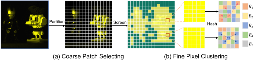
Figure 1: Diagram of our coarse-to-fine learning scheme. (a) HSIs exhibit high spatial sparsity. The image is firstly partitioned into non-overlapping patches. Then the informative patches (yellow) with HSI signals are screened out and fed into the self-attention mechanism. (b) Tokens closely correlated in content are clustered into the same $bucket$ ($B_{1}\sim B_{5}$). Then the self-attention is calculated inside each $bucket$.

1 Introduction

Hyperspectral images (HSIs), which contain multiple continuous and narrow spectral bands, can provide more detailed information of the captured scene than normal RGB images. Based on the inherently rich and detailed spectral signatures, HSIs have been widely applied to many computer vision tasks and graphical applications, $e.g.,$ image classification [26, 58, 102], object tracking [30, 40, 76, 77], remote sensing [4, 62, 74, 96], medical imaging [1, 54, 65], $etc$.

To collect HSI cubes, traditional imaging systems scan the scenes with multiple exposures using 1D or 2D sensors. This imaging process is time-consuming and limited to static objects [38]. Thus, conventional imaging systems cannot capture dynamic scenes. Recently, researchers have developed several snapshot compressive imaging (SCI) systems to capture HSIs, where the 3D HSI cube is compressed into a single 2D measurement [10, 11, 59, 79]. Among these SCI systems, coded aperture snapshot spectral imaging (CASSI) stands out as a promising solution and has become an active research direction [31, 37, 64, 79]. CASSI systems modulate HSI signals at different wavelengths by a coded aperture (physical mask) and then vary the modulation by a disperser, i.e., to shift the modulated images at different wavelengths to different spatial locations on the detector plane. Subsequently, a reconstruction algorithm is used to restore the 3D HSI cube from the 2D compressive image, which is a core task in CASSI.

To solve this ill-posed inverse problem, traditional methods [51, 83, 94] mainly depend on hand-crafted priors and assumptions. The main drawbacks of these model-based methods are that they need to tweak parameters manually, leading to poor generality and slow reconstruction speed. In recent years, deep learning methods have shown the potential to speed up the reconstruction and improve restoration quality for natural images [5, 34, 35, 36, 71, 98, 99, 100, 101, 103, 104]. Hence, convolution neural networks (CNNs) have been used to learn the underlying mapping function from the 2D compressive measurement to the 3D HSI signal. Nevertheless, these CNN-based methods yield impressive results but show limitations in capturing non-local self-similarity and long-range dependencies.

In the past few years, the natural language processing (NLP) model Transformer [78] has gained much popularity and achieved great success in computer vision. Transformer provides a powerful model that excels at exploring global inter-dependence between different regions to alleviate the constraints of CNN-based methods. Nonetheless, directly applying vision Transformers to HSI reconstruction encounters two main issues that cannot be ignored. Firstly, the HSI signals exhibit high spatial sparsity as shown in Fig. 1 (a). Some dark regions are almost uninformative. However, previous local [52] or global [22] Transformers process all spatial pixel vectors inside non-overlapping windows or global images into tokens without screening and then feed the tokens into the multi-head self-attention (MSA) mechanism. Many regions with limited information are sampled, which dramatically degrades the model efficiency and limits the reconstruction performance. Secondly, previous Transformers linearly project all the tokens into $query$, $key$, and $value$, and then perform matrix multiplication for calculating MSA without clustering. Yet, some of the tokens are not related in content. Attending to all these tokens at once lowers down the cost-effectiveness of model and may easily lead to over-smooth results [45]. Besides, the computational complexity of global Transformer [22] is quadratic to the spatial dimensions, which is nontrivial and sometimes unaffordable. MST [6] calculates MSA along the spectral dimension, thus circumventing the HSI spatial sparsity.

Hence, how to combine HSI sparsity with learning-based algorithms still remains under-explored. This work aims to investigate this problem and cope with the limitations of existing CNN-based and Transformer-based methods.

In this paper, we propose a novel method, coarse-to-fine sparse Transformer (CST), for HSI reconstruction. Our CST composes two key techniques. Firstly, due to the large variation in HSI informativeness of spatial regions, we propose a spectra-aware screening mechanism (SASM) for coarse patch selecting. To be specific, in Fig. 1 (a), our SASM partitions the image into non-overlapping patches and then detects the patches that are informative of HSI representations. Subsequently, only the detected patches (yellow) are fed into the self-attention mechanisms to decrease the inefficient calculation of uninformative regions (green) and promote the model cost-effectiveness. Secondly, instead of using all projected tokens at once like previous Transformers, we aim to calculate self-attention of tokens that are closely related in content. Toward this end, we customize spectra-aggregation hashing multi-head self-attention (SAH-MSA) for fine pixel clustering as shown in Fig. 1 (b). SAH-MSA learns to cluster tokens into different groups (termed $buckets$ in this paper) by searching similar elements that produce the max inner product. Tokens inside each $bucket$ are considered closely related in content. Then the MSA operation is applied within each $bucket$. Finally, with the proposed techniques, we enable a coarse-to-fine learning scheme that embeds the HSI spatial sparsity into learning-based methods. We establish a series of small-to-large CST families that outperform state-of-the-art (SOTA) methods while requiring much cheaper computational costs.

The main contributions of this work can be summarized as follows:

• We propose a novel Transformer-based method, CST, for HSI reconstruction. To the best of our knowledge, it is the first attempt to embed the HSI spatial sparsity nature into learning-based algorithms for this task.

• We present SASM to locate informative regions with HSI signals.

• We customize SAH-MSA to capture interactions of closely related patterns.

• Our CST with much lower computational complexity significantly surpasses SOTA algorithms on all scenes in simulation. Moreover, our CST yields more visually pleasant results than existing methods in real HSI restoration.

2 Related Work

2.1 Hyperspectral Image Reconstruction

Conventional HSI reconstruction methods [3, 27, 50, 51, 83, 94] rely on hand-crafted image priors. For instance, gradient projection [27] algorithms are exploited to handle the HSI sparseness. In addition, total variation regularizers are employed by GAP-TV [94] while the low-rank property and non-local self-similarity are used in DeSCI [50]. Nonetheless, these traditional model-based methods suffer from low reconstruction speed and poor generalization ability. Recently, CNNs have been used to solve the inverse problem of spectral SCI. These CNN-based algorithms can be divided into three categories, i.e., end-to-end (E2E) methods, deep unfolding methods, and plug-and-play (PnP) methods. E2E algorithms [6, 29, 33, 64, 67, 89] apply a deep CNN as a powerful model to learn the E2E mapping function of HSI restoration. Deep unfolding methods [7, 28, 37, 57, 63, 82] employ multi-stage CNNs trained to map the measurements into the desired signal. Each stage contains two parts, i.e., linear projection and passing the signal through a CNN functioning as a denoiser. PnP methods [13, 72, 95] plug pre-trained CNN denoisers into model-based methods to solve the HSI reconstruction problem. Nonetheless, these CNN-based algorithms show limitations in capturing long-range spatial dependencies and modeling the non-local self-similarity. Besides, the sparsity property of HSI representations is not well addressed, posing a low-efficiency problem to HSI reconstruction models.

2.2 Vision Transformer

Transformer [78] is proposed for machine translation in NLP. Recently, it has gained much popularity in computer vision because of its superiority in modeling long-range interactions between spatial regions. Vision Transformer has been widely applied in image classification [2, 14, 22, 23, 32, 43, 73, 86, 87], object detection [12, 19, 20, 25, 68, 69, 93, 108], semantic segmentation [17, 52, 55, 75, 88, 92, 97, 107], human pose estimation [8, 39, 44, 46, 49, 56, 60, 106], and so on. Besides high-level vision, Transformer has also been used in image restoration [6, 9, 15, 21, 47, 48, 80, 84]. For example, Cai et al. [6] propose the first Transformer-based model MST for HSI reconstruction. MST treats spectral maps as tokens and calculates the self-attention along the spectral dimension. In addition, Wang et al. [84] propose a U-shaped Transformer, named UFormer, built by the basic blocks of Swin Transformer [52] for natural image restoration. However, existing Transformers densely sample tokens, some of which corresponding to the regions with limited information, and calculate MSA between some tokens that are unrelated in content. How to embed HSI spatial sparsity into Transformer to boost the model efficiency still remains under-studied. Our work aims to fill this research gap.

3 Mathematical Model of CASSI

Figure 2: A schematic diagram of CASSI.

A schematic diagram of CASSI is shown in Fig. 2. We denote the input 3D HSI data cube as $\mathbf{F}\in\mathbb{R}^{H\times W\times N_{\lambda}}$, where $H$, $W$, and $N_{\lambda}$ refer to the HSI’s height, width, and number of wavelengths, respectively. Firstly, a coded aperture ($i.e.$, a physical mask) $\mathbf{M^{*}}\in\mathbb{R}^{H\times W}$ is used to modulate $\mathbf{F}$ along the channel dimension:

$$\mathbf{F}^{\prime}(:,:,n_{\lambda})=\mathbf{F}(:,:,n_{\lambda})\odot\mathbf{M^{*}},\vspace{-1.2mm}$$ (1)

where $\mathbf{F}^{\prime}\in\mathbb{R}^{H\times W\times N_{\lambda}}$ indicates the modulated signals, $n_{\lambda}\in[1,\dots,N_{\lambda}]$ indexes the spectral wavelengths, and $\odot$ represents the element-wise product. After undergoing the disperser, $\mathbf{F}^{\prime}$ becomes tilted and could be treated as sheared along the $y$-axis. We denote this tilted data cube as $\mathbf{F}^{\prime\prime}\in\mathbb{R}^{H\times(W+d(N_{\lambda}-1))\times N_{\lambda}}$, where $d$ refers to the step of spatial shifting. Suppose $\lambda_{c}$ is the reference wavelength, which means that $\mathbf{F}^{\prime\prime}(:,:,n_{\lambda_{c}})$ works like an anchor image that is not sheared along the $y$-axis. Then the dispersion can be formulated as

$$\mathbf{F}^{\prime\prime}(u,v,n_{\lambda})=\mathbf{F}^{\prime}(x,y+d(\lambda_{n}-\lambda_{c}),n_{\lambda}),\vspace{-1.5mm}$$ (2)

where $(u,v)$ locates the coordinate on the sensoring detector, $\lambda_{n}$ represents the wavelength of the $n_{\lambda}$-th channel, and $d(\lambda_{n}-\lambda_{c})$ refers to the spatial shifting offset of the $n_{\lambda}$-th channel on $\mathbf{F}^{\prime\prime}$. Eventually, the data cube is compressed into a 2D measurement $\mathbf{Y}\in\mathbb{R}^{H\times(W+d(N_{\lambda}-1))}$ by integrating all the channels as

$$\mathbf{Y}=\sum_{n_{\lambda}=1}^{N_{\lambda}}\mathbf{F}^{\prime\prime}(:,:,n_{\lambda})+\mathbf{G},\vspace{-2mm}$$ (3)

where $\mathbf{G}\in\mathbb{R}^{H\times(W+d(N_{\lambda}-1))}$ is the random noise generated during the imaging process. Given the 2D measurement $\mathbf{Y}$ captured by CASSI, the core task of HSI reconstruction is to restore the 3D HSI data cube $\mathbf{F}$ as mentioned in Eq. (1).

4 Method

The overall framework of our coarse-to-fine sparse Transformer (CST) is shown in Fig. 3. CST consists of two key components, i.e., spectra-aware screening mechanism (SASM) for coarse patch selecting and spectra-aggregation hashing multi-head self-attention (SAH-MSA) for fine pixel clustering. Fig. 3 (a) depicts SASM and the network architecture of CST. Fig. 3 (b) shows the basic unit of CST, spectra-aware hashing attention block (SAHAB). Fig. 3 (c) illustrates our SAH-MSA, which is the most important component of SAHAB.

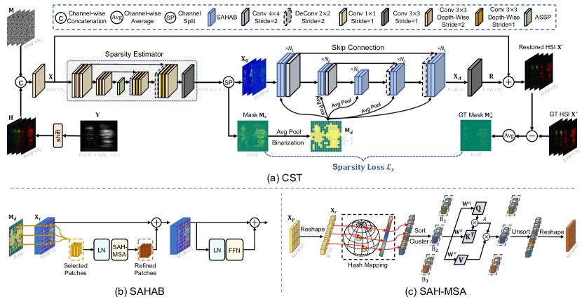
Figure 3: Framework of our method. (a) Spectra-aware screening mechanism (SASM) and the network architecture of CST. (b) The components of spectra-aware hashing attention block (SAHAB), which is the basic unit of CST. (c) spectra-aggregation hashing multi-head self-attention (SAH-MSA) is the key component embedding in SAHAB.

4.1 Network Architecture

Given a 2D measurement $\mathbf{Y}\in\mathbb{R}^{H\times(W+d(N_{\lambda}-1))}$, we reverse the dispersion in Eq. (2) and shift back $\mathbf{Y}$ to obtain an initialized input signal $\mathbf{H}\in\mathbb{R}^{H\times W\times N_{\lambda}}$ as

$$\mathbf{H}(x,y,n_{\lambda})=\mathbf{Y}(x,y-d(\lambda_{n}-\lambda_{c})).\vspace{-0.3mm}$$

Then $\mathbf{H}$ concatenated with the 3D physical mask $\mathbf{M}\in\mathbb{R}^{H\times W\times N_{\lambda}}$ (copy the physical mask $\mathbf{M^{*}}$ $N_{\lambda}$ times) passes through a $conv$1$\times$1 (convolutional layer with kernel size = 1$\times$1) to generate the initialized feature $\mathbf{X}\in\mathbb{R}^{H\times W\times N_{\lambda}}$.

Firstly, a sparsity estimator is developed to process $\mathbf{X}$ into a sparsity mask $\mathbf{M}_{s}\in\mathbb{R}^{H\times W}$ and shallow feature $\mathbf{X}_{0}\in\mathbb{R}^{H\times W\times C}$. The sparsity estimator is detailed in Sec. 4.2. Secondly, the shallow feature $\mathbf{X}_{0}$ passes through a three-stage symmetric encoder-decoder and is embedded into deep feature $\mathbf{X}_{d}\in\mathbb{R}^{H\times W\times C}$. The $i$-th stage of encoder or decoder contains $N_{i}$ SAHABs. As shown in Fig. 3 (b), SAHAB consists of two layer normalization (LN), an SAH-MSA, and a Feed-Forward Network (FFN). For feature downsampling and upsampling, we adopt strided $conv4\times 4$ and $deconv2\times 2$ layers, respectively. To alleviate the information loss caused by the downsample operation, the encoder features are aggregated with the decoder features via the identity connection. Finally, a $conv3\times 3$ is applied to $\mathbf{X}_{d}$ to produce the residual HSIs $\mathbf{R}\in\mathbb{R}^{H\times W\times N_{\lambda}}$. Then the reconstructed HSIs $\mathbf{X^{\prime}}$ can be obtained by the sum of $\mathbf{R}$ and $\mathbf{X}$ , $i.e.$, $\mathbf{X^{\prime}}=\mathbf{X}+\mathbf{R}$.

In our implementation, we set the basic channel $C$ = $N_{\lambda}$ = 28 to store the HSI information and change the combination ($N_{1}$,$N_{2}$,$N_{3}$) in Fig. 3 (a) to establish our CST families with small, medium, and large model sizes and computational complexities. They are CST-S (1,1,2), CST-M (2,2,2), and CST-L (2,4,6).

4.2 Spectra-Aware Screening Mechanism

We observe that the HSI signal exhibits high sparsity in the spatial dimension. However, the original global Transformer [22] samples all tokens on the feature map while the window-based local Transformer [52] samples all tokens inside every non-overlapping window. These Transformers sample many uninformative regions to calculate MSA, which degrades the model efficiency. To cope with this problem, we propose SASM for coarse patch selecting, i.e., screening out regions with dense HSI information to produce tokens. In this section, we introduce SASM in three parts, i.e., sparsity estimator, sparsity loss, and patch selection.

4.2.1 Sparsity Estimator.

In this part, we detail the sparsity estimator mentioned in Sec. 4. As shown in Fig. 3 (a), the sparsity estimator adopts a U-shaped structure including a two-stage encoder, an ASSP module [16], and a two-stage decoder. Each stage of the encoder consists of two $conv$1$\times$1 and a strided depth-wise $conv$3$\times$3. Each stage of the decoder contains a strided $deconv$2$\times$2, two $conv$1$\times$1, and a depth-wise $conv$3$\times$3. The sparsity estimator takes the initialized feature $\mathbf{X}$ as the input to produce the shallow feature $\mathbf{X}_{0}$ and the sparsity mask $\mathbf{M}_{s}$ that localizes and screens out the informative spatial regions with HSI representations. We achieve this by minimizing our proposed sparsity loss.

4.2.2 Sparsity Loss.

To supervise $\mathbf{M}_{s}$, we need a reference that can tell where the spatially sparse HSI information on the HSI is. Since the background is dark and uninformative, the regions with HSI representations are roughly equivalent to the regions that are hard to reconstruct. This statement can be verified by the visual analysis of sparsity mask in Sec. 5.4. Therefore, we design our reference signal $\mathbf{M}^{*}_{s}\in\mathbb{R}^{H\times W}$ by averaging the differences between the reconstructed HSIs $\mathbf{X}^{\prime}$ and the ground-truth HSIs $\mathbf{X}^{*}$ along the spectral dimension to avoid bias as

$$\mathbf{M}^{*}_{s}=\frac{1}{N_{\lambda}}\sum_{n_{\lambda}=1}^{N_{\lambda}}|\mathbf{X^{\prime}}(:,:,n_{\lambda})-\mathbf{X}^{*}(:,:,n_{\lambda})|.\vspace{-1mm}$$ (4)

Subsequently, our sparsity loss $\mathcal{L}_{s}$ is constructed as the mean squared error between the predicted sparsity mask $\mathbf{M}_{s}$ and the reference sparsity mask $\mathbf{M}^{*}_{s}$ as

$$\mathcal{L}_{s}=||\mathbf{M}_{s}-\mathbf{M}^{*}_{s}||_{2}.$$ (5)

By minimizing $\mathcal{L}_{s}$, the sparsity estimator is encouraged to detect the foreground hard-to-reconstruct regions with HSI representations. In addition, the overall training objective $\mathcal{L}$ is the weighted sum of $\mathcal{L}_{s}$ and $\mathcal{L}_{2}$ loss as

$$\mathcal{L}=\mathcal{L}_{2}+\lambda\cdot\mathcal{L}_{s}=||\mathbf{X}^{\prime}-\mathbf{X}^{*}||_{2}+\lambda\cdot||\mathbf{M}_{s}-\mathbf{M}^{*}_{s}||_{2},$$ (6)

where $\mathbf{X}^{*}$ represents the ground-truth HSIs and $\lambda$ refers to the hyperparameter that controls the importance balance between $\mathcal{L}_{2}$ and $\mathcal{L}_{s}$.

4.2.3 Patch Selection.

Our SASM partitions the feature map into non-overlapping patches at the size of $M\times M$. Then the patches with HSI representations are screened out by the predicted sparsity mask $\mathbf{M}_{s}$ and fed into SAH-MSA as shown in Fig. 3 (b). To be specific, $\mathbf{M}_{s}$ is firstly downsampled by average pooling and then binarized into $\mathbf{M}_{d}\in\mathbb{R}^{\frac{H}{M}\times\frac{W}{M}}$. We use a hyperparameter, sparsity ratio $\sigma$, to control the binarization. More specifically, we select the top $k$ patches with the highest values on the downsampled sparsity mask. $k$ is controlled by $\sigma$ that $k=\lfloor(1-\sigma)\frac{HW}{M^{2}}\rfloor$. Each pixel on $\mathbf{M}_{d}$ corresponds to an $M\times M$ patch on the feature map and its 0-1 value classifies whether this patch is screened out. Then $\mathbf{M}_{d}$ is applied to the SAH-MSA of each SAHAB. When $\mathbf{M}_{d}$ is used in the $i$-th stage ($i~{}>$ 1), an average pooling operation is exploited to downsample $\mathbf{M}_{d}$ into $\frac{1}{2^{i-1}}$ size to match the spatial resolution of the feature map of the $i$-th stage.

4.3 Spectra-Aggregation Hashing Multi-head Self-Attention.

Previous Transformers calculate MSA between all the sampled tokens, some of which are even unrelated in content. This may lead to inefficient computation that lowers down the model cost-effectiveness and easily hamper convergence [108]. The sparse coding methods [24, 61, 90, 91, 105] assume that image signals can be represented by a sparse linear combination over dictionary signals. Inspired by this, we propose SAH-MSA for $fine~{}pixel~{}clustering$. SAH-MSA enforces a sparsity constraint on the MSA mechanism. In particular, SAH-MSA only calculates self-attention between tokens that are closely correlated in content, which addresses the limitation of previous Transformers.

Our SAH-MSA learns to cluster tokens into different $buckets$ by searching elements that produce the max inner product. As shown in Fig. 3 (c), We denote a patch feature map as $\mathbf{X}_{p}\in\mathbb{R}^{M\times M\times C}$ that is screened out by the sparsity mask. We reshape $\mathbf{X}_{p}$ into $\mathbf{X}_{r}\in\mathbb{R}^{N\times C}$, where $N=M\times M$ is the number of elements. Subsequently, we use a hash function to aggregate the information in spectral wise and map a $C$-dimensional element (pixel vector) $\bm{x}\in\mathbb{R}^{C}$ into an integer hash code. We formulate this hash mapping $h:\mathbb{R}^{C}\to\mathbb{Z}$ as

$$h(\bm{x})=\lfloor\frac{\bm{a}\cdot\bm{x}+b}{r}\rfloor,$$ (7)

where $r\in\mathbb{R}$ is a constant, $\bm{a}\in\mathbb{R}^{C}$ and $b\in\mathbb{R}$ are random variables satisfying $\bm{a}=(a_{1},a_{2},...,a_{C})$ with $a_{i}\sim\mathcal{N}(0,1)$ and $b\sim\mathcal{U}(0,r)$ follows a uniform distribution. Then we sort the elements in $\mathbf{X}_{r}$ according to their hash codes. The $i$-th sorted element is denoted as $\bm{x}_{i}\in\mathbb{R}^{C}$. Then we split the elements into $buckets$ as

$$\mathbf{B}_{i}=\{\bm{x}_{j}:im+1\leq j\leq(i+1)m\},$$ (8)

where $\mathbf{B}_{i}$ represents the $i$-th $bucket$. Each $bucket$ has $m$ elements. There are $\frac{M\times M}{m}$ $buckets$ in total. With our hash clustering scheme, the closely content-correlated tokens are grouped into the same $bucket$. Therefore, the model can reduce the computational burden between content-unrelated elements by only applying the MSA operation to the tokens within the same $bucket$. More specifically, for a $query$ element $\bm{q}\in\mathbf{B}_{i}$, our SAH-MSA can be formulated as

$$\text{SAH-MSA}(\bm{q},\mathbf{B}_{i})=\sum_{n=1}^{N}\mathbf{W}_{n}~{}\text{head}_{n}(\bm{q},\mathbf{B}_{i}),$$ (9)

where $N$ is the number of attention heads. $\mathbf{W}_{n}\in\mathbb{R}^{C\times d}$ and $\mathbf{W^{\prime}}_{n}\in\mathbb{R}^{d\times C}$ are learnable parameters, where $d=\frac{C}{N}$ denotes the dimension of each head. ${A}_{n\bm{q}\bm{k}}$ and $\text{head}_{n}$ refer to the attention and output of the $n$-th head, formulated as

$$\mathbf{A}_{n\bm{q}\bm{k}}=\underset{\bm{k}\in\mathbf{B}_{i}}{\text{softmax}}(\frac{\bm{q}^{T}\mathbf{U}_{n}^{T}\mathbf{V}_{n}\bm{k}}{\sqrt{d}}),~{}~{}~{}~{}\text{head}_{n}(\bm{q},\mathbf{B}_{i})=\sum_{\bm{k}\in\mathbf{B}_{i}}\mathbf{A}_{n\bm{q}\bm{k}}\mathbf{W^{\prime}}_{n}\bm{k},$$ (10)

where $\mathbf{U}_{n}$ and $\mathbf{V}_{n}\in\mathbb{R}^{d\times C}$ are learnable parameters. With our hashing scheme, the similar elements are at small possibility to fall into different $buckets$. This probability can be further reduced by conducting multiple rounds of hashing in parallel [42]. $\mathbf{B}_{i}^{r}$ denotes the $i$-th $bucket$ of the $r$-th round. Then for each head, the multi-round output is the weighted sum of each single-round output, i.e.,

$$\text{head}_{n}(\bm{q},\mathbf{B}_{i})=\sum_{r=1}^{R}w^{r}_{n}~{}\text{head}_{n}(\bm{q},\mathbf{B}_{i}^{r}),$$ (11)

where $R$ refers to the round number and $w^{r}_{n}$ represents the weight importance of the $r$-th round in the $n$-th head, which scores the similarity between the $query$ element $\bm{q}$ and the elements belonging to $bucket$ $\mathbf{B}_{i}^{r}$. $w^{r}_{n}$ can be obtained by

$$w^{r}_{n}=\frac{\sum_{\bm{k}\in\mathbf{B}_{i}^{r}}A_{n\bm{q}\bm{k}}}{\sum_{\hat{r}=1}^{R}\sum_{\bm{k}\in\mathbf{B}_{i}^{\hat{r}}}A_{n\bm{q}\bm{k}}}.$$ (12)

Table 1: Comparisons of Params, FLOPS, PSNR (upper entry in each cell), and SSIM (lower entry in each cell) of different methods on 10 simulation scenes (S1$\sim$S10). Best results are in bold. * denotes setting the sparsity ratio to 0.

Algorithms	Params	GFLOPS	S1	S2	S3	S4	S5	S6	S7	S8	S9	S10	Avg
TwIST [3]	-	-	25.16 0.700	23.02 0.604	21.40 0.711	30.19 0.851	21.41 0.635	20.95 0.644	22.20 0.643	21.82 0.650	22.42 0.690	22.67 0.569	23.12 0.669
GAP-TV [94]	-	-	26.82 0.754	22.89 0.610	26.31 0.802	30.65 0.852	23.64 0.703	21.85 0.663	23.76 0.688	21.98 0.655	22.63 0.682	23.10 0.584	24.36 0.669
DeSCI [50]	-	-	27.13 0.748	23.04 0.620	26.62 0.818	34.96 0.897	23.94 0.706	22.38 0.683	24.45 0.743	22.03 0.673	24.56 0.732	23.59 0.587	25.27 0.721
$\lambda$-net [67]	62.64M	117.98	30.10 0.849	28.49 0.805	27.73 0.870	37.01 0.934	26.19 0.817	28.64 0.853	26.47 0.806	26.09 0.831	27.50 0.826	27.13 0.816	28.53 0.841
HSSP [81]	-	-	31.48 0.858	31.09 0.842	28.96 0.823	34.56 0.902	28.53 0.808	30.83 0.877	28.71 0.824	30.09 0.881	30.43 0.868	28.78 0.842	30.35 0.852
DNU [82]	1.19M	163.48	31.72 0.863	31.13 0.846	29.99 0.845	35.34 0.908	29.03 0.833	30.87 0.887	28.99 0.839	30.13 0.885	31.03 0.876	29.14 0.849	30.74 0.863
DIP-HSI [66]	33.85M	64.42	32.68 0.890	27.26 0.833	31.30 0.914	40.54 0.962	29.79 0.900	30.39 0.877	28.18 0.913	29.44 0.874	34.51 0.927	28.51 0.851	31.26 0.894
TSA-Net [64]	44.25M	110.06	32.03 0.892	31.00 0.858	32.25 0.915	39.19 0.953	29.39 0.884	31.44 0.908	30.32 0.878	29.35 0.888	30.01 0.890	29.59 0.874	31.46 0.894
DGSMP [37]	3.76M	646.65	33.26 0.915	32.09 0.898	33.06 0.925	40.54 0.964	28.86 0.882	33.08 0.937	30.74 0.886	31.55 0.923	31.66 0.911	31.44 0.925	32.63 0.917
HDNet [33]	2.37M	154.76	35.14 0.935	35.67 0.940	36.03 0.943	42.30 0.969	32.69 0.946	34.46 0.952	33.67 0.926	32.48 0.941	34.89 0.942	32.38 0.937	34.97 0.943
MST-S [6]	0.93M	12.96	34.71 0.930	34.45 0.925	35.32 0.943	41.50 0.967	31.90 0.933	33.85 0.943	32.69 0.911	31.69 0.933	34.67 0.939	31.82 0.926	34.26 0.935
MST-M [6]	1.50M	18.07	35.15 0.937	35.19 0.935	36.26 0.950	42.48 0.973	32.49 0.943	34.28 0.948	33.29 0.921	32.40 0.943	35.35 0.942	32.53 0.935	34.94 0.943
MST-L [6]	2.03M	28.15	35.40 0.941	35.87 0.944	36.51 0.953	42.27 0.973	32.77 0.947	34.80 0.955	33.66 0.925	32.67 0.948	35.39 0.949	32.50 0.941	35.18 0.948
CST-S	1.20M	11.67	34.78 0.930	34.81 0.931	35.42 0.944	41.84 0.967	32.29 0.939	34.49 0.949	33.47 0.922	32.89 0.945	34.96 0.944	32.14 0.932	34.71 0.940
CST-M	1.36M	16.91	35.16 0.938	35.60 0.942	36.57 0.953	42.29 0.972	32.82 0.948	35.15 0.956	33.85 0.927	33.52 0.952	35.28 0.946	32.84 0.940	35.31 0.947
CST-L	3.00M	27.81	35.82 0.947	36.54 0.952	37.39 0.959	42.28 0.972	33.40 0.953	35.52 0.962	34.44 0.937	33.83 0.959	35.92 0.951	33.36 0.948	35.85 0.954
CST-L∗	3.00M	40.10	35.96 0.949	36.84 0.955	38.16 0.962	42.44 0.975	33.25 0.955	35.72 0.963	34.86 0.944	34.34 0.961	36.51 0.957	33.09 0.945	36.12 0.957

5 Experiment

5.1 Experiment Settings

The same with TSA-Net [64], 28 wavelengths from 450 nm to 650 nm are derived by spectral interpolation manipulation for simulation and real experiments.

Synthetic Data. Two HSI datasets, CAVE [70] and KAIST [18], are adopted for simulation experiments. CAVE contains 32 HSIs with spatial size 512$\times$512. KAIST is composed of 30 HSIs with spatial size 2704$\times$3376. Similar to [6, 37, 64], CAVE is used for training and 10 scenes from KAIST are selected for testing.

Real Data. We adopt the real HSI dataset collected by TSA-Net [64].

Evaluation Metrics. We use peak signal-to-noise ratio (PSNR) and structural similarity (SSIM) [85] as metrics to evaluate HSI reconstruction methods.

Implementation Details. Our CST models are implemented by Pytorch. They are trained with Adam [41] optimizer ($\beta_{1}$ = 0.9 and $\beta_{2}$ = 0.999) using Cosine Annealing scheme [53] for 500 epochs. The learning rate is initially set to 4$\times$10^-4. In simulation experiments, patches at the spatial size of 256$\times$256 are randomly cropped from the 3D HSI cubes with 28 channels as training samples. For real HSI reconstruction, we set the spatial size of patches to 660$\times$660 with the same size of the real physical mask. We set the shifting step $d$ in the dispersion to 2. After the mask modulation, the image cube is sheared with an accumulative two-pixel step. Hence, the spatial sizes of measurements are 256$\times$310 and 660$\times$714 in simulation and real experiments. The batch size is set to 5. $r$ and $m$ in Eq. (7) and (8) are set to 1 and 64. The training data is augmented with random rotation and flipping. All CST models are trained and tested on a single RTX 3090 GPU.

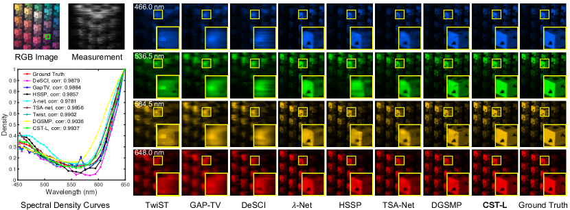
Figure 4: Reconstructed simulation HSI comparisons of Scene 2 with 4 out of 28 spectral channels. 7 SOTA methods and our CST-L are included. The spectral curves (bottom-left) are corresponding to the selected green box of the RGB image. Please zoom in.

5.2 Quantitative Results

Figure 5: CST vs. MST.

We compare the Params, FLOPS, PSNR, and SSIM of our CST and other SOTA methods, including three model-based methods (TwIST [3], GAP-TV [94], and DeSCI [50]), six CNN-based methods ($\lambda$-net [67], HSSP [81], DNU [82], PnP-DIP-HSI [66], TSA-Net [64], and DGSMP [37]), and a recent Transformer-based method (MST [6]). For fairness, we test all these algorithms with the same settings as [6, 37]. The results on 10 simulation scenes are reported in Tab. 1. As can be seen: (i) When we set the sparsity ratio to 0, our best model CST-L^∗ achieves very impressive results, i.e., 36.12 dB in PSNR and 0.957 in SSIM, showing the effectiveness of our method. (ii) Our CST families significantly outperform other SOTA algorithms while requiring cheaper computational costs. Particularly, when compared to the recent best Transformer-based method MST, our CST-S, CST-M, and CST-L achieve 0.45, 0.37, and 0.67 dB improvements while costing 1.29G, 1.16G, and 0.34G less FLOPS than MST-S, MST-M, and MST-L as shown in Fig. 5. When compared to CNN-based methods, our CST exhibits extreme efficiency advantages. For instance, CST-L outperforms DGSMP, TSA-Net, and $\lambda$-Net by 3.22, 4.39, and 7.32 dB while costing 79.8% (3.00 / 3.76), 6.8%, 4.8% Params and 4.3% (27.81 / 646.65), 25.3%, 23.6% FLOPS. Surprisingly, even our smallest model CST-S surpasses DGSMP, TSA-Net, and $\lambda$-Net by 2.08, 3.25, and 6.18 dB while requiring 31.9%, 2.7%, 1.9% Params and 1.8%, 10.6%, 9.9% FLOPS. These results demonstrate the cost-effectiveness superiority of our CST. This is mainly because CST embeds the HSI sparsity into the learning-based model, which reduces the inefficient computation of less informative dark regions and self-attention between content-unrelated tokens.

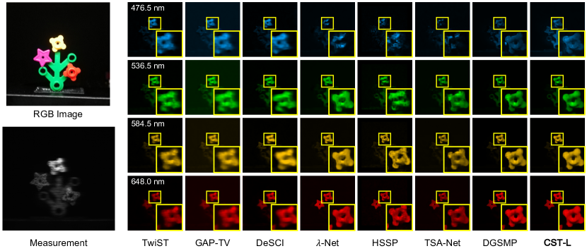
Figure 6: Reconstructed real HSI comparisons of Scene 1 with 4 out of 28 spectral channels. Seven SOTA algorithms and our CST-L are included. Our CST-L are more favorable to restore detailed contents and remove noise. Zoom in for a better view.

5.3 Qualitative Results

5.3.1 Simulation HSI Restoration.

Fig. 4 compares the restored simulation HSIs of our CST-L and seven SOTA algorithms on $Scene$ 2 with 4 out of 28 spectral channels. Please zoom in for better visualization. It can be observed from the reconstructed HSIs (right) and the zoomed-in patches in the yellow boxes that our CST is effective in producing perceptually pleasant images with more vivid sharp edge details while maintaining the spatial smoothness of the homogeneous regions without introducing artifacts. In contrast, other methods fail to restore fine-grained details. They either achieve over-smooth results sacrificing structural contents and high-frequency details, or generate blotchy textures and chromatic artifacts. Besides, Fig. 4 depicts the spectral density curves (bottom-left) corresponding to the selected region of the green box in the RGB image (top-left). Our curve achieves the highest correlation coefficient with the ground-truth curve. This evidence clearly demonstrates the spectral-dimension consistency reconstruction effectiveness of our proposed CST.

5.3.2 Real HSI Restoration.

We also evaluate our CST in real HSI reconstruction. Following the setting of [6, 37, 64], we re-train our CST-L with all samples of the KAIST and CAVE datasets. To simulate real CASSI, 11-bit shot noise is injected into the measurement during the training procedure. The reconstructed HSI comparisons are depicted in Fig. 6. Our CST-L shows significant advantages in fine-grained content restoration and real noise removal. These results verify the robustness, reliability, and generalization ability of our method.

Table 2: Ablations. Models are trained on CAVE and test on KAIST in simulation.

Method	Baseline	+ SAH-MSA	+ SASM
PSNR	32.57	35.53	35.31 ($\downarrow$ 0.60 %)
SSIM	0.906	0.948	0.947 ($\downarrow$ 0.10 %)
Params (M)	0.51	1.36	1.36  ($\downarrow$ 0.00 %)
FLOPS (G)	6.40	24.60	16.91 ($\downarrow$ 31.3 %)

(a) Break-down ablation study.

Method	Baseline	Random Sparsity	Uniform Sparsity	SASM
PSNR	32.57	34.37	34.33	35.31
SSIM	0.906	0.937	0.936	0.947
Params (M)	0.51	1.36	1.36	1.36
FLOPS (G)	6.40	16.89	16.89	16.91

(b) Ablation study of sparse mechanisms.

Method	Baseline	G-MSA	W-MSA	Swin-MSA	S-MSA	SAH-MSA
PSNR	32.57	35.04	35.02	35.12	35.21	35.53
SSIM	0.906	0.944	0.943	0.945	0.946	0.948
Params (M)	0.51	1.85	1.85	1.85	1.66	1.36
FLOPS (G)	6.40	35.58	24.98	24.98	24.74	24.60

(c) Ablation study of self-attention mechanisms.

Method	Baseline	Global	Local
PSNR	32.57	35.33	35.53
SSIM	0.906	0.946	0.948
Params (M)	0.51	1.36	1.36
FLOPS (G)	6.40	24.60	24.60

(d) Study of clustering scope.

5.4 Ablation Study

We adopt the simulation HSI datasets [18, 70] to conduct ablation studies. The baseline model is derived by removing our SAH-MSA and SASM from CST-M.

5.4.1 Break-down Ablation.

We firstly perform a break-down ablation to investigate the effect of each component and their interactions. The results are listed in Tab. 2a. The baseline model yields 32.57 dB in PSNR and 0.906 in SSIM. When SAH-MSA is applied, the performance gains by 2.96 dB in PSNR and 0.042 in SSIM, showing its significant contribution. When we continue to exploit SASM, the computational cost dramatically declines by 31.3% (7.69 / 24.60) while the performance only degrades by 0.6 % in PSNR and 0.1% in SSIM. This evidence suggests that our SASM can reduce the computational burden while sacrificing minimal reconstruction performance, thus increasing the model efficiency.

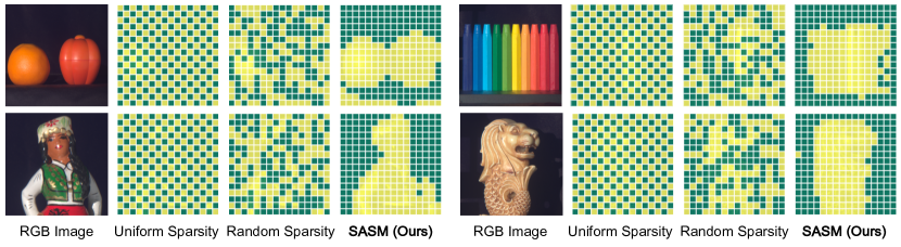
Figure 7: Visual analysis of uniform sparsity scheme, random sparsity scheme, and our SASM. We visualize the sparsity masks produced by different sparsity schemes. Yellow indicates the patch is selected while green means vice versa. Only our SASM can generate accurate response to the informative regions with HSI information.

5.4.2 Sparsity Scheme Comparison.

We conduct ablation to study the effects of sparsity schemes including: (i) random sparsity, i.e., the patches to be calculated are randomly selected, (ii) uniform sparsity, i.e., the patches to be calculated are uniformly distributed, and (iii) our SASM. The results are listed in Tab. 2b. Our SASM yields the best results and drastically outperforms other schemes (over 0.9 dB). Additionally, we conduct visual analysis of the sparsity mask generated by the three sparsity schemes. As depicted in Fig. 7, the sparsity mask produced by our SASM generates more complete and accurate responses to the informative regions with HSI information. In contrast, both random and uniform sparsity schemes are not aware of HSI signals and rigidly pick the preset positions. These results demonstrate the superiority of our SASM in perceiving spatially sparse HSI signals and locating regions with dense HSI representations.

5.4.3 Self-Attention Mechanism Comparison.

We compare our SAH-MSA with other self-attention mechanisms. The results are reported in Tab. 2c. The baseline yields 32.57 dB with 0.51 M Params and 6.40 G FLOPS. We respectively apply global MSA (G-MSA) [22], local window-based MSA (W-MSA) [52], Swin-MSA [52], spectral-wise MSA (S-MSA) [6], and SAH-MSA. The model gains by 2.47, 2.45, 2.55, 2.64, and 2.96 dB while adding 29.18, 18.58, 18.58, 18.34, and 18.20 G FLOPS and 1.34, 1.34, 1.34, 1.15, and 0.85 M Params. Our SAH-MSA yields the most significant improvement but requires the cheapest FLOPS and Params. Please note that we downscale the input feature of G-MSA into $\frac{1}{4}$ size to avoid memory bottlenecks. This evidence shows the cost-effectiveness advantage of SAH-MSA, which is mainly because SAH-MSA applies MSA calculation between tokens that are closely related in content within each $bucket$ while cutting down the burden of computation between content-uncorrelated elements.

5.4.4 Clustering Scope.

We study the effect of the scope of clustering, i.e., local vs. global. Local means constraining the hash clustering operation inside each $M\times M$ patch while global indicates applying the hash clustering to the whole image. In the beginning, we thought that expanding the receptive field would improve the performance. However, the experimental results in Tab. 2d point out the opposite. The model with local clustering scope performs better. We now analyze the reason for this observation. The hash clustering is essentially a linear dimension reduction ($h:\mathbb{R}^{C}\to\mathbb{Z}$) suffering from limited discriminative ability. It is suitable for simple, linearly separable situations with a small number of samples. When the clustering scope is enlarged from the local patch to the global image, the number of tokens increases dramatically ($M\times M\to H\times W$). As a result, the situation becomes more complex and may be linearly inseparable. Thus, the hash clustering performance degrades. Then the elements clustered into the same $bucket$ are less content-related and the MSA calculation of each $bucket$ becomes less effective, leading to the degradation of HSI restoration.

5.4.5 Parameter Analysis.

We adopt CST-M to conduct parameter analysis of sparsity rate $\sigma$, round number $R$ in Eq. (11), patch size $M$, and loss weight $\lambda$ in Eq. (6) as shown in Fig 8, where the vertical axis is PSNR and the circle radius is FLOPS. As can be observed: (i) When increasing $\sigma$, the computational cost declines but the performance is sacrificed. When $\sigma$ is larger than $50\%$, the performance degrades dramatically. (ii) When changing $R$ from 1 to 6, the reconstruction quality increases. Nonetheless, when $R\geq$ 2, further increasing $R$ does not lead to a significant improvement. (iii) The two maximums are achieved when $M$ = 16 and $\lambda$ = 2, respectively, without costing too much FLOPS. Since our goal is not to pursue the best results with heavy computational burden sacrificing the model efficiency but to yield a better trade-off between performance and computational cost, we finally set $\sigma$ = 0.5, $R$ = 2, $M$ = 16, and $\lambda$ = 2.

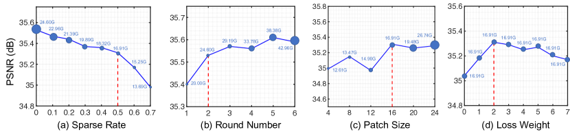
Figure 8: Parameter analysis of sparsity ratio $\sigma$, round number $R$, patch size $M$, and loss weight $\lambda$. The vertical axis is PNSR (in dB performance). The circle radius is FLOPS (computational cost). To achieve a better trade-off between performance and computational complexity, we finally set $\sigma$ = 0.5, $R$ = 2, $M$ = 16, and $\lambda$ = 2.

6 Conclusion

In this paper, we investigate a critical problem in HSI reconstruction, i.e., how to embed HSI sparsity into learning-based algorithms. To this end, we propose a novel Transformer-based method, named CST, for HSI restoration. CST firstly exploits SASM to detect informative regions with HSI representations. Then the detected patches are fed into our SAH-MSA to cluster spatially scattered tokens with closely correlated contents for calculating MSA. Extensive quantitative and qualitative experiments demonstrate that our CST significantly outperforms other SOTA methods while requiring cheaper computational costs. Additionally, our CST yields more visually pleasing results with more fine-grained details and structural contents than existing algorithms in real-world HSI reconstruction.

Acknowledgements: This work is partially supported by the NSFC fund (61831 014), the Shenzhen Science and Technology Project under Grant (JSGG20210802 153150005, CJGJZD20200617102601004), and the Westlake Foundation (2021B1 501-2). Xin Yuan would like to thank the funding from Lochn Optics.

References

- [1] Backman, V., Wallace, M.B., Perelman, L., Arendt, J., Gurjar, R., Muller, M., Zhang, Q., Zonios, G., Kline, E., McGillican, T.: Detection of preinvasive cancer cells. Nature (2000)
- [2] Bhojanapalli, S., Chakrabarti, A., Glasner, D., Li, D., Unterthiner, T., Veit, A.: Understanding robustness of transformers for image classification. In: ICCV (2021)
- [3] Bioucas-Dias, J., Figueiredo., M.: A new twist: Two-step iterative shrinkage/thresholding algorithms for image restoration. TIP (2007)
- [4] Borengasser, M., Hungate, W.S., Watkins, R.: Hyperspectral remote sensing: principles and applications. CRC press (2007)
- [5] Cai, Y., Hu, X., Wang, H., Zhang, Y., Pfister, H., Wei, D.: Learning to generate realistic noisy images via pixel-level noise-aware adversarial training. In: NeurIPS (2021)
- [6] Cai, Y., Lin, J., Hu, X., Wang, H., Yuan, X., Zhang, Y., Timofte, R., Gool, L.V.: Mask-guided spectral-wise transformer for efficient hyperspectral image reconstruction. In: CVPR (2022)
- [7] Cai, Y., Lin, J., Wang, H., Yuan, X., Ding, H., Zhang, Y., Timofte, R., Van Gool, L.: Degradation-aware unfolding half-shuffle transformer for spectral compressive imaging. arXiv preprint arXiv:2205.10102 (2022)
- [8] Cai, Y., Wang, Z., Luo, Z., Yin, B., Du, A., Wang, H., Zhou, X., Zhou, E., Zhang, X., Sun, J.: Learning delicate local representations for multi-person pose estimation. arXiv preprint arXiv:2003.04030 (2020)
- [9] Cao, J., Li, Y., Zhang, K., Van Gool, L.: Video super-resolution transformer. arXiv preprint arXiv:2106.06847 (2021)
- [10] Cao, X., Du, H., Tong, X., Dai, Q., Lin, S.: A prism-mask system for multispectral video acquisition. TPAMI (2011)
- [11] Cao, X., Yue, T., Lin, X., Lin, S., Yuan, X., Dai, Q., Carin, L., Brady, D.J.: Computational snapshot multispectral cameras: Toward dynamic capture of the spectral world. Signal Processing Magazine (2016)
- [12] Carion, N., Massa, F., Synnaeve, G., Usunier, N., Kirillov, A., Zagoruyko, S.: End-to-end object detection with transformers. In: ECCV (2020)
- [13] Chan, S.H., Wang, X., Elgendy, O.A.: Plug-and-play admm for image restoration: Fixed-point convergence and applications. Transactions on Computational Imaging (2016)
- [14] Chen, C.F.R., Fan, Q., Panda, R.: Crossvit: Cross-attention multi-scale vision transformer for image classification. In: ICCV (2021)
- [15] Chen, H., Wang, Y., Guo, T., Xu, C., Deng, Y., Liu, Z., Ma, S., Xu, C., Xu, C., Gao, W.: Pre-trained image processing transformer. In: CVPR (2021)
- [16] Chen, L.C., Papandreou, G., Schroff, F., Adam, H.: Rethinking atrous convolution for semantic image segmentation. arXiv preprint arXiv:1706.05587 (2017)
- [17] Cheng, B., Schwing, A., Kirillov, A.: Per-pixel classification is not all you need for semantic segmentation. In: NeurIPS (2021)
- [18] Choi, I., Kim, M., Gutierrez, D., Jeon, D., Nam, G.: High-quality hyperspectral reconstruction using a spectral prior. In: Technical report (2017)
- [19] Dai, X., Chen, Y., Yang, J., Zhang, P., Yuan, L., Zhang, L.: Dynamic detr: End-to-end object detection with dynamic attention. In: ICCV (2021)
- [20] Dai, Z., Cai, B., Lin, Y., Chen, J.: Up-detr: Unsupervised pre-training for object detection with transformers. In: CVPR (2021)
- [21] Deng, Z., Cai, Y., Chen, L., Gong, Z., Bao, Q., Yao, X., Fang, D., Zhang, S., Ma, L.: Rformer: Transformer-based generative adversarial network for real fundus image restoration on a new clinical benchmark. arXiv preprint arXiv:2201.00466 (2022)
- [22] Dosovitskiy, A., Beyer, L., Kolesnikov, A., Weissenborn, D., Zhai, X., Unterthiner, T., Dehghani, M., Minderer, M., Heigold, G., Gelly, S., Uszkoreit, J., Houlsby, N.: An image is worth 16x16 words: Transformers for image recognition at scale. In: ICLR (2021)
- [23] El-Nouby, A., Touvron, H., Caron, M., Bojanowski, P., Douze, M., Joulin, A., Laptev, I., Neverova, N., Synnaeve, G., Verbeek, J., et al.: Xcit: Cross-covariance image transformers. arXiv preprint arXiv:2106.09681 (2021)
- [24] Elad, M., Aharon, M.: Image denoising via learned dictionaries and sparse representation. In: CVPR (2006)
- [25] Fang, Y., Liao, B., Wang, X., Fang, J., Qi, J., Wu, R., Niu, J., Liu, W.: You only look at one sequence: Rethinking transformer in vision through object detection. In: NeurIPS (2021)
- [26] Fauvel, M., Tarabalka, Y., Benediktsson, J.A., Chanussot, J., Tilton, J.C.: Advances in spectral-spatial classification of hyperspectral images. Proceedings of the IEEE (2012)
- [27] Figueiredo, M.A., Nowak, R.D., Wright, S.J.: Gradient projection for sparse reconstruction: Application to compressed sensing and other inverse problems. IEEE Journal of selected topics in signal processing (2007)
- [28] Fu, Y., Liang, Z., You, S.: Bidirectional 3d quasi-recurrent neural network for hyperspectral image super-resolution. Journal of Selected Topics in Applied Earth Observations and Remote Sensing (2021)
- [29] Fu, Y., Zhang, T., Wang, L., Huang, H.: Coded hyperspectral image reconstruction using deep external and internal learning. TPAMI (2021)
- [30] Fu, Y., Zheng, Y., Sato, I., Sato, Y.: Exploiting spectral-spatial correlation for coded hyperspectral image restoration. In: CVPR (2016)
- [31] Gehm, M.E., John, R., Brady, D.J., Willett, R.M., Schulz, T.J.: Single-shot compressive spectral imaging with a dual-disperser architecture. Optics express (2007)
- [32] Han, K., Xiao, A., Wu, E., Guo, J., Xu, C., Wang, Y.: Transformer in transformer. In: NeurIPS (2021)
- [33] Hu, X., Cai, Y., Lin, J., Wang, H., Yuan, X., Zhang, Y., Timofte, R., Gool, L.V.: Hdnet: High-resolution dual-domain learning for spectral compressive imaging. In: CVPR (2022)
- [34] Hu, X., Cai, Y., Liu, Z., Wang, H., Zhang, Y.: Multi-scale selective feedback network with dual loss for real image denoising. In: IJCAI (2021)
- [35] Hu, X., Ma, R., Liu, Z., Cai, Y., Zhao, X., Zhang, Y., Wang, H.: Pseudo 3d auto-correlation network for real image denoising. In: CVPR (2021)
- [36] Hu, X., Wang, H., Cai, Y., Zhao, X., Zhang, Y.: Pyramid orthogonal attention network based on dual self-similarity for accurate mr image super-resolution. In: ICME (2021)
- [37] Huang, T., Dong, W., Yuan, X., Wu, J., Shi, G.: Deep gaussian scale mixture prior for spectral compressive imaging. In: CVPR (2021)
- [38] James, J.: Spectrograph design fundamentals. Cambridge University Press (2007)
- [39] Jiang, T., Camgoz, N.C., Bowden, R.: Skeletor: Skeletal transformers for robust body-pose estimation. In: CVPR (2021)
- [40] Kim, M.H., Harvey, T.A., Kittle, D.S., Rushmeier, H., J. Dorsey, R.O.P., Brady, D.J.: 3d imaging spectroscopy for measuring hyperspectral patterns on solid objects. ACM Transactions on on Graphics (2012)
- [41] Kingma, D.P., Ba, J.L.: Adam: A method for stochastic optimization. In: ICLR (2015)
- [42] Kitaev, N., Kaiser, Ł., Levskaya, A.: Reformer: The efficient transformer. arXiv preprint arXiv:2001.04451 (2020)
- [43] Lanchantin, J., Wang, T., Ordonez, V., Qi, Y.: General multi-label image classification with transformers. In: CVPR (2021)
- [44] Li, W., Liu, H., Ding, R., Liu, M., Wang, P.: Lifting transformer for 3d human pose estimation in video. arXiv preprint arXiv:2103.14304 (2021)
- [45] Li, X., Zhang, L., You, A., Yang, M., Yang, K., Tong, Y.: Global aggregation then local distribution in fully convolutional networks. In: BMVC (2019)
- [46] Li, Y., Hao, M., Di, Z., Gundavarapu, N.B., Wang, X.: Test-time personalization with a transformer for human pose estimation. In: NeurIPS (2021)
- [47] Liang, J., Cao, J., Sun, G., Zhang, K., Van Gool, L., Timofte, R.: Swinir: Image restoration using swin transformer. In: ICCVW (2021)
- [48] Lin, J., Cai, Y., Hu, X., Wang, H., Yan, Y., Zou, X., Ding, H., Zhang, Y., Timofte, R., Van Gool, L.: Flow-guided sparse transformer for video deblurring. arXiv preprint arXiv:2201.01893 (2022)
- [49] Lin, K., Wang, L., Liu, Z.: End-to-end human pose and mesh reconstruction with transformers. In: CVPR (2021)
- [50] Liu, Y., Yuan, X., Suo, J., Brady, D., Dai, Q.: Rank minimization for snapshot compressive imaging. TPAMI (2019)
- [51] Liu, Y., Yuan, X., Suo, J., Brady, D.J., Dai, Q.: Rank minimization for snapshot compressive imaging. TPAMI (2018)
- [52] Liu, Z., Lin, Y., Cao, Y., Hu, H., Wei, Y., Zhang, Z., Lin, S., Guo, B.: Swin transformer: Hierarchical vision transformer using shifted windows. In: ICCV (2021)
- [53] Loshchilov, I., Hutter, F.: Sgdr: Stochastic gradient descent with warm restarts. arXiv preprint arXiv:1608.03983 (2016)
- [54] Lu, G., Fei, B.: Medical hyperspectral imaging: a review. Journal of Biomedical Optics (2014)
- [55] Lu, Z., He, S., Zhu, X., Zhang, L., Song, Y.Z., Xiang, T.: Simpler is better: Few-shot semantic segmentation with classifier weight transformer. In: ICCV (2021)
- [56] Ludwig, K., Harzig, P., Lienhart, R.: Detecting arbitrary intermediate keypoints for human pose estimation with vision transformers. In: WACV (2022)
- [57] Ma, J., Liu, X.Y., Shou, Z., Yuan, X.: Deep tensor admm-net for snapshot compressive imaging. In: ICCV (2019)
- [58] Maggiori, E., Charpiat, G., Tarabalka, Y., Alliez, P.: Recurrent neural networks to correct satellite image classification maps. Transactions on Geoscience and Remote Sensing (2017)
- [59] Manakov, A., Restrepo, J., Klehm, O., Hegedus, R., Eisemann, E., Seidel, H.P., Ihrke, I.: A reconfigurable camera add-on for high dynamic range, multispectral, polarization, and light-field imaging. Transactions on Graphics (2013)
- [60] Mao, W., Ge, Y., Shen, C., Tian, Z., Wang, X., Wang, Z.: Tfpose: Direct human pose estimation with transformers. arXiv preprint arXiv:2103.15320 (2021)
- [61] Mei, Y., Fan, Y., Zhou, Y.: Image super-resolution with non-local sparse attention. In: CVPR (2021)
- [62] Melgani, F., Bruzzone, L.: Classification of hyperspectral remote sensing images with support vector machines. Transactions on geoscience and remote sensing (2004)
- [63] Meng, Z., Jalali, S., Yuan, X.: Gap-net for snapshot compressive imaging. arXiv preprint arXiv:2012.08364 (2020)
- [64] Meng, Z., Ma, J., Yuan, X.: End-to-end low cost compressive spectral imaging with spatial-spectral self-attention. In: ECCV (2020)
- [65] Meng, Z., Qiao, M., Ma, J., Yu, Z., Xu, K., Yuan, X.: Snapshot multispectral endomicroscopy. Optics Letters (2020)
- [66] Meng, Z., Yu, Z., Xu, K., Yuan, X.: Self-supervised neural networks for spectral snapshot compressive imaging. In: ICCV (2021)
- [67] Miao, X., Yuan, X., Pu, Y., Athitsos, V.: l-net: Reconstruct hyperspectral images from a snapshot measurement. In: ICCV (2019)
- [68] Misra, I., Girdhar, R., Joulin, A.: An end-to-end transformer model for 3d object detection. In: ICCV (2021)
- [69] Pan, X., Xia, Z., Song, S., Li, L.E., Huang, G.: 3d object detection with pointformer. In: CVPR (2021)
- [70] Park, J.I., Lee, M.H., Grossberg, M.D., Nayar, S.K.: Multispectral imaging using multiplexed illumination. In: ICCV (2007)
- [71] Patrick, W., Hirsch, M., Scholkopf, B., Lensch, H.P.A.: Learning blind motion deblurring. In: ICCV (2017)
- [72] Qiao, M., Liu, X., Yuan, X.: Snapshot spatial–temporal compressive imaging. Optics letters (2020)
- [73] Ramachandran, P., Parmar, N., Vaswani, A., Bello, I., Levskaya, A., Shlens, J.: Stand-alone self-attention in vision models. In: NeurIPS (2019)
- [74] Solomon, J., Rock, B.: Imaging spectrometry for earth remote sensing. Science (1985)
- [75] Strudel, R., Garcia, R., Laptev, I., Schmid, C.: Segmenter: Transformer for semantic segmentation. In: ICCV (2021)
- [76] Uzkent, B., Hoffman, M.J., Vodacek, A.: Real-time vehicle tracking in aerial video using hyperspectral features. In: CVPRW (2016)
- [77] Uzkent, B., Rangnekar, A., Hoffman, M.: Aerial vehicle tracking by adaptive fusion of hyperspectral likelihood maps. In: CVPRW (2017)
- [78] Vaswani, A., Shazeer, N., Parmar, N., Uszkoreit, J., Jones, L., Gomez, A.N., Kaiser, Ł., Polosukhin, I.: Attention is all you need. In: NeurIPS (2017)
- [79] Wagadarikar, A., John, R., Willett, R., Brady, D.: Single disperser design for coded aperture snapshot spectral imaging. Applied optics (2008)
- [80] Wang, L., Wu, Z., Zhong, Y., Yuan, X.: Spectral compressive imaging reconstruction using convolution and spectral contextual transformer. arXiv preprint arXiv:2201.05768 (2022)
- [81] Wang, L., Sun, C., Fu, Y., Kim, M.H., Huang, H.: Hyperspectral image reconstruction using a deep spatial-spectral prior. In: CVPR (2019)
- [82] Wang, L., Sun, C., Zhang, M., Fu, Y., Huang, H.: Dnu: Deep non-local unrolling for computational spectral imaging. In: CVPR (2020)
- [83] Wang, L., Xiong, Z., Gao, D., Shi, G., Wu, F.: Dual-camera design for coded aperture snapshot spectral imaging. Applied optics (2015)
- [84] Wang, Z., Cun, X., Bao, J., Liu, J.: Uformer: A general u-shaped transformer for image restoration. arXiv preprint 2106.03106 (2021)
- [85] Wang, Z., Bovik, A.C., Sheikh, H.R., Simoncell, E.P.: Image quality assessment: from error visibility to structural similarity. TIP (2004)
- [86] Wu, B., Xu, C., Dai, X., Wan, A., Zhang, P., Yan, Z., Tomizuka, M., Gonzalez, J., Keutzer, K., Vajda, P.: Visual transformers: Token-based image representation and processing for computer vision. arXiv preprint arXiv:2006.03677 (2020)
- [87] Wu, K., Peng, H., Chen, M., Fu, J., Chao, H.: Rethinking and improving relative position encoding for vision transformer. In: ICCV (2021)
- [88] Xie, E., Wang, W., Yu, Z., Anandkumar, A., Alvarez, J.M., Luo, P.: Segformer: Simple and efficient design for semantic segmentation with transformers. In: NeurIPS (2021)
- [89] Xiong, Z., Shi, Z., Li, H., Wang, L., Liu, D., Wu, F.: Hscnn: Cnn-based hyperspectral image recovery from spectrally undersampled projections. In: ICCVW (2017)
- [90] Yang, J., Wang, Z., Lin, Z., Cohen, S., Huang, T.: Coupled dictionary training for image super-resolution. TIP (2012)
- [91] Yang, J., Wright, J., Huang, T.S., Ma, Y.: Image super-resolution via sparse representation. TIP (2010)
- [92] Yang, J., Li, C., Zhang, P., Dai, X., Xiao, B., Yuan, L., Gao, J.: Focal self-attention for local-global interactions in vision transformers. arXiv preprint arXiv:2107.00641 (2021)
- [93] Yang, Z., Wei, Y., Yang, Y.: Associating objects with transformers for video object segmentation. In: NeurIPS (2021)
- [94] Yuan, X.: Generalized alternating projection based total variation minimization for compressive sensing. In: ICIP (2016)
- [95] Yuan, X., Liu, Y., Suo, J., Dai, Q.: Plug-and-play algorithms for large-scale snapshot compressive imaging. In: CVPR (2020)
- [96] Yuan, Y., Zheng, X., Lu, X.: Hyperspectral image superresolution by transfer learning. Journal of Selected Topics in Applied Earth Observations and Remote Sensing (2017)
- [97] Yuan, Y., Fu, R., Huang, L., Lin, W., Zhang, C., Chen, X., Wang, J.: Hrformer: High-resolution transformer for dense prediction. In: NeurIPS (2021)
- [98] Zamir, S.W., Arora, A., Khan, S., Hayat, M., Khan, F.S., Yang, M.H.: Restormer: Efficient transformer for high-resolution image restoration. ArXiv 2111.09881 (2021)
- [99] Zamir, S.W., Arora, A., Khan, S., Hayat, M., Khan, F.S., Yang, M.H., Shao, L.: Cycleisp: Real image restoration via improved data synthesis. In: CVPR (2020)
- [100] Zamir, S.W., Arora, A., Khan, S., Hayat, M., Khan, F.S., Yang, M.H., Shao, L.: Learning enriched features for real image restoration and enhancement. In: ECCV (2020)
- [101] Zamir, S.W., Arora, A., Khan, S., Hayat, M., Khan, F.S., Yang, M.H., Shao, L.: Multi-stage progressive image restoration. In: CVPR (2021)
- [102] Zhang, F., Du, B., Zhang, L.: Scene classification via a gradient boosting random convolutional network framework. Transactions on Geoscience and Remote Sensing (2015)
- [103] Zhang, Y., Li, K., Li, K., Wang, L., Zhong, B., Fu, Y.: Image super-resolution using very deep residual channel attention networks. In: ECCV (2018)
- [104] Zhang, Y., Li, K., Li, K., Zhong, B., Fu, Y.: Residual non-local attention networks for image restoration. In: ICLR (2019)
- [105] Zhao, C., Zhang, J., Ma, S., Fan, X., Zhang, Y., Gao, W.: Reducing image compression artifacts by structural sparse representation and quantization constraint prior. TCSVT (2016)
- [106] Zheng, C., Zhu, S., Mendieta, M., Yang, T., Chen, C., Ding, Z.: 3d human pose estimation with spatial and temporal transformers. In: ICCV (2021)
- [107] Zheng, S., Lu, J., Zhao, H., Zhu, X., Luo, Z., Wang, Y., Fu, Y., Feng, J., Xiang, T., Torr, P.H., Zhang, L.: Rethinking semantic segmentation from a sequence-to-sequence perspective with transformers. In: CVPR (2021)
- [108] Zhu, X., Su, W., Lu, L., Li, B., Wang, X., Dai, J.: Deformable detr: Deformable transformers for end-to-end object detection. In: ICLR (2021)