Bayesian Multi-Arm De-Intensification Designs

Abstract

In recent years new cancer treatments improved survival in multiple histologies. Some of these therapeutics, and in particular treatment combinations, are often associated with severe treatment-related adverse events (AEs). It is therefore important to identify alternative de-intensified therapies, for example dose-reduced therapies, with reduced AEs and similar efficacy. We introduce a sequential design for multi-arm de-intensification studies. The design evaluates multiple de-intensified therapies at different dose levels, one at the time, based on modeling of toxicity and efficacy endpoints. We study the utility of the design in oropharynx cancer de-intensification studies. We use a Bayesian nonparametric model for efficacy and toxicity outcomes to define decision rules at interim and final analysis. Interim decisions include early termination of the study due to inferior survival of experimental arms compared to the standard of care (SOC), and transitions from one de-intensified treatment arm to another with a further reduced dose when there is sufficient evidence of non-inferior survival. We evaluate the operating characteristics of the design using simulations and data from recent de-intensification studies in human papillomavirus (HPV)-associated oropharynx cancer.

Keywords: Bayesian design, De-intensification study, Multi-arm study

1 Introduction

In the last two decades several new cancer treatments have improved patient survival [39]. A large portion of new therapies consists of a backbone treatment, often chemotherapy or radiation therapy, combined with an additional drug, for example a targeted therapy or an immune checkpoint inhibitor. Some of these combination therapies improved survival, but they are associated with severe AEs. Intensity-modulated radiotherapy (IMRT) in combination with cisplatin is a SOC in oropharynx cancer [1] with three year survival rates close to 90% [1, 15]. However, the addition of cisplatin to IMRT is associated with a substantial increase in acute and late AEs compared with IMRT alone [30]. Similarly, a combination treatment including chemotherapy is the SOC for early-stage HER2-positive breast cancer and it has a high rate of treatment-related AEs [27].

AEs associated with new anticancer treatments are the main motivation for testing if de-intensified therapies maintain efficacy similar to the SOC and reduce treatment related AEs. For instance, the recent studies E1308[26], OPTIMA[37], RTOG1016 [15], DeEscalate[28], PAMELA [25] and KRISTINE [18] evaluated de-intensified therapies in oropharynx cancer and breast cancer. De-intensification studies consider therapies that (i) are dose reductions of SOC therapies, (ii) replace one component of the SOC combination therapy with a potentially less toxic drug, or (iii) eliminate the backbone treatment from the SOC. In all these cases the clinical study seeks to demonstrate that the de-intensified treatment has survival outcomes similar to the SOC and reduces AEs.

The design that we introduce is motivated by a clinical study in HPV-associated oropharynx cancer at our institution. HPV is a DNA onco-virus [14]. HPV positive and negative oropharynx cancer constitute distinct cancer sub-types with distinct molecular characteristics and epidemiological profiles [14]. Several ongoing clinical studies are evaluating de-intensified therapies [29]. The trial that we designed will evaluate two de-intensified therapies which differ in the IMRT dose levels.

Two large de-intensification studies RTOG1016[15] and De-ESCALaTE [28], which replaced cisplatin with the EGFR inhibitor cetuximab, recently reported inferior survival under the de-intensified therapy compared to the SOC (estimated overall survival hazard ratios of 1.45 and 5 for RTOG1016 and De-ESCALaTE) without reducing AEs. De-intensified studies in HPV-associated oropharynx cancer tend to use large margins [5] for testing non-inferiority to reduce sample sizes at targeted type I/II error rates. These margins and inadequate interim analyses can lead - as the results of RTOG1016 and De-ESCALaTE suggest - to a large number of patients exposed to treatments with reduced efficacy. This indicates the importance of sequential de-intensification designs to handle trade-offs between power and the number of patients exposed to inferior and toxic treatments using adequate interim analyses (IAs).

We introduce a Bayesian design for de-intensification studies. The design allows investigators to test multiple treatments sequentially, for instance two de-intensified treatments with $80\%$ and $40\%$ of the original IMRT dose of the SOC. Using a Bayesian nonparametric model for the distribution of survival times and AEs we specify sequential decision rules to evaluate treatment response and toxicity reductions. These include early stopping rules that are tuned to balance (i) the risk of patients receiving inferior treatments that reduce survival and (ii) the need to identify non-inferior de-intensified treatments that reduce toxicities. The multi-arm design evaluates de-intensified therapies one at the time starting from dose-levels close to the SOC, with subsequent arms at lower dose-levels tested only if there is evidence of non-inferiority and reductions of AEs for the previous de-intensified treatments.

We discuss algorithms to tune stopping rules accordingly to pre-defined early stopping probabilities under the null hypothesis of inferior survival or AEs identical to the SOC. Additionally the design calibrates the type I error rate to approximately match a targeted $\alpha$-level. We evaluate the operating characteristics of the design using data from recent de-intensification trials in HPV-associated oropharynx cancer.

De-intensification designs use non-inferiority (NI) testing procedures with a pre-defined NI margin and evaluate if the efficacy of an experimental treatment is comparable to the SOC [5]. Statistical considerations for NI studies concern the selection of a suitable testing procedure, the specification of the NI margin $\Delta$, and the study design, including early stopping rules and the selection of the sample size [2, 35, 11, 21, 22]. [2] discussed NI tests based on asymptotic techniques and [8, 42, 24] focused on the finite-sample operating characteristics of NI tests. Exact NI tests have been discussed in [3, 24], and extensions to time-to-event outcomes have been proposed in [35, 11]. Other contributions focused on the selection of suitable NI margins $\Delta$ [41, 17] and on the specification of early stopping rules for sequential NI experiments [10, 23, 22].

Bayesian work on NI experiments includes NI testing methodologies and the use of data from previous clinical studies in the analysis of NI experiments [40, 36]. [45] and [46] discussed NI tests for binary endpoints using beta prior distributions, and [32] proposed the use of Bernstein priors. [13] used Bayesian modeling to select the NI margin $\Delta$ and [6, 4] investigated Bayesian sample size calculations for single-stage NI tests.

The main difference between these non-sequential single-stage non-inferiority testing procedures and our work is that we introduce a sequential design for de-intensification studies with efficacy and toxicity co-primary endpoints. The design utilizes a non-parametric Bayesian model to analyze survival data and AEs during the study. Key decision to pause, stop or continue the evaluation of de-intensified treatments, are based on data summaries that quantify the trade-off between the risk of exposing patients to an inferior treatment and the likelihood of demonstrating relevant reductions of AEs.

The outline of the paper is as follows. After introducing some notation in Section 2, we present the de-intensification design for studies with efficacy endpoints (Section 2.1) and for studies with efficacy and toxicity co-primary endpoints (Section 2.2). Section 3 summarizes the Bayesian probability model that we used. In Section 4.1 we evaluate the operating characteristics of the trial design under different design parameters. Section 4.2 compares several de-intensification strategies in HPV-associated oropharynx cancer with efficacy endpoints. Section 4.3 extends this comparison to oropharynx cancer studies with efficacy and toxicity co-primary endpoints.

2 De-intensification design

We consider a phase II clinical study with $k=1,\cdots,K$ de-intensified treatments. We assume the study does not include a control arm. Simple modifications of the design that we discuss allow to include a control arm. In the de-escalation setting, the SOC ($k=0$) survival distribution has been estimated previously and the SOC is associated with a substantial risk of AEs. De-intensified treatments $k=1,\cdots,K$ are likely to present better toxicity profiles (i.e. reduced doses of the backbone treatment), but may reduce patients’ survival. In practice $K=2$ or $3$. $K=2$ in our study at DFCI.

We evaluate if one or multiple treatments $k$ are non-inferior compared to the SOC and reduce AEs. De-intensified treatments are ranked. For example, if $k=1,\cdots,K$ are de-intensified dose levels, the study starts testing the highest dose ($k=1$), followed by further dose reductions $k=2,\ldots,K$.

A maximum of $n$ patients are enrolled. For each patient $1\leq i\leq n,$ $(T_{i},C_{i},Y_{i},X_{i})$ indicates the assignment to arm $C_{i}\in\{1,\cdots,K\}$ at enrollment time $T_{i}\geq 0$, and $Y_{i}$ and $X_{i}$ are the efficacy and toxicity outcomes. In our study, $Y_{i}$ indicates the progression free survival (PFS) time and $X_{i}$ is the time of the first treatment-related AE (grade $\geq$3). $F_{k}(\cdot)$ and $G_{k}(\cdot)$ indicate the distributions of $Y_{i}$ and $X_{i}$ for patients on treatment $k$, and $n_{t,k}$ and $n_{t}$ are the number of enrollments to arm $k$ and total number of enrollments at time $t$. Lastly, $\Sigma_{t}$ denotes the data collected until time $t$ since the first enrollment.

In some cases AEs reductions of treatments $k$ compared to the SOC can be anticipated or have been demonstrated before the de-escalation study, while in other cases it is necessary to estimate both toxicity and efficacy during the trial. Therefore we first introduce in Section 2.1 a design for clinical studies that utilize only survival outcomes for interim and final decisions, and then extend in Section 2.2 the design to include both toxicity and efficacy co-primary endpoints. The designs can be combined with any Bayesian model for the unknown distributions $F_{k}(\cdot)$ and $G_{k}(\cdot)$.

2.1 De-intensification studies with efficacy primary outcomes

For each de-intensified treatment $k$, efficacy is quantified by a summary $\theta_{k}=\theta(F_{k})\in\mathbb{R}$. A large $\theta_{k}$ corresponds to a large treatment effect. Examples include the median, or the restricted mean survival time (RMST) $E[\min(Y_{i},t_{E})|C_{i}=k,F_{k}]$ at a pre-specified $t_{E}>0$.

For each $k=1,\cdots,K$ the null and alternative hypotheses that we consider are

$$\mathcal{H}_{0,k}=\{\theta_{k}\in\mathbb{R}:\theta_{k}\leq\theta_{0}-\Delta\}~{}~{}\text{ and }~{}~{}\mathcal{H}_{A,k}=\{\theta_{k}\in\mathbb{R}:\theta_{k}>\theta_{0}-\Delta_{k}\}.$$ (1)

Here $\Delta\geq\Delta_{k}>0$ are pre-specified margins. Values of $\theta_{k}$ below $\theta_{0}-\Delta$ make arm $k$ inferior, whereas $\theta_{k}\geq\theta_{0}-\Delta_{k}$ indicates an attractive alternative to the SOC. The design evaluates treatments sequentially (we will consider $K=2$), one after another, starting with arm $k=1$, which is less likely to be inferior than the others.

Figure 1 illustrates the design and a list of possible decisions at interim analyses (IAs). A maximum of $m_{\max}\leq n$ patients will be assigned to each treatment and a minimum of $m_{NI}\leq m_{\max}$ enrollments to treatment $k$ are required before it can be declared non-inferior. At regular time intervals $t=1,2,\cdots,$ (e.g. monthly or quarterly) IAs are conducted, and the active experimental arm $k$ may be (Panel B of Figure 1)

• declared non-inferior to the SOC, and the trial progresses to evaluate treatment $k+1$,

• declared inferior to the SOC and the study terminates, or

• enrollment to treatment $k$ continues, or

• enrollment is paused for a maximum follow-up time $t_{FU}$ since the last enrollment to arm $k$, to allow the accumulation of sufficient information for testing $\mathcal{H}_{0,k}$.

Figure 1: Schematic representation of the trial design with $K=2$ treatments. See Section 2.2 for the integrated use of efficacy and toxicity co-primary endpoints.

Parameter
$m_{\max}$	maximum number of enrollments per arm
$m_{I},m_{T},m_{NI}$	minimum number of enrollments to treatment k before arm $k$ can be stopped
	for inferiority ($m_{I}$) or toxicity ($m_{T}$), and $\mathcal{H}_{0,k}$ can be rejected ($m_{NI}$)
$\Delta,\Delta_{L},\Delta_{k}$	margins used for testing non-inferiority and for early futility stoping
$\Delta_{\beta}$	margin used for early stopping due to insufficient toxicity reductions
$b_{j}(\cdot),S_{j},s_{j}$	non-inferiority ($j=NI$), inferiority $(j=I)$ and toxicity $(j=T)$ boundary $b_{j}(\cdot)$,
	with shape and scale parameters $S_{j}$ and $s_{j}$
$p_{I},p_{T}$	$s_{j},j=I,T$ are selected so that a proportion of $p_{I}$ and $p_{T}$ trials are
	stopped early at IAs when treatment $k$ has inferior survival ($p_{I}$)
	or does not reduce toxicities $(p_{T})$

Table 1: Summary of parameters in the de-intensification designs with efficacy primary endpoint (Sections 2.1), and efficacy and toxicity co-primary endpoints (Sections 2.2).

Let $D_{t}=(D_{t,1},D_{t,2})$ indicate the de-intensified treatment $D_{t,1}\in\{\emptyset,1,\ldots,K\}$ that is evaluated between IAs $t$ and $t+1$ ($\emptyset$ if the study is terminated at IA $t$), and $D_{t,2}\in\{d_{E},d_{P},d_{T}\}$ denotes the status of the study during this time interval, where $d_{E}=$”enrollment is open”, $d_{P}=$ ”enrollment is paused ”, and $d_{T}=$ ”the study has been terminated” (Figure 1).

Stopping rules: Let $b_{I}(\cdot)$ be a predefined futility stopping-boundary with $1\geq b_{I}(n_{t,k})\geq 0$ (see Section 2.1.1 for details). Let $D_{t-1}=(k,d_{E})$ between IA $t-1$ and $t$. Arm $k$ is stopped for futility at IA $t$ if the probability of low efficacy becomes larger than $b_{I}(n_{t,k})$, i.e. if

$$p(\theta_{k}\leq\theta_{0}-\Delta_{k}|\Sigma_{t})>b_{I}(n_{t,k}),$$ (2)

and the study is terminated, $D_{t}=(\emptyset,d_{T}).$

If there is evidence of non-inferiority

$$p(\theta_{k}>\theta_{0}-\Delta|\Sigma_{t})>b_{NI}(n_{t,k}),$$ (3)

arm $k$ is declared non-inferior to the SOC. Here $0\leq b_{NI}(n_{t,k})\leq 1$ is a pre-specified non-inferiority stopping boundary. If there is evidence of non-inferiority according to (3), the study proceeds to treatment $k+1$ conditionally on the availability of a sufficient sample size $n_{t}\leq n-m_{\max}$, i.e. $D_{t}=(k+1,d_{E})$. Otherwise, the study is terminated, $D_{t}=(\emptyset,d_{T})$.

Pause enrollment: If the probabilities in (3) and (2) don’t cross the stopping boundaries, then enrollment to arm $k$ continues, $D_{t}=(k,d_{E})$, unless the maximum enrollment per arm $m_{\max}$ has been reached. When $n_{t,k}=m_{\max}$, enrollment is paused, i.e. $D_{t}=(k,d_{P})$, until treatment $k$ is declared non-inferior or inferior according to (2) and (3) at later IAs, or until the follow-up time $t_{FU}$ since the last enrollment is reached. This potential pause is necessary before testing arm $k+1$ to limit patients’ exposure to inferior treatments. If the probabilities in (3) don’t cross the stopping boundaries by the end of the follow-up period $t_{FU}$, the study closed and the null hypothesis $\mathcal{H}_{0,1}$ is not rejected.

2.1.1 Calibration of the design thresholds

We use functions $b_{j}(\cdot),j=I$ or $NI$, of the form

$$b_{j}(\ell)=1-s_{j}\times\max\bigg{[}0,\dfrac{\ell-m_{j}}{m_{\max}-m_{j}}\bigg{]}^{S_{j}}\text{ for }\ell=1,2,\cdots,m_{\max}.$$ (4)

The parameter $S_{j}\geq 0$ determines the shape of $b_{j}(\cdot),j=NI,I$, which is decreasing from 1 to $(1-s_{j})\in[0,1]$ when $S_{j}>0$ and constant $b_{j}(n)=1-s_{j}$ for $m_{j}\leq n\leq m_{\max}$ when $S_{j}=0$. Here $m_{NI}$ and $m_{I}$ indicate the minimum number of enrollments necessary before $\mathcal{H}_{0,k}$ can be rejected and before early futility stopping.

We fix $\mathcal{S}=(s_{I},S_{I},S_{NI},m_{NI},m_{I})$ (see Section 4.1 for a discussion on the selection of these parameters), and calibrate the parameter $s_{NI}$ of the boundary $b_{NI}(\cdot)$ that bounds the type I error rate at the desired $\alpha$ level across a set $\mathcal{F}_{I}$ of inferior (I) scenarios that satisfy $\theta(F)=\theta_{0}-\Delta$ for each $F\in\mathcal{F}_{I}$.

Scenarios: We use the historical control $F_{0}$ (published Kaplan-Meier estimator) and select a set of transformations $F=g(F_{0})$ (proportional hazards, accelerated failure time, proportional odds, etc.) such that $\theta(F)=\theta_{0}-\Delta$ for each $F$ in $\mathcal{F}_{I}$.

Controlling the type I error rate: For each $F\in\mathcal{F}_{I}$, we determine the largest value of $s_{NI,F}$ that bounds the designs’ type I error rate for arm 1 at level $\alpha$ when $F_{1}=F$. We then set $s_{NI}=\min_{F\in\mathcal{F}_{I}}s_{NI,F}.$ Relevant operating characteristics, such as power and the average study duration, depends on the selected $\mathcal{S},$ and in Section 4.1 we discuss the selection of these parameters.

Calibration. We estimate $s_{NI,F}$ using a Monte-Carlo procedure, by simulating $C$ trials (we use $C=2000$ in Section 4) with individual outcomes generated from $F$ and random enrollment times (with a fixed enrollment rate) of $m_{\max}$ patients. For each simulation $c=1,\cdots,C$, we compute the number of enrollments $n^{(c)}_{t,1}$ by IA $t=1,2,\ldots,$ and the posterior probabilities $U^{(c)}_{I,t}$ and $U^{(c)}_{NI,t}$ to declare inferiority ($U^{(c)}_{I,t}$) in (2) and non-inferiority ($U^{(c)}_{NI,t}$) in (3). Since $U^{(c)}_{NI,t}>b_{NI}(n^{(c)}_{t,1})$ in (3) is equivalent to $s_{NI}<s^{(c)}_{t}$, where

$$s^{(c)}_{t}=\Big{(}1-U^{(c)}_{NI,t}\Big{)}\Big{/}\max\bigg{[}0,\dfrac{n^{(c)}_{t,1}-m_{NI}}{m_{\max}-m_{NI}}\bigg{]}^{S_{NI}},$$

the simulated trial $c$ does not reject the null hypothesis $\mathcal{H}_{0,1}$ (at time $t$, or at any other interim analysis) if $s_{NI}$ is larger or equal than $\displaystyle s^{(c)}_{NI}=\min s_{t}^{(c)}$ where the minimum is over all $t$ such that $U^{(c)}_{I,t^{\prime}}<b_{I}(n^{(c)}_{t^{\prime},1})\text{ for }t^{\prime}\leq t$. We then estimate $s_{NI,F}$ as the $\alpha$-percentile of $\{s^{(c)}_{NI}\}_{c=1}^{C}$.

2.2 Efficacy and toxicity co-primary outcomes

When little is known about AEs of the de-intensified treatments, it becomes necessary to evaluate AEs together with efficacy as co-primary endpoints. Recall that $X_{i}$ indicates the time (months since enrollment) of the first AE (grade $\geq 3$) for patient $i$, with distribution function $G_{k}$ for arm $k$, and $\beta_{k}$ is a toxicity summary. Small values of $\beta_{k}$ indicate high toxicity. In Section 4.3 we use the RMST $\beta_{k}=E[\min(X_{i},t_{E})|C_{i}=k,G_{k}]$.

We consider the null and alternative hypotheses

$$\mathcal{H}_{0,k} =\{(\theta_{k},\beta_{k})\in\mathbb{R}^{2}:\theta_{k}\leq\theta_{0}-\Delta\text{ or }\beta_{k}\leq\beta_{0}\},\text{ and }$$

$$\mathcal{H}_{A,k} =\{(\theta_{k},\beta_{k})\in\mathbb{R}^{2}:\theta_{k}>\theta_{0}-\Delta\text{ and }\beta_{k}>\beta_{0}+\Delta_{\beta}\},$$

where $\Delta_{\beta}>0$, and extend the design in Section 2.1 to include toxicity outcomes.

Stopping rules: Treatment $k$, at time $t\geq 1$, is declared non-inferior and less toxic than the SOC if the posterior probability of $\mathcal{H}_{A,k}$ crosses a pre-specified boundary $b_{NI}(n_{t,k})$, i.e.

$$p\big{(}\{\theta_{k}>\theta_{0}-\Delta\}\cap\{\beta_{k}>\beta_{0}\}|\Sigma_{t}\big{)}\geq b_{NI}(n_{t,k}).$$

The function $b_{NI}(\cdot)$ and the futility boundaries introduced below belong to the same parametric family (4). When $\mathcal{H}_{0,k}$ is rejected the trial proceeds to enroll patients to arm $k+1$ if the sample size $n_{t}\leq n-m_{\max}$, otherwise the study terminates.

We extend the early termination rules for inferiority to include toxicities. Specifically, arm $k$ is stopped due to insufficient early evidence of toxicity reductions if the posterior probability of the event $\{\beta_{k}\leq\beta_{0}+\Delta_{\beta}\}$, for $\Delta_{\beta}\in\mathbb{R}$, exceeds the toxicity boundary $b_{T}(n_{t,k})$, i.e. $p\big{(}\beta_{k}\leq\beta_{0}+\Delta_{\beta}|\Sigma_{t}\big{)}>b_{T}(n_{t,k}).$

Additionally, therapy $k$ can be stopped for inferiority, if the posterior probability of the event $\{\theta_{k}\leq\theta_{0}-\Delta_{k}\}$ becomes larger than the boundary $b_{I}(n_{t,k})$. The margin $\Delta_{k}=\Delta_{k}(\Sigma_{t})$ now depends on the current evidence of toxicity reductions i.e. a function of the available toxicity data, and can vary during the study. In particular, with low evidence of toxicity reductions we use a smaller margin than in presence of strong evidence of relevant toxicity reductions,

$$\Delta_{k}(\Sigma_{t})=\begin{cases}\Delta&\text{ if }p\big{(}\beta_{k}\leq\beta_{0}+\Delta_{\beta}|\Sigma_{t}\big{)}\in(0,B_{T}(n_{t,k})],\\ \Delta_{L}&\text{ if }p\big{(}\beta_{k}\leq\beta_{0}+\Delta_{\beta}|\Sigma_{t}\big{)}\in(B_{T}(n_{t,k}),1],\end{cases}$$ (5)

where $\Delta\geq\Delta_{L},$ $B_{T}(n_{t,k})<b_{T}(n_{t,k}),$ and $B_{T}(n_{t,k})$ is a parametric function of the form (4). The arm is stopped early for inferiority if the posterior probability $p\big{(}\theta_{k}\leq\theta_{0}-\Delta_{k}|\Sigma_{t}\big{)}$ exceeds the boundary $b_{I}(n_{t,k}).$

Pause enrollment: Similar to Section 2.1, if the posterior probabilities don’t cross the stopping boundaries, the study continues enrollment to arm $k$ until $m_{\max}$ enrollments to arm $k$ is reached. If $n_{t,k}=m_{\max}$ enrollment is paused and IAs are conducted until the maximum follow-up time $t_{FU}$ is reached.

Calibration of decision rules: We first specify $b_{T}(\cdot),$ $B_{T}(\cdot),$ $b_{I}(\cdot)$ and the shape parameter of $b_{NI}(\cdot)$. We then determine the parameter $s_{NI}$ of $b_{NI}(\cdot)$ that approximately bounds the type I error over a finite set of null scenarios $(F,G)$ using an algorithm nearly identical to Section 2.1.1. We include in the set of null scenarios two extreme cases:

(i) a degenerated toxicity distribution $G$ without AEs in combination with distributions $F$ such that $\theta(F)=\theta_{0}-\Delta$, where we consider again transformations $F=g(F_{0})$ of the SOC Kaplan-Meier estimate $F_{0}$, and

(ii) the case $F=F_{0}$ (we assume that the de-intensified treatment can not improve survival compared to the SOC) and distributions $G$ such that $\beta(G)=\beta(G_{0})$.

Based on monotonicity relations that link the outcome distributions $(F,G)$ and the sequential decisions, if $s_{NI}$ bounds the type I error below $\alpha$ in the outlined settings (i) and (ii), then $s_{NI}$ bounds the type I error below $\alpha$ also under any other scenario within $\mathcal{H}_{0,k}$.

3 Prior Probability Model

In our oropharynx cancer study we considered several parametric models, but based on available prior data we observed unsatisfactory model fits and decided to use a non-parametric prior. Both $F_{k}$ and $G_{k}$ are random survival functions with independent prior distributions.

We use a Beta-Stacy (BS) prior [44] for $F_{k}$ and $G_{k}$. The prior is strictly related to the Dirichlet and Beta processes [9, 16]. For $W\sim BS(W|V_{0},c)$, where $W$ is either $F_{k},$ or $G_{k}$, the distribution $V_{0}(t)=E[W(t)]$ is the prior mean and the continuous function $c(t)>0$ controls the variability of $W$. Under the BS prior, $\{-\log(1-W(t))\}_{t\geq 0}$ is a monotone, right-continuous random function with independent increments, $W(0)=0$ and $\lim_{t\rightarrow+\infty}-\log(1-W(t))=\infty$ with probability one [44]. Dirichlet processes constitute a subset of BS models. But unlike the Dirichlet process, the BS prior is conjugate with respect to right censored data [44]. If $Z=\{Z_{i}\}_{i=1}^{n}$ is an independent, right-censored sample from a distribution $W$ and $W\sim BS(W|V_{0},c)$, then $p(W|Z)=BS(W|V_{n},c_{n})$ is again a BS with closed from expressions for the posterior mean $V_{n}$ and uncertainty parameter $c_{n}$ as described in [44]. An advantage of using the BS prior is that, conditionally on right censored data, the posterior distributions are available in closed form, and the summaries $\beta$ and $\theta$ can be easily simulated from the posterior.

When the same therapy is evaluated at decreasing dose levels $k=1,\cdots,K$, one can assume that toxicity is non-increasing with $k$ and enforce monotonicity of the parameters $(\beta_{k})_{k=1}^{K}$ across treatments $k$ with probability one by multiplying independent prior distributions for $(G_{k})_{k=1}^{K}$ and the indicator function of the event $\{\beta_{1}\leq\beta_{2}\ldots\leq\beta_{K}\}$,

$$p(G_{1},\cdots,G_{K})\propto I(\beta_{1}\leq\beta_{2}\ldots\leq\beta_{K})\prod_{k=1}^{K}BS(G_{k}|G_{0},c).$$ (6)

In our oropharynx cancer study the treatment arms $k$ are decreasing radiation doses. We can therefore also assume that the efficacy is monotone non-increasing with respect to the $k=1,\cdots,K$ dose levels. For $(F_{k})_{k=1}^{K}$, we therefore multiply, similar to (6), the independent BS prior probabilities by the indicator function $I(\theta_{1}\geq\theta_{2}\geq\ldots\geq\theta_{K})$. For clinical trials that evaluate different therapies, the assumption $\theta_{k}\geq\theta_{k+1}$ may not be appropriate, and can be easily removed from the model.

4 HPV-associated oropharynx cancer

In Section 4.1 we discuss the sensitivity of the trial operating characteristics to the design parameters. We then evaluate in Sections 4.3 and 4.2 the de-intensification designs with efficacy outcomes and with efficacy and toxicity co-primary outcomes.

4.1 De-escalation design with efficacy endpoints

We evaluate the operating characteristics of the design in Section 2.1 for different values of $\mathcal{S}=(s_{I},S_{I},S_{NI},m_{NI},m_{I})$. We focus on a study that evaluates a single de-intensified treatment with maximum sample size of $n_{\max}=100$ patients, an average enrollment of $5$ patients per month, $t_{FU}=12$ months follow-up, and $\theta_{k}$ is the 24-months RMST $\theta_{k}=E[\min(Y_{i},24)|C_{i}=k]$. The 24-months RMST of the SOC is $\theta_{0}=22,$ (similar to cisplatin+IMRT in HPV-associated oropharynx cancer) the null hypothesis is $\theta_{1}\leq 20$, $\Delta=2$. The prior is centered at an exponential distribution with RMST $20$ and $c_{0}(t)=10.$ We consider five scenarios with RMST of arm 1 equal to $19,20,21,21.5$ or $22$ months and a targeted type I error rate of $\alpha=0.1$ for our phase II de-escalation study.

We calibrate the parameter $s_{I}$ of the futility boundary $b_{I}(\cdot)$ so that, assuming an exponential outcome distribution, approximately a proportion $p_{I}=0,0.1,\cdots,0.9$ of the simulated trials are stopped early for futility when $\theta_{1}=\theta_{0}-\Delta$. Algorithm S1 in the supplementary material describes this calibration.

Figure 2 summarizes selected operating characteristics of the Bayesian de-intensification design of Section 2.1 across different values of $S_{j},j=I,NI$, $p_{I}$ and $m_{NI}$. Panels A and C of Figure 2 indicate that, as expected, increasing values of $S_{NI}$ lead to larger power, but lead also to an increasing average time before effective de-intensified therapies are declared non-inferior. Similarly, for boundaries $b_{NI}(\cdot)$ with shape parameter $S_{NI}$ close to $0$, increasing values of $m_{NI}$ lead to an increase in power (Panel B). Symmetrically, increasing values of $S_{I}$ lead to higher power when large target proportions $p_{I}>1/2$ are used (Panel D), but also to an extended average time required to stop inferior arms for futility (Panel E). Panels E and F show that when large $p_{I}>1/2$ are used, the probability of stopping a non-inferior treatment for futility and the power reduction can be large unless values of $S_{I}\geq 3$ are used.

Figure 2: Operating characteristics of the de-intensification design in a single-arm study, with maximum sample size $n_{\max}=100$ and $m_{F}=0$ for different design parameters $(p_{F},S_{F},S_{NI},m_{NI})$. In all Panels, except panel two in the top row, $m_{NI}=50$. The first row shows, for $p_{F}=0$ and different values of $S_{NI}$ and $m_{NI}$, the power and the average study duration. The second row shows, for $S_{NI}=1$ and different values of $S_{F}$ and $p_{F},$ the power, the probability of stopping the study early for futility and the average study duration.

4.2 HPV-associated oropharynx cancer

We apply the design of Section 2.1 retrospectively to four recent clinical studies in HPV-associated oropharynx cancer. We extracted published PFS distributions $F_{k}$ (Panel A of Figure 3) from the recent de-intensification studies RTOG 1016, DeEscalate, Optima and E1308 [15, 28, 38, 26], using the software DigitizeIt [19]. RTOG 1016 is a large randomized (849 patient) phase III study, whereas the remaining three studies where smaller single arm studies. The IMRT+Cisplatin SOC (black curve in Panel A) has an estimated 24-months RMST of $\theta_{0}=21.97$ months.

Figure 3: Panel A shows PFS Kaplan-Meier curves extracted from four recent de-intensification studies (RTOG 1016, DeEscalate, Optima and E1308) which we use to generate outcomes $Y_{i}$. Panels B to D show selected operating characteristics of treatment $k=1$ for a maximum sample sizes $m_{\max}=75,\cdots,350$. Panel E shows, for $m_{\max}=150,p_{I}=0,S_{NI}=6,m_{NI}=50$, power when $\theta_{1}=21.97$ (black bars), $\theta_{k}=20.7$ (yellow bars) and $\theta_{k}=21.97$ (brown bars) for the proposed Bayesian design and the three RCI methods with O’Brien-Fleming[31], Pocock [33] and linear spending functions [34] (OF-RCI, P-RCI and L-RCI).

We consider a study with two de-intensified therapies, an average of 5 enrollments per month, monthly interim analyses, $t_{FU}=12$ months follow-up time and null hypotheses $\theta_{k}\leq 20.7$ ($\Delta=1.27$) are tested at an $\alpha=0.1$ level. For the Bayesian design we used $(S_{I},S_{NI},m_{NI},m_{I})=(5,6,50,0)$. In each of the scenarios that we consider below, we use a different pair of distributions from Panel A of Figure 3, to sample PFS outcomes for the 1st and 2nd treatment. Blue and black survival functions have RMSTs $\theta_{k}$ that are non-inferior to the SOC, whereas the remaining two distribution functions (yellow and brown) have inferior RMSTs.

We initially determined a sample size $m_{\max}$, assuming $F_{1}=F_{0}$, to achieve approximately a power of 90% for the first $k=1$ experimental arm, enforcing different early stopping probabilities $p_{I}$ under the null hypothesis when $\theta_{1}=20.7$ (Panel B of Figure 3). For $\theta_{1}=\theta_{0}$, the power shows little sensitivity to the choice of $p_{I}$. Whereas with $\theta_{1}=21.5$ the power varies substantially with $p_{F}>0.6$. Based on the Monte-Carlo calculations in Panel B of Figure 3, we select $m_{\max}=150$ and use $p_{I}=0.7$.

Comparator designs. We compare the Bayesian design to alternative de-intensification designs with different combinations of testing and futility stopping rules [20, 31, 33, 34]. At each IA, similar to the Bayesian design, these designs may declare a treatment $k$ non-inferior and start evaluating arm $k+1$, or declare treatment $k$ inferiority and stop the study. Futility and non-inferiority IA are conducted monthly, starting after $m_{\min}=50$ enrollments.

Non-inferiority is tested in the comparator designs using the Repeated Confidence Interval (RCI) method [20, 15]. At each interim and final analysis $t$, we estimate the RMST $\widehat{\theta}_{k}$ from the Kaplan-Meier estimate $\widehat{F}_{k},$ $\widehat{Var}(\widehat{\theta}_{k})$ via bootstrap, and a $(1-\alpha_{t})$-confidence interval $[L_{\alpha_{t}},+\infty)$ for $\theta_{k}$ obtained using the asymptotic normal distribution of $\widehat{\theta}_{k}$ [47]. $\mathcal{H}_{0,k}$ is then rejected if $L_{\alpha_{t}}>20.7.$ The values $(\alpha_{t})$ are error-spending functions [34] targeting an overall $\sum_{t}\alpha_{t}=0.1$ type I error rate. We consider O’Brien-Fleming[31], Pocock [33] and linear functions [34] (OF-RCI, P-RCI and L-RCI).

For futility IAs in the comparator study designs we consider three frequently used stopping rules. (1) At each IA $t$ we compute a p-value for the ‘’null” hypothesis ($\theta_{k}\geq 21.97$) using a normal approximation for the distribution of $\widehat{\theta}_{k}$, and stop the study if the p-value $\leq 0.0025$ as suggested in [12, 15]. (2) Alternatively, [23] suggested to use a p-value $\leq 0.05$ cut-off. (3) The last futility rule uses the RCI [12] and stops the study at IA $t$ if the $(1-\alpha_{t})$ confidence interval $(-\infty,\widehat{U}_{t}],$ with overall $\sum_{t}\alpha_{t}=0.025$ as suggested in [12], doesn’t include $\theta_{0}=21.97$.

We first compared type I error rates and power of the designs for the first de-intensified therapy ($k=1$) in three scenarios with $\theta_{1}=20,20.7,21.97$ and $m_{\max}=150$ patients (Panel E of Figure 3). To simplify the evaluation, we don’t consider interim futility analyses in these three scenarios. RCIs with Pocock [33] and linear spending functions [34] do not control type I error rates at the targeted $\alpha=0.1$ level with empirical type I error rates of $0.26$ and $0.23$ across 10,000 simulations. O’Brien-Fleming boundaries have type I error rates nearly identical to the nominal $\alpha$ level. Panel A of Figure S1 shows that the normal approximation of the RMST estimates $\widehat{\theta}_{k}$ in the RCI is not accurate for the initial IAs, which lead to these inflated error rates, whereas the approximation becomes better towards the end of the study (Panel B). O’Brien-Fleming boundaries are significantly more conservative during the initial IAs than the linear and Pocock’s boundaries, and hence O’Brien-Fleming boundaries are less affected by these approximation errors. Therefore, for the remaining comparisons we use O’Brien-Fleming RCI-boundaries and the three futility stopping rules described above (RCI-F1, RCI-F2 and RCI-F3).

Operating characteristics for arms $k=1,2$ . Panel A of Figure 4 summarizes the 8 scenarios that we consider in the two-arm study. For each scenario (x-axis) the first and second vertical bar indicate the RMSTs $\theta_{1}$ and $\theta_{2}$ that we consider with distributions $F_{1}$ and $F_{2}$ selected from Figure 3 (same colors). Treatments $k=1,2$ are non-inferior in the first three scenarios, whereas the second de-intensified treatment is inferior in the last four scenarios.

Figure 4: Operating characteristics of the de-intensification designs for a two-arm study with efficacy primary endpoint and a maximum of $m_{\max}=150$ patients for each treatment. Panel A summarizes the 24-month RMSTs $\theta_{1}$ and $\theta_{2}$ (y-axis) in each of the eight scenarios (x-axis) that we consider. Panel B shows the power for the Bayesian design and the three alternative designs (RCI-F1, RCI-F3 and RCI-F3). Panel C shows probability of stopping treatment 1 and 2 at an IA for futility (solid vertical line), and probability that the 2nd treatment is not tested due to early termination of the study (dashed vertical line). Panel D shows the average enrollment of the two-arms trial on the 1st and 2nd de-intensified treatments.

In scenario 1, both de-intensified treatments are non-inferior to the SOC with identical RMSTs $\theta_{0}=\theta_{1}=\theta_{2}$. The Bayesian design has 93.8% and 87.9% power to declare the two arms non-inferior, compared to 88.9% and 80% for the RCI-F1 design, see Panel B of Figure 4. The remaining two designs RCI-F2 and RCI-F3 have lower power (73.8% and 54.1% for RCI-F2 and 75.1% and 56.6% for RCI-F3), respectively. The power in Panel B of Figure 4 for the second experimental arm, is defined as the probability that the study starts testing treatment 2 and rejects $\mathcal{H}_{0,2}$ at final or IAs. Panel C shows, for both, arm $k=1,2$ the probability that the study started testing treatment $k$ and stopped treatment $k$ early for futility at IAs (solid vertical bar). For the 2nd treatment we also show the probability that the study does not start testing the treatment (dashed vertical bar). For instance, for the Bayesian design in scenario 5, the inferior 2nd treatment is not tested or it is stopped early for futility with probability 0.95. Here the study does not start testing the treatment with probabilities 0.40 and is stopped early for futility with probability 0.45. Panel C shows that the futility stopping rule of RCI-F1 leads to a low probability of stopping inferior treatments (scenario 8, $\theta_{1}=20.7$) early for futility (38.3%) compared to the RCI-F2 (93.2%) and RCI-F3 (52.6%) and the proposed Bayesian design (81%). This leads in scenarios 5 and 7, where the first de-intensified treatment is non-inferior, but $\theta_{1}$ is close to $\theta_{0}-\Delta=20.7$ ($\theta_{1}=21.53$ and $21.33$), to a slightly larger power of the RCI-F1 compared to the remaining designs.

Scenarios 4 to 8, where the second de-intensified treatment is inferior to the SOC, shows the benefit of testing experimental arms sequentially. For instance, if the first experimental arm is inferior ($\theta_{1}=20.7$, scenario 8), all designs start testing the inferior 2nd treatment with less than $10\%$ probability ($10\%$ for RCI-F1, RCI-F3 and the Bayesian design, and 7% for RCI-F2).

4.3 The use of efficacy and toxicity co-primary outcomes

We consider testing non-inferior survival and toxicity reductions during the de-intensification study. We assume the same enrollment rate (5 enrollments per months), prior model for $(F_{k})_{k}$, $t_{FU}=12$ months and a 24-months RMST of $\theta_{0}=29.97$ for the historical SOC as in the previous section, and a 24-months RMST for the 1st AE of grade $\geq 3$ of $\beta_{0}=12.49$ months (estimated from published data of RTOG-1016). The null hypothesis that we test is $\mathcal{H}_{0,k}=\{(\theta_{k},\beta_{k})\in\mathbb{R}^{2}:\theta_{k}\leq 20.7\text{ or }\beta_{k}\leq 12.49\}$. We consider again simulation scenarios with distributions $F_{k}$ (and $\theta_{k}$) identical to Kaplan-Meier curves in Panel A of Figure 3. Simulation scenarios include exponential distributions $G_{k}$ for the time $X_{i}$ until the 1st grade-3 AE with 24-months RMST equal to $\beta_{k}=12.49$ or $14.5$ months.

We use $\Delta=2,$ $\Delta_{L}=1$ in (5) and $\Delta_{\beta}=0$. The shape parameters $S_{j}=5$ for the futility and toxicity boundaries $b_{I},b_{T}$ and $B_{T}$ in (4), $S_{NI}=6$ for $b_{NI}$, and we required $60$ assignments before applying (toxicity, futility and non-inferiority) stopping rules. We tuned the scale parameters $s_{j}$ in (4) for $b_{I},b_{T}$ so that with probability $0.5$ inferior treatments or treatments that do not reduce toxicities are stopped early at IAs.

We first determined for the 1st arm the power of the Bayesian design for a maximum arm-specific sample sizes $m_{\max}$ within the range $150$ to $300$ patients (Panel A of Figure 5) when $\theta_{1}=\theta_{0}$ and $\beta_{1}=\beta_{0}+2$. With a targeted $\alpha=0.1$ level, the design requires approximately 197 and 250 patients to achieve 80% and 90% power, respectively.

We then considered a two-arm de-intensification study ($K=2$) with maximum overall sample size per arm of $m_{\max}=250$ patients and evaluate the operating characteristics of the proposed Bayesian design in 8 scenarios that are summarized in Panel C of Figure 5. PFS parameters $\theta_{k}$ are represented by vertical bars in Panel C (solid and dashed bars for $\theta_{1}$ and $\theta_{2}$, the colors are consistent with the distributions $F_{k}$ in Panel A of Figure 3). Toxicity parameters are indicated by the green triangles ($\beta_{k}=14.5$) and red stars ($\beta_{k}=12.5$) on top of the vertical bars.

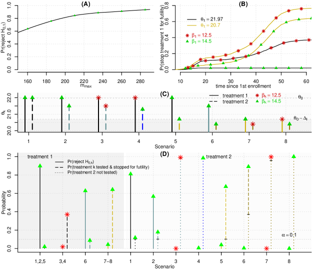
Figure 5: Operating characteristics of Bayesian de-intensification designs for a study with efficacy and toxicity co-primary endpoints. Panel A shows the power for treatment $k=1$ when $\theta_{1}=\theta_{0}$ and $\beta_{1}=\beta_{0}+2$ with maximum sample size $m_{\max}$ between $150$ and $300$ patients. Panel B shows the probability of stopping treatment $k=1$ for futility (either for inferior survival or low evidence of reduced toxicities) when $\theta_{1}=\theta_{0}$ (black curves) and $\beta_{1}=\beta_{0},\beta_{0}+2$ (red cross and green triangles) and when $\theta_{1}=\theta_{0}-\Delta=20.7$ (yellow curves) and $\beta_{1}=\beta_{0},\beta_{0}+2$ (red cross and green triangles) for a study with maximum sample size $m_{\max}=250$ patients. Panel C summarizes the 24-month RMSTs $(\theta_{k},\beta_{k}),k=1,2$ in each of the eight scenarios (x-axis) that we consider. The vertical bars (y-axis) indicate $\theta_{k}$, whereas green arrows ($\beta_{k}=14.5$) and red stars ($\beta_{k}=12.5$) on top of the vertical bars indicate toxicity parameters. Panel D shows, for both treatments, the power (solid bar), the probability of stopping treatment evaluation early for futility at IAs (dashed bars), and the probability that the 2nd treatment is not tested due to early termination of the study (dotted bars).

Panel B of Figure 5 shows the benefit of interim monitoring of efficacy and toxicity endpoints. The figure shows, for the first treatment, the cumulative probability of stopping the treatment for futility (y-axis), i.e. for inferiority or toxicity, by time $t$ since the first enrollment (x-axis) for four scenarios (scenarios 1, 3, 7 and 8: all combinations of $\theta_{1}=\theta_{0}-\Delta,\theta_{0}$ and $\beta_{1}=\beta_{0},\beta_{0}+2$). For instance, if the treatment is inferior with $\theta_{1}=\theta_{0}-\Delta=20.7$ but reduces toxicities ($\beta_{1}=\beta_{0}+2$), then 64% of all simulated de-intensification trials are stopped early for futility at IAs (scenario 8, golden curve with green triangle). In comparison, if the treatment fails to reduce toxicities ($\theta_{1}=20.7$ and $\beta_{1}=\beta_{0}$), then the treatment is stopped early for futility in 77% of the simulations (scenarios 7, golden curve with red stars).

Panel D of Figure 5 shows for both treatments the probability of rejecting $\mathcal{H}_{0,k}$ (power, solid vertical bars), and the probability that the study evaluates treatment $k$ and stops this arm early for futility (inferior survival or insufficient reduction of toxicities) at IAs (dashed vertical bars). As before the power for the 2nd treatment is defined as the probability that the study starts testing treatment 2 and rejects $\mathcal{H}_{0,2}$. For the 2nd treatment Panel D shows also the probability that the 2nd treatment is not tested due to early termination of the study (dotted vertical bars). If both treatments ($k=1,2$) extend the the RMST of the 1st AE by two months ($\beta_{1}=\beta_{2}=14.49$) compared to the SOC and have identical survival outcomes ($\theta_{1}=\theta_{2}=21.97$) the 1st and 2nd de-intensified treatment have $90\%$ and $82\%$ power (scenario 1). In comparison, with a moderate non-inferior treatment effect of $\theta_{k}=21.53$ in scenario 6 the power for the 1st treatment decreases to $63\%$.

Similar to the Bayesian design with efficacy primary endpoint of Section 2.1, scenarios 7 and 8 indicate the advantage of testing the 1st and 2nd treatment sequentially one after the other. If the first treatment is inferior, the second treatment $k=2$ is tested in 4% (scenario 7, $\beta_{1}=14.49$) or in less than $1\%$ (scenario 8, $\beta_{1}=12.49$) of all simulations. Scenario 4 shows one limitation of the design, here both treatments have non-inferior survival but only the 2nd treatment reduces toxicities, $\beta_{1}=12.49$ and $\beta_{2}=14.49$. In this case the study is terminated early without testing the second treatment in $98\%$ of all simulations.

5 Discussion

There has been a recent interest in developing de-intensified anti-cancer treatments with similar survival as the current SOC and reduced AEs. [7, 29] identified 12 de-intensification studies in oropharyngeal cancer that are currently ongoing or that recently reported results.

Compared to traditional superiority trials, which test superiority of experimental treatments compared to the SOC, demonstrating (i) similarity in survival between de-intensified treatments and the SOC, and (ii) reductions in AEs require large sample sizes. Investigators often select large NI margins to reduce the size of the study [43]. Recent results in oropharyngeal cancer showed that many de-intensification treatments fail to reduce toxicities and have inferior survival compared to the SOC [15, 28]. As discusses in [43], many of these studies (i) evaluate only survival or toxicity, (ii) do not have explicit futility early stopping rules for survival and toxicity endpoints, and (iii) tend to use conservative early stopping rules to avoid power reductions.

Motivated by a study at our institution, which tests two dose-reduced treatments, we proposed a Bayesian design for multi-arm de-intensification studies. The design tests non-inferior survival and toxicity reductions sequentially using a Bayesian non-parametric model. We proposed futility stopping rules to monitor both endpoints. The design parameters can be tuned to calibrated trade-offs between power and the probabilities of stopping arms early for inferior survival or insufficient evidence of toxicity reductions. In oropharynx cancer, where survival rates five years after IMRT+cisplatin treatment are $>90\%$, the number of observed OS and PFS events during the trial are typically small. Standard frequentist methods based on large-sample normal approximations can perform poorly in this setting and the Bayesian approach is an attractive alternative.

De-Intensified treatments in our design are tested one at the time, starting with the treatment with the highest dose-level. This controls the number of patients exposed to inferior treatments. As indicated in Section 4.3, one limitation of the Bayesian design is that it could stop the first non-inferior arm ($\theta_{1}>\theta_{0}+\Delta$) because of frequent toxicities and terminate the study, but the 2nd treatment may potentially reduce toxicities ($\beta_{2}>\beta_{0}$) with non-inferior survival ($\theta_{2}>\theta_{0}+\Delta$). The design can be modified, to account for this limitation, with a definition of the decision to terminate the study or not that distinguishes between negative results for arm 1 due to toxicities or due to PFS data.

We focused on non-controlled phase II de-intensification studies, but the design could be modified to include a concurrent control arm. If the SOC is associated with severe toxicities, it may be unethically to continue the assignment of patients to the SOC after the null hypothesis $\mathcal{H}_{0,1}$ has been rejected. In this case the 1st de-intensified treatment could be utilizes as the new control arm for testing the 2nd de-intensified experimental treatment.

References

- Ang et al. [2010] K. K. Ang, J. Harris, R. Wheeler, R. Weber, D. I. Rosenthal, P. F. Nguyen-Tan, W. H. Westra, C. H. Chung, R. C. Jordan, C. Lu, et al. Human papillomavirus and survival of patients with oropharyngeal cancer. New England Journal of Medicine, 363(1):24–35, 2010.
- Blackwelder [1982] W. C. Blackwelder. Proving the null hypothesis in clinical trials. Cont clinical trials, 3(4):345–353, 1982.
- Chan [2003] I. S. Chan. Proving non-inferiority or equivalence of two treatments with dichotomous endpoints using exact methods. Stat Med in Med Research, 12(1):37–58, 2003.
- Chen et al. [2011] M.-H. Chen, J. G. Ibrahim, P. Lam, A. Yu, and Y. Zhang. Bayesian design of noninferiority trials for medical devices using historical data. Biometrics, 67(3):1163–1170, 2011.
- D’Agostino et al. [2003] R. B. D’Agostino, J. M. Massaro, and L. M. Sullivan. Non-inferiority trials: design concepts and issues–the encounters of academic consultants in statistics. Stat Med, 22(2):169–186, 2003.
- Daimon [2008] T. Daimon. Bayesian sample size calculations for a non-inferiority test of two proportions in clinical trials. Cont clinical trials, 29(4):507–516, 2008.
- Elrefaey et al. [2014] S. Elrefaey, M. Massaro, S. Chiocca, F. Chiesa, and M. Ansarin. Hpv in oropharyngeal cancer: the basics to know in clinical practice. Acta Otorh Italica, 34(5):299, 2014.
- Farrington and Manning [1990] C. P. Farrington and G. Manning. Test statistics and sample size formulae for comparative binomial trials with null hypothesis of non-zero risk difference or non-unity relative risk. Stat Med, 9(12):1447–1454, 1990.
- Ferguson [1973] T. S. Ferguson. A bayesian analysis of some nonparametric problems. The annals of statistics, pages 209–230, 1973.
- Freidlin and Korn [2002] B. Freidlin and E. L. Korn. A comment on futility monitoring. Cont Clinical Trials, 23(4):355–366, 2002.
- Freidlin et al. [2007] B. Freidlin, E. L. Korn, S. L. George, and R. Gray. Randomized clinical trial design for assessing noninferiority when superiority is expected. JCO, 25(31):5019–5023, 2007.
- Freidlin et al. [2010] B. Freidlin, E. L. Korn, and R. Gray. A general inefficacy interim monitoring rule for randomized clinical trials. Clinical Trials, 7(3):197–208, 2010.
- Gamalo et al. [2011] M. A. Gamalo, R. Wu, and R. C. Tiwari. Bayesian approach to noninferiority trials for proportions. J of Biopharm Stat, 21(5):902–919, 2011.
- Gillison et al. [2000] M. L. Gillison, W. M. Koch, R. B. Capone, M. Spafford, W. H. Westra, L. Wu, M. L. Zahurak, R. W. Daniel, M. Viglione, D. E. Symer, et al. Evidence for a causal association between human papillomavirus and a subset of head and neck cancers. JNCI, 92(9):709–720, 2000.
- Gillison et al. [2019] M. L. Gillison, A. M. Trotti, J. Harris, A. Eisbruch, P. M. Harari, D. J. Adelstein, E. M. Sturgis, B. Burtness, J. A. Ridge, J. Ringash, et al. Radiotherapy plus cetuximab or cisplatin in human papillomavirus-positive oropharyngeal cancer (nrg oncology rtog 1016): a randomised, multicentre, non-inferiority trial. The Lancet, 393(10166):40–50, 2019.
- Hjort et al. [1990] N. L. Hjort et al. Nonparametric bayes estimators based on beta processes in models for life history data. The Annals of Statistics, 18(3):1259–1294, 1990.
- Holmgren [1999] E. B. Holmgren. Establishing equivalence by showing that a specified percentage of the effect of the active control over placebo is maintained. J of Biopharm Stat, 9(4):651–659, 1999.
- Hurvitz et al. [2018] S. A. Hurvitz, M. Martin, W. F. Symmans, K. H. Jung, C.-S. Huang, A. M. Thompson, N. Harbeck, V. Valero, D. Stroyakovskiy, H. Wildiers, et al. Neoadjuvant trastuzumab, pertuzumab, and chemotherapy versus trastuzumab emtansine plus pertuzumab in patients with her2-positive breast cancer (kristine): a randomised, open-label, multicentre, phase 3 trial. Lancet Onc, 19(1):115–126, 2018.
- [19] I. Bormann. Digitizeit. URL https://www.digitizeit.de.
- Jennison and Turnbull [1989] C. Jennison and B. W. Turnbull. Interim analyses: the repeated confidence interval approach. JRSS-B, 51(3):305–334, 1989.
- Joshua Chen and Chen [2012] Y. Joshua Chen and C. Chen. Testing superiority at interim analyses in a non-inferiority trial. Stat Med, 31(15):1531–1542, 2012.
- Korn and Freidlin [2017] E. Korn and B. Freidlin. Interim monitoring for non-inferiority trials: minimizing patient exposure to inferior therapies. Ann of Oncology, 29(3):573–577, 2017.
- Lachin [2009] J. M. Lachin. Futility interim monitoring with control of type i and ii error probabilities using the interim z-value or confidence limit. Clinical Trials, 6(6):565–573, 2009.
- Laster et al. [2006] L. Laster, M. F. Johnson, and M. Kotler. Non-inferiority trials. Stat Med, 25(7):1115–1130, 2006.
- Llombart-Cussac et al. [2017] A. Llombart-Cussac, J. Cortés, L. Paré, P. Galván, B. Bermejo, N. Martínez, M. Vidal, S. Pernas, R. López, M. Muñoz, et al. Her2-enriched subtype as a predictor of pathological complete response following trastuzumab and lapatinib without chemotherapy in early-stage her2-positive breast cancer (pamela): an open-label, single-group, multicentre, phase 2 trial. Lancet Onc, 18(4):545–554, 2017.
- Marur et al. [2017] S. Marur, S. Li, A. J. Cmelak, M. L. Gillison, W. J. Zhao, R. L. Ferris, W. H. Westra, J. Gilbert, J. E. Bauman, L. I. Wagner, et al. E1308: phase ii trial of induction chemotherapy followed by reduced-dose radiation and weekly cetuximab in patients with hpv-associated resectable squamous cell carcinoma of the oropharynx. JCO, 35(5):490, 2017.
- Mathew and Brufsky [2017] A. Mathew and A. Brufsky. Less is more? de-intensification of therapy for early-stage her2-positive breast cancer. Lancet Onc, 18(4):428–429, 2017.
- Mehanna et al. [2019] H. Mehanna, M. Robinson, A. Hartley, A. Kong, B. Foran, T. Fulton-Lieuw, M. Dalby, P. Mistry, M. Sen, L. O’Toole, et al. Radiotherapy plus cisplatin or cetuximab in low-risk human papillomavirus-positive oropharyngeal cancer: an open-label randomized controlled phase 3 trial. The Lancet, 393(10166):51–60, 2019.
- Mirghani and Blanchard [2018] H. Mirghani and P. Blanchard. Treatment de-escalation for hpv-driven oropharyngeal cancer: Where do we stand? Clinical and translational radiation oncology, 8:4–11, 2018.
- Munker et al. [2001] R. Munker, L. Purmale, Ü. Aydemir, M. Reitmeier, H. Pohlmann, H. Schorer, and R. Hartenstein. Advanced head and neck cancer: long-term results of chemo-radiotherapy, complications and induction of second malignancies. Oncology Research and Treatment, 24(6):553–558, 2001.
- O’Brien and Fleming [1979] P. C. O’Brien and T. R. Fleming. A multiple testing procedure for clinical trials. Biometrics, pages 549–556, 1979.
- Osman and Ghosh [2011] M. Osman and S. K. Ghosh. Semiparametric bayesian testing procedure for noninferiority trials with binary endpoints. J of Biopharm Stat, 21(5):920–937, 2011.
- Pocock [1977] S. J. Pocock. Group sequential methods in the design and analysis of clinical trials. Biometrika, 64(2):191–199, 1977.
- Reboussin et al. [2000] D. M. Reboussin, D. L. DeMets, K. Kim, and K. G. Lan. Computations for group sequential boundaries using the lan-demets spending function method. Controlled clinical trials, 21(3):190–207, 2000.
- Rothmann et al. [2003] M. Rothmann, N. Li, G. Chen, G. Y. Chi, R. Temple, and H.-H. Tsou. Design and analysis of non-inferiority mortality trials in oncology. Stat Med, 22(2):239–264, 2003.
- Schmidli et al. [2013] H. Schmidli, S. Wandel, and B. Neuenschwander. The network meta-analytic-predictive approach to non-inferiority trials. Stat Med in Med Research, 22(2):219–240, 2013.
- Seiwert et al. [2019a] T. Seiwert, C. Foster, E. Blair, T. Karrison, N. Agrawal, J. Melotek, L. Portugal, R. Brisson, A. Dekker, S. Kochanny, et al. Optima: a phase ii dose and volume de-escalation trial for human papillomavirus-positive oropharyngeal cancer. Annals of Oncology, 30(2):297–302, 2019a.
- Seiwert et al. [2019b] T. Seiwert, C. Foster, E. Blair, T. Karrison, N. Agrawal, J. Melotek, L. Portugal, R. Brisson, A. Dekker, S. Kochanny, et al. Optima: a phase ii dose and volume de-escalation trial for human papillomavirus-positive oropharyngeal cancer. Annals of Oncology, 30(2):297–302, 2019b.
- Semenza [2008] G. L. Semenza. A new weapon for attacking tumor blood vessels. New England Journal of Medicine, 358(19):2066–2067, 2008.
- Simon [1999] R. Simon. Bayesian design and analysis of active control clinical trials. Biometrics, 55(2):484–487, 1999.
- Snapinn [2004] S. M. Snapinn. Alternatives for discounting in the analysis of noninferiority trials. J of Biopharm Stat, 14(2):263–273, 2004.
- Tu [1998] D. Tu. On the use of the ratio or the odds ratio of cure rates in therapeutic equivalence clinical trials with binary endpoints. J of Biopharm Stat, 8(2):263–282, 1998.
- Ventz et al. [2019] S. Ventz, L. Trippa, and J. D. Schoenfeld. Lessons learned from de-escalation trials in favorable risk hpv-associated schn cancer. Clinical Cancer Research, page (in press), 2019.
- Walker and Muliere [1997] S. Walker and P. Muliere. Beta-stacy processes and a generalization of the pólya-urn scheme. The Annals of Statistics, pages 1762–1780, 1997.
- Wellek [2005] S. Wellek. Statistical methods for the analysis of two-arm non-inferiority trials with binary outcomes. Biom Journal, 47(1):48–61, 2005.
- Williamson [2007] P. P. Williamson. Bayesian equivalence testing for binomial random variables. Journal of Statistical Computation and Simulation, 77(9):739–755, 2007.
- Zhao et al. [2016] L. Zhao, B. Claggett, L. Tian, H. Uno, M. A. Pfeffer, S. D. Solomon, L. Trippa, and L. Wei. On the restricted mean survival time curve in survival analysis. Biometrics, 72(1):215–221, 2016.