Surface Brightness Profile of Halos out to $320$ kpc in HETDEX

Abstract

We present the median-stacked surface brightness profile of 968 spectroscopically selected emitting galaxies (LAEs) at redshifts $1.9<z<3.5$ in the early data of the Hobby-Eberly Telescope Dark Energy Experiment (HETDEX). The selected LAEs are high-confidence detections with large signal-to-noise ratios observed with good seeing conditions (point-spread-function full-width-at-half-maximum $<1.4^{\prime\prime}$), excluding active galactic nuclei (AGN). The luminosities of the LAEs are $10^{42.4}-10^{43}\,\mathrm{erg}\,\mathrm{s}^{-1}$. We detect faint emission in the median-stacked radial profiles at the level of $(3.6\pm 1.3)\times 10^{-20}\,\mathrm{erg}\,\mathrm{s}^{-1}\,\mathrm{cm}^{-2}\,\mathrm{arcsec}^{-2}$ from the surrounding halos out to $r\simeq 160$ kpc (physical). The shape of the median-stacked radial profile is consistent at $r<80\,\mathrm{kpc}$ with that of much fainter LAEs at $3<z<4$ observed with the Multi Unit Spectroscopic Explorer (MUSE), indicating that the median-stacked Lyman-$\alpha$ profiles have similar shapes at redshifts $2<z<4$ and across a factor of $10$ in luminosity. While we agree with the results from the MUSE sample at $r<80\,\mathrm{kpc}$, we extend the profile over a factor of two in radius. At $r>80\,\mathrm{kpc}$, our profile is flatter than the MUSE model. The measured profile agrees at most radii with that of galaxies in the Byrohl et al. (2021) cosmological radiative transfer simulation at $z=3$. This suggests that the surface brightness of a Lyman-$\alpha$ halo at $r\lesssim 100$ kpc is dominated by resonant scattering of photons from star-forming regions in the central galaxy, whereas at $r>100$ kpc it is dominated by photons from galaxies in surrounding dark matter halos.

1 Introduction

Large emission regions with sizes of tens to hundreds of kpc were first found around high-redshift radio galaxies (McCarthy et al., 1987; van Ojik et al., 1997; Overzier et al., 2001; Reuland et al., 2003). Later, they were observed around quasars (Weidinger et al., 2004, 2005; Christensen et al., 2006; Smith et al., 2009; Goto et al., 2009; Cantalupo et al., 2014; Martin et al., 2014b, a; Hennawi et al., 2015; Arrigoni Battaia et al., 2016; Borisova et al., 2016; Cai et al., 2018; Arrigoni Battaia et al., 2019a; Kikuta et al., 2019; Zhang et al., 2020), star-forming galaxies (Smith & Jarvis, 2007; Smith et al., 2008; Shibuya et al., 2018), and in galaxy-overdense regions (Steidel et al., 2000; Matsuda et al., 2004, 2011; Yang et al., 2010; Cai et al., 2017). Measurements of the cross-correlation of intensity with quasar (Croft et al., 2016, 2018) or LAE positions (Kakuma et al., 2021; Kikuchihara et al., 2021) revealed emission on even larger scales. Most individual high-redshift star-forming galaxies such as emitting galaxies (LAEs) and Lyman-break galaxies (LBGs) are surrounded by smaller, $1-10$ kpc-size halos (Hayashino et al., 2004; Swinbank et al., 2007; Rauch et al., 2008; Ouchi et al., 2009; Wisotzki et al., 2016; Patrício et al., 2016; Smit et al., 2017; Leclercq et al., 2017; Erb et al., 2018; Claeyssens et al., 2019, 2022). Kusakabe et al. (2022) detected halos with sizes between $10$ and $50\,\mathrm{kpc}$ in 17 out of 21 continuum-selected galaxies. While Bond et al. (2010), Feldmeier et al. (2013), and Jiang et al. (2013) report a lack of evidence for spatially extended emission around LAEs and LBGs, the ubiquitous presence of extended halos around high-redshift star-forming galaxies has been confirmed by stacking analyses (Møller & Warren, 1998; Steidel et al., 2011; Matsuda et al., 2012; Momose et al., 2014, 2016; Xue et al., 2017; Wisotzki et al., 2018; Wu et al., 2020; Huang et al., 2021). The Multi Unit Spectroscopic Explorer (MUSE, Bacon et al. 2010) on the Very Large Telescope (VLT) has revolutionized the subject by using up to $31$ hour exposures to explore halos. By co-adding a sample of $270$ LAEs at $3<z<6$ in a $2\,\mathrm{arcmin}^{2}$ section of sky, Wisotzki et al. (2018) found that emission can be traced out to several arcseconds from the source centers, so that nearly all the sky is covered by emission around high-redshift galaxies in projection.

The size of the halos around LAEs depends on their physical properties such as the ultraviolet (UV) and luminosities and the size of the UV-emitting region (Wisotzki et al., 2016; Xue et al., 2017; Momose et al., 2016; Leclercq et al., 2017). While halos are more compact in nearby galaxies than in high-redshift galaxies (e.g. Hayes et al., 2005; Östlin et al., 2009; Hayes et al., 2013, 2014; Leclercq et al., 2017; Rasekh et al., 2021), no significant redshift evolution of halos around LAEs within $2<z<6$ has been detected (Momose et al., 2014; Leclercq et al., 2017; Kikuchihara et al., 2021). In contrast, observed halo profiles of quasars are shown to increase from $z\sim 2$ to $z\sim 3$ and remain constant from $z\sim 3$ to $z\sim 6$ (Arrigoni Battaia et al., 2016, 2019a; Farina et al., 2019; Cai et al., 2019; O’Sullivan et al., 2020; Fossati et al., 2021).

There are various sources of photons that may contribute to the extended emission. One substantial source of photons is the local recombination of hydrogen atoms ionized by photons from young, massive stars in star-forming galaxies or from active galactic nuclei (AGN; Dijkstra, 2019). Due to their resonant nature, photons are scattered by neutral hydrogen atoms in the circumgalactic medium (CGM) and the intergalactic medium (IGM). photons can also be created by collisional excitation, such as when dense gas flows into a galaxy (called “gravitational cooling” Haiman et al., 2000; Fardal et al., 2001; Faucher-Giguère et al., 2010), and by fluorescence of hydrogen gas ionized by photons from more distant AGN or star-forming regions (called the “UV background”; Gould & Weinberg, 1996; Cantalupo et al., 2005; Kollmeier et al., 2010; Mas-Ribas & Dijkstra, 2016). Satellite galaxies can also contribute to the extended emission (Mas-Ribas et al., 2017).

In order to constrain the contributions of emission sources and mechanisms, it is necessary to model emission and its radiative transfer realistically. One method to model radiative transfer in halos is a perturbative approach (e.g. Kakiichi & Dijkstra, 2018). Another way uses hydrodynamical simulations that resolve the gas around galaxies, which can be post-processed with a Monte-Carlo radiative transfer calculation to predict the shape of emission around galaxies (e.g. Lake et al., 2015; Mitchell et al., 2021; Kimock et al., 2021). Most of these models simulate small numbers of galaxies, while Zheng et al. (2011), Gronke & Bird (2017) and Byrohl et al. (2021) calculate radiative transfer in cosmological hydrodynamical simulations and offer predictions for large samples of galaxies. While being a promising tool, hydrodynamical simulations of galaxy formation in cosmological volumes with sub-kpc resolutions (e.g. Nelson et al., 2020) possibly suffer from convergence issues both in the physical gas state (e.g. van de Voort et al., 2019) and radiative transfer (e.g. Camps et al., 2021).

Comparisons of predictions with measurements draw different conclusions. While Steidel et al. (2011), Gronke & Bird (2017), and Byrohl et al. (2021) find that most of the extended emission can be explained by scattering of photons from the central galaxy or nearby galaxies, Lake et al. (2015) stressed the importance of cooling radiation in producing halos when they compared their simulation with observations from Momose et al. (2014). Mitchell et al. (2021) report that satellite galaxies are the predominant source of photons at $10-40\,\mathrm{kpc}$, while cooling radiation also plays a relevant role.

Since the dominant origin of the halo photons depends on, among other things, the distance to the galaxies (Mitchell et al., 2021; Byrohl et al., 2021), observations of profiles out to larger distances will be helpful. An ideal data set for this is provided by the Hobby-Eberly Telescope Dark Energy Experiment (HETDEX; Hill et al., 2008; Gebhardt et al., 2021; Hill et al., 2021), which is designed to detect more than one million LAEs at redshifts $1.9<z<3.5$ in a $10.9\,\mathrm{Gpc}^{3}$ volume to measure their clustering and thereby constrain cosmological parameters. HETDEX detects emission lines by simultaneously acquiring tens of thousands of spectra without any pre-selecting of targets. In this work, we measure the median radial surface brightness profile of 968 LAEs at $1.9<z<3.5$ using the HETDEX data. We take advantage of the wide field of view of HETDEX and expand the measurement out to $320\,\mathrm{kpc}$ from the LAE centers.

This paper is structured as follows. Section 2 describes the data, the data processing, and the definition of the LAE sample. Section 3 presents the method to obtain the median radial surface brightness profile of the LAEs and how we account for systematic errors. Section 4 reports the results and shows that simple stacking of the surface brightness profiles reproduces the rescaled best-fit model of stacked halos at higher redshift ($3<z<4$) at $r<80\,\mathrm{kpc}$ from Wisotzki et al. (2018). We quantify the effect of possible AGN contamination in the LAE sample by stacking sources with broad lines and high luminosities. In Section 5, we compare our results with theoretical predictions from a radiative transfer simulation by Byrohl et al. (2021) and from a perturbative approach by Kakiichi & Dijkstra (2018). We conclude in Section 6.

We assume a flat $\Lambda$ cold dark matter ($\Lambda$CDM) cosmology consistent with the latest results from the Planck mission: $H_{0}=67.37\,\mathrm{km}\,\mathrm{s}^{-1}\,\mathrm{Mpc}^{-1}$ and $\Omega_{\mathrm{m},0}=0.3147$ (Planck Collaboration et al., 2020). All distances are in units of physical kpc/Mpc unless noted otherwise.

2 Data and Galaxy Sample

2.1 Data and Data Processing

We use spectra from the internal data release 2.1.3 (DR 2.1.3) of HETDEX, which were obtained with the Visible Integral-field Replicable Unit Spectrograph (VIRUS) on the $10\,\mathrm{m}$ Hobby-Eberly Telescope (HET, Ramsey et al. 1994; Hill et al. 2021). VIRUS consists of up to 78 integral-field unit fiber arrays (IFUs), each of which contains 448 $1.5^{\prime\prime}$-diameter fibers and spans $51^{\prime\prime}\times 51^{\prime\prime}$ on the sky. The fibers from each IFU are fed to a low-resolution ($R=800$) spectrograph unit containing two spectral channels, which covers the wavelengths between $3500\,\textup{\AA}$ and $5500\,\textup{\AA}$. Each spectral channel has a CCD detector with two amplifiers; the spectra from the 448 fibers of each IFU are effectively split over four amplifiers. The IFUs with $\sim$ 35k total fibers are distributed throughout the $18^{\prime}$ diameter of the telescope’s field of view. Each HETDEX observation includes three 6-minute exposures, which are dithered to fill in gaps between the fibers. The IFUs are arrayed on a grid with $100^{\prime\prime}$ spacing. The gaps between the IFUs remain, so that the filling factor of one observation is $\sim 1/4.6$. Details of the upgraded HET and the VIRUS instrument can be found in Hill et al. (2021).

The data processing pipeline is described in Gebhardt et al. (2021). A crucial aspect for detecting low surface brightness emission is the sky subtraction. HETDEX applies two separate approaches to sky subtraction, one using a local sky determined from a single amplifier (112 fibers spanning $\sim 0.2\,\mathrm{arcmin}^{2}$), and a full-frame sky determined from the full array of IFUs (over 30k fibers).

For the local sky subtraction, we identify continuum sources by extracting a continuum estimate for each of the 112 fibers on a given amplifier using a wavelength range of $4100-5100\,\textup{\AA}$. We flag fibers with a $>3\sigma$ detection of continuum (using a biweight scale as $\sigma$; Beers et al., 1990) as continuum fibers. We further flag the two adjacent fibers in the spectroscopic image to each continuum fiber. This typically removes about $15\%$ of the fibers. Of the remaining fibers, we apply a further cut of $10\%$ of the fibers with the highest counts in the continuum region. The biweight location, which is a robust estimate of the central location of a distribution (Beers et al., 1990), of the remaining approximately $75\%$ of the fibers determines the local sky spectrum. There is residual low-level background that is due to a combination of dark current, scattered light, mismatch of the fiber profile, and illumination differences for the specific exposure. After removing the identified continuum sources, we smooth the spectroscopic image with a two-dimensional biweight filter that is six fibers by $700\,\textup{\AA}$ across in order to estimate and remove the broad-scale residual background (“background light correction”). This procedure is highly effective at removing the residual background at the expense of removing some continuum of faint sources. While this local sky subtraction is robust, extended emission that covers a significant fraction of the small area of an amplifier can be mistaken as sky emission and thus removed from the signal.

As an alternative, HETDEX provides a full-frame sky subtraction. This procedure uses over 30k fibers, which provides significant improvement for objects that dominate an amplifier. Continuum sources are identified in the same manner as the local sky estimate. The disadvantage of this procedure is that the amplifiers have their individual differences which need to be addressed. These include differences in the illumination of the primary mirror on the IFUs across the $20^{\prime}$ field, the wavelength solution, and the instrumental dispersion.

There are two components to the amplifier-to-amplifier normalization for the full-frame sky spectrum. The first component is the instrumental throughput difference that we measure from the twilight frames. The second is due to the different illumination patterns of the primary as the HET tracks a specific field, leading to illumination differences of the IFUs. We use the relative residual flux in the sky-subtracted images to determine the relative normalizations due to illumination. Because there a broad wavelength dependence, we use a low-order term to adjust the normalization for each amplifier coming from $4$ wavelength regions averaged over $500\,\textup{\AA}$ regions. The scalings range from $0.9$ to $1.1$, and we use deviations beyond this range as a flag for data that potentially has to be removed due detector controller issues. The wavelength dependence is small, generally under $1\%$. Since the local sky subtraction uses one sky spectrum for each amplifier, the illumination differences are irrelevant.

The other important aspect is due to small changes in the wavelength solution. We use the full-frame sky wavelength solution to adjust the local values. During the full-frame sky subtraction, we allow each amplifier to fit for a wavelength offset and a dispersion term. The offsets are generally small (less than $0.2\,\textup{\AA}$), but the dispersion term can be more important. We think that the dispersion term is caused by differential breathing modes in the spectrograph due to temperature changes. For the majority of amplifiers, the sky-subtracted frames from the full frame and local sky look very similar. There are a few where the dispersion term does not adequately capture the changes in the wavelength solution, causing small residuals correlated with bright sky lines. The background residual counts within a given amplifier still need to be removed, which will subtract some light from the faintest sources. We are confident that, while there remains some uncertainty in the background estimate, the line flux relative to the continuum is unaffected.

One aspect we do not account for are changes in instrumental resolution across spectrographs. While we have built these to have as uniform resolving power as possible, there are differences. In particular, the resolution can change across the amplifier, where fibers at the edge of spectrographs have larger instrumental dispersion. The local sky subtraction naturally deals with the variation from spectrograph to spectrograph, whereas the full-frame does not. The variation within a spectrograph is equally a problem in both sky subtraction procedures. We do not address these differences at this point. The effect is small, and only noticeable at some of the edges of spectrographs. To compensate for these issues, our noise model takes into account the larger residuals and increases the noise at those locations. The number of fibers affected by this increased noise is under 5%.

The full-frame sky subtraction over the large field of view of VIRUS offers an advantage for extended objects over the local sky subtraction and over instruments such as MUSE, which has a smaller field of view with which to measure the sky spectrum. We therefore adopt the full-frame sky subtraction.

2.2 LAE Sample

We draw our sample of LAEs from the line emission catalog from the HETDEX internal data release 2 (specifically v2.1.3) to be published in Mentuch Cooper et al., in preparation, which contains approximately 300k LAEs. For each detected line, the catalog provides the coordinates of the centroid, the central wavelength, the line width, the line flux, the signal-to-noise ratio ($S/N$), and the probability of the feature being a line. This probability is computed by the HETDEX Emission Line eXplorer (ELiXer) (Davis et al., in preparation), which uses multiple techniques including a Bayesian Lyman-$\alpha$-vs-[O II] $\lambda\,3727$ discrimination (Leung et al., 2017; Farrow et al., 2021). To minimize contamination of nearby objects and artifacts, the ELiXer probability $P(\mathrm{Ly}\alpha)$ of every line in our sample must be larger than $0.9$ (the minimum $P(\mathrm{Ly}\alpha)/P($[O II]$)$ is 9).

We require that the lines have $S/N\geq 6.5$ to minimize false positive detections. The minimum throughput at $4540\,\textup{\AA}$ of an observation must be $>0.08$ for HETDEX to include its line detections in the catalog. In this work, we only include LAEs in observations with throughput $>0.13$ and good seeing (PSF full-width-at-half-maximum (FWHM) $<1.4^{\prime\prime}$) to resolve the halos. Furthermore, we only use observations that were taken in 2019 and later, as earlier data had more detector artifacts and often larger sky emission residuals.

After visually inspecting the remaining sources and excluding non-LAEs, our sample consists of 1491 high-confidence high-redshift emitting objects, which are detected in 150 observations.

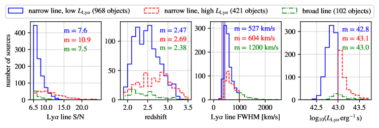
Figure 1: Distributions and median values (m) of several properties of the sources in the three samples: NLLL sources are shown in solid blue, NLHL sources are shown in dashed red, and BL sources are shown in dot-dashed green. The first panel presents the $S/N$ distributions for $S/N\geq 6.5$. the second panel displays the redshift distributions. The third panel shows the Lyman-$\alpha$-line FWHM. The purple shaded area shows the instrumental resolution over the redshift range of the instrument ($5.6\textup{\AA}$; Hill et al., 2021). The narrow-line and broad-line samples are separated at $\mathrm{FWHM}_{\mathrm{Ly}\alpha}=1000\,\mathrm{km}\,\mathrm{s}^{-1}$. The fourth panel shows the luminosity. Because of the high-$S/N$ requirement, the sources have luminosities $>10^{42.4}\,\mathrm{erg}\,\mathrm{s}^{-1}$. The low- and high-luminosity samples are divided at $L_{\mathrm{Ly}\alpha}=10^{43}\,\mathrm{erg}\,\mathrm{s}^{-1}$.

This initial sample contains AGN. Since we are interested in the halos of LAEs without an AGN, we divide the sample into three subgroups. The first criterion is the line width: galaxies with a line $\mathrm{FWHM}_{\mathrm{Ly}\alpha}\geq 1000\,\mathrm{km}\,\mathrm{s}^{-1}$ are placed into the broad-line sample (BL, 102 objects). The remaining sources are separated by their luminosity: galaxies with a luminosity $L_{\mathrm{Ly}\alpha}\geq 10^{43}\,\mathrm{erg}\,\mathrm{s}^{-1}$ constitute the narrow-line, high-luminosity sample (NLHL, 421 objects), whereas galaxies with $L_{\mathrm{Ly}\alpha}<10^{43}\,\mathrm{erg}\,\mathrm{s}^{-1}$ constitute the narrow-line, low-luminosity (NLLL) sample (968 objects). We use the NLLL subset as our final LAE sample. The luminosity threshold represents the luminosity at which narrow-band selected LAEs start to be dominated by AGN (Spinoso et al., 2020). Zhang et al. (2021) find that the AGN fraction at $2.0<z<3.5$ at $L_{\mathrm{Ly}\alpha}<10^{43}\,\mathrm{erg}\,\mathrm{s}^{-1}$ is $<0.05$; hence this is a conservative threshold. In this fashion we remove most AGN from the NLLL/LAE sample. We compare the median radial profile of the LAE sample to those of the other two samples to study the impact of potential AGN contamination.

Figure 1 shows the distributions of $S/N$, redshift, Lyman-$\alpha$-line FWHM, and luminosities of the NLLL (blue), the NLHL (red), and the BL (green) samples. Figure 2 displays the median spectrum of the NLLL/LAEs in the rest frame without continuum subtraction. We interpolate the spectra of the closest fiber to each LAE on a rest-frame wavelength grid with a bin size of $0.4\,\textup{\AA}$. Then we take the median of the individual LAE spectra.

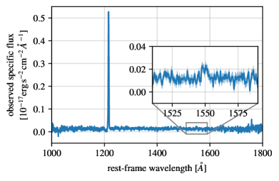
Figure 2: Median spectrum of the 968 LAEs in the NLLL sample in the rest frame. We use the original, not continuum-subtracted, spectrum of the fiber closest to each LAE. The observed specific flux is interpolated on a regular rest-frame wavelength grid with $0.4\,\textup{\AA}$ binning to obtain the median spectrum. The inset shows the C IV emission line ($\mathrm{EW}_{\mathrm{C}\textsc{iv}}=4.0\pm 0.7\,\textup{\AA}$).

The median spectrum possesses continuum, a prominent line ($1216\,\textup{\AA}$), and a faint C IV line ($1550\,\textup{\AA}$). The large observed equivalent width ($\mathrm{EW}_{\mathrm{Ly}\alpha}=96\pm 3\,\textup{\AA}$) indicates that the LAE sample mainly consists of emitting galaxies, rather than low-$z$ [O II] galaxies (Ciardullo et al., 2013; Santos et al., 2020). The strength of C IV emission ($\mathrm{EW}_{\mathrm{C}\textsc{iv}}=4.0\pm 0.7\,\textup{\AA}$) is consistent with predictions for star-forming galaxies (Nakajima et al., 2018). It is also within the range reported by Feltre et al. (2020), who studied the mean rest-frame UV spectra of LAEs at $2.9<z<4.6$ using MUSE. Our NLHL sample has a similar equivalent width ($\mathrm{EW}_{\mathrm{Ly}\alpha}=94\pm 3\,\textup{\AA}$) and C IV emission ($\mathrm{EW}_{\mathrm{C}\textsc{iv}}=3.4\pm 0.7\,\textup{\AA}$). Our BL sample has a similar equivalent width ($\mathrm{EW}_{\mathrm{Ly}\alpha}=103\pm 7\,\textup{\AA}$), but larger C IV emission ($\mathrm{EW}_{\mathrm{C}\textsc{iv}}=5.5\pm 1.5\,\textup{\AA}$), as expected for a larger fraction of AGN in the sample. The N V ($1239\,\textup{\AA}$ and $1243\,\textup{\AA}$) and Si IV ($1394\,\textup{\AA}$ and $1403\,\textup{\AA}$) emission lines are not detected in median spectra of the NLLL, NLHL, or BL samples. The median spectra of the NLLL and NLHL samples have a He II ($1640\,\textup{\AA}$) equivalent width of $2.2\pm 0.6\,\textup{\AA}$, which is consistent with that of bright ($L_{\mathrm{Ly}\alpha}>10^{42.05}\,\mathrm{erg}\,\mathrm{s}^{-1}$) LAEs reported by Feltre et al. (2020).

2.3 Masking and Continuum Subtraction

We mask the wavelength regions around bright sky lines to avoid the largest sky emission residuals.

To isolate the emission, we remove continuum emission of the LAEs from the spectra. In each fiber, we subtract the median flux within $40\,\textup{\AA}$ of the line center, but excluding the central $5\,\sigma_{\mathrm{Ly}\alpha}$, where $\sigma_{\mathrm{Ly}\alpha}$ is a Gaussian $\sigma$ from the fit to the emission line. Subtracting only the continuum on the red side of the line or changing the excluded central window from $5\sigma_{\mathrm{Ly}\alpha}$ to $7\sigma_{\mathrm{Ly}\alpha}$ does not affect our results. We subtract the continuum emission of all fibers instead of masking those with high continuum emission for multiple reasons. Most importantly, the resulting surface brightness profiles have insignificant differences because the continuum subtraction successfully removes the continuum flux from projected neighbors. It is also difficult to mask continuum sources completely because of the large PSF of VIRUS. In the masking scheme, many fibers in the core of our LAE sample were masked. Finally, the continuum subtraction removes the systematic effect from an incorrect background subtraction, which can add a constant or smooth wavelength-dependent flux to each spectrum.

3 Detection of Lyman-$\alpha$ halos

3.1 Extraction of Lyman-$\alpha$ Surface Brightness

We integrate the flux density over the wavelengths around the line of each LAE to obtain a surface brightness for each fibers that is located within $320\,\mathrm{kpc}$ of the LAE (typically 1100 fibers). The width of this integration window is different for each LAE and is chosen to be three times the $\sigma_{\mathrm{Ly}\alpha}$ of the Gaussian fit to the LAE’s emission line. The integration window widths range from $5\,\textup{\AA}$ to $18\,\textup{\AA}$ (NLLL sample) in the observed reference frame, with a median (mean) of $10\,\textup{\AA}$ ($12\,\textup{\AA}$). To investigate the influence of the variable width on the radial profile measurement, the measurement was repeated with a fixed width of $\Delta\lambda=11\,\textup{\AA}$; the results are consistent with one another. We choose the variable-width approach because the results have slightly higher S/N.

The result of this preparation is a set of surface brightness values as a function of angular separation from the centroid of each LAE. We translate this angular distance to a physical distance assuming our fiducial cosmology and sort the fibers around each LAE by their distance from it.

3.2 Stacking

We take the median surface brightness of all fibers around all LAEs in radial bins. The bin edges are at $[5,10,15,20,25,30,40,60,80,160,320]\,\mathrm{kpc}$. In each bin we gather all fibers whose distance from the fiber center to their corresponding LAE lies within this range. We do not normalize the surface brightness of the fibers around each LAE in order to retain physical units. We take the median surface brightness of these fibers and use a bootstrap algorithm to determine the uncertainty. Each bin contains fibers from at least $55\%$ of LAEs in the NLLL sample, and at $r>10\,\mathrm{kpc}$, more than $96\%$ of the LAEs contribute to each bin.

3.3 Estimating Systematic Uncertainty

We explore the systematic uncertainty in two steps. The first part addresses the median surface brightness that would be interpreted as extended emission in random locations on the sky rather than centered on an LAE, which we refer to as the background surface brightness. One total value is used for this quantity, which is the sum of contributions from emission in the target redshift, other redshifted emission lines, continuum emission from stars and nearby galaxies, and sky emission residuals. To measure this background surface brightness, we repeat our surface brightness measurements at random locations. Specifically, for each LAE we randomly draw a fiber within the same observation and choose a random location within $1^{\prime\prime}$ of this fiber as the centroid. To avoid the possibility of any of the LAE’s halo affecting our experiment, we require that this new position be further than $2^{\prime}$ from the original LAE. These random locations may coincide with foreground objects. This is intentional because we probe the halos out to $>30^{\prime\prime}$, which can include foreground objects. It is therefore appropriate not to exclude these from the random sample. We then integrate the flux of the fibers within $20^{\prime\prime}$ of this location over the same wavelengths used for the integration of the real LAE. For each LAE, we generate three of these random measurements, producing a data set for comparison that has the same distribution of wavelengths and widths of integration windows as the LAE, but is centered on random, but not necessarily empty, sky positions. Because we prepare the spectra identically to those around LAEs, this background estimate accounts for potential systematic effects introduced by the continuum subtraction.

We use the median of our random position measurements to estimate the background surface brightness and a bootstrap algorithm to estimate the uncertainty. We find $(4.0\pm 0.4)\times 10^{-20}\,\mathrm{erg}\,\mathrm{s}^{-1}\,\mathrm{cm}^{-2}\,\mathrm{arcsec}^{-2}$ for the NLLL sample. The non-zero background does not contradict the efficacy of the full-frame sky subtraction. It can be caused for example by the complicated, asymmetric shape of the pixel flux distribution, non-flat fiber spectra, and differences in averaging estimators.

Having considered systematic uncertainties derived on larger volumes, we now address systematic errors associated with proximity of the LAEs. This second step largely follows the procedure of Wisotzki et al. (2018). For each LAE we repeat the surface brightness extraction, but shift the central wavelength in increments of $10\,\textup{\AA}$ from the observed wavelength, where the minimum offset is $20\,\textup{\AA}$ and the maximum offset is $210\,\textup{\AA}$. This produces 40 sets of Lyman-$\alpha$-free pseudo-narrow-band images for each LAE, which we then combine to make 40 Lyman-$\alpha$-free stacks, each separated by $\Delta\lambda$. Their standard deviation is then defined as the empirical uncertainty of the stack of LAEs. The median ratio of these empirical errors to the statistical error using the bootstrap algorithm is $1.5$. We adopt the larger of the two error estimates as the uncertainty of the median surface brightness in each bin. The median of the wavelength-shifted profiles is consistent with the background at $r>50\,\mathrm{kpc}$.

We subtract the background surface brightness to find the median surface brightness profile around our LAE sample. Since the random sample depends on the sample of sources, the BL, NLHL, and NLLL samples each have one background surface brightness. The uncertainty of the background estimate is included in the uncertainty of the final surface brightness profile via Gaussian error propagation.

We can compare the reported errors to the propagation of errors from an individual fiber, which we expect to be smaller. The average flux uncertainty on an individual fiber is $\sim 7\times 10^{-18}\,\mathrm{erg}\,\mathrm{s}^{-1}\,\mathrm{cm}^{-2}$ within $10\,\textup{\AA}$, which is the average integration width of the LAEs. Taking into account the fiber area and the number of fibers going into each bin, we can estimate the surface brightness limit for each bin. For example, at $120\,\mathrm{kpc}$, we have $3\times 10^{5}$ fibers, each with $1.5^{\prime\prime}$ diameter, which gives a surface brightness uncertainty of $7\times 10^{-21}\,\mathrm{erg}\,\mathrm{s}^{-1}\,\mathrm{cm}^{-2}\,\mathrm{arcsec}^{-2}$. Our measured uncertainty is $1.3\times 10^{-20}\,\mathrm{erg}\,\mathrm{s}^{-1}\,\mathrm{cm}^{-2}\,\mathrm{arcsec}^{-2}$. The larger uncertainties are due to a combination of the intrinsic differences of LAEs and our attempt to include systematic effects.

3.4 Shape of the Point Spread Function

Multiple independent techniques show that the PSF of VIRUS is well modeled by a Moffat function with $\beta\in[3,3.5]$ in good seeing conditions (Hill et al., 2021; Gebhardt et al., 2021). To test this, we measure the median radial profile of Gaia stars observed by VIRUS in the same observations as the LAEs. We select 3795 faint stars (g-band magnitude between 19 and 20) from the Gaia DR1 catalog (Gaia Collaboration et al., 2016). For each fiber close to the centroid of the star, we compute the weighted mean flux density within $4550\,\textup{\AA}<\lambda<4650\,\textup{\AA}$, where the weights are the inverse squared flux density errors. We use the spectra without continuum subtraction for the stars, since their spectra mostly consist of continuum emission. The radial profiles of the stars are stacked by taking the median in radial bins.

Figure 3 shows the stacked radial profile of the stars compared to the PSF model with $\beta=3$. The exact choice of $\beta$ does not affect our results. While the profile traces the PSF shape well at $r\lesssim 5^{\prime\prime}$, the median flux at larger radii is mostly negative. We suspect that this behavior is due to an over-estimating of the sky from undetected background galaxies. We correct this effect for the LAEs by using the continuum-subtracted spectra and by subtracting the background surface brightness.

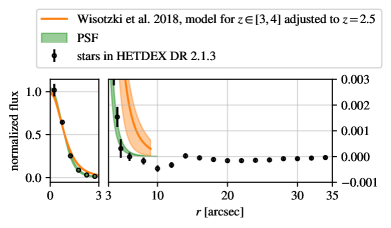
Figure 3: Normalized median radial profile of 3795 stars in our observations (black points) compared to the PSF model (green). The model is a Moffat function with $\beta=3$ and $1.2^{\prime\prime}\leq\mathrm{FWHM}\leq 1.4^{\prime\prime}$. The orange shaded area is the best-fit model from Wisotzki et al. (2018) for halos at $3<z<4$ adjusted to our observation and normalized.The right panel is a continuation of the left panel in radius but covering a smaller range in flux. The radial profile of the stars is negative at $r\gtrsim 5^{\prime\prime}$ because of small errors in the background light correction.

4 Results

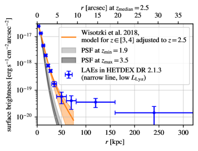
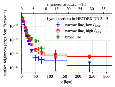
Figure 4: Left: Median surface brightness profile of our LAE sample (blue, $\mathrm{FWHM}_{\mathrm{Ly}\alpha}<1000\,\mathrm{km}\,\mathrm{s}^{-1}$ and $L_{\mathrm{Ly}\alpha}<10^{43}\,\mathrm{erg}\,\mathrm{s}^{-1}$) after subtracting the background surface brightness. The gray shaded area shows the PSF in the observations at the minimum and maximum redshift. The orange profile is the best-fit model in Wisotzki et al. (2018) for LAEs at $3<z<4$, adjusted to our observations and rescaled to match the flux of our galaxies in the core. Our measured radial profile agrees well with this model within $80\,\mathrm{kpc}$, but is flatter at larger radii. Right: Comparison of the median surface brightness profile of the LAE sample (blue) to those with broad lines (green diamonds) and narrow lines and high luminosities (red squares). The background surface brightness values of each sample have been subtracted.

The left panel of Figure 4 displays the median surface brightness profile around our set of LAEs (blue, NLLL sample). The PSF in our observations is shown as a comparison. This median surface brightness profile is clearly more extended than the profile of a point source and shows significant emission of $(3.6\pm 1.3)\times 10^{-20}\,\mathrm{erg}\,\mathrm{s}^{-1}\,\mathrm{cm}^{-2}\,\mathrm{arcsec}^{-2}$ out to $160\,\mathrm{kpc}$. The median profile of continuum emission at longer wavelengths than is consistent with the PSF, but it has insufficient S/N for a meaningful comparison.

The right panel of Figure 4 shows the comparison of the median radial profiles of the three samples: the LAE/NLLL sample (blue), the NLHL sample (red) and the BL sample (green). The narrow-line samples have similar shapes, while the BL sample is flatter at intermediate radii ($25\,\mathrm{kpc}\leq r\leq 60\,\mathrm{kpc}$). Both the NLHL and the BL samples have a higher overall surface brightness than the LAE/NLLL sample, suggesting that the effect of potential AGN contamination in the LAE sample is a higher overall surface brightness and possibly a flattening of the radial profile at intermediate radii. For example, the stacked surface brightness profile of 15 quasars at $z\sim 2$ obtained from narrow-band images yields $(5.5\pm 3.1)\times 10^{-20}$ erg s^-1 cm^-2 arcsec^-2 in a large radial bin of $50<r<500$ kpc (Arrigoni Battaia et al., 2016). While the statistical significance is low, this level of surface brightness is consistent with that of our NLHL sample.

The left panel of Figure 4 compares the profile to the best-fit model for the stack of LAEs at $3<z<4$ reported in Wisotzki et al. (2018). This model consists of a point-like profile proportional to the PSF plus a halo profile following a Sérsic function. The point-like contribution has a total flux $F_{\mathrm{ps}}=\left(232\pm 50\right)\times 10^{-20}\,\mathrm{erg}\,\mathrm{s}^{-1}\,\mathrm{cm}^{-2}$ and $\mathrm{FWHM}=0.703^{\prime\prime}$ for the MUSE instrument. The Sérsic function has the total flux $F_{\mathrm{h}}=\left(1488\pm 83\right)\times 10^{-20}\,\mathrm{erg}\,\mathrm{s}^{-1}\,\mathrm{cm}^{-2}$, effective radius $r_{\mathrm{eff,h}}=0.86^{\prime\prime}\pm 0.11^{\prime\prime}$, and Sérsic index $n_{\mathrm{h}}=2.8\pm 1.1$.

Before we compare this model with our data, we have to account for several differences between the two data sets. First, our LAE sample is located at lower redshifts ($1.9<z<3.5$) and it is on average much brighter (by a factor of $10$ in luminosity) in than the LAE sample of Wisotzki et al. (2018). Second, VIRUS has a larger PSF and larger fiber diameter than MUSE. To account for the redshift difference we translate the angular separation at $z_{\mathrm{mid}}^{\mathrm{MUSE}}=3.5$ to physical distances and back to the corresponding angular separation at our median redshift $z_{\mathrm{median}}=2.5$ ($10\%$ change in scale). We then convolve the model profile with the median PSF of our observations, i.e., a Moffat function with $\beta=3$ and $\mathrm{FWHM}=1.3^{\prime\prime}$. Since the fibers on VIRUS are larger, we also convolve the model profile with the fiber face (a tophat with radius $0.75^{\prime\prime}$). As our sample of galaxies is brighter, we multiply the model profile by $10.3$ such that the flux in the core ($r\leq 2^{\prime\prime}$) of our measured radial profile and the model match.

The adjusted model agrees qualitatively well with our measured radial profile at $r<80\,\mathrm{kpc}$ despite the differences in redshift and luminosities of the LAE samples. At larger radii, our radial profile becomes flatter than the model. However, the measured radial profile from Wisotzki et al. (2018) is also above the fitted profile by $2\,\sigma$ at $60\,\mathrm{kpc}$, which is consistent with a flatter outer radial profile.

There are three possible reasons for the discrepancy at larger radii. First, an unknown systematic error in our analysis may artificially flatten the radial profile. Second, the smaller field of view of MUSE may cause them to over-subtract extended emission and thereby miss the flattening. Third, the flattening may depend on the luminosity or redshift of the LAE sample and may be stronger for brighter, probably more massive LAEs at lower redshift. To test the second possible reason, we imitate a background subtraction for each VIRUS IFU, which is slightly smaller than the MUSE field of view. This removes the flattening at $r\geq 50\,\mathrm{kpc}$. To investigate a possible luminosity dependence, future studies can expand this analysis to fainter LAEs in HETDEX data. The redshift dependence can be tested by expanding the LAE sample and splitting it into redshift bins.

5 Discussion

5.1 Impact of the Background Subtraction

The main goal of this paper is to measure the shape of the emission around LAEs, which requires the removal of background emission. We subtract background emission in three steps: the sky subtraction (Section 2.1), the continuum subtraction (Section 2.3), and the subtraction of the remaining background surface brightness (Section 3.3). The sky subtraction removes the (biweight) average flux within $18^{\prime}$, which covers $8-9\,\mathrm{Mpc}$ in our redshift range, in each $2\,\textup{\AA}$ wavelength bin. The continuum subtraction removes the median flux within $\Delta\lambda=80\,\textup{\AA}$ in the observed frame, which corresponds to a line-of-sight distance of $12-36\,\mathrm{Mpc}$, of each fiber. The background subtraction removes the median surface brightness of random locations within $18^{\prime}$ or $8-9\,\mathrm{Mpc}$ with the same wavelength and integration-window distribution as the LAEs.

It is difficult to disentangle contributions from sky emission residuals, astronomical foreground objects, and the genuine diffuse background to the subtracted background estimates. Due to these background subtraction procedures we may therefore underestimate the surface brightness. The affected scale is $\sim 10\,\mathrm{Mpc}$, which is almost two orders of magnitude larger than our observed range of the profiles. Hence the uncertainty of the background surface brightness should manifest itself as a constant additive term and does not affect the shape of the profiles.

5.2 Comparison with Theoretical Predictions

Figure 5 compares the median radial profile of the NLLL LAE sample with the prediction for halos from the simulation in Byrohl et al. (2021) at $z=3$. The surface brightness of the simulated halos is integrated over $2.2\,\mathrm{Mpc}$-wide slices along the line of sight. This approach is similar to the integration width of our measurement, which has a median (mean) of $2.7\,\mathrm{Mpc}$ ($2.9\,\mathrm{Mpc}$). To adjust the radial profile from the simulation to our observations, we convolve it with the median PSF and VIRUS fiber face. We then subtract the mean surface brightness in the entire simulation volume ($1.9\times 10^{-20}\,\mathrm{erg}\,\mathrm{s}^{-1}\,\mathrm{cm}^{-2}\,\mathrm{arcsec}^{-2}$) from the simulated radial profiles to emulate the background subtraction in our data analysis. Finally, we multiply the profiles by $(1+3)^{4}/(1+2.5)^{4}\approx 1.7$ to account for surface brightness dimming.

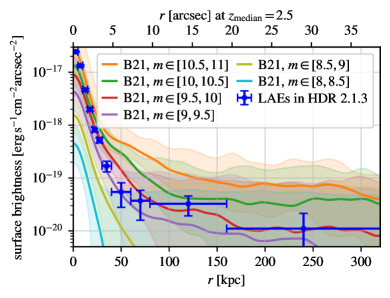
Figure 5: Median surface brightness of the NLLL LAE sample (blue) after subtracting the background, compared to the median simulated surface brightness profiles in Byrohl et al. (2021) in six stellar mass bins ($m=\log_{10}(M_{\star}/M_{\odot})$), adjusted to our observations.

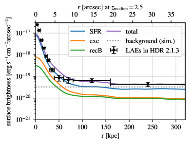
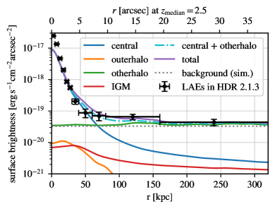
Figure 6: Median surface brightness profile of the NLLL/LAE sample in HETDEX (black) compared to the median surface brightness profiles of simulated galaxies with stellar masses $M_{\star}\in[10^{9.5}M_{\odot},10^{10}M_{\odot}]$ from Byrohl et al. (2021). The dashed gray line indicates the mean surface brightness of the simulation (background (sim.)), which we add to the measured surface brightness profile. Left: Different emission mechanisms of the photons: recombination after photoionization from star formation (SFR, blue), collisional excitation (exc, orange), case-B recombination after including photoionization from an ionizing background (recB, green), and the sum of these (total, purple). SFR dominates the simulated profile at all radii. Right: Different emission origins of the photons: the central galaxy in the target dark matter halo (central, blue), the outer parts of this dark matter halo (outerhalo, orange), another dark matter halo than the target halo (otherhalo, green), IGM (red), and the sum of these (total, purple). The sum of the central and otherhalo contributions (cyan dot-dashed line) reproduces the measured surface brightness profile well except in the core ($r<10\,\mathrm{kpc}$).

This figure displays the median radial profiles of simulated galaxies in six stellar mass ranges between $10^{8}M_{\odot}$ and $10^{11}M_{\odot}$. Our measurements are consistent with the simulated ones; in detail, however, our measured surface brightness profile is steeper than the profiles from the simulation at $r\lesssim 50\,\mathrm{kpc}$.

The Byrohl et al. (2021) simulation finds that most photons illuminating halos originate from star-forming regions within the central galaxy or, at large radii, nearby galaxies, which are scattered in the CGM/IGM. Other emission mechanisms and emission origins contribute less to the total median profile. Figure 6 compares the measured surface brightness profile with the median profiles of individual emission mechanisms and emission origins from simulated galaxies with $M_{\star}\in[10^{9.5}M_{\odot},10^{10}M_{\odot}]$. For an informative comparison, the mean Lya surface brightness from the simulation (“background (sim.)”) is added to the measured profile, as the mean surface brightness for individual simulated components was not available.

The left panel shows different emission mechanisms. SFR dominates the simulated surface brightness profile at all radii.

The right panel presents different emission origins before scattering of the photons. The sum of the central component and the otherhalo component is close to the measured surface brightness profile, suggesting that photons originating from the outer parts of the dark matter halo and IGM play only a minor role in forming the total profile.

While the level of agreement is impressive, there are small discrepancies. One reason is linked to modeling limitations in the hydrodynamic simulations and their radiative transfer treatment: the lack of coupled ionizing radiation from star-forming regions, the lack of dust modeling, and uncertainty in the intrinsic luminosities within galaxies.

The radiation escaping from the ISM is largely determined by the complex radiative transfer in the ISM’s multiphase state that remains unresolved in the simulation. Along with large uncertainties on the intrinsic luminosity of stellar populations and potential emission from obscured AGN, large uncertainties for the luminosity escaping the ISM exist. The assumed linear scaling between star-formation rate and ISM-escaping luminosity in Byrohl et al. (2021) may not accurately reflect reality. The observations reveal substantial scatter in the scaling relation (Santos et al., 2020; Runnholm et al., 2020). The selection of the galaxies in the observation is also different than in the simulation. We may therefore not reflect a potential bias for the observational sample regarding their star-formation and dust content. Finally, while the simulation uses the mean to convert two-dimensional images to radial profiles, we use the median.

In addition to the comparison to hydrodynamical simulations, we also consider an analytically motivated approach by Kakiichi & Dijkstra (2018), who predict a radial profile following a power law $\propto r^{-2.4}$ for $r\in[20,1000]\,\mathrm{kpc}$. In this approach, only scatterings of photons from the central galaxy in the CGM are considered. We compare this prediction with our measurement by fitting a similar model to our stack. The model consists of a point-like component given by a $\delta$ function times a constant $a$, plus a power-law halo, which we terminate at $r_{0}=1^{\prime\prime}$ ($\approx 8\,\mathrm{kpc}$) to avoid divergence at smaller radii. The profile is therefore given by

$$f(r,\phi)=a\times\delta(r)+b\times\begin{cases}1&\text{if }r<1^{\prime\prime}\\ \left(\frac{r}{{}^{\prime\prime}}\right)^{-2.4}&\text{if }r\geq 1^{\prime\prime}.\end{cases}$$ (1)

We convolve the profile at the median redshift ($z_{\mathrm{median}}=2.5$) with the PSF and VIRUS fiber face and fit to the data by varying the constants $a$ and $b$.

Figure 7 shows the result. The power-law fit agrees well with the data out to $r=80\,\mathrm{kpc}$. At larger radii, it underestimates the surface brightness. Since the model only considers scattering of photons originating from the central galaxy, the flattening of the profile at large radii ($r\gtrsim 100\,\mathrm{kpc}$) may be caused by photons that originate from other dark matter halos, as predicted by Byrohl et al. (2021). The outer surface brightness profile is also consistent with the results of Mas-Ribas & Dijkstra (2016) using the CGM model of Dijkstra & Kramer (2012), further suggesting that the clustering of ionizing sources around the LAEs is an important factor.

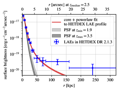
Figure 7: Median surface brightness of the NLLL LAE sample (blue) after subtracting the background. The gray shaded area represents the PSF in the observations at the minimum and maximum redshift. The red line is the least-squares fit of a “core plus power-law” profile motivated by Kakiichi & Dijkstra (2018). The red shaded area shows the 1-$\sigma$ uncertainty of the least-squares fit.

Another reason for the flattening of the profile may be fluorescence from the ultraviolet background. The values predicted by Cantalupo et al. (2005) and Gallego et al. (2018, 2021) are on the order of $10^{-20}\,\mathrm{erg}\,\mathrm{s}^{-1}\,\mathrm{cm}^{-2}\,\mathrm{arcsec}^{-2}$ at $z\sim 3$, which is consistent with the simulations of Byrohl et al. (2021) and the outermost points of our observed profile, but insufficient to explain the surface brightness at intermediate radii. Recent observations hint at the detection of the filamentary structure of the cosmic web traced by at a surface brightness $\sim 10^{-20}-10^{-18}\,\mathrm{erg}\,\mathrm{s}^{-1}\,\mathrm{cm}^{-2}\,\mathrm{arcsec}^{-2}$ at $z\sim 3$ in overdense regions (Umehata et al., 2019; Arrigoni Battaia et al., 2019b; Bacon et al., 2021). Because of their rarity and small volume, they may contribute to, but are unlikely to dominate the median-stacked profile on large scales. Future multi-dimensional analysis similar to Leclercq et al. (2020) can give additional insights on the nature of the extended emission and its link to the Lyman-$\alpha$-emitting cosmic web.

Finally, satellite galaxies or galaxies within the integration window of the line along the line of sight may contribute to the extended emission (Mas-Ribas et al., 2017).

6 Summary

We presented the median radial surface brightness profile of 968 LAEs at $1.9<z<3.5$ that were carefully selected from the DR 2.1.3 of the HETDEX survey. The presence of halos is detected at $(3.6\pm 1.3)\times 10^{-20}\,\mathrm{erg}\,\mathrm{s}^{-1}\,\mathrm{cm}^{-2}\,\mathrm{arcsec}^{-2}$ out to $160\,\mathrm{kpc}$. The potential residual AGN contamination in the LAE sample may increase the overall amplitude of the median radial profile and may flatten the profile in the intermediate radii.

We compared the radial profile with the rescaled model of Wisotzki et al. (2018) for the median radial profile of fainter LAEs at $3<z<4$, which we adjusted to the VIRUS observations. This adjusted model agrees well with our radial profile at $r\lesssim 80\,\mathrm{kpc}$. At larger radii, our measured profile is flatter.

We also compared the radial profile with the median radial surface brightness profiles of galaxies with stellar masses of $10^{8}-10^{11}M_{\odot}$ at $z=3$, taken from the radiative transfer simulation of Byrohl et al. (2021). The simulation results agree well with our measurement at most radii, except at $r<10\,\mathrm{kpc}$ and $30\,\mathrm{kpc}<r<60\,\mathrm{kpc}$. The comparison suggests that our surface brightness profile at $r\lesssim 100$ kpc is dominated by photons emitted in star-forming regions in the central galaxy and, at $r\gtrsim 100\,\mathrm{kpc}$, by photons from galaxies in other dark matter halos. A similar conclusion was reached in Kikuchihara et al. (2021).

Finally, we compared the radial profile with the prediction of Kakiichi & Dijkstra (2018) that the halo is proportional to $r^{-2.4}$ for $r>20\,\mathrm{kpc}$. This power-law profile fits the measured radial profile well at $r\leq 80\,\mathrm{kpc}$. At larger radii our measured profile is flatter. Since Kakiichi & Dijkstra (2018) only considered scattered photons from the central galaxy, this result further suggests that the flattening is due to photons originating from other dark matter halos.

The radiative transfer simulation of Byrohl et al. (2021) predicts that the median profiles of LAEs have similar shapes across redshifts, stellar masses, and luminosities. The similarity of the shapes of our median radial profile and that in Wisotzki et al. (2018), which are at larger redshifts and fainter than our sample, suggests that median profiles at small radii indeed have similar shapes between redshifts $2<z<4$ and across a factor of $10$ in luminosity.

In conclusion, this measurement of faint surface brightness to $>100$ kpc from LAEs shows the high scientific potential of HETDEX observations. The methods to quantify systematic uncertainties developed in this paper will be valuable for intensity mapping (Kovetz et al., 2017; Croft et al., 2018; Kakuma et al., 2021; Kikuchihara et al., 2021) with HETDEX, which will improve constraints on cosmological parameters.

References

- Arrigoni Battaia et al. (2016) Arrigoni Battaia, F., Hennawi, J. F., Cantalupo, S., & Prochaska, J. X. 2016, ApJ, 829, 3, doi: 10.3847/0004-637X/829/1/3
- Arrigoni Battaia et al. (2019a) Arrigoni Battaia, F., Hennawi, J. F., Prochaska, J. X., et al. 2019a, MNRAS, 482, 3162, doi: 10.1093/mnras/sty2827
- Arrigoni Battaia et al. (2019b) Arrigoni Battaia, F., Obreja, A., Prochaska, J. X., et al. 2019b, A&A, 631, A18, doi: 10.1051/0004-6361/201936211
- Astropy Collaboration et al. (2013) Astropy Collaboration, Robitaille, T. P., Tollerud, E. J., et al. 2013, A&A, 558, A33, doi: 10.1051/0004-6361/201322068
- Astropy Collaboration et al. (2018) Astropy Collaboration, Price-Whelan, A. M., Sipőcz, B. M., et al. 2018, AJ, 156, 123, doi: 10.3847/1538-3881/aabc4f
- Bacon et al. (2010) Bacon, R., Accardo, M., Adjali, L., et al. 2010, in Astronomical Telescopes and Instrumentation, ed. I. S. McLean, S. K. Ramsay, & H. Takami (SPIE), 773508–773508–9
- Bacon et al. (2021) Bacon, R., Mary, D., Garel, T., et al. 2021, A&A, 647, A107, doi: 10.1051/0004-6361/202039887
- Beers et al. (1990) Beers, T. C., Flynn, K., & Gebhardt, K. 1990, AJ, 100, 32, doi: 10.1086/115487
- Bond et al. (2010) Bond, N. A., Feldmeier, J. J., Matković, A., et al. 2010, ApJ, 716, L200, doi: 10.1088/2041-8205/716/2/L200
- Borisova et al. (2016) Borisova, E., Cantalupo, S., Lilly, S. J., et al. 2016, ApJ, 831, 39, doi: 10.3847/0004-637X/831/1/39
- Byrohl et al. (2021) Byrohl, C., Nelson, D., Behrens, C., et al. 2021, MNRAS, 506, 5129, doi: 10.1093/mnras/stab1958
- Cai et al. (2017) Cai, Z., Fan, X., Yang, Y., et al. 2017, ApJ, 837, 71, doi: 10.3847/1538-4357/aa5d14
- Cai et al. (2018) Cai, Z., Hamden, E., Matuszewski, M., et al. 2018, ApJ, 861, L3, doi: 10.3847/2041-8213/aacce6
- Cai et al. (2019) Cai, Z., Cantalupo, S., Prochaska, J. X., et al. 2019, ApJS, 245, 23, doi: 10.3847/1538-4365/ab4796
- Camps et al. (2021) Camps, P., Behrens, C., Baes, M., Kapoor, A. U., & Grand, R. 2021, ApJ, 916, 39, doi: 10.3847/1538-4357/ac06cb
- Cantalupo et al. (2014) Cantalupo, S., Arrigoni-Battaia, F., Prochaska, J. X., Hennawi, J. F., & Madau, P. 2014, Nature, 506, 63, doi: 10.1038/nature12898
- Cantalupo et al. (2005) Cantalupo, S., Porciani, C., Lilly, S. J., & Miniati, F. 2005, ApJ, 628, 61, doi: 10.1086/430758
- Christensen et al. (2006) Christensen, L., Jahnke, K., Wisotzki, L., & Sánchez, S. F. 2006, A&A, 459, 717, doi: 10.1051/0004-6361:20065318
- Ciardullo et al. (2013) Ciardullo, R., Gronwall, C., Adams, J. J., et al. 2013, ApJ, 769, 83, doi: 10.1088/0004-637X/769/1/83
- Claeyssens et al. (2019) Claeyssens, A., Richard, J., Blaizot, J., et al. 2019, MNRAS, 489, 5022, doi: 10.1093/mnras/stz2492
- Claeyssens et al. (2022) —. 2022, arXiv e-prints, arXiv:2201.04674. https://arxiv.org/abs/2201.04674
- Croft et al. (2018) Croft, R. A. C., Miralda-Escudé, J., Zheng, Z., Blomqvist, M., & Pieri, M. 2018, MNRAS, 481, 1320, doi: 10.1093/mnras/sty2302
- Croft et al. (2016) Croft, R. A. C., Miralda-Escudé, J., Zheng, Z., et al. 2016, MNRAS, 457, 3541, doi: 10.1093/mnras/stw204
- Dijkstra (2019) Dijkstra, M. 2019, Saas-Fee Advanced Course, 46, 1, doi: 10.1007/978-3-662-59623-4_1
- Dijkstra & Kramer (2012) Dijkstra, M., & Kramer, R. 2012, MNRAS, 424, 1672, doi: 10.1111/j.1365-2966.2012.21131.x
- Erb et al. (2018) Erb, D. K., Steidel, C. C., & Chen, Y. 2018, ApJ, 862, L10, doi: 10.3847/2041-8213/aacff6
- Fardal et al. (2001) Fardal, M. A., Katz, N., Gardner, J. P., et al. 2001, ApJ, 562, 605, doi: 10.1086/323519
- Farina et al. (2019) Farina, E. P., Arrigoni-Battaia, F., Costa, T., et al. 2019, ApJ, 887, 196, doi: 10.3847/1538-4357/ab5847
- Farrow et al. (2021) Farrow, D. J., Sánchez, A. G., Ciardullo, R., et al. 2021, MNRAS, 507, 3187, doi: 10.1093/mnras/stab1986
- Faucher-Giguère et al. (2010) Faucher-Giguère, C.-A., Kereš, D., Dijkstra, M., Hernquist, L., & Zaldarriaga, M. 2010, ApJ, 725, 633, doi: 10.1088/0004-637X/725/1/633
- Feldmeier et al. (2013) Feldmeier, J. J., Hagen, A., Ciardullo, R., et al. 2013, ApJ, 776, 75, doi: 10.1088/0004-637X/776/2/75
- Feltre et al. (2020) Feltre, A., Maseda, M. V., Bacon, R., et al. 2020, A&A, 641, A118, doi: 10.1051/0004-6361/202038133
- Fossati et al. (2021) Fossati, M., Fumagalli, M., Lofthouse, E. K., et al. 2021, MNRAS, 503, 3044, doi: 10.1093/mnras/stab660
- Gaia Collaboration et al. (2016) Gaia Collaboration, Brown, A. G. A., Vallenari, A., et al. 2016, A&A, 595, A2, doi: 10.1051/0004-6361/201629512
- Gallego et al. (2018) Gallego, S. G., Cantalupo, S., Lilly, S., et al. 2018, MNRAS, 475, 3854, doi: 10.1093/mnras/sty037
- Gallego et al. (2021) Gallego, S. G., Cantalupo, S., Sarpas, S., et al. 2021, MNRAS, 504, 16, doi: 10.1093/mnras/stab796
- Gebhardt et al. (2021) Gebhardt, K., Mentuch Cooper, E., Ciardullo, R., et al. 2021, arXiv e-prints, arXiv:2110.04298. https://arxiv.org/abs/2110.04298
- Goto et al. (2009) Goto, T., Utsumi, Y., Furusawa, H., Miyazaki, S., & Komiyama, Y. 2009, MNRAS, 400, 843, doi: 10.1111/j.1365-2966.2009.15486.x
- Gould & Weinberg (1996) Gould, A., & Weinberg, D. H. 1996, ApJ, 468, 462, doi: 10.1086/177707
- Gronke & Bird (2017) Gronke, M., & Bird, S. 2017, ApJ, 835, 207, doi: 10.3847/1538-4357/835/2/207
- Haiman et al. (2000) Haiman, Z., Spaans, M., & Quataert, E. 2000, ApJ, 537, L5, doi: 10.1086/312754
- Harris et al. (2020) Harris, C. R., Millman, K. J., van der Walt, S. J., et al. 2020, Nature, 585, 357, doi: 10.1038/s41586-020-2649-2
- Hayashino et al. (2004) Hayashino, T., Matsuda, Y., Tamura, H., et al. 2004, AJ, 128, 2073, doi: 10.1086/424935
- Hayes et al. (2005) Hayes, M., Östlin, G., Mas-Hesse, J. M., et al. 2005, A&A, 438, 71, doi: 10.1051/0004-6361:20052702
- Hayes et al. (2013) Hayes, M., Östlin, G., Schaerer, D., et al. 2013, ApJ, 765, L27, doi: 10.1088/2041-8205/765/2/L27
- Hayes et al. (2014) Hayes, M., Östlin, G., Duval, F., et al. 2014, ApJ, 782, 6, doi: 10.1088/0004-637X/782/1/6
- Hennawi et al. (2015) Hennawi, J. F., Prochaska, J. X., Cantalupo, S., & Arrigoni-Battaia, F. 2015, Science, 348, 779, doi: 10.1126/science.aaa5397
- Hill et al. (2008) Hill, G. J., Gebhardt, K., Komatsu, E., et al. 2008, Astronomical Society of the Pacific Conference Series, Vol. 399, The Hobby-Eberly Telescope Dark Energy Experiment (HETDEX): Description and Early Pilot Survey Results, ed. T. Kodama, T. Yamada, & K. Aoki, 115
- Hill et al. (2021) Hill, G. J., Lee, H., MacQueen, P. J., et al. 2021, arXiv e-prints, arXiv:2110.03843. https://arxiv.org/abs/2110.03843
- Huang et al. (2021) Huang, Y., Lee, K.-S., Shi, K., et al. 2021, ApJ, 921, 4, doi: 10.3847/1538-4357/ac1acc
- Hunter (2007) Hunter, J. D. 2007, Computing in Science & Engineering, 9, 90, doi: 10.1109/MCSE.2007.55
- Jiang et al. (2013) Jiang, L., Egami, E., Fan, X., et al. 2013, ApJ, 773, 153, doi: 10.1088/0004-637X/773/2/153
- Kakiichi & Dijkstra (2018) Kakiichi, K., & Dijkstra, M. 2018, MNRAS, 480, 5140, doi: 10.1093/mnras/sty2214
- Kakuma et al. (2021) Kakuma, R., Ouchi, M., Harikane, Y., et al. 2021, ApJ, 916, 22, doi: 10.3847/1538-4357/ac0725
- Kikuchihara et al. (2021) Kikuchihara, S., Harikane, Y., Ouchi, M., et al. 2021, arXiv e-prints, arXiv:2108.09288. https://arxiv.org/abs/2108.09288
- Kikuta et al. (2019) Kikuta, S., Matsuda, Y., Cen, R., et al. 2019, PASJ, 71, L2, doi: 10.1093/pasj/psz055
- Kimock et al. (2021) Kimock, B., Narayanan, D., Smith, A., et al. 2021, ApJ, 909, 119, doi: 10.3847/1538-4357/abbe89
- Kollmeier et al. (2010) Kollmeier, J. A., Zheng, Z., Davé, R., et al. 2010, ApJ, 708, 1048, doi: 10.1088/0004-637X/708/2/1048
- Kovetz et al. (2017) Kovetz, E. D., Viero, M. P., Lidz, A., et al. 2017, arXiv e-prints, arXiv:1709.09066. https://arxiv.org/abs/1709.09066
- Kusakabe et al. (2022) Kusakabe, H., Verhamme, A., Blaizot, J., et al. 2022, arXiv e-prints, arXiv:2201.07257. https://arxiv.org/abs/2201.07257
- Lake et al. (2015) Lake, E., Zheng, Z., Cen, R., et al. 2015, ApJ, 806, 46, doi: 10.1088/0004-637X/806/1/46
- Leclercq et al. (2017) Leclercq, F., Bacon, R., Wisotzki, L., et al. 2017, A&A, 608, A8, doi: 10.1051/0004-6361/201731480
- Leclercq et al. (2020) Leclercq, F., Bacon, R., Verhamme, A., et al. 2020, A&A, 635, A82, doi: 10.1051/0004-6361/201937339
- Leung et al. (2017) Leung, A. S., Acquaviva, V., Gawiser, E., et al. 2017, ApJ, 843, 130, doi: 10.3847/1538-4357/aa71af
- Martin et al. (2014a) Martin, D. C., Chang, D., Matuszewski, M., et al. 2014a, ApJ, 786, 106, doi: 10.1088/0004-637X/786/2/106
- Martin et al. (2014b) —. 2014b, ApJ, 786, 107, doi: 10.1088/0004-637X/786/2/107
- Mas-Ribas & Dijkstra (2016) Mas-Ribas, L., & Dijkstra, M. 2016, ApJ, 822, 84, doi: 10.3847/0004-637X/822/2/84
- Mas-Ribas et al. (2017) Mas-Ribas, L., Dijkstra, M., Hennawi, J. F., et al. 2017, ApJ, 841, 19, doi: 10.3847/1538-4357/aa704e
- Matsuda et al. (2004) Matsuda, Y., Yamada, T., Hayashino, T., et al. 2004, AJ, 128, 569, doi: 10.1086/422020
- Matsuda et al. (2011) —. 2011, MNRAS, 410, L13, doi: 10.1111/j.1745-3933.2010.00969.x
- Matsuda et al. (2012) —. 2012, MNRAS, 425, 878, doi: 10.1111/j.1365-2966.2012.21143.x
- McCarthy et al. (1987) McCarthy, P. J., Spinrad, H., Djorgovski, S., et al. 1987, ApJ, 319, L39, doi: 10.1086/184951
- Mitchell et al. (2021) Mitchell, P. D., Blaizot, J., Cadiou, C., et al. 2021, MNRAS, 501, 5757, doi: 10.1093/mnras/stab035
- Møller & Warren (1998) Møller, P., & Warren, S. J. 1998, MNRAS, 299, 661, doi: 10.1046/j.1365-8711.1998.01749.x
- Momose et al. (2014) Momose, R., Ouchi, M., Nakajima, K., et al. 2014, MNRAS, 442, 110, doi: 10.1093/mnras/stu825
- Momose et al. (2016) —. 2016, MNRAS, 457, 2318, doi: 10.1093/mnras/stw021
- Nakajima et al. (2018) Nakajima, K., Schaerer, D., Le Fèvre, O., et al. 2018, A&A, 612, A94, doi: 10.1051/0004-6361/201731935
- Nelson et al. (2020) Nelson, D., Sharma, P., Pillepich, A., et al. 2020, MNRAS, 498, 2391, doi: 10.1093/mnras/staa2419
- Östlin et al. (2009) Östlin, G., Hayes, M., Kunth, D., et al. 2009, AJ, 138, 923, doi: 10.1088/0004-6256/138/3/923
- O’Sullivan et al. (2020) O’Sullivan, D. B., Martin, C., Matuszewski, M., et al. 2020, ApJ, 894, 3, doi: 10.3847/1538-4357/ab838c
- Ouchi et al. (2009) Ouchi, M., Ono, Y., Egami, E., et al. 2009, ApJ, 696, 1164, doi: 10.1088/0004-637X/696/2/1164
- Overzier et al. (2001) Overzier, R. A., Röttgering, H. J. A., Kurk, J. D., & De Breuck, C. 2001, A&A, 367, L5, doi: 10.1051/0004-6361:20010041
- Patrício et al. (2016) Patrício, V., Richard, J., Verhamme, A., et al. 2016, MNRAS, 456, 4191, doi: 10.1093/mnras/stv2859
- Planck Collaboration et al. (2020) Planck Collaboration, Aghanim, N., Akrami, Y., et al. 2020, A&A, 641, A6, doi: 10.1051/0004-6361/201833910
- Ramsey et al. (1994) Ramsey, L. W., Sebring, T. A., & Sneden, C. A. 1994, Society of Photo-Optical Instrumentation Engineers (SPIE) Conference Series, Vol. 2199, Spectroscopic survey telescope project, ed. L. M. Stepp, 31–40, doi: 10.1117/12.176221
- Rasekh et al. (2021) Rasekh, A., Melinder, J., Östlin, G., et al. 2021, arXiv e-prints, arXiv:2110.01626. https://arxiv.org/abs/2110.01626
- Rauch et al. (2008) Rauch, M., Haehnelt, M., Bunker, A., et al. 2008, ApJ, 681, 856, doi: 10.1086/525846
- Reuland et al. (2003) Reuland, M., van Breugel, W., Röttgering, H., et al. 2003, ApJ, 592, 755, doi: 10.1086/375619
- Runnholm et al. (2020) Runnholm, A., Hayes, M., Melinder, J., et al. 2020, ApJ, 892, 48, doi: 10.3847/1538-4357/ab7a91
- Santos et al. (2020) Santos, S., Sobral, D., Matthee, J., et al. 2020, MNRAS, 493, 141, doi: 10.1093/mnras/staa093
- Shibuya et al. (2018) Shibuya, T., Ouchi, M., Konno, A., et al. 2018, PASJ, 70, S14, doi: 10.1093/pasj/psx122
- Smit et al. (2017) Smit, R., Swinbank, A. M., Massey, R., et al. 2017, MNRAS, 467, 3306, doi: 10.1093/mnras/stx245
- Smith & Jarvis (2007) Smith, D. J. B., & Jarvis, M. J. 2007, MNRAS, 378, L49, doi: 10.1111/j.1745-3933.2007.00318.x
- Smith et al. (2008) Smith, D. J. B., Jarvis, M. J., Lacy, M., & Martínez-Sansigre, A. 2008, MNRAS, 389, 799, doi: 10.1111/j.1365-2966.2008.13580.x
- Smith et al. (2009) Smith, D. J. B., Jarvis, M. J., Simpson, C., & Martínez-Sansigre, A. 2009, MNRAS, 393, 309, doi: 10.1111/j.1365-2966.2008.14232.x
- Spinoso et al. (2020) Spinoso, D., Orsi, A., López-Sanjuan, C., et al. 2020, A&A, 643, A149, doi: 10.1051/0004-6361/202038756
- Steidel et al. (2000) Steidel, C. C., Adelberger, K. L., Shapley, A. E., et al. 2000, ApJ, 532, 170, doi: 10.1086/308568
- Steidel et al. (2011) Steidel, C. C., Bogosavljević, M., Shapley, A. E., et al. 2011, ApJ, 736, 160, doi: 10.1088/0004-637X/736/2/160
- Swinbank et al. (2007) Swinbank, A. M., Bower, R. G., Smith, G. P., et al. 2007, MNRAS, 376, 479, doi: 10.1111/j.1365-2966.2007.11454.x
- Umehata et al. (2019) Umehata, H., Fumagalli, M., Smail, I., et al. 2019, Science, 366, 97, doi: 10.1126/science.aaw5949
- van de Voort et al. (2019) van de Voort, F., Springel, V., Mandelker, N., van den Bosch, F. C., & Pakmor, R. 2019, MNRAS, 482, L85, doi: 10.1093/mnrasl/sly190
- van Ojik et al. (1997) van Ojik, R., Roettgering, H. J. A., Miley, G. K., & Hunstead, R. W. 1997, A&A, 317, 358. https://arxiv.org/abs/astro-ph/9608092
- Virtanen et al. (2020) Virtanen, P., Gommers, R., Oliphant, T. E., et al. 2020, Nature Methods, 17, 261, doi: 10.1038/s41592-019-0686-2
- Weidinger et al. (2004) Weidinger, M., Møller, P., & Fynbo, J. P. U. 2004, Nature, 430, 999, doi: 10.1038/nature02793
- Weidinger et al. (2005) Weidinger, M., Møller, P., Fynbo, J. P. U., & Thomsen, B. 2005, A&A, 436, 825, doi: 10.1051/0004-6361:20042304
- Wisotzki et al. (2016) Wisotzki, L., Bacon, R., Blaizot, J., et al. 2016, A&A, 587, A98, doi: 10.1051/0004-6361/201527384
- Wisotzki et al. (2018) Wisotzki, L., Bacon, R., Brinchmann, J., et al. 2018, Nature, 562, 229, doi: 10.1038/s41586-018-0564-6
- Wu et al. (2020) Wu, J., Jiang, L., & Ning, Y. 2020, ApJ, 891, 105, doi: 10.3847/1538-4357/ab7333
- Xue et al. (2017) Xue, R., Lee, K.-S., Dey, A., et al. 2017, ApJ, 837, 172, doi: 10.3847/1538-4357/837/2/172
- Yang et al. (2010) Yang, Y., Zabludoff, A., Eisenstein, D., & Davé, R. 2010, ApJ, 719, 1654, doi: 10.1088/0004-637X/719/2/1654
- Zhang et al. (2020) Zhang, H., Ouchi, M., Itoh, R., et al. 2020, ApJ, 891, 177, doi: 10.3847/1538-4357/ab7917
- Zhang et al. (2021) Zhang, Y., Ouchi, M., Gebhardt, K., et al. 2021, arXiv e-prints, arXiv:2105.11497. https://arxiv.org/abs/2105.11497
- Zheng et al. (2011) Zheng, Z., Cen, R., Weinberg, D., Trac, H., & Miralda-Escudé, J. 2011, ApJ, 739, 62, doi: 10.1088/0004-637X/739/2/62