Decay of multiple dark matter particles to dark radiation in different epochs does not alleviate the Hubble tension

Abstract

Decaying cold dark matter (CDM) has been considered as a mechanism to tackle the tensions in the Hubble expansion rate and the clustering of matter. However, polarization measurements of the cosmic microwave background (CMB) severely constrain the fraction of dark matter decaying before recombination, and lensing of the CMB anisotropies by large-scale structure set strong constraints on dark matter decaying after recombination. Together, these constraints make an explanation of the Hubble tension in terms of decaying dark matter unlikely. In response to this situation, we investigate whether a dark matter ensemble with CDM particles decaying into free streaming dark radiation in different epochs can alleviate the problem. We find that it does not.

I Introduction

Shortly after high-resolution experiments heralded the field of precision cosmology, low- and high-redshift observations gave rise to a tension in the measurement of the present-day expansion rate of the Universe ($H_{0}$) and the clustering of matter ($S_{8}$). Assuming the standard $\Lambda$ cold dark matter (CDM) cosmological model, the Planck Collaboration examined anisotropies in the cosmic microwave background (CMB) temperature and polarization fields to infer that the Universe is expanding $67.27\pm 0.60$ kilometers per second faster every megaparsec Planck:2018vyg , whereas the most influential measurements of the late Universe by the SH0ES experiment, peg the Hubble constant at $73.2\pm 1.3~{}{\rm km/s/Mpc}$ Riess:2020fzl . For a recent compilation of other late Universe $H_{0}$ measurements, see e.g. DiValentino:2020zio . When the late Universe measurements are averaged in different combinations, the $H_{0}$ values disagree between $4.4\sigma$ and $6.3\sigma$ with the one reported by the Planck Collaboration Verde:2019ivm . The statistical significance of the mismatch between the high $S_{8}$ value estimated by the Planck Collaboration assuming $\Lambda$CDM and the lower value preferred by cosmic shear measurements is somewhat smaller at $\sim 3\sigma$ DiValentino:2020vvd . It is desirable that the $H_{0}$ and $S_{8}$ tensions be addressed simultaneously, but currently none of the proposed models have done so to a satisfactory degree DiValentino:2021izs ; Schoneberg:2021qvd ; Anchordoqui:2021gji .

In CMB parlance, $\theta_{\rm LS}\equiv r_{\rm LS}/D_{M}(z_{\rm LS})$ is the angular size of the sound horizon at the last scattering (LS) surface, where $r_{\rm LS}$ is the linear size of the sound horizon (i.e., the comoving distance traveled by a sound wave from the beginning of the universe until recombination) and $D_{M}(z_{\rm LS})=\int_{0}^{z_{\rm LS}}dz/H(z)$ is the comoving angular diameter distance from a present day observer to $z_{\rm LS}$, with $H(z)$ the redshift-dependent expansion rate. Since $\theta_{\rm LS}$ can be precisely measured from the locations of the acoustic peaks in the CMB temperature and polarization anisotropy spectra, given $r_{\rm LS}$, an estimate of $H_{0}$ follows from $D_{M}(z_{\rm LS})$.

Several models in which an unstable component of multicomponent CDM decays into dark radiation have been proposed to relax the $H_{0}$ and $S_{8}$ tensions Menestrina:2011mz ; Hooper:2011aj ; Gonzalez-Garcia:2012djt ; Berezhiani:2015yta ; Vattis:2019efj ; Enqvist:2015ara ; Abellan:2020pmw ; Abellan:2021bpx . These models can be classified according to the particle’s decay width $\Gamma$. For models with short-lived particles, viz. $\Gamma\gtrsim 10^{6}~{}{\rm Gyr}^{-1}$, CDM is depleted into dark radiation at redshifts $z>z_{\rm LS}$, thereby increasing the expansion rate while reducing the comoving linear size of the sound horizon Menestrina:2011mz ; Hooper:2011aj ; Gonzalez-Garcia:2012djt . Since the value of $\theta_{\rm LS}$ is a CMB observable that must be kept fixed, a reduction of $r_{\rm LS}$ simultaneously decreases $D_{M}(z_{\rm LS})$ and increases $H_{0}$. For models with long-lived particles, CDM is depleted into radiation at $z<z_{\rm LS}$ and matter-dark energy equality is shifted to earlier times than in $\Lambda$CDM, allowing for an increase in $H_{0}$ at late times Berezhiani:2015yta ; Vattis:2019efj . Furthermore, two-body decays that transfer energy from CDM to dark radiation at redshift $z<z_{\rm LS}$ reduce the matter content in the late universe to accommodate local measurements of $S_{8}$ Enqvist:2015ara ; Abellan:2020pmw ; Abellan:2021bpx . For $\Gamma\gtrsim H_{0}\sim 0.7~{}{\rm Gyr}^{-1}$, most of the unstable dark matter particles have disappeared by $z=3$ (with implications for IceCube observations if sterile neutrinos play the role of dark radiation Anchordoqui:2015lqa ; Anchordoqui:2021dls ), whereas for $\Gamma\lesssim H_{0}$, only a fraction of the unstable dark matter particles have had time to disappear.

A point worth noting is that the most recent CMB data severely constrain the fraction of unstable dark matter in all of these models Chudaykin:2016yfk ; Poulin:2016nat ; Clark:2020miy ; Chudaykin:2017ptd ; Nygaard:2020sow ; Anchordoqui:2020djl . On the one hand, the fraction of short-lived particles is strongly constrained by CMB polarization measurements Nygaard:2020sow ; Anchordoqui:2020djl . On the other hand, the lack of dark matter at low redshifts reduces the CMB lensing power which is at odds with data from Planck Chudaykin:2016yfk ; Poulin:2016nat ; Clark:2020miy . The inclusion of measurements of baryon acoustic oscillations (BAO) yields even tighter constraints on the fraction of long-lived particles Chudaykin:2017ptd ; Nygaard:2020sow . All in all, current bounds on the fraction of decaying particles in the hidden sector make a solution to the $H_{0}$ tension in terms of decaying dark matter unlikely. It remains to be seen, however, whether a combination of these scenarios, with multiple dark matter particles decaying in different epochs, can ameliorate this tension.

Dynamical dark matter (DDM) provides a framework to model the decay of a dark matter ensemble across epochs Dienes:2011ja . In the DDM framework, dark matter stability is replaced by a balancing of lifetimes against cosmological abundances in an ensemble of individual dark matter components with different masses, lifetimes, and abundances. This DDM ensemble collectively describes the observed dark matter abundance. How observations of Type-Ia SNe Scolnic:2017caz can constrain ensembles comprised of a large number of cold particle species that decay primarily into dark radiation was explored in Ref. Desai:2019pvs . In this paper, we investigate whether CDM particles decaying in different epochs can alleviate the $H_{0}$ tension.

II Cosmology of dark matter ensembles

Inferences from astronomical and cosmological observations are made under the assumption that the Universe is homogeneous and isotropic, and consequently its evolution can be characterized by a spatially flat Friedmann-Robertson-Walker line element,

$$ds^{2}=-dt^{2}+a^{2}(t)\ \left(dx^{2}+dy^{2}+dz^{2}\right),$$ (1)

where $(t,x,y,z)$ are comoving coordinates and $a(t)$ is the expansion scale factor of the universe.

The dynamics of the universe is governed by the Friedmann equation for the Hubble parameter $H$,

$$H^{2}(a)=\frac{8\pi G}{3}\sum_{i}\rho_{i}(a)\,,$$ (2)

where $G$ is the gravitational constant and the sum runs over the energy densities $\rho_{i}$ of the various components of the cosmic fluid: dark energy (DE), dark matter (DM), baryons ($b$), photons ($\gamma$), and neutrinos ($\nu$). In terms of the present day value of the critical density $\rho_{\rm crit,0}=3H_{0}^{2}/(8\pi G)$, the Friedmann equation can be recast as

$$H^{2}(a) = H_{0}^{2}\ \Bigg{[}\Omega_{b}\,a^{-3}+\Omega_{\gamma}\,a^{-4}+\frac{\rho_{\nu}(a)}{\rho_{\rm crit,0}}\Omega_{\rm DE}\exp\left(3\;\int_{a}^{1}\frac{1+w}{a^{\prime}}da^{\prime}\right)+\frac{\rho_{\rm DM}(a)}{\rho_{\rm crit,0}}\;\Bigg{]}\;,$$ (3)

where $\Omega_{i}=\rho_{i,0}/\rho_{\rm crit,0}$ denote the present-day density fractions, and the subscript $0$ indicates quantities evaluated today, with $a_{0}=1$. The energy densities of non-relativistic matter and radiation scale as $a^{-3}$ and $a^{-4}$ respectively. The scaling of $\Omega_{\rm DE}$ is usually described by an “equation-of-state” parameter $w\equiv p_{\rm DE}/\rho_{\rm DE}$, the ratio of the spatially-homogeneous dark energy pressure $p_{\rm DE}$ to its energy density $\rho_{\rm DE}$. The observed cosmic acceleration demands $w<-1/3$. Herein we ascribe the DE component to the cosmological constant $\Lambda$, for which $w=-1$, and assume three families of massless (Standard Model) neutrinos. With this in mind, Eq. (3) can be simplified to

$$H^{2}(a)=H_{0}^{2}\Bigg{[}\Omega_{b}\ a^{-3}+(\Omega_{\gamma}+\Omega_{\nu})\,a^{-4}+\Omega_{\Lambda}+\frac{\rho_{\rm DM}(a)}{\rho_{\rm crit,0}}\;\Bigg{]}\;.$$ (4)

We consider a hidden sector with multiple dark matter particles with different lifetimes. The ensemble is made up of $N$ particle species $\chi_{n}$, with total decay widths $\Gamma_{n}\equiv 1/\tau_{n}$, where $n=1,2,\cdots,N$. They decay via $\chi_{n}\to\psi\overline{\psi}$, where $\psi$ is a massless dark sector particle that behaves as dark radiation. The initial abundances $\rho_{n}(a_{\rm prod})$, are regulated by early universe processes and are fixed at $a_{\rm prod}\ll a_{\rm LS}$, with $t_{\rm prod}\ll\tau_{n}$, where $a_{\rm LS}$ is the scale factor at last scattering. For simplicity, we assume that all particles in the ensemble are cold, in the sense that their equation-of-state parameter may be taken to be $w_{n}\approx 0$ for all $t>t_{\rm prod}$.

The evolution of the energy densities $\rho_{n}$ of each particle species and of the massless dark field $\rho_{\psi}$ are driven by the Boltzmann equations,

$$\frac{d\rho_{n}}{dt}+3H\rho_{n}=-\Gamma_{n}\rho_{n}$$ (5)

and

$$\frac{d\rho_{\psi}}{dt}+4H\rho_{\psi}=\sum_{n=1}^{N}\Gamma_{n}\rho_{n}\,,$$ (6)

respectively. In Eqs. (5) and (6) we have omitted the collision terms associated with inverse decay processes of the type $\psi\overline{\psi}\rightarrow\chi_{n}$, because their effect on the $\rho_{n}$ and $\rho_{\psi}$ is negligible. Our goal is to solve these equations to obtain the evolution of the Hubble parameter (Eq. 4), which may then be used to determine the free parameters of the model by imposing the following constraints derived from cosmological observations:

• The baryonic matter and radiation densities ParticleDataGroup:2020ssz ,

  • $\left.\Omega_{b}h_{0}^{2}\right|_{\rm exp}=0.02237(15)$,

  • $\left.\Omega_{\gamma}h_{0}^{2}\right|_{\rm exp}=2.473\times 10^{-5}(T_{\gamma,0}/2.7255\,\mathrm{K})^{4}$, where $T_{\gamma,0}=2.7255(6)\,\mathrm{K}$ is the current temperature of the CMB photons,

  with $H_{0}=100~{}h_{0}~{}{\rm km/s/Mpc}$. A point worth noting is that the baryon density inferred from Planck data is in good agreement with the $\Omega_{b}h_{0}^{2}$ determination from measurements of the primordial deuterium abundance (D/H) in conjunction with big bang nucleosynthesis (BBN) theory Cooke:2016rky ; Mossa:2020gjc . We have verified that variations of $\Omega_{b}h_{0}^{2}$ within observational and modeling uncertainties do not change our results.

• The neutrino number density per flavor $\alpha$ is fixed by the temperature of the CMB photons,

  $$n_{\nu_{\alpha},0}=\frac{3}{11}n_{\gamma,0}=\frac{6\,\zeta(3)}{11\pi^{2}}T^{3}_{\gamma,0}\sim 113~{}{\rm cm^{-3}}\,.$$ (7)

  The energy density depends on the neutrino masses $m_{\nu}$. Under our assumption that $m_{\nu}\ll T_{\nu,0}=(4/11)^{1/3}\,T_{\gamma,0}$,

  $$\rho_{\nu_{\alpha},0}=\frac{7\pi^{2}}{120}\left(\frac{4}{11}\right)^{4/3}\,T^{4}_{\gamma,0}\,.$$ (8)

• The extra relativistic degrees-of-freedom in the early universe is characterized by the number of “equivalent” light neutrino species,

  $$N_{\rm eff}\equiv\frac{\rho_{\rm R}-\rho_{\gamma}}{\rho_{\nu}}\,,$$ (9)

  in units of the density of a single Weyl neutrino $\rho_{\nu}$, where $\rho_{\rm R}$ is the total energy density in relativistic particles and $\rho_{\gamma}$ is the energy density of photons Steigman:1977kc . For three families of massless (Standard Model) neutrinos, $N_{\rm eff}^{\rm SM}=3.046$ Mangano:2005cc . Combining CMB and BAO data with predictions from BBN, the Planck Collaboration reported $N_{\rm eff}=3.04\pm 0.22$ at the 95% CL Planck:2018vyg , which corresponds to $\Delta N_{\rm eff}=N_{\rm eff}-N_{\rm eff}^{\rm SM}<0.214$. In our model, $\rho_{R}=\rho_{\nu}+\rho_{\psi}$, so that

  $$\Delta N_{\rm eff}=\frac{8}{7}\left(\frac{11}{4}\right)^{4/3}\frac{\rho_{\psi}(a_{\rm LS})}{\rho_{\gamma}(a_{\rm LS})}.$$ (10)

  The above $95\%\,\mathrm{CL}$ bound requires our model to satisfy $\rho_{\psi}(a_{\rm LS})\lesssim 0.1\ \rho_{\gamma}(a_{\rm LS})$.

• Setting $\rho_{\rm DM}=\rho_{\psi}+\sum_{n=1}^{N}\rho_{n}$, the evolution of the Hubble parameter must accommodate a diverse set of measurements of $H(z)$ at $z\leq 2.35$, described in more detail in §IV.1. While some of those measurements are independent of any cosmological model, others rely on BAO data, and a prior on the radius of the sound horizon evaluated at the end of the baryon-drag epoch ($r_{d}$) ought to be imposed. This value may be separately obtained from a model dependent analysis of early universe CMB data ($r_{d,e}$), or from model independent parameterizations constrained by low redshift probes ($r_{d,l}$). We employ the measurement for $r_{d,e}$ in model 1 (base $\rm\Lambda CDM$ model with $N_{\rm eff}$) Anchordoqui:2021gji : $r_{d,e}=(148.3\pm 1.9)\,\mathrm{Mpc}$. For the local universe measurement, we use $r_{d,l}=(137\pm 3^{\rm stat}\pm 2^{\rm syst})~{}{\rm Mpc}$ Arendse:2019hev .

III Setting up the system of Boltzmann equations

In order to study the low redshift behavior of the Hubble parameter, we need to solve the system of first order non-linear differential equations formed by the $N+1$ Boltzmann equations for the dark sector, together with the Friedmann equation. Although Eq. (5) can be analytically reduced to $\rho_{n}a^{3}\exp(\Gamma_{n}t)={\rm constant}$, this does not provide an advantage in solving the system, since $t\sim\int da/aH$ and $H$ is a function of $\rho_{n}$ and $\rho_{\psi}$. We therefore proceed to a fully numerical solution of the problem.

We ease this task by defining $\tilde{\rho}_{i}\equiv\rho_{i}/\rho_{{\rm crit},0}$ and $\tilde{\Gamma}_{i}\equiv\Gamma_{i}/({100\,{\rm km/s/Mpc}})$ to render the equations and free parameters dimensionless. Also, we use $u\equiv\ln a$ as an independent variable. This allows to rewrite Eqs. (4), (5) and (6) as

$$\frac{d\tilde{\rho}_{n}}{du}+3\tilde{\rho}_{n}+\frac{\tilde{\Gamma}_{n}\tilde{\rho}_{n}}{\,h(u)}=0\,,$$ (11a)

$$\frac{d\tilde{\rho}_{\psi}}{du}+4\tilde{\rho}_{\psi}-\frac{1}{\,h(u)}\sum_{n=1}^{N}{\tilde{\Gamma}_{n}\tilde{\rho}_{n}}=0\,,$$ (11b)

$$h^{2}(u)=h_{0}^{2}\left(\Omega_{b}\,e^{-3u}+\Omega_{r}\,e^{-4u}+\Omega_{\Lambda}+\tilde{\rho}_{\rm DM}(u)\right)\,.$$ (11c)

The system of equations must be supplemented with $N+1$ initial conditions, i.e., $u_{\rm prod}$. We define $\tilde{\rho}_{1,\rm prod}\equiv\tilde{\rho}_{1}(u_{\rm prod})$, and assume that the production of dark radiation in the very early universe is negligible, so that $\tilde{\rho}_{\psi}(u_{\rm prod})=0$.

It is worth mentioning that Eq. (11c) satisfies $h(0)=h_{0}$ only if $\Omega_{b}+\Omega_{r}+\Omega_{\Lambda}+\Omega_{\rm DM}=1$, where $\Omega_{\rm DM}\equiv\tilde{\rho}_{\rm DM}(0)$. This is not the case for arbitrary initial conditions so this consistency condition must be imposed after solving the system of equations. To do so, we first set $\Omega_{b}\,h_{0}^{2}$ and $\Omega_{r}\,h_{0}^{2}$ to their measured values, fix all model parameters save one, and then vary the remaining parameter until the consistency condition is met. We choose the initial density $\tilde{\rho}_{1,{\rm prod}}$ to be determined by the consistency condition, and is given by the root of the function,

$$\mathcal{G}(\tilde{\rho}_{1,{\rm prod}})\equiv\alpha+h_{0}^{2}\left(\Omega_{\Lambda}+\Omega_{\rm DM}-1\right),$$ (12)

where $\left.\alpha\equiv\Omega_{b}\,h_{0}^{2}+\Omega_{r}\,h_{0}^{2}\right|_{\rm exp}\approx 0.0224$. Note that $\tilde{\rho}_{\rm DM,0}$ is implicitly dependent on $\tilde{\rho}_{1,{\rm prod}}$.

IV Observational datasets and statistical methodology

IV.1 The data

In the following we provide a succinct description of the data we use to constrain the dark matter ensembles.

IV.1.1 Supernovae magnitudes

We use the Pantheon Sample Scolnic:2017caz , consisting of a combination of high quality measurements of supernovae spectrally confirmed to be type Ia, and cross calibrated between different experiments to reduce systematics. Specifically, we use $(z,m_{B})$ data from 1048 supernovae with $z\in[0.01,2.26]$ to constrain the luminosity distance,

$$D_{L}(z)\equiv(1+z)\,c\int_{0}^{z}\frac{dz^{\prime}}{H(z^{\prime})}\,,$$ (13)

which may also be written as

$$d(z)\equiv(1+z)\int_{0}^{z}\frac{dz^{\prime}}{h(z^{\prime})}\,,$$ (14)

and are related by $d(z)=D_{L}(z)100\,\mathrm{km/s/Mpc}/c$. In terms of the distance modulus, $D_{L}=10^{1+(m_{B}-M_{B})/5}\,\mathrm{pc}$, where $m_{B}$ and $M_{B}$ are the apparent and absolute magnitudes of the source. This may be rewritten as $m_{B}=M_{B}+A+5\log d(z)$, with $A=5\log[c/({\mathrm{m\,s^{-1}}})]$.

IV.1.2 Hubble parameter

As a direct measurement of the Hubble parameter at low redshift, we use Observational Hubble Data (OHD) inspired by Table III of Cai:2021weh . The data use the relative ages of nearby (in $z$) galaxies, to obtain an approximation to $dz/dt$, from which the Hubble parameter can be estimated as described in Ref. Jimenez:2001gg . The measurements are solely dependent on models that describe the spectral evolution of stellar populations and, therefore, independent of any cosmological model. The data we use is derived using the model in Bruzual:2003tq , and contains 30 data points from Refs. Jimenez:2003iv ; Simon:2004tf ; Stern:2009ep ; Moresco:2012jh ; Zhang:2012mp ; Moresco:2015cya ; Moresco:2016mzx with $z\in[0.07,1.965]$.

IV.1.3 Large scale structure

We include the large scale structure information in BAO data. Following Cai:2021weh , we use data from the 6dF Galaxy Survey Beutler:2011hx , the Sloan Digital Sky Survey (SDSS) Ross:2014qpa ; BOSS:2016zkm ; Ata:2017dya ; deSainteAgathe:2019voe ; Blomqvist:2019rah ; Bautista:2020ahg ; Gil-Marin:2020bct ; deMattia:2020fkb ; Tamone:2020qrl ; Neveux:2020voa ; Hou:2020rse ; duMasdesBourboux:2020pck , and Dark Energy Survey (DES) DES:2021esc , totaling 35 measurements with $z\in[0.106,2.35]$. The quantities $r_{d}/D_{V}$, $D_{V}/r_{d}$, $D_{A}/r_{d}$, $D_{H}/r_{d}$, $D_{M}/r_{d}$ and $H\,r_{d}$ are directly measured from BAO data. The different distances are related by $D_{H}=c/H$, $D_{M}=D_{L}/(1+z)$, $D_{A}=D_{L}/(1+z)^{2}$, and $D_{V}^{3}=zD_{M}^{2}D_{H}$. These data points must be supplemented by an experimental value for $r_{d}$ which is either the local ($r_{d,l}$) or the early universe ($r_{d,e}$) value, introduced in §II.

IV.1.4 Hubble constant

As a last data point, we include the expansion rate of the local ($z\approx 0$) Universe, $H_{0}=(73.2\pm 1.3)\,\mathrm{km/s/Mpc}$ Riess:2020fzl . This data point is only included in the analysis with the local value $r_{d,l}\approx 137\,\mathrm{Mpc}$.

IV.2 The likelihood

We now introduce the ingredients of our data analysis. Assuming Gaussian errors in the measurements, we write the likelihood of the data given the cosmological model as

$$L=\mathcal{A}\prod_{p=1}^{4}\exp\left(-\frac{\chi_{p}^{2}}{2}\right)\,,$$ (15)

where the partial chi-squared,

$$\chi_{p}^{2}=\sum_{i=1}^{\mathcal{N}_{p}}\left(\frac{y_{p,i}-\mathcal{F}_{p}(z_{p,i})}{\sigma_{p,i}}\right)^{2}\,,$$ (16)

is obtained from the data of the $p^{\rm th}$ combined sample, and $\mathcal{A}$ is a normalization constant which depends on whether the local or the early universe value of $r_{d}$ is used. Specifically, $\log\mathcal{A}_{l}\approx 1208$ and $\log\mathcal{A}_{e}\approx 1212$. These combined samples are obtained from the original data variables (collectively called $x$ below). In the following, $k\equiv 100\,\mathrm{km/s/Mpc}$:

1. $(z,h)$ from OHD and BAO, with $\mathcal{F}_{1}(z)=h(z)$:

   $\quad\quad x\quad\quad$	$\quad\quad y_{1,i}\quad\quad$	$\sigma_{1,i}^{2}$
   $H$	$x_{i}/k$	${\sigma_{x}}_{i}^{2}/k^{2}$
   $H\,r_{d}$	$\frac{x_{i}}{k\,\tilde{r}_{d}}$	$(k\,\tilde{r}_{d})^{-2}\left({\sigma_{x}}_{i}^{2}+\frac{x^{2}}{\tilde{r}_{d}^{2}}\sigma_{\tilde{r}_{d}}^{2}\right)$
   $D_{H}/r_{d}$	$\frac{c}{k\,\tilde{r}_{d}\,x_{i}}$	$\left(\frac{c}{k\,\tilde{r}_{d}\,x_{i}}\right)^{2}\left(\frac{{\sigma_{x}}_{i}^{2}}{x_{i}^{2}}+\frac{\sigma_{\tilde{r}_{d}}^{2}}{\tilde{r}_{d}^{2}}\right)$

2. $(z,m_{B})$ from Pantheon, with $\mathcal{F}_{2}(z)=M_{B}+A+5\log d(z)$:

   $\quad\quad x\quad\quad$	$\quad\quad y_{2,i}\quad\quad$	$\quad\quad\sigma_{2,i}^{2}\quad\quad$
   ${m_{B}}$	${m_{B}}_{i}$	${\sigma_{x}}_{i}^{2}$

3. $(z,d)$ from BAO, with $\mathcal{F}_{3}(z)=d(z)$:

   $x$	$\quad\quad\quad\quad y_{3,i}\quad\quad\quad\quad$	$\sigma_{3,i}^{2}$
   $D_{M}/r_{d}$	$(1+z_{i})\,\frac{k\,\tilde{r}_{d}}{c}\,x_{i}$	$\left[(1+z_{i})\,\frac{k}{c}\right]^{2}\left(x_{i}^{2}\sigma_{\tilde{r}_{d}}^{2}+\tilde{r}_{d}^{2}{\sigma_{x}}_{i}^{2}\right)$
   $D_{A}/r_{d}$	$(1+z_{i})^{2}\,\frac{k\,\tilde{r}_{d}}{c}\,x_{i}$	$\left[(1+z_{i})^{2}\,\frac{k}{c}\right]^{2}\left(x_{i}^{2}\sigma_{\tilde{r}_{d}}^{2}+\tilde{r}_{d}^{2}{\sigma_{x}}_{i}^{2}\right)$

4. $\left(z,(d^{2}/h)^{1/3}\right)$ from BAO, with $\mathcal{F}_{4}(z)=\left[d^{2}(z)/h(z)\right]^{1/3}$:

   $x$	$\quad\quad\quad\quad y_{4,i}\quad\quad\quad\quad$	$\sigma_{4,i}^{2}$
   $D_{V}/r_{d}$	$\left(\frac{(1+z)^{2}}{z}\right)^{\frac{1}{3}}\frac{k\,\tilde{r}_{d}\,x_{i}}{c}$	$\left(\frac{(1+z)^{2}}{z}\right)^{\frac{2}{3}}\frac{k^{2}}{c^{2}}\left(x_{i}^{2}\sigma_{\tilde{r}_{d}}^{2}+\tilde{r}_{d}^{2}{\sigma_{x}}_{i}^{2}\right)$
   $r_{d}/D_{V}$	$\left(\frac{(1+z)^{2}}{z}\right)^{\frac{1}{3}}\frac{k\,\tilde{r}_{d}}{c\,x_{i}}$	$\left(\frac{(1+z)^{2}}{z}\right)^{\frac{2}{3}}\frac{k^{2}}{c^{2}x_{i}^{2}}\left(\sigma_{\tilde{r}_{d}}^{2}+\frac{\tilde{r}_{d}^{2}}{x_{i}^{2}}{\sigma_{x}}_{i}^{2}\right)$

IV.3 Ambiguity in the choice of $\bm{N}$

We consider $N$ to be a fixed parameter that specifies the model, while the other parameters can vary within each model. However, the choice of $N$ can become somewhat ambiguous depending on the values taken by the other parameters. For example, a model with $N=1$ is not distinguishable from one with $N=100$ in which all but one of the initial conditions are small enough to make their evolution inconsequential. Although the ontology of these models is different, they would be indistinguishable. To resolve this ambiguity, we enforce constraints on the free parameters such that, once $N$ is chosen, all the $N$ fields are of relevance, in the sense described below.

The field corresponding to $\tilde{\rho}_{n}$ appears in the system in two ways: as a term in the total energy density, and as a source in the equation for $\tilde{\rho}_{\psi}$. A field is directly relevant at $u$ if its contribution to the energy density at $u$ is not negligible, and indirectly relevant at $u$ if its contribution to $\rho_{\psi}$ at $u$ is not negligible. We assign a zero prior to points in the parameter space for which at least one field is both directly and indirectly irrelevant globally (which holds for almost all $u$), with the goal of assigning definite meaning to the specification of $N$.

We consider the $k^{\rm th}$ field to be directly irrelevant globally if it becomes directly irrelevant within the very early evolution of the system. This may be caused by either a low initial density or a high decay rate. For the first case, we define the first irrelevance condition,

$$\mathcal{C}_{1}^{(k)}:\tilde{\rho}_{k,\mathrm{prod}}/\tilde{\rho}_{1,{\mathrm{prod}}}<\varepsilon_{\rho}\,.$$ (17)

We take $\tilde{\rho}_{1,\mathrm{prod}}$ as a reference because it has the lowest decay rate, making it most relevant in the long term. Therefore, if a field’s density is initially small with respect to $\tilde{\rho}_{1}$, it will always become smaller as the system evolves.

Unless the lowest decay rate $\tilde{\Gamma}_{1}$ is very high, the Universe will initially be dominated by radiation. In this regime, the Hubble parameter is $h=h_{0}\sqrt{\Omega_{r}}a^{-2}$, and the densities evolve as

$$\rho_{i}(a)=\rho_{i,\mathrm{prod}}\left(\frac{a_{\mathrm{prod}}}{a}\right)^{3}e^{-\beta_{i}\left(a^{2}-a_{\mathrm{prod}}^{2}\right)}\,,$$ (18a)

$$\rho_{\psi}(a)=a^{-4}\int_{a_{\mathrm{prod}}}^{a}a^{\prime 3}\mathcal{F}(a^{\prime})\,da^{\prime}\,,$$ (18b)

where $\beta_{i}\equiv{\tilde{\Gamma}_{i}}/{2\sqrt{\Omega_{r}\,h_{0}^{2}}}$ and

$$\mathcal{F}(a)\equiv\frac{2a_{\mathrm{prod}}^{3}}{a}\sum_{i}\beta_{i}\,\rho_{i,\mathrm{prod}}\,e^{-\beta_{i}(a^{2}-a_{\mathrm{prod}}^{2})}\,.$$ (19)

This allows to establish $\beta_{k}a_{\rm{prod}}^{2}$ as a measure of how quickly a field decays initially, and define the second irrelevance condition,

$$\mathcal{C}_{2}^{(k)}:\beta_{k}a_{\rm{prod}}^{2}>\varepsilon_{\beta}\,.$$ (20)

If either of $\mathcal{C}_{1}^{(k)}$ or $\mathcal{C}_{2}^{(k)}$ holds, $\tilde{\rho}_{k}$ is considered directly irrelevant globally.

The definition of indirect irrelevance requires more nuance, since a field may be directly irrelevant (by having a small initial energy density or a very large decay rate) and still modify the evolution of $\rho_{\psi}$ significantly.

After integration, Eq. (18b) can be written explicitly in terms of the contributions of each $\tilde{\rho}_{i}$ to $\tilde{\rho}_{\psi}$ as $\tilde{\rho}_{\psi}=\sum_{i}g_{i}(a)$, with

$$g_{i}(a)\equiv\tilde{\rho}_{i,p}\,\left(\frac{a_{\rm{prod}}}{a}\right)^{4}\left[1-\frac{a}{a_{\rm{prod}}}e^{-\beta_{i}(a^{2}-a_{\rm{prod}}^{2})}+\sqrt{\frac{\pi}{\beta_{i}}}e^{\beta_{i}a_{\rm{prod}}^{2}}\frac{\mathrm{erf}\left(\sqrt{\beta_{i}}a\right)-\mathrm{erf}\left(\sqrt{\beta_{i}}a_{\rm{prod}}\right)}{2a_{\rm{prod}}}\right]\,.$$ (21)

These functions peak at some $a\in[a_{\rm{prod}},2^{2/3}a_{\rm{prod}}]$, depending on the value of $\beta_{i}$. As can be seen from the left panel of Fig. 1, the peaks approach $a_{\rm{prod}}$ for large $\beta_{i}$, and $2^{2/3}a_{\rm{prod}}$ for small $\beta_{i}$. This reflects the fact that fields with large decay rates quickly transfer all their energy to $\rho_{\psi}$, which then decays as $a^{-4}$. For fields with low decay rates, the continuous energy injection to $\rho_{\psi}$ makes the decay slower than $a^{-4}$. A comparison of these contributions for different combinations $(\tilde{\rho}_{i,p},\beta_{i})$ is shown in the right panel of Fig. 1.

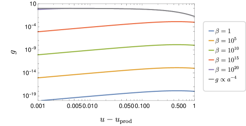
Figure 1: Peak locations of $g_{i}(a)$ for $u_{\mathrm{prod}}=-20$ (left), and the evolution of the contributions to $\tilde{\rho}_{\psi}$ by different $\tilde{\rho}_{i}$ for several values of $\beta_{i}$ (right).

After all contributions pass their maxima at $a=2^{2/3}a_{\rm{prod}}$, the ratio $g_{i}(a)/g_{1}(a)$ of the contributions from $\tilde{\rho}_{i}$ and $\tilde{\rho}_{1}$ to $\rho_{\psi}$ always decreases, since $\tilde{\rho}_{1}$ corresponds to the slowest decaying field. We can therefore use the ratios $g_{k}/g_{1}$ to discriminate relevant from irrelevant fields, in the indirect sense. We say that a field is indirectly irrelevant if

$$\mathcal{C}_{3}^{(k)}:\left.\frac{g_{k}(a)}{g_{1}(a)}\right|_{a=2^{2/3}a_{\rm{prod}}}<\varepsilon_{g}\,,$$ (22)

which allows discrimination between models in which some field contributions to $\rho_{\psi}$ become negligible very early.

Besides the conditions mentioned above, there is one additional way in which the value of $N$ is ambiguous. If there are multiple fields for which $\beta_{i}\,a_{\rm{prod}}^{2}>1/\varepsilon_{\beta}$ and they reach their maximum contribution to $\rho_{\psi}$ very early, their overall contribution to $\tilde{\rho}_{\psi}$ is

$$\sum_{i}g_{i}(a)=\left(\frac{a_{\rm{prod}}}{a}\right)^{4}\sum_{i}\tilde{\rho}_{i,p}\,,$$ (23)

which is indistinguishable from a single field with initial density $\sum_{i}\tilde{\rho}_{i,p}$ and a very large decay rate. We therefore impose an additional condition, which is that at most one field has a decay rate such that $\beta_{i}\,a_{\rm{prod}}^{2}>1/\varepsilon_{\beta}$. Since the largest decay rate is that of $i=N$, this condition can be expressed as

$$\mathcal{C}_{0}:\beta_{N-1}a_{\rm{prod}}^{2}<\varepsilon_{\beta}\,.$$ (24)

These conditions can be implemented as a prior in the Bayesian method described below, so that, for each $N$, we exclude the regions of the parameter space that contain at least one field that is both directly and indirectly irrelevant. Said differently, if either $\mathcal{C}_{0}$ is true, or if there exists a $k$ such that $(\mathcal{C}_{1}^{(k)}\lor\mathcal{C}_{2}^{(k)})\land\mathcal{C}_{3}^{(k)}$ is true, then we assign a null prior to the model. For the models studied below, we choose conservative conditions with $(\varepsilon_{\rho},\varepsilon_{\beta},\varepsilon_{g})=(10^{-25},2\times 10^{5},10^{-10})$.

IV.4 The Markov Chain Monte Carlo

We use a Markov Chain Monte Carlo (MCMC) Bayesian method to study how the data constrains the model parameters. We implement an adaptive Metropolis algorithm as described in Ref. haario:2001 , in which a fixed proposal distribution is used for some small number of steps at the beginning of the chain, after which the covariance matrix of all previously sampled points is used as the covariance matrix for a multivariate normal proposal distribution. This allows the chain to adapt to the vastly different variances along different dimensions.

We consider a prior comprised of bounded uniform distributions on the cosmological parameters $h_{0}$ and $\Omega_{\Lambda}$, and $M_{B}$, in the intervals in Table 1. The lower limit on $h_{0}$ and the upper limit on $\Omega_{\Lambda}$ are to ensure positivity of the energy densities.

Table 1: Prior ranges for $h_{0}$, $\Omega_{\Lambda}$ and $M_{B}$.

parameter	range
$h_{0}$	$[\sqrt{\alpha},1]$
$\Omega_{\Lambda}$	$[0,1-\alpha/h_{0}^{2}]$
$M_{B}$	$[-25,-15]$

The priors on the initial conditions and the decay rates are also uniform with bounds chosen to implement the relevance conditions defined in §IV.3.

V Numerical Analysis

We begin by presenting the results of the fit for a few cases of relatively low $N$ (1, 2 and 10) with $\Lambda$CDM as the baseline model. We first show the posterior distributions for the cosmological parameters $h_{0}$ and $\Omega_{\Lambda}$, together with $M_{B}$, which are common to all models. The 1D and 2D 68% CL and 95% CL distributions are shown in Fig. 2. Clearly, none of the models differ from $\Lambda$CDM in their predictions for $h_{0}$ and $M_{B}$, while predictions for $\Omega_{\Lambda}$ differ significantly. A large increase in $\Omega_{\Lambda}$ occurs for $N=1$, a case in which the only decaying field has to account for all the dark matter during the evolution. Nonzero decay rates produce low values of $\Omega_{\mathrm{D}M}$ unless the initial density for the field is high, which is incompatible with the early universe data. Therefore, there is more room for dark energy. As the number of fields increases, the decay rate of the slowest decaying field decreases, allowing for an overall increase in $\Omega_{\rm DM}$.

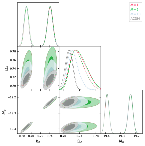
Figure 2: 1D and 2D 68% CL and 95% CL posterior distributions for $h_{0}$, $\Omega_{\Lambda}$ and $M_{B}$ for the $\Lambda$CDM and $N=1,2,10$ models. In the 1D posteriors, the solid lines are for $r_{d,l}$ and the dashed ones for $r_{d,e}$. These two values produce separate islands in the 2D contour plots, with lower $h_{0}$ and $M_{B}$ for $r_{d,e}$ than for $r_{d,l}$. This clearly shows how the discrepancies in $H_{0}$, $M_{B}$ and $r_{d}$ are related.

Regarding the model parameters (decay rates and initial densities), the results point to a slowly decaying field and a collection of fields decaying in the very early universe. In Fig. 3 we show the decay rate $\tilde{\Gamma}_{1}$ of the slowest decaying field. Note that by definition, a value of order unity is approximately the age of the Universe.

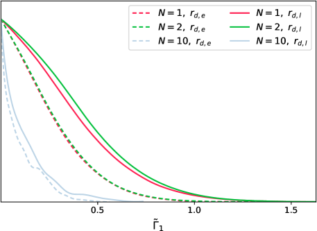
Figure 3: Decay rates of the slowest decaying field for $N=1,2,10$ and both values of $r_{d}$.

In the $N=2$ case, there is an additional decaying field besides the slowly decaying field of Fig. 3. The posterior distribution for its decay rate becomes flat at its maximum value, so that the field decays in the very early Universe. Thus, we conclude that with two fields, one has a decay rate close to zero, while the other has a vanishing lifetime. This explains why the results for $N=1$ and $N=2$ in Fig. 2 are so similar.

The posterior distributions for the parameters in the $N=10$ case show more structure, due to the imposition of the relevance conditions on the decay rates. Nevertheless, we decide not to include them here since Fig. 2 already shows that the model cannot affect $h_{0}$ significantly.

We now consider a large ensemble of fields and a simple parametrization for their initial densities and decay rates Desai:2019pvs :

$$\tilde{\Gamma}_{n}=\tilde{\Gamma}_{1}\left[1+(n-1)^{\delta}\Delta\right]^{\xi}\,,$$ (25a)

$$\tilde{\rho}_{n,\mathrm{prod}}=\tilde{\rho}_{1,\mathrm{prod}}\left[1+(n-1)^{\delta}\Delta\right]^{\zeta}\,.$$ (25b)

We choose $\delta=1$ and $\Delta=0.1$ and perform a similar analysis to the one presented above, for the cosmological parameters and $(\tilde{\Gamma}_{1},\tilde{\rho}_{1,\mathrm{prod}},\xi,\zeta)$. Here, the relevance conditions introduced in IV.3 must also be taken into account. They directly constrain the $\xi,\zeta$ parameter space for a given $N$. We choose $N=100$ as a compromise between computing time to solve the system of equations and a large enough number of fields that the decay times and initial densities are distributed smoothly between the slowest and the fastest decaying fields. The results are encapsulated in Fig. 4. In Fig. 5 we show a comparison of the relevant parameters with those obtained for the $\Lambda\mathrm{CDM}$ model. It is evident that this model does not address the Hubble tension in a more satisfactory way than the small $N$ models.

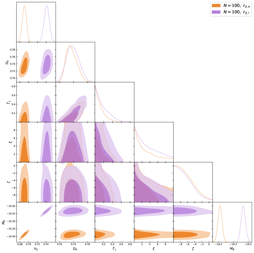
Figure 4: 1D and 2D posterior distributions for all free parameters of the $N=100$ model.

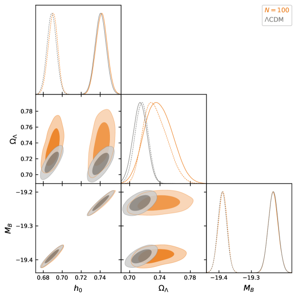
Figure 5: 1D and 2D posterior distributions for $h_{0}$, $\Omega_{\Lambda}$ and $M_{B}$ for $\Lambda$CDM and $N=100$. In the 1D posteriors, the solid lines are for $r_{d,l}$ and the dashed ones for $r_{d,e}$.

Finally, for completeness, in Fig. 6 we show the derived posterior distribution for the calculated values of $\Delta N_{\rm eff}$. We see that in all the cases the contribution to $\Delta N_{\rm eff}$ is comfortably below the bound given in Eq. (10). Note also that for $N=2$, the contribution to $\Delta N_{\rm eff}$ is consistent with the value reported in model 1 of Anchordoqui:2021gji .

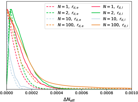
Figure 6: 1D posterior distributions for $\Delta N_{\rm eff}$ for $N=1,2,10,100$.

VI Conclusions

To address the Hubble tension, we examined dark sectors containing a large number of decaying degrees of freedom with no trivial dynamics, with a focus on decay processes that take place entirely among the dark constituents. We further restricted ourselves to ensembles in which CDM particles decay primarily to dark radiation in different epochs. We showed that the data favor stable dark matter particles and that a resolution of the $H_{0}$ tension with this type of dark matter ensemble is elusive.

In closing, we comment on some interesting extensions that could potentially evade our conclusion. Perhaps the most compelling of these are models in which decays to final states that include other relativistic massive particles occur. This allows for a dynamic equation of state. It was recently shown in Ref. Clark:2021hlo that the combination of such an $N=2$ model and an early period of dark energy domination which reduces the linear size of the sound horizon can ameliorate the $H_{0}$ tension to within the 95% CL. The early dark energy is modeled by a scalar field that behaves like a cosmological constant at high redshifts ($z>3000$) which then gets diluted at the same rate or faster than radiation as the universe expands Poulin:2018cxd . We anticipate that in principle, a similar reduction of the acoustic horizon may be obtained by enlarging the dark matter ensemble to allow for very short-lived constituents that decay into particles that are born relativistic but behave as CDM before recombination. Our conclusion may also be evaded in models characterized by an ensemble in which the CDM particles decay into self-interacting dark radiation (as in stepped fluids Aloni:2021eaq ), and models in which the ensemble couples to the dark energy sector through a quintessence field (as in string backgrounds with Standard Model fields confined on Neveu-Schwarz 5-branes Anchordoqui:2019amx ).

References

- (1) N. Aghanim et al. [Planck Collaboration], Planck 2018 results. VI. Cosmological parameters, Astron. Astrophys. 641, A6 (2020) doi:10.1051/0004-6361/201833910 [arXiv:1807.06209 [astro-ph.CO]].
- (2) A. G. Riess, S. Casertano, W. Yuan, J. B. Bowers, L. Macri, J. C. Zinn and D. Scolnic, Cosmic distances calibrated to 1% precision with Gaia EDR3 parallaxes and Hubble Space Telescope photometry of 75 Milky Way cepheids confirm tension with CDM, Astrophys. J. Lett. 908, no.1, L6 (2021) doi:10.3847/2041-8213/abdbaf [arXiv:2012.08534 [astro-ph.CO]].
- (3) E. Di Valentino, L. A. Anchordoqui, O. Akarsu, Y. Ali-Haimoud, L. Amendola, N. Arendse, M. Asgari, M. Ballardini, S. Basilakos and E. Battistelli, et al. Snowmass2021 - Letter of interest cosmology intertwined II: The hubble constant tension, Astropart. Phys. 131, 102605 (2021) doi:10.1016/j.astropartphys.2021.102605 [arXiv:2008.11284 [astro-ph.CO]].
- (4) L. Verde, T. Treu and A. G. Riess, Tensions between the early and the late Universe, Nature Astron. 3, 891 doi:10.1038/s41550-019-0902-0 [arXiv:1907.10625 [astro-ph.CO]].
- (5) E. Di Valentino, L. A. Anchordoqui, Ö. Akarsu, Y. Ali-Haimoud, L. Amendola, N. Arendse, M. Asgari, M. Ballardini, S. Basilakos and E. Battistelli, et al. Cosmology intertwined III: and , Astropart. Phys. 131, 102604 (2021) doi:10.1016/j.astropartphys.2021.102604 [arXiv:2008.11285 [astro-ph.CO]].
- (6) E. Di Valentino, O. Mena, S. Pan, L. Visinelli, W. Yang, A. Melchiorri, D. F. Mota, A. G. Riess and J. Silk, In the realm of the Hubble tension—a review of solutions, Class. Quant. Grav. 38, no.15, 153001 (2021) doi:10.1088/1361-6382/ac086d [arXiv:2103.01183 [astro-ph.CO]].
- (7) N. Schöneberg, G. F. Abellán, A. P. Sánchez, S. J. Witte, c. V. Poulin and J. Lesgourgues, The Olympics: A fair ranking of proposed models, [arXiv:2107.10291 [astro-ph.CO]].
- (8) L. A. Anchordoqui, E. Di Valentino, S. Pan and W. Yang, Dissecting the and tensions with Planck + BAO + supernova type Ia in multi-parameter cosmologies, JHEAp 32, 28-64 (2021) doi:10.1016/j.jheap.2021.08.001 [arXiv:2107.13932 [astro-ph.CO]].
- (9) J. L. Menestrina and R. J. Scherrer, Dark radiation from particle decays during big bang nucleosynthesis, Phys. Rev. D 85, 047301 (2012) doi:10.1103/PhysRevD.85.047301 [arXiv:1111.0605 [astro-ph.CO]].
- (10) D. Hooper, F. S. Queiroz and N. Y. Gnedin, Non-thermal dark matter mimicking an additional neutrino species in the early universe, Phys. Rev. D 85, 063513 (2012) doi:10.1103/PhysRevD.85.063513 [arXiv:1111.6599 [astro-ph.CO]].
- (11) M. C. Gonzalez-Garcia, V. Niro and J. Salvado, Dark radiation and decaying matter, JHEP 04, 052 (2013) doi:10.1007/JHEP04(2013)052 [arXiv:1212.1472 [hep-ph]].
- (12) Z. Berezhiani, A. D. Dolgov and I. I. Tkachev, Reconciling Planck results with low redshift astronomical measurements, Phys. Rev. D 92, no.6, 061303 (2015) doi:10.1103/PhysRevD.92.061303 [arXiv:1505.03644 [astro-ph.CO]].
- (13) K. Vattis, S. M. Koushiappas and A. Loeb, Dark matter decaying in the late Universe can relieve the tension, Phys. Rev. D 99, no.12, 121302 (2019) doi:10.1103/PhysRevD.99.121302 [arXiv:1903.06220 [astro-ph.CO]].
- (14) K. Enqvist, S. Nadathur, T. Sekiguchi and T. Takahashi, Decaying dark matter and the tension in , JCAP 09, 067 (2015) doi:10.1088/1475-7516/2015/09/067 [arXiv:1505.05511 [astro-ph.CO]].
- (15) G. F. Abellan, R. Murgia, V. Poulin and J. Lavalle, Hints for decaying dark matter from measurements, [arXiv:2008.09615 [astro-ph.CO]].
- (16) G. F. Abellán, R. Murgia and V. Poulin, Linear cosmological constraints on two-body decaying dark matter scenarios and the S8 tension, Phys. Rev. D 104, no.12, 12 (2021) doi:10.1103/PhysRevD.104.123533 [arXiv:2102.12498 [astro-ph.CO]].
- (17) L. A. Anchordoqui, V. Barger, H. Goldberg, X. Huang, D. Marfatia, L. H. M. da Silva and T. J. Weiler, IceCube neutrinos, decaying dark matter, and the Hubble constant, Phys. Rev. D 92, no.6, 061301 (2015) [erratum: Phys. Rev. D 94, no.6, 069901 (2016)] doi:10.1103/PhysRevD.94.069901 [arXiv:1506.08788 [hep-ph]].
- (18) L. A. Anchordoqui, V. Barger, D. Marfatia, M. H. Reno and T. J. Weiler, Oscillations of sterile neutrinos from dark matter decay eliminates the IceCube-Fermi tension, Phys. Rev. D 103, no.7, 075022 (2021) doi:10.1103/PhysRevD.103.075022 [arXiv:2101.09559 [astro-ph.HE]].
- (19) A. Chudaykin, D. Gorbunov and I. Tkachev, Dark matter component decaying after recombination: Lensing constraints with Planck data, Phys. Rev. D 94, 023528 (2016) doi:10.1103/PhysRevD.94.023528 [arXiv:1602.08121 [astro-ph.CO]].
- (20) V. Poulin, P. D. Serpico and J. Lesgourgues, A fresh look at linear cosmological constraints on a decaying dark matter component, JCAP 08, 036 (2016) doi:10.1088/1475-7516/2016/08/036 [arXiv:1606.02073 [astro-ph.CO]].
- (21) S. J. Clark, K. Vattis and S. M. Koushiappas, Cosmological constraints on late-universe decaying dark matter as a solution to the tension, Phys. Rev. D 103, no.4, 043014 (2021) doi:10.1103/PhysRevD.103.043014 [arXiv:2006.03678 [astro-ph.CO]].
- (22) A. Chudaykin, D. Gorbunov and I. Tkachev, Dark matter component decaying after recombination: Sensitivity to baryon acoustic oscillation and redshift space distortion probes, Phys. Rev. D 97, no.8, 083508 (2018) doi:10.1103/PhysRevD.97.083508 [arXiv:1711.06738 [astro-ph.CO]].
- (23) A. Nygaard, T. Tram and S. Hannestad, Updated constraints on decaying cold dark matter, JCAP 05, 017 (2021) doi:10.1088/1475-7516/2021/05/017 [arXiv:2011.01632 [astro-ph.CO]].
- (24) L. A. Anchordoqui, Decaying dark matter, the tension, and the lithium problem, Phys. Rev. D 103, no.3, 035025 (2021) doi:10.1103/PhysRevD.103.035025 [arXiv:2010.09715 [hep-ph]].
- (25) K. R. Dienes and B. Thomas, Dynamical dark matter I: theoretical overview, Phys. Rev. D 85, 083523 (2012) doi:10.1103/PhysRevD.85.083523 [arXiv:1106.4546 [hep-ph]].
- (26) D. M. Scolnic et al., The complete light-curve sample of spectroscopically confirmed SNe Ia from Pan-STARRS1 and cosmological constraints from the combined Pantheon sample, Astrophys. J. 859, no.2, 101 (2018) doi:10.3847/1538-4357/aab9bb [arXiv:1710.00845 [astro-ph.CO]].
- (27) A. Desai, K. R. Dienes and B. Thomas, Constraining dark-matter ensembles with supernova data, Phys. Rev. D 101, no.3, 035031 (2020) doi:10.1103/PhysRevD.101.035031 [arXiv:1909.07981 [astro-ph.CO]].
- (28) P. A. Zyla et al. [Particle Data Group], Review of Particle Physics, PTEP 2020, no.8, 083C01 (2020) doi:10.1093/ptep/ptaa104
- (29) R. J. Cooke, M. Pettini, K. M. Nollett and R. Jorgenson, The primordial deuterium abundance of the most metal-poor damped Ly system, Astrophys. J. 830, no.2, 148 (2016) doi:10.3847/0004-637X/830/2/148 [arXiv:1607.03900 [astro-ph.CO]].
- (30) V. Mossa et al., The baryon density of the Universe from an improved rate of deuterium burning, Nature 587, no.7833, 210-213 (2020) doi:10.1038/s41586-020-2878-4
- (31) G. Steigman, D. N. Schramm and J. E. Gunn, Cosmological limits to the number of massive leptons, Phys. Lett. B 66, 202-204 (1977) doi:10.1016/0370-2693(77)90176-9
- (32) G. Mangano, G. Miele, S. Pastor, T. Pinto, O. Pisanti and P. D. Serpico, Relic neutrino decoupling including flavor oscillations, Nucl. Phys. B 729, 221 (2005) doi:10.1016/j.nuclphysb.2005.09.041 [hep-ph/0506164].
- (33) N. Arendse, R. J. Wojtak, A. Agnello, G. C. F. Chen, C. D. Fassnacht, D. Sluse, S. Hilbert, M. Millon, V. Bonvin and K. C. Wong, et al. Cosmic dissonance: are new physics or systematics behind a short sound horizon?, Astron. Astrophys. 639, A57 (2020) doi:10.1051/0004-6361/201936720 [arXiv:1909.07986 [astro-ph.CO]].
- (34) R. G. Cai, Z. K. Guo, S. J. Wang, W. W. Yu and Y. Zhou, A no-go guide for the Hubble tension, Phys. Rev. D 105, no.2, L021301 (2022) doi:10.1103/PhysRevD.105.L021301 [arXiv:2107.13286 [astro-ph.CO]].
- (35) R. Jimenez and A. Loeb, Constraining cosmological parameters based on relative galaxy ages, Astrophys. J. 573, 37-42 (2002) doi:10.1086/340549 [arXiv:astro-ph/0106145 [astro-ph]].
- (36) G. Bruzual and S. Charlot, Stellar population synthesis at the resolution of 2003, Mon. Not. Roy. Astron. Soc. 344, 1000 (2003) doi:10.1046/j.1365-8711.2003.06897.x [arXiv:astro-ph/0309134 [astro-ph]].
- (37) R. Jimenez, L. Verde, T. Treu and D. Stern, G. Bruzual and S. Charlot, Constraints on the equation of state of dark energy and the Hubble constant from stellar ages and the CMB, Astrophys. J. 593, 622-629 (2003) doi:10.1086/376595 [arXiv:astro-ph/0302560 [astro-ph]].
- (38) J. Simon, L. Verde and R. Jimenez, G. Bruzual and S. Charlot, Constraints on the redshift dependence of the dark energy potential, Phys. Rev. D 71, 123001 (2005) doi:10.1103/PhysRevD.71.123001 [arXiv:astro-ph/0412269 [astro-ph]].
- (39) D. Stern, R. Jimenez, L. Verde, M. Kamionkowski and S. A. Stanford, G. Bruzual and S. Charlot, Cosmic Chronometers: Constraining the Equation of State of Dark Energy. I: H(z) Measurements, JCAP 02, 008 (2010) doi:10.1088/1475-7516/2010/02/008 [arXiv:0907.3149 [astro-ph.CO]].
- (40) M. Moresco et al., Improved constraints on the expansion rate of the Universe up to from the spectroscopic evolution of cosmic chronometers, JCAP 08, 006 (2012) doi:10.1088/1475-7516/2012/08/006 [arXiv:1201.3609 [astro-ph.CO]].
- (41) C. Zhang, H. Zhang, S. Yuan, T. J. Zhang and Y. C. Sun, G. Bruzual and S. Charlot, Four new observational data from luminous red galaxies in the Sloan Digital Sky Survey data release seven, Res. Astron. Astrophys. 14, no.10, 1221-1233 (2014) doi:10.1088/1674-4527/14/10/002 [arXiv:1207.4541 [astro-ph.CO]].
- (42) M. Moresco, G. Bruzual and S. Charlot, Raising the bar: new constraints on the Hubble parameter with cosmic chronometers at 2, Mon. Not. Roy. Astron. Soc. 450, no.1, L16-L20 (2015) doi:10.1093/mnrasl/slv037 [arXiv:1503.01116 [astro-ph.CO]].
- (43) M. Moresco, L. Pozzetti, A. Cimatti, R. Jimenez, C. Maraston, L. Verde, D. Thomas, A. Citro, R. Tojeiro and D. Wilkinson, G. Bruzual and S. Charlot, A 6% measurement of the Hubble parameter at : direct evidence of the epoch of cosmic re-acceleration, JCAP 05, 014 (2016) doi:10.1088/1475-7516/2016/05/014 [arXiv:1601.01701 [astro-ph.CO]].
- (44) F. Beutler, C. Blake, M. Colless, D. H. Jones, L. Staveley-Smith, L. Campbell, Q. Parker, W. Saunders and F. Watson, The 6dF Galaxy Survey: baryon acoustic oscillations and the local Hubble constant, Mon. Not. Roy. Astron. Soc. 416, 3017-3032 (2011) doi:10.1111/j.1365-2966.2011.19250.x [arXiv:1106.3366 [astro-ph.CO]].
- (45) A. J. Ross, L. Samushia, C. Howlett, W. J. Percival, A. Burden and M. Manera, The clustering of the SDSS DR7 main galaxy sample – I. A 4 per cent distance measure at , Mon. Not. Roy. Astron. Soc. 449, no.1, 835-847 (2015) doi:10.1093/mnras/stv154 [arXiv:1409.3242 [astro-ph.CO]].
- (46) Y. Wang et al. [BOSS Collaboration], The clustering of galaxies in the completed SDSS-III Baryon Oscillation Spectroscopic Survey: tomographic BAO analysis of DR12 combined sample in configuration space, Mon. Not. Roy. Astron. Soc. 469, no.3, 3762-3774 (2017) doi:10.1093/mnras/stx1090 [arXiv:1607.03154 [astro-ph.CO]].
- (47) M. Ata et al., The clustering of the SDSS-IV extended Baryon Oscillation Spectroscopic Survey DR14 quasar sample: first measurement of baryon acoustic oscillations between redshift 0.8 and 2.2, Mon. Not. Roy. Astron. Soc. 473, no.4, 4773-4794 (2018) doi:10.1093/mnras/stx2630 [arXiv:1705.06373 [astro-ph.CO]].
- (48) V. de Sainte Agathe et al., Baryon acoustic oscillations at from the correlations of Ly absorption in eBOSS DR14, Astron. Astrophys. 629, A85 (2019) doi:10.1051/0004-6361/201935638 [arXiv:1904.03400 [astro-ph.CO]].
- (49) M. Blomqvist et al., Baryon acoustic oscillations from the cross-correlation of Ly absorption and quasars in eBOSS DR14, Astron. Astrophys. 629, A86 (2019) doi:10.1051/0004-6361/201935641 [arXiv:1904.03430 [astro-ph.CO]].
- (50) J. E. Bautista et al., The completed SDSS-IV extended Baryon Oscillation Spectroscopic Survey: measurement of the BAO and growth rate of structure of the luminous red galaxy sample from the anisotropic correlation function between redshifts 0.6 and 1, Mon. Not. Roy. Astron. Soc. 500, no.1, 736-762 (2020) doi:10.1093/mnras/staa2800 [arXiv:2007.08993 [astro-ph.CO]].
- (51) H. Gil-Marin et al., The completed SDSS-IV extended Baryon Oscillation Spectroscopic Survey: measurement of the BAO and growth rate of structure of the luminous red galaxy sample from the anisotropic power spectrum between redshifts 0.6 and 1.0, Mon. Not. Roy. Astron. Soc. 498, no.2, 2492-2531 (2020) doi:10.1093/mnras/staa2455 [arXiv:2007.08994 [astro-ph.CO]].
- (52) A. de Mattia et al., The completed SDSS-IV extended Baryon Oscillation Spectroscopic Survey: measurement of the BAO and growth rate of structure of the emission line galaxy sample from the anisotropic power spectrum between redshift 0.6 and 1.1, Mon. Not. Roy. Astron. Soc. 501, no.4, 5616-5645 (2021) doi:10.1093/mnras/staa3891 [arXiv:2007.09008 [astro-ph.CO]].
- (53) A. Tamone et al., The completed SDSS-IV extended Baryon Oscillation Spectroscopic Survey: growth rate of structure measurement from anisotropic clustering analysis in configuration space between redshift 0.6 and 1.1 for the emission line galaxy sample, Mon. Not. Roy. Astron. Soc. 499, no.4, 5527-5546 (2020) doi:10.1093/mnras/staa3050 [arXiv:2007.09009 [astro-ph.CO]].
- (54) R. Neveux et al., The completed SDSS-IV extended Baryon Oscillation Spectroscopic Survey: BAO and RSD measurements from the anisotropic power spectrum of the quasar sample between redshift 0.8 and 2.2, Mon. Not. Roy. Astron. Soc. 499, no.1, 210-229 (2020) doi:10.1093/mnras/staa2780 [arXiv:2007.08999 [astro-ph.CO]].
- (55) J. Hou et al., The completed SDSS-IV extended Baryon Oscillation Spectroscopic Survey: BAO and RSD measurements from anisotropic clustering analysis of the quasar sample in configuration space between redshift 0.8 and 2.2, Mon. Not. Roy. Astron. Soc. 500, no.1, 1201-1221 (2020) doi:10.1093/mnras/staa3234 [arXiv:2007.08998 [astro-ph.CO]].
- (56) H. du Mas des Bourboux et al., The completed SDSS-IV extended Baryon Oscillation Spectroscopic Survey: baryon acoustic oscillations with Ly forests, Astrophys. J. 901, no.2, 153 (2020) doi:10.3847/1538-4357/abb085 [arXiv:2007.08995 [astro-ph.CO]].
- (57) T. M. C. Abbott et al. [DES Collaboration], Dark Energy Survey year 3 results: A 2.7% measurement of baryon acoustic oscillation distance scale at redshift 0.835, [arXiv:2107.04646 [astro-ph.CO]].
- (58) A. G. Riess et al., A comprehensive measurement of the local value of the Hubble constant with 1 km/s/Mpc uncertainty from the Hubble Space Telescope and the SH0ES team, [arXiv:2112.04510 [astro-ph.CO]].
- (59) H. Haario, E. Saksman and J. Tamminen An adaptive metropolis algorithm, Bernoulli 7, no.2, 223 (2001) doi:10.2307/3318737
- (60) S. J. Clark, K. Vattis, J. Fan and S. M. Koushiappas, The and tensions necessitate early and late time changes to CDM [arXiv:2110.09562 [astro-ph.CO]].
- (61) V. Poulin, T. L. Smith, T. Karwal and M. Kamionkowski, Early dark energy can resolve the Hubble tension, Phys. Rev. Lett. 122, no.22, 221301 (2019) doi:10.1103/PhysRevLett.122.221301 [arXiv:1811.04083 [astro-ph.CO]].
- (62) D. Aloni, A. Berlin, M. Joseph, M. Schmaltz and N. Weiner, A step in understanding the Hubble tension, [arXiv:2111.00014 [astro-ph.CO]].
- (63) L. A. Anchordoqui, I. Antoniadis, D. Lüst, J. F. Soriano and T. R. Taylor, tension and the String Swampland, Phys. Rev. D 101, 083532 (2020) doi:10.1103/PhysRevD.101.083532 [arXiv:1912.00242 [hep-th]].