How many Observations are Enough?
Knowledge Distillation for Trajectory Forecasting - Supplementary Material

1 Time lags

	$\nabla x_{t}=1$	$\nabla x_{t}=2$	$\nabla x_{t}=3$
Input	($x_{7},x_{8}$)	($x_{6},x_{8}$)	($x_{5},x_{8}$)
STT	0.73 / 1.44	0.80 / 1.53	0.88 / 1.63
DTO	0.64 / 1.27	0.66 / 1.32	0.69 / 1.37

Table 1: On the SDD, an analysis of increasing time-lags $\nabla x_{t}$ with a fixed number of observed time steps (only two).

We also investigate how our method performs when increasing the lag between the two observation used for prediction. As highlighted in Tab. 1, the procedure we set up yields robust performance even in this setting.

2 On the “length-shift problem” – additional considerations

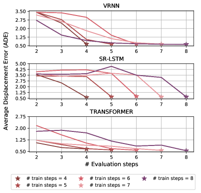
Figure 1: For different architectures (Variational RNN [4], SR-LSTM [14] and our STT), the performance trends when altering the number of observation time steps at evaluation time (ETH).

As outlined in Sec. 5.5, trajectory prediction models show remarkable performance when evaluated according to the standard protocol, viz., $8$ observation time steps and $12$ prediction time steps. Nevertheless, we argue that their predictions overly bind to the data used at training time. To prove our intuition, we thoroughly investigate how models behave when the number of input time steps changes at evaluation time, which we define as “length-shift problem”.

As shown in Fig. 1, this behaviour is a common trait among different models: more specifically, we report the ADE metric for different categories of predictors (generative [4], LSTM-based [14], attention-based) and observation-prediction splits ($8$–$12$, $7$–$12$, etc.). As expected, the optimum always occurs when train/test conditions met; on the contrary, altering the amount of input information (even slightly, i.e., removing a single time step) produces detrimental effects and delivers unacceptable inference errors. This behaviour could limit the usage of these models when there is no perfect match between train/test conditions.

Dataset	Training strategy	obs=2	obs=3	obs=4	obs=5	obs=6	obs=7	obs=8
SDD	From scratch	0.73/1.44	0.67/1.31	0.65/1.30	0.65/1.29	0.64/1.29	0.65/1.32	0.63/1.26
	Variable observations	0.92/1.78	0.95/1.75	0.97/1.75	0.89/1.63	0.82/1.55	0.81/1.54	0.83/1.56
	Past generation	0.85/1.58	0.76/1.45	0.73/1.42	0.74/1.45	0.71/1.39	0.67/1.35	-
	Distilling the Observations	0.64/1.27	0.64/1.27	0.64/1.28	0.64/1.28	0.63/1.26	0.62/1.22	0.63/1.27

Table 2: Comparison (ADE/FDE) between different training strategies on the Stanford Drone Dataset; all methods are trained and tested on the same number of time steps, reported in the header. Best results are in bold. The distillation teacher is in underlined italic.

Addressing the length-shift problem on the Stanford Drone Dataset. We also report our results using different training strategies on the Stanford Drone Dataset (Tab. 2). These results are similar to what has been observed on ETH/UCY and Lyft datasets. Training from scratch gives unsatisfactory results: the student is not able to observe enough information about agents’ motion history. Training with a variable number of observations makes our model invariant to the amount of information it is fed with, but it delivers overly high errors. Generating missing observations introduces too much noise to obtain reliable predictions. As reported in the main paper, DTO appears the most promising strategy, being able to exploit enough past information even when the number of observations is limited.

3 Spatial masking

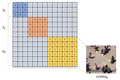
Figure 2: Example of a batch mask for the STT spatial attention. Before the softmax layer, logits corresponding to $0$ values are masked and set to $-\infty$. This way, agents are allowed to attend only on the neighbouring agents in the same scene (e.g. scene $k$) at the given time step.

Our Spatio-Temporal solution (STT) relies on a single transformer-based architecture with shared parameters. Since batches are composed of randomly sampled scenes, performing a plain spatial self-attention without further solutions would result in attending on agents that appear in different scenes. To prevent attending on wrong agents, we build a dedicated spatial attention mask.

As done in [7, 9, 14, 13], we represent the pedestrian space as an undirected graph. In doing so, the adjacency matrix describes spatial relationships occurring among different nodes (agents). We employ a distance-based adjacency matrix where, in order to focus only on the neighbourhood, we preserve (i.e., set to 1) the edges that are associated to distances smaller than a given threshold $d$. Moreover, as shown in Fig. 2, we cluster adjacency matrices of different scenes in batches by devising a block irregular matrix: this matrix is built by aligning several adjacency matrices on the main diagonal and by setting to $0$ the remaining values.

By employing this matrix as a mask applied to the logits before the softmax operation, we are able to restrict the attention scope only to agents that: i) share the same scene and time steps; ii) are spatially close to each other. In our implementation, we set to $-\infty$ all the attention logits corresponding to $0$-values in the mask.

4 Datasets preprocessing

Frame-rate. Following the ETH/UCY setting proposed in [1, 6, 10], we employ a sampling rate of 2.5 FPS. By sampling agents’ positions every $0.4s$, employing $8$ frames of observation and $12$ frames of prediction corresponds to observe the trajectories for $3.2~{}s$ and predicting their future development in the next $4.2~{}s$. We use the same frame also for both Stanford Drone and Lyft datasets.

Data preparation. Several previous works [1, 6, 9, 2] represent input trajectories as a series of relative displacements: namely, each absolute position $\mathbf{x}_{t}$ is transformed in a couple of displacements $(\Delta x_{t},\Delta y_{t})$ w.r.t. the previous position $\mathbf{x}_{t-1}$. Differently, [14] proposes to preserve absolute positions and normalize them by subtracting the last observation: this procedure, referred to as Nabs, seems to grant higher benefits. We opt for this solution (as in [13]).

ETH/UCY issues. Recent works [14, 11] brought up several issues affecting the ETH/UCY dataset. [14] points out that the original video used to obtain the labelled trajectories for the ETH scenario is accelerated, thus strongly affecting the resulting motion patterns: when sampling at a fixed rate, the trajectories of this scenario present higher speeds than the ones captured in the remaining scenes. The authors mitigate this issue by treating $0.4$ s as $6$ frames instead of the original $10$ frames. To ensure a fair comparison [14, 13], we choose to adopt the same correction.

In addition, [11] shows that Hotel scene mostly contains trajectories that are orthogonal to the ones contained in the other four scenarios. This peculiarity could prevent the model from learning useful environmental priors. To overcome this issue, we follow [14, 13] and employ data augmentation by applying a random rotation to each position inside each mini-batch.

5 Implementation details

Teacher. We initialize the weights of our architecture according to [5]. All teacher networks are trained for $1000$ epochs using Adam [8] as optimizer.

For ETH/UCY, our Spatio-Temporal Transformer employs two layers for each encoder and decoder stack. We use internal embeddings of size $d_{\text{model}}=64$ and set the dimension $d_{\text{ff}}$ of the position-wise feed-forward inner layer to $128$. We employ $8$ attention heads for each temporal and spatial attention and set the size of queries, keys and values to $d_{\text{k}}=d_{\text{v}}=d_{\text{model}}/8=8$: reducing the dimension of each head allows to obtain a similar computation cost to a single-head attention with “full” dimensionality [12]. We use a batch size of $16$ and a learning rate of $10^{-4}$.

For SDD, our Spatio-Temporal Transformer employs a single layer for each stack. We use internal embeddings of size $d_{\text{model}}=32$ and set the dimension $d_{\text{ff}}$ of the position-wise feed-forward inner layer to $128$. We employ $8$ attention heads for each temporal and spatial attention and, as reported above, obtain the size of queries, keys and values by dividing $d_{\text{model}}$ by the number of heads. We use a batch size of $32$ and a learning rate of $5\cdot 10^{-4}$.

For Lyft, our Spatio-Temporal Transformer employs a single layer for each stack. We use internal embeddings of size $d_{\text{model}}=32$ and set the dimension $d_{\text{ff}}$ of the position-wise feed-forward inner layer to $128$. We employ $8$ attention heads for each temporal and spatial attention and, as said above, obtain the size of queries, keys and values by dividing $d_{\text{model}}$ by the number of heads. We use a batch size of $32$ and a learning rate of $5\cdot 10^{-5}$.

Distillation. Regarding the student initialization, we empirically found more beneficial to inherit the teacher weights rather starting from scratch. We believe that starting from a solid parametrization eases the student effort: this way, the student can just adjust the previously learned weights while preserving as much knowledge as possible. In contrast, we observe that learning weights from scratch represents an overly detrimental situation: the student rarely approaches the results of its teacher.

Furthermore, we set our teacher network in training mode during distillation. In this way, the statistics of the different normalization layers are computed on a batch basis: as reported in [3], this grants more accurate teacher supervision.

References

- [1] Alexandre Alahi, Kratarth Goel, Vignesh Ramanathan, Alexandre Robicquet, Li Fei-Fei, and Silvio Savarese. Social lstm: Human trajectory prediction in crowded spaces. In Proc. of the IEEE/CVF Conference on Computer Vision and Pattern Recognition (CVPR), 2016.
- [2] Javad Amirian, Jean-Bernard Hayet, and Julien Pettré. Social ways: Learning multi-modal distributions of pedestrian trajectories with gans. In Proc. of the IEEE/CVF Conference on Computer Vision and Pattern Recognition Workshops, 2019.
- [3] Hessam Bagherinezhad, Maxwell Horton, Mohammad Rastegari, and Ali Farhadi. Label refinery: Improving imagenet classification through label progression, 2018.
- [4] Junyoung Chung, Kyle Kastner, Laurent Dinh, Kratarth Goel, Aaron C Courville, and Yoshua Bengio. A recurrent latent variable model for sequential data. In Proc. of Advances in Neural Information Processing Systems (NeurIPS), 2015.
- [5] Xavier Glorot and Yoshua Bengio. Understanding the difficulty of training deep feedforward neural networks. In Proc. of the Int’l Conference on Artificial Intelligence and Statistics (AISTATS), 2010.
- [6] Agrim Gupta, Justin Johnson, Li Fei-Fei, Silvio Savarese, and Alexandre Alahi. Social GAN: Socially acceptable trajectories with generative adversarial networks. In Proc. of the IEEE/CVF Conference on Computer Vision and Pattern Recognition (CVPR), 2018.
- [7] Yingfan Huang, Huikun Bi, Zhaoxin Li, Tianlu Mao, and Zhaoqi Wang. Stgat: Modeling spatial-temporal interactions for human trajectory prediction. In Proc. of the IEEE/CVF International Conference on Computer Vision (ICCV), 2019.
- [8] Diederik P. Kingma and Jimmy Ba. Adam: A method for stochastic optimization. In Proc. of the International Conference on Learning Representations (ICLR), 2015.
- [9] Vineet Kosaraju, Amir Sadeghian, Roberto Martín-Martín, Ian Reid, Hamid Rezatofighi, and Silvio Savarese. Social-bigat: Multimodal trajectory forecasting using bicycle-gan and graph attention networks. In Proc. of Advances in Neural Information Processing Systems (NeurIPS), 2019.
- [10] Stefano Pellegrini, Andreas Ess, Konrad Schindler, and Luc Van Gool. You’ll never walk alone: Modeling social behavior for multi-target tracking. In Proc. of the IEEE/CVF International Conference on Computer Vision (ICCV), 2009.
- [11] C. Schöller, V. Aravantinos, F. Lay, and A. Knoll. What the constant velocity model can teach us about pedestrian motion prediction. Proc. of the IEEE international Conference on Robotics and Automation (ICRA), 2020.
- [12] Ashish Vaswani, Noam Shazeer, Niki Parmar, Jakob Uszkoreit, Llion Jones, Aidan N Gomez, Łukasz Kaiser, and Illia Polosukhin. Attention is all you need. In Proc. of Advances in Neural Information Processing Systems (NeurIPS), 2017.
- [13] Cunjun Yu, Xiao Ma, Jiawei Ren, Haiyu Zhao, and Shuai Yi. Spatio-temporal graph transformer networks for pedestrian trajectory prediction. In Proc. of the European Conference on Computer Vision (ECCV), 2020.
- [14] Pu Zhang, Wanli Ouyang, Pengfei Zhang, Jianru Xue, and Nanning Zheng. Sr-lstm: State refinement for lstm towards pedestrian trajectory prediction. In Proc. of the IEEE/CVF Conference on Computer Vision and Pattern Recognition (CVPR), 2019.