Relativistic second-order dissipative spin hydrodynamics from the method of moments

Abstract

We derive relativistic second-order dissipative fluid-dynamical equations of motion for massive spin-1/2 particles from kinetic theory using the method of moments. Besides the usual conservation laws for charge, energy, and momentum, such a theory of relativistic dissipative spin hydrodynamics features an equation of motion for the rank-3 spin tensor, which follows from the conservation of total angular momentum. Extending the conventional method of moments for spin-0 particles, we expand the spin-dependent distribution function near local equilibrium in terms of moments of the momentum and spin variables. We work to next-to-leading order in the Planck constant $\hbar$. As shown in previous work, at this order in $\hbar$ the Boltzmann equation for spin-1/2 particles features a nonlocal collision term. From the Boltzmann equation, we then obtain an infinite set of equations of motion for the irreducible moments of the deviation of the single-particle distribution function from local equilibrium. In order to close this system of moment equations, a truncation procedure is needed. We employ the “14+24-moment approximation”, where “14” corresponds to the components of the charge current and the energy-momentum tensor and “24” to the components of the spin tensor, which completes the derivation of the equations of motion of second-order dissipative spin hydrodynamics. For applications to heavy-ion phenomenology, we also determine dissipative corrections to the Pauli-Lubanski vector.

I Introduction

The derivation of a theory of relativistic hydrodynamics when spin degrees of freedom are dynamical variables coupled to the fluid, often referred to as “relativistic spin hydrodynamics”, has recently attracted a lot of attention Florkowski et al. (2018a, b); Hidaka et al. (2018); Florkowski et al. (2018c); Weickgenannt et al. (2019); Bhadury et al. (2021a); Weickgenannt et al. (2021a); Shi et al. (2021); Speranza and Weickgenannt (2021); Bhadury et al. (2021b); Singh et al. (2021); Bhadury et al. (2021c); Peng et al. (2021); Sheng et al. (2021, 2022); Hu (2021, 2022); Fang et al. (2022); Wang (2022); Montenegro and Torrieri (2019, 2020); Gallegos et al. (2021); Hattori et al. (2019); Fukushima and Pu (2021); Li et al. (2021); She et al. (2021); Wang et al. (2021a, b); Hongo et al. (2021). One of the main motivations to develop such a theory comes from the physics of the quark-gluon plasma (QGP) created in nuclear collisions. In this case, the vorticity of the hot and dense matter triggers hadron spin polarization in the final state Liang and Wang (2005); Voloshin (2004); Betz et al. (2007); Becattini et al. (2008). This mechanism resembles the time-honored Barnett effect Barnett (1935), which shows the interplay between a classical property of the system, the rotation, with the spin, which is a quantum property of matter. Experimental evidence of these phenomena comes from the analysis carried out in Refs. Adamczyk et al. (2017); Adam et al. (2018); Acharya et al. (2020); Mohanty et al. (2021), where it was shown that hadrons emitted in noncentral nuclear collisions are indeed spin-polarized. Theoretical models have successfully managed to describe the global-polarization data (i.e., the polarization along the direction of angular momentum of the collision) Becattini et al. (2008); Becattini et al. (2013a, b); Becattini et al. (2015, 2017); Karpenko and Becattini (2017); Pang et al. (2016); Xie et al. (2017). However, the explanation of the longitudinal-polarization data (i.e., the polarization along the beam direction) is still an open question Becattini and Karpenko (2018); Becattini and Lisa (2020); Florkowski et al. (2019a, b); Zhang et al. (2019); Becattini et al. (2019a); Xia et al. (2019); Wu et al. (2019); Sun and Ko (2019); Liu et al. (2020); Florkowski et al. (2022), see also important recent developments in Refs. Liu and Yin (2021); Fu et al. (2021); Becattini et al. (2021a, b). Since the spacetime evolution of the QGP is very accurately described by relativistic hydrodynamics Heinz and Snellings (2013); Florkowski et al. (2018d), it is natural to extend conventional relativistic hydrodynamics to incorporate the dynamics of spin. This novel theory, besides being of fundamental interest by itself as it connects quantum properties of matter with hydrodynamics, may provide an important tool towards a deeper understanding of relativistic strong-interaction matter under extreme conditions.

The basic idea of relativistic spin hydrodynamics, as put forward in Ref. Florkowski et al. (2018a), is that, in addition to the usual hydrodynamic quantities such as the energy-momentum tensor, one introduces the rank-3 spin tensor and studies its evolution using additional equations of motion constructed from the conservation of the total angular momentum of the system. Over the past few years, different methods to derive relativistic spin hydrodynamics have been applied: kinetic theory Florkowski et al. (2018a, b); Hidaka et al. (2018); Florkowski et al. (2018c); Weickgenannt et al. (2019); Bhadury et al. (2021a); Weickgenannt et al. (2021a); Shi et al. (2021); Speranza and Weickgenannt (2021); Bhadury et al. (2021b); Singh et al. (2021); Bhadury et al. (2021c); Peng et al. (2021); Sheng et al. (2021, 2022); Hu (2021, 2022); Fang et al. (2022); Wang (2022), an effective action Montenegro and Torrieri (2019, 2020); Gallegos et al. (2021), an entropy-current analysis Hattori et al. (2019); Fukushima and Pu (2021); Li et al. (2021); She et al. (2021); Wang et al. (2021a, b), holographic duality Gallegos and Gürsoy (2020); Garbiso and Kaminski (2020); Cartwright et al. (2021), and linear-response theory Montenegro and Torrieri (2020); Hongo et al. (2021). Despite these formidable efforts, an agreement on how to formulate a theory of relativistic dissipative spin hydrodynamics has not yet been reached. An important issue in deriving this theory is that the definitions of the energy-momentum and spin tensors are not unique: their form is fixed only up to so-called “pseudo-gauge transformations”, which do not change the global charges (i.e., the global energy, momentum, and angular momentum) Hehl (1976); Speranza and Weickgenannt (2021). The physical implications of various choices of energy-momentum and spin tensors have been investigated in different works and this topic is still intensely debated Becattini et al. (2019b); Speranza and Weickgenannt (2021); Fukushima and Pu (2021); Li et al. (2021); Buzzegoli (2022); Das et al. (2021); Daher et al. (2022). In Ref. Weickgenannt et al. (2021a), it was proposed that in the Hilgevoord-Wouthuysen (HW) pseudo-gauge choice Hilgevoord and Wouthuysen (1963) nonlocal collisions serve as a source term in the equation of motion of the spin tensor, providing a physical interpretation of polarization through rotation in a manifestly relativistic kinetic and hydrodynamic framework.

One of the most powerful ways to derive conventional relativistic hydrodynamics is using the method of moments starting from the Boltzmann equation [see, e.g., Refs. Denicol et al. (2012a, b) and refs. therein]. In this approach, the single-particle distribution function is expanded in momentum space around its local-equilibrium value in terms of a series of irreducible Lorentz tensors formed from the particle four-momentum. In order to study deviations from equilibrium, a consistent power-counting scheme is needed. Usually in the context of deriving hydrodynamics from kinetic theory, such a power counting is constructed by comparing the mean free path $\lambda_{\mathrm{mfp}}$ of particle scattering with the length scale $L_{\mathrm{hydro}}$ associated with gradients of the hydrodynamical variables, the ratio of the two being the Knudsen number $\mathrm{Kn}\equiv\lambda_{\mathrm{mfp}}/L_{\mathrm{hydro}}$. In spin kinetic theory, however, another scale, $\Delta$, enters via the nonlocal collision term Weickgenannt et al. (2021a, b), allowing to mutually transfer spin and orbital angular momentum. For a consistent power-counting scheme, it turns out that $\Delta/\ell_{\mathrm{vort}}\sim\mathrm{Kn}$, where $\ell_{\mathrm{vort}}$ is the length scale associated with the fluid vorticity. For $\Delta\ll\lambda_{\mathrm{mfp}}$, this means that $\ell_{\mathrm{vort}}$ is not of the order $L_{\mathrm{hydro}}$, like typical gradients of hydrodynamical quantities, but can be much smaller [for a related discussion, see Ref. Li et al. (2021)].

In this paper we extend the method of moments to include spin dynamics. This requires the extension of ordinary phase space by spin degrees of freedom. Here, we choose a description in terms of a spin four-vector $\mathfrak{s}^{\mu}$, which is normalized and orthogonal to the particle four-momentum $p^{\mu}$. Starting from the quantum kinetic theory with nonlocal collisions developed in Refs. Weickgenannt et al. (2019); Weickgenannt et al. (2021a, b) [see also the related works Yang et al. (2020); Wang et al. (2020); Sheng et al. (2021)], we expand the single-particle distribution function in terms of irreducible moments formed by $p^{\mu}$ and $\mathfrak{s}^{\mu}$. After deriving the equations of motion for the spin moments, we employ a truncation to close the system of equations. For the truncation we use the HW pseudo-gauge and choose the “14+24-moment approximation”, which extends the usual 14-moment approximation Denicol et al. (2012a) by 24 additional moments related to the components of the spin tensor. In this way, we derive for the first time a second-order dissipative theory of relativistic spin hydrodynamics.

The paper is organized as follows. In Sec. II we briefly review the kinetic theory developed in Refs. Weickgenannt et al. (2021a, b). In Sec. III we summarize the equations of motion of spin hydrodynamics for the conserved quantities in the HW pseudo-gauge. The extended power-counting scheme mentioned above is subject of Sec. IV. In Sec. V we generalize the method of moments as used in Ref. Denicol et al. (2012b) to include spin degrees of freedom. In order to define the distribution function in local equilibrium, one needs to impose matching conditions, which are discussed in Sec. VI. The equations of motion for the spin moments are derived in Sec. VII. In Sec. VIII the linearized collision term is expressed in terms of the spin moments. In order to obtain a closed set of equations of motion we employ the 14+24-moment approximation in Sec. IX. Furthermore, we calculate the relaxation times for the spin moments and compare them with those related to the usual dissipative quantities. In Sec. X, in order to establish a connection with the phenomenology of heavy-ion collisions, we give the expression for the Pauli-Lubanski vector, which is the observable used to quantify the particle spin polarization. Finally, in Sec. XI we also present the Navier-Stokes limit of the second-order equations of motion, before concluding this work with a summary and an outlook.

We use the following notation and conventions, $a\cdot b=a^{\mu}b_{\mu}$, $a_{[\mu}b_{\nu]}\equiv a_{\mu}b_{\nu}-a_{\nu}b_{\mu}$, $a_{(\mu}b_{\nu)}\equiv a_{\mu}b_{\nu}+a_{\nu}b_{\mu}$, $g_{\mu\nu}=\mathrm{diag}(+,-,-,-)$, $\epsilon^{0123}=-\epsilon_{0123}=1$, and repeated indices are summed over. The dual of any rank-2 tensor $A^{\mu\nu}$ is defined as $\tilde{A}^{\mu\nu}\equiv\epsilon^{\mu\nu\alpha\beta}A_{\alpha\beta}$.

II Kinetic theory with spin

In this section we give a brief review of the kinetic theory for massive spin-1/2 particles developed in Refs. Weickgenannt et al. (2021a, b), which will be used to derive hydrodynamical equations of motion in the following sections. All information about the microscopic theory is contained in the spin-dependent distribution function $f(x,p,\mathfrak{s})$, which depends on space-time coordinate $x^{\mu}$, four-momentum $p^{\mu}$, and the spin vector $\mathfrak{s}^{\mu}$ and is uniquely defined in terms of the Wigner function for spinor fields, see Refs. Weickgenannt et al. (2021a, b) for details. Its dynamics is described by the generalized Boltzmann equation

$$p\cdot\partial f=\mathfrak{C}[f]\;,$$ (1)

where $\mathfrak{C}[f]$ is the collision term. As shown in Refs. Weickgenannt et al. (2021a, b) this collision term contains a nonlocal part, which allows to convert vorticity into spin. Neglecting a contribution from pure spin exchange without momentum exchange (which will be justified below), it reads explicitly

$${\mathfrak{C}}[f] = \int d\Gamma_{1}d\Gamma_{2}d\Gamma^{\prime}\,{\mathcal{W}}\,[f(x+\Delta_{1},p_{1},\mathfrak{s}_{1})f(x+\Delta_{2},p_{2},\mathfrak{s}_{2})-f(x+\Delta,p,\mathfrak{s})f(x+\Delta^{\prime},p^{\prime},\mathfrak{s}^{\prime})]\;,$$ (2)

where the integration measure

$$d\Gamma\equiv d^{4}p\,\delta(p^{2}-m^{2})dS(p)$$ (3)

denotes integration over the extended phase space, with

$$dS(p)\equiv\frac{\sqrt{p^{2}}}{\sqrt{3}\pi}d^{4}\mathfrak{s}\,\delta(\mathfrak{s}\cdot\mathfrak{s}+3)\delta(p\cdot\mathfrak{s})\;.$$ (4)

The transition rate $\mathcal{W}$ in Eq. (2) is defined as

$${\mathcal{W}} \equiv \delta^{(4)}(p+p^{\prime}-p_{1}-p_{2})\,\frac{1}{8}\sum_{s,r}h_{sr}(p,\mathfrak{s})\sum_{s^{\prime},r^{\prime},s_{1},s_{2},r_{1},r_{2}}h_{s^{\prime}r^{\prime}}(p^{\prime},\mathfrak{s}^{\prime})\,h_{s_{1}r_{1}}(p_{1},\mathfrak{s}_{1})\,h_{s_{2}r_{2}}(p_{2},\mathfrak{s}_{2})$$ (5)

$$\times\langle{p,p^{\prime};r,r^{\prime}|t|p_{1},p_{2};s_{1},s_{2}}\rangle\langle{p_{1},p_{2};r_{1},r_{2}|t^{\dagger}|p,p^{\prime};s,s^{\prime}}\rangle\;,$$

with

$$h_{sr}(p,\mathfrak{s})\equiv\delta_{sr}+\mathfrak{s}\cdot n_{sr}(p)\;,$$ (6)

where

$$n^{\mu}_{sr}(p)\equiv\frac{1}{2m}\bar{u}_{s}(p)\gamma^{5}\gamma^{\mu}u_{r}(p)\;.$$ (7)

The scattering matrix element for a general interaction $\rho\equiv-(1/\hbar)\partial\mathcal{L}_{I}/(\partial\bar{\psi})$, where $\mathcal{L}_{I}$ is the interaction Lagrangian and $\bar{\psi}$ is the Dirac-adjoint fermion spinor, is defined as De Groot et al. (1980)

$$\langle{p,p^{\prime};r,r^{\prime}|t|p_{1},p_{2};s_{1},s_{2}}\rangle\equiv-\sqrt{\frac{(2\pi\hbar)^{7}}{2}}\,\bar{u}_{r}(p){}_{\text{out}}\langle p^{\prime};r^{\prime}|\rho(0)|p_{1},p_{2};s_{1},s_{2}\rangle_{\text{in}}\;.$$ (8)

In Eq. (2) the nonlocality of the collision term is given by the spatial separations

$$\Delta^{\mu}\equiv-\frac{\hbar}{2m(p\cdot\hat{t}+m)}\,\epsilon^{\mu\nu\alpha\beta}p_{\nu}\hat{t}_{\alpha}\mathfrak{s}_{\beta}\;,$$ (9)

where $\hat{t}^{\mu}$ is the time-like unit vector which is equal to $(1,\boldsymbol{0})$ in the frame where $p^{\mu}$ is measured. The Boltzmann equation (1) is the starting point to derive dissipative equations of motion for spin hydrodynamics.

III Equations of motion of spin hydrodynamics

The dynamical quantities in spin hydrodynamics are the charge current $N^{\mu}$, the energy-momentum tensor $T^{\mu\nu}$, and the spin tensor $S^{\lambda,\mu\nu}$. It should be noted that the form of these quantities depends on the choice of the pseudo-gauge. In this paper, we choose the so-called Hilgevoord-Wouthuysen (HW) pseudo-gauge Hilgevoord and Wouthuysen (1963), which corresponds to a frame where the spin of a particle is measured in its rest frame. As will become clear later in Sec. IX, the dynamical moments depend on the choice of pseudo-gauge, which hence affects the evolution of the system. Since the HW spin tensor is conserved in equilibrium [see discussion in Ref. Weickgenannt et al. (2021a)], we expect that it evolves on the same time scales as the charge current and the energy-momentum tensor, i.e., on hydrodynamic time scales.

In kinetic theory the form of the charge current, as well as the energy-momentum and the spin tensor can be obtained from the Wigner-function formalism, employing a power-series expansion in $\hbar$ Weickgenannt et al. (2019); Weickgenannt et al. (2021a); Speranza and Weickgenannt (2021). In the following, we will work up to first order in $\hbar$, such that the currents have the form

$$N^{\mu} =\left\langle p^{\mu}\right\rangle\;,$$ (10a)

$$T^{\mu\nu} =\left\langle p^{\mu}p^{\nu}\right\rangle+\hbar\,T^{\mu\nu}_{\mathrm{i}}\;,$$ (10b)

$$S^{\lambda,\mu\nu} =\frac{1}{2}\left\langle p^{\lambda}\Sigma_{\mathfrak{s}}^{\mu\nu}\right\rangle-\frac{\hbar}{4m^{2}}\partial^{[\nu}\left\langle p^{\mu]}p^{\lambda}\right\rangle\;.$$ (10c)

Here we defined

$$\langle\cdots\rangle\equiv\int d\Gamma\,(\cdots)f(x,p,\mathfrak{s})\;,$$ (11)

and the dipole-moment tensor

$$\Sigma_{\mathfrak{s}}^{\mu\nu}\equiv-\frac{1}{m}\epsilon^{\mu\nu\alpha\beta}p_{\alpha}\mathfrak{s}_{\beta}\;.$$ (12)

The interaction contribution $\hbar\,T_{\mathrm{i}}^{\mu\nu}$ in Eq. (10b) is of second order in $\hbar$ (see below) and hence will be neglected in the equations of motion for $T^{\mu\nu}$. However, its antisymmetric part contributes to first order in $\hbar$ to the equation of motion of the spin tensor, see Eq. (13c). This antisymmetric part arises from nonlocal collisions, which are responsible for the conversion of orbital to spin angular momentum. The equations of motion of spin hydrodynamics read Weickgenannt et al. (2021a)

$$\partial_{\mu}N^{\mu} =0\;,$$ (13a)

$$\partial_{\mu}T^{\mu\nu} =0\;,$$ (13b)

$$\partial_{\lambda}S^{\lambda,\mu\nu} =\frac{1}{2}\int d\Gamma\,\Sigma_{\mathfrak{s}}^{\mu\nu}\mathfrak{C}[f]\equiv T_{\mathrm{i}}^{[\nu\mu]}\;.$$ (13c)

By explicitly performing a pseudo-gauge transformation from the canonical to the HW energy-momentum tensor, we observe that $T^{\mu\nu}\sim\int d\Gamma v^{\mu}p^{\nu}$, with some vector $v^{\mu}$ Weickgenannt et al. (2022). Combining this with Eq. (13c) and the conservation of total angular momentum $J^{\mu\nu}\equiv\Delta^{[\mu}p^{\nu]}+(\hbar/2)\Sigma_{\mathfrak{s}}^{\mu\nu}$ in a microscopic collision we obtain

$$\hbar\,T_{\mathrm{i}}^{\mu\nu}=\int d\Gamma\Delta^{\mu}p^{\nu}\mathfrak{C}[f]\;.$$ (14)

We now show that this is of second order in $\hbar$. Namely, when expanding the distribution functions in the collision term (2) in a Taylor series around $x$, we recover to lowest order the standard local collision term. Under the integral in Eqs. (13c) or (14), respectively, this contribution vanishes [the local collision term conserves spin or orbital angular momentum separately, see discussion in Ref. Weickgenannt et al. (2021a)]. The next term in the Taylor series gives rise to the nonlocal collision term, which does not separately conserve spin or orbital angular momentum and is of linear order in the shifts (9). These shifts are of first order in $\hbar$, and together with the prefactor $\sim\Delta^{\mu}p^{\nu}$ in Eq. (14) we obtain $\hbar T_{\mathrm{i}}^{\mu\nu}\sim\mathcal{O}(\hbar^{2})$.

It is convenient to decompose the quantities in Eq. (10) with respect to the fluid velocity $u^{\mu}$. In this work, the latter is defined as the normalized timelike eigenvector of $T_{\mathrm{ni}}^{\mu\nu}\equiv T^{\mu\nu}-\hbar\,T_{\mathrm{i}}^{\mu\nu}=\langle p^{\mu}p^{\nu}\rangle$ with eigenvalue $\epsilon$,

$$T_{\mathrm{ni}}^{\mu\nu}u_{\nu}=\epsilon u^{\mu}\;.$$ (15)

In other words, we choose the Landau frame (with respect to $T_{\mathrm{ni}}^{\mu\nu}$). All momenta appearing in the microscopic expressions for the hydrodynamic quantities in Eq. (10) are decomposed into parts parallel and orthogonal to the fluid velocity,

$$p^{\mu}=E_{p}u^{\mu}+p^{\langle\mu\rangle}\;,$$ (16)

with $E_{p}\equiv p\cdot u$ and $p^{\langle\mu\rangle}\equiv\Delta^{\mu\nu}p_{\nu}$, where $\Delta^{\mu\nu}\equiv g^{\mu\nu}-u^{\mu}u^{\nu}$ is the projector onto the three-space orthogonal to the fluid velocity. Furthermore, products of two momenta are split into parallel, orthogonal, and traceless orthogonal parts, making use of the traceless projector $\Delta^{\mu\nu}_{\alpha\beta}\equiv(1/2)\Delta^{(\mu}_{\alpha}\Delta^{\nu)}_{\beta}-(1/3)\Delta^{\mu\nu}\Delta_{\alpha\beta}$ and the notation $p^{\langle\mu}p^{\nu\rangle}\equiv\Delta^{\mu\nu}_{\alpha\beta}p^{\alpha}p^{\beta}$. The tensor decompositions of $N^{\mu}$, $T^{\mu\nu}_{\mathrm{ni}}$, and $S^{\lambda,\mu\nu}$ then take the form

$$N^{\mu}={} nu^{\mu}+n^{\mu}\;,$$ (17a)

$$T_{\mathrm{ni}}^{\mu\nu}={} \epsilon u^{\mu}u^{\nu}-\Delta^{\mu\nu}(P_{0}+\Pi)+\pi^{\mu\nu}\;,$$ (17b)

$$S^{\lambda,\mu\nu}={} u^{\lambda}\tilde{\mathfrak{N}}^{\mu\nu}+\Delta^{\lambda}_{\,\alpha}\tilde{\mathfrak{P}}^{\alpha\mu\nu}+u_{(\alpha}\tilde{\mathfrak{H}}^{\lambda)\mu\nu\alpha}+\tilde{\mathfrak{Q}}^{\lambda\mu\nu}-\frac{\hbar}{4m^{2}}\partial^{[\nu}\left[\epsilon u^{\mu]}u^{\lambda}-\Delta^{\mu]\lambda}(P_{0}+\Pi)+\pi^{\mu]\lambda}\right]\;.$$ (17c)

Here we defined the usual hydrodynamic currents, which are given by the particle density $n\equiv\langle E_{p}\rangle$, the particle diffusion current $n^{\mu}\equiv\langle p^{{\langle\mu\rangle}}\rangle$, the energy density $\epsilon\equiv\langle E_{p}^{2}\rangle$, the thermodynamic pressure $P_{0}$, the bulk viscous pressure $\Pi$ with $P_{0}+\Pi\equiv-(1/3)\langle\Delta^{\mu\nu}p_{\mu}p_{\nu}\rangle$, and the shear-stress tensor $\pi^{\mu\nu}\equiv\langle p^{\langle\mu}p^{\nu\rangle}\rangle$. In addition, the following new quantities associated with spin transport occur,

$$\tilde{\mathfrak{N}}^{\mu\nu} \equiv-\frac{1}{2m}\epsilon^{\mu\nu\alpha\beta}u_{\alpha}\langle E_{p}^{2}\,\mathfrak{s}_{\beta}\rangle\;,$$ (18a)

$$\tilde{\mathfrak{P}}^{\alpha\mu\nu} \equiv-\frac{1}{6m}\epsilon^{\alpha\mu\nu\beta}\langle\Delta^{\rho\sigma}p_{\rho}p_{\sigma}\,\mathfrak{s}_{\beta}\rangle\;,$$ (18b)

$$\tilde{\mathfrak{H}}^{\lambda\mu\nu\alpha} \equiv-\frac{1}{2m}\epsilon^{\mu\nu\alpha\beta}\langle E_{p}p^{\langle\lambda\rangle}\mathfrak{s}_{\beta}\rangle\;,$$ (18c)

$$\tilde{\mathfrak{Q}}^{\lambda\mu\nu} \equiv-\frac{1}{2m}\epsilon^{\mu\nu\alpha\beta}\langle p^{\langle\lambda}p_{\alpha\rangle}\,\mathfrak{s}_{\beta}\rangle\;,$$ (18d)

which are dual to the spin-energy tensor

$${\mathfrak{N}}^{\mu\nu}\equiv-\frac{1}{2m}u^{\mu}\langle E_{p}^{2}\,\mathfrak{s}^{\nu}\rangle\;,$$ (19a)

the spin-pressure tensor

$${\mathfrak{P}}^{\mu}\equiv-\frac{1}{6m}\langle\Delta^{\rho\sigma}p_{\rho}p_{\sigma}\,\mathfrak{s}^{\mu}\rangle\;,$$ (19b)

the spin-diffusion tensor

$${\mathfrak{H}}^{\lambda\mu}\equiv-\frac{1}{2m}\langle E_{p}p^{\langle\lambda\rangle}\mathfrak{s}^{\mu}\rangle\;,$$ (19c)

and the spin-stress tensor

$${\mathfrak{Q}}^{\lambda\mu\nu}\equiv-\frac{1}{2m}\langle p^{\langle\mu}p^{\nu\rangle}\,\mathfrak{s}^{\lambda}\rangle\;.$$ (19d)

We remark that the 24 degrees of freedom of the spin tensor in Eq. (17c) are distributed as follows: 3 from the spin-energy tensor, 3 from the spin-pressure tensor, 9 from the spin-diffusion tensor, and 9 from the spin-stress tensor. Although Eqs. (19) in principle contain more than these degrees of freedom, as we will see later, certain components will be fixed by the matching conditions and constraints, such that the number of dynamical components in our framework reduces to 24. As in standard (spin-averaged) dissipative hydrodynamics, the system of equations of motion (13) is not sufficient to determine all 14+24=38 dynamical degrees of freedom of the system. In the remainder of this paper we will derive additional equations of motion for the dissipative currents from the Boltzmann equation (1) using the method of moments, and thus close the system of equations of motion Denicol et al. (2012b).

IV Power-counting scheme

In this section we introduce a novel power-counting scheme, which allows to extend the concept of local equilibrium in the presence of spin and nonlocal collisions, and expand the distribution function $f(x,p,\mathfrak{s})$ around this equilibrium state. In kinetic theory, local equilibrium is defined by the condition that the collision term vanishes. However, in Ref. Weickgenannt et al. (2021a), it was found that the nonlocal part of the collision term vanishes only in global equilibrium. This means that the single-particle distribution function assumes the equilibrium form

$$f_{\mathrm{eq}}(x,p,\mathfrak{s})=\frac{1}{(2\pi\hbar)^{3}}\exp\left(-\beta_{0}u\cdot p+\alpha_{0}+\frac{\hbar}{4}\Omega_{\mu\nu}\Sigma_{\mathfrak{s}}^{\mu\nu}\right)\;,$$ (20)

where $\beta_{0}\equiv 1/T$ is the inverse temperature, $\alpha_{0}\equiv\beta_{0}\mu$, with $\mu$ being the chemical potential, and $\Omega_{\mu\nu}$ the so-called spin potential, and the following global-equilibrium conditions are fulfilled,

$$\partial_{\mu}\alpha_{0} =0\;,$$ (21a)

$$\partial_{(\mu}\beta_{0}u_{\nu)} =0\;,$$ (21b)

$$\Omega_{\mu\nu} =\varpi_{\mu\nu}\equiv-\frac{1}{2}\,\partial_{[\mu}\beta_{0}u_{\nu]}\;,$$ (21c)

where $\varpi_{\mu\nu}$ is the so-called thermal vorticity.

However, having to abandon the concept of local equilibrium in the presence of spin and nonlocal collisions seems to be too restrictive. On the one hand, the local part of the collision term vanishes also in local equilibrium, without imposing the global-equilibrium conditions (21), just as in conventional kinetic theory. On the other hand, the nonlocal collision term captures physics on a length scale $\sim\Delta\sim\hbar/m$, i.e., on the order of the Compton wavelength of a particle. This is typically smaller or on the order of the range of the interaction $\ell_{\mathrm{int}}$, which is usually assumed to be much smaller than the mean free path $\lambda_{\mathrm{mfp}}$, such that the particles can be treated as free between collisions. Finally, in order to derive hydrodynamics from kinetic theory, it is assumed that hydrodynamic quantities vary over a scale $L_{\text{hydro}}$ which is much larger than the mean free path, i.e., an expansion in powers of the Knudsen number Kn $\equiv\lambda_{\text{mfp}}/L_{\text{hydro}}$ is applicable. Thus, the scales in the problem are ordered as follows,

$$\Delta\lesssim\ell_{\mathrm{int}}\ll\lambda_{\text{mfp}}\ll L_{\text{hydro}}\;.$$ (22)

We expect that physics on the scale $\Delta$ should not have a major influence on what happens on the hydrodynamic scale $L_{\text{hydro}}$. Thus, we should be able to extend the concept of local equilibrium to situations where terms of order $\Delta/L_{\mathrm{hydro}}$ can be neglected. This requires a novel power-counting scheme, which will be introduced in the following.

We start by defining the hydrodynamic scale $L_{\text{hydro}}$ as

$$\frac{1}{m}p\cdot\partial f_{0p}\sim\frac{1}{L_{\text{hydro}}}f_{0p}\;,$$ (23)

where

$$f_{0p}\equiv\frac{1}{(2\pi\hbar)^{3}}e^{-\beta_{0}u\cdot p+\alpha_{0}}$$ (24)

is the local-equilibrium distribution function (20) to zeroth order in $\hbar$. Equation (23) yields

$$\partial_{\mu}\alpha_{0} \sim\mathcal{O}(L_{\text{hydro}}^{-1})\;,$$ (25a)

$$\frac{1}{\beta_{0}}\partial_{(\mu}\beta_{0}u_{\nu)} \sim\mathcal{O}(L_{\text{hydro}}^{-1})\;.$$ (25b)

These conditions relax the more restrictive global-equilibrium conditions (21a) and (21b) to situations where local equilibrium is established. If $L_{\mathrm{hydro}}\rightarrow\infty$, or in other words hydrodynamic gradients vanish, global equilibrium is recovered. Note that only the symmetric part of $\partial_{\mu}\beta_{0}u_{\nu}$ enters the local-equilibrium conditions (25). The antisymmetric part, which is equal to the thermal vorticity (21c), does not appear. In fact, this part is not even constrained by the global-equilibrium conditions (21), because there exist global-equilibrium states with arbitrarily large thermal vorticity Becattini (2012). This fact will become important below, as it will allow us to deviate from the standard power-counting of gradients of hydrodynamic quantities.

We now decompose Eq. (25b) with respect to the fluid velocity $u^{\mu}$. To this end, we define $\nabla^{\mu}\equiv\Delta^{\mu}_{\nu}\partial^{\nu}$ and $\dot{A}\equiv u\cdot\partial A\equiv dA/d\tau$, as well as the expansion scalar $\theta\equiv\nabla\cdot u$, the shear tensor $\sigma^{\mu\nu}\equiv\nabla^{\langle\mu}u^{\nu\rangle}$, and the fluid vorticity $\omega^{\mu\nu}\equiv(1/2)\nabla^{[\mu}u^{\nu]}$. Contracting Eq. (25b) with $u^{\mu}u^{\nu}$ yields

$$\frac{\dot{\beta}_{0}}{\beta_{0}}\sim\mathcal{O}(L_{\text{hydro}}^{-1})\;.$$ (26)

Furthermore, we obtain by contracting with $\Delta_{\alpha\beta}^{\mu\nu}$ and $\Delta^{\mu\nu}$, respectively,

$$\sigma_{\alpha\beta}\sim\mathcal{O}(L_{\text{hydro}}^{-1})\;,$$ (27a)

$$\theta\sim\mathcal{O}(L_{\text{hydro}}^{-1})\;.$$ (27b)

Contracting with $\Delta^{\mu}_{\alpha}u^{\nu}$ gives

$$\frac{1}{\beta_{0}}\nabla_{\alpha}\beta_{0}+\dot{u}_{\alpha}\sim\mathcal{O}(L_{\text{hydro}}^{-1})\;.$$ (28)

While in principle only the sum of $(1/\beta_{0})\nabla_{\alpha}\beta_{0}$ and $\dot{u}_{\alpha}$ is of order $\mathcal{O}(L_{\text{hydro}}^{-1})$, we will consider situations where both are independently of this order of magnitude. This is valid when being sufficiently far away from the boundary of a rigidly rotating system close to equilibrium.

Now consider the thermal vorticity $\varpi_{\mu\nu}$, cf. Eq. (21c). As discussed above, this quantity does not enter Eq. (23), and it can be arbitrarily large, even in global equilibrium. Contracting $\varpi_{\mu\nu}$ with $\Delta^{\mu}_{\alpha}u^{\nu}$, we obtain

$$\frac{1}{\beta_{0}}\nabla_{\alpha}\beta_{0}-\dot{u}_{\alpha}\sim\mathcal{O}(L_{\text{hydro}}^{-1})\;,$$ (29)

where we used the fact that both $(1/\beta_{0})\nabla_{\alpha}\beta_{0}$ and $\dot{u}_{\alpha}$ are of order $\mathcal{O}(L_{\text{hydro}}^{-1})$. However, contracting $\varpi_{\mu\nu}$ with $\Delta^{\mu}_{\alpha}\Delta^{\nu}_{\beta}$ and dividing by $\beta_{0}$ yields (up to a sign) the fluid vorticity $\omega_{\alpha\beta}$. We assume that this quantity is associated with a different scale, which we call $\ell_{\mathrm{vort}}$,

$$\omega_{\alpha\beta}\sim\mathcal{O}(\ell_{\mathrm{vort}}^{-1})\;.$$ (30)

This assumption forms the basis of the novel power-counting scheme introduced here [for a related discussion, see Ref. Li et al. (2021)]. A priori, $\ell_{\mathrm{vort}}$ can be arbitrarily small, even in global equilibrium. We will later on restrict it in order to neglect terms of higher order in $\hbar$.

The mean free path $\lambda_{\mathrm{mfp}}$ is related to the collision term (2) by

$$\frac{1}{m}\mathfrak{C}[f]\sim\frac{1}{\lambda_{\text{mfp}}}f\;.$$ (31)

However, the nonlocal part of the collision term is proportional to the scale $\Delta$, cf. Eq. (9), which characterizes the nonlocality of the collision. It is also a microscopic scale and should not be larger than the interaction range, cf. Eq. (22). Furthermore, it is important to note that both $\Delta$ and the polarization are of order $\hbar$. We consider here a situation where polarization is only generated by nonlocal collisions, i.e., there is no initial polarization. For the semiclassical expansion to apply we need

$$\Delta\,\partial f\sim\frac{\hbar}{m}\,\partial f\ll f\;.$$ (32)

Comparison to Eq. (23) shows that we have to require that

$$\Delta\,\partial f\ll\frac{L_{\text{hydro}}}{m}p\cdot\partial f\;,$$ (33)

which implies

$$\Delta\ll L_{\text{hydro}}\;,$$ (34)

which is consistent with Eq. (22). However, the gradient in Eq. (32), when acting on the local-equilibrium distribution function (24), also generates a term proportional to the vorticity. Considering Eq. (30), we therefore have to demand that

$$\Delta\ll\ell_{\mathrm{vort}}\;,$$ (35)

i.e., $\ell_{\mathrm{vort}}$ can no longer be arbitrarily small, such as in a global-equilibrium situation with arbitrarily fast rotation. However, $\ell_{\mathrm{vort}}$ can be smaller than $L_{\text{hydro}}$ and does not even need to be larger than the mean free path.

We now consider a situation in which $\ell_{\mathrm{vort}}\ll L_{\text{hydro}}$ such that

$$\frac{\Delta}{\ell_{\mathrm{vort}}}\sim\frac{\lambda_{\text{mfp}}}{L_{\text{hydro}}}\equiv\mathrm{Kn}\;.$$ (36)

In principle, it would not be necessary to require that $\Delta/\ell_{\mathrm{vort}}$ is of order Kn, i.e., we could have introduced another quantity related to this ratio. This, however, is not necessary for our purposes.

We will now show that the distribution function

$$f_{\mathrm{eq}}(x,p,\mathfrak{s})=f_{0p}\left(1+\frac{\hbar}{4}\Omega_{\mu\nu}\Sigma_{\mathfrak{s}}^{\mu\nu}\right)+\mathcal{O}(\hbar^{2})$$ (37)

leads to a vanishing collision term in Eq. (2), if one neglects terms of order $\Delta/L_{\mathrm{hydro}}\ll\lambda_{\mathrm{mfp}}/L_{\mathrm{hydro}}=$ Kn, where we have used that $\Delta\lesssim\ell_{\mathrm{int}}\ll\lambda_{\mathrm{mfp}}$. Here, $\Omega_{\mu\nu}=-\Omega_{\nu\mu}$ is the Lagrange multiplier of the total angular momentum, and not just of the spin angular momentum. This means that $\beta_{0}u^{\mu}$ contains a contribution from the rotational motion of the fluid, or in other words, that $\Omega^{\mu\nu}$ also enters $\beta_{0}u^{\mu}$,

$$\beta_{0}u^{\mu}=b^{\mu}+\Omega^{\mu\nu}x_{\nu}\;,$$ (38)

where $b^{\mu}$ is the Lagrange multiplier for the linear momentum of the fluid.

We now expand each distribution function in Eq. (2) to linear order in $\Delta$ and insert Eq. (37), see Ref. Weickgenannt et al. (2021a) for details. In the terms linear in $\Delta$, the derivatives of the distribution functions lead to terms proportional to $\partial_{\nu}\beta_{0}u_{\mu}$. According to Eq. (25b), the symmetric part of the latter gives rise to terms of order $\Delta/L_{\text{hydro}}$, or with Eq. (38),

$$\frac{1}{\beta_{0}}\,\Delta^{\lambda}\partial_{\lambda}b_{\mu}\sim\frac{1}{\beta_{0}}\,\Delta^{\lambda}x^{\nu}\partial_{\lambda}\Omega_{\mu\nu}\sim\mathcal{O}(\Delta/L_{\text{hydro}})\;.$$ (39)

This is much smaller than the leading dissipative corrections, which are of first order in Knudsen number, and will be neglected in our extended concept of local equilibrium.

However, the antisymmetric part of $\partial_{\nu}\beta_{0}u_{\mu}$ has to be kept, because it can be nonzero even in global equilibrium (for instance, for a globally rotating system). Requiring that the nonlocal collision term vanishes up to corrections of order $\mathcal{O}(\Delta/L_{\text{hydro}})$ leads to the condition

$$\frac{1}{\beta_{0}}\,\partial^{\nu}\beta_{0}u^{\mu}=\frac{1}{\beta_{0}}\,\Omega^{\mu\nu}+\mathcal{O}(L_{\text{hydro}}^{-1})\;,$$ (40)

i.e., the spin potential is equal to the thermal vorticity up to terms of order $\mathcal{O}(L_{\text{hydro}}^{-1})$, which vanish in global equilibrium. This is then consistent with Eqs. (21b) and (21c).

As an antisymmetric rank-2 tensor, the spin potential contains six independent parameters. It is convenient to decompose $\Omega^{\mu\nu}$ as

$$\Omega^{\mu\nu}=\epsilon^{\mu\nu\alpha\beta}u_{\alpha}\omega_{0\beta}+u^{[\mu}\kappa_{0}^{\nu]}\;,$$ (41)

with

$$\kappa_{0}^{\mu}\equiv-\Omega^{\mu\nu}u_{\nu}$$ (42)

and

$$\omega_{0}^{\mu}\equiv\frac{1}{2}\epsilon^{\mu\nu\alpha\beta}u_{\nu}\Omega_{\alpha\beta}\;.$$ (43)

Since $\kappa_{0}\cdot u=0$ (because $\Omega^{\mu\nu}=-\Omega^{\nu\mu}$) and $\omega_{0}\cdot u=0$, both $\kappa_{0}^{\mu}$ and $\omega_{0}^{\mu}$ contain three independent parameters.

Multiplying Eq. (40) with $u_{\nu}$, from Eq. (42) we see that

$$\frac{\kappa_{0}^{\mu}}{\beta_{0}}\sim\mathcal{O}(L_{\text{hydro}}^{-1})\;,$$ (44)

where we have used Eq. (26) and the fact that $\dot{u}^{\mu}\sim\mathcal{O}(L_{\mathrm{hydro}}^{-1})$. Multiplying Eq. (41) with $\Delta^{\lambda}_{\;\mu}$ and antisymmetrizing the resulting equation in the indices $(\lambda,\nu)$, we then derive

$$\beta_{0}\omega^{\mu\nu}=\epsilon^{\mu\nu\alpha\beta}u_{\alpha}\omega_{0\beta}+\mathcal{O}(L_{\text{hydro}}^{-1})\;.$$ (45)

With Eq. (30) it follows that

$$\frac{\omega_{0}^{\mu}}{\beta_{0}}\sim\mathcal{O}(\ell_{\mathrm{vort}}^{-1})\gg\frac{\kappa_{0}^{\mu}}{\beta_{0}}\;.$$ (46)

V Expansion around equilibrium

In this section we discuss the expansion of the distribution function around local equilibrium, using the method of moments. We will generalize the approach of Ref. Denicol et al. (2012b) to also include spin degrees of freedom. Our starting point is the decomposition

$$f_{p\mathfrak{s}}\equiv f_{\mathrm{eq}}+\delta f_{p\mathfrak{s}}\;,$$ (47)

with $f_{\mathrm{eq}}$ from Eq. (37) and

$$\delta f_{p\mathfrak{s}}\equiv f_{0p}\left(\phi_{p}+\mathfrak{s}\cdot\zeta_{p}\right)\;.$$ (48)

The spin-independent part $\phi_{p}$ has the same form as in Ref. Denicol et al. (2012b), i.e.,

$$\phi_{p}\equiv\sum_{l=0}^{\infty}\lambda_{p}^{\langle\mu_{1}\cdots\mu_{l}\rangle}p_{\langle\mu_{1}}\cdots p_{\mu_{l}\rangle}\;,$$ (49)

where

$$\lambda_{p}^{\langle\mu_{1}\cdots\mu_{l}\rangle}\equiv\sum_{n=0}^{N_{l}}\mathcal{H}_{pn}^{(l)}\rho_{n}^{\mu_{1}\cdots\mu_{l}}\;.$$ (50)

Here, $p_{\langle\mu_{1}}\cdots p_{\mu_{l}\rangle}$ are the irreducible tensors in momentum space and

$$\rho_{n}^{\mu_{1}\cdots\mu_{l}}\equiv\left\langle E_{p}^{n}p^{\langle\mu_{1}}\cdots p^{\mu_{l}\rangle}\right\rangle_{\delta}$$ (51)

are the spin-independent irreducible moments of the deviation of the single-particle distribution function from local equilibrium, with

$$\langle\cdots\rangle_{\delta}\equiv\langle\cdots\rangle-\langle\cdots\rangle_{\mathrm{eq}}\;,$$ (52)

where

$$\langle\cdots\rangle_{\mathrm{eq}}\equiv\int d\Gamma\,(\cdots)f_{\mathrm{eq}}(x,p,\mathfrak{s})\;.$$ (53)

The function $\mathcal{H}_{pn}^{(l)}$ in Eq. (49) is defined as

$$\mathcal{H}_{pn}^{(l)}=\frac{w^{(l)}}{l!}\sum_{m=n}^{N_{l}}a_{mn}^{(l)}\mathcal{P}_{pm}^{(l)}\;,$$ (54)

where

$$\mathcal{P}_{pn}^{(l)}\equiv\sum_{r=0}^{n}a_{nr}^{(l)}E_{p}^{r}$$ (55)

are orthogonal polynomials in energy, the coefficients $a_{nr}^{(l)}$ of which are determined such that

$$2\int dP\,\frac{w^{(l)}}{(2l+1)!!}\left(\Delta^{\alpha\beta}p_{\alpha}p_{\beta}\right)^{l}f_{0p}\mathcal{P}_{pm}^{(l)}\mathcal{P}_{pn}^{(l)}=\delta_{mn}\;,$$ (56)

where we defined $dP\equiv d^{3}p/(2p_{0})$. The normalization in Eq. (54) is determined as $w^{(l)}=(-1)^{l}/I_{2l,l}$, where

$$I_{nq}(\alpha_{0},\beta_{0})\equiv{\frac{1}{(2q+1)!!}}\left\langle E_{p}^{n-2q}(-\Delta^{\alpha\beta}p_{\alpha}p_{\beta})^{q}\right\rangle_{\mathrm{eq}}$$ (57)

are standard thermodynamic integrals.

Extending the approach of Ref. Denicol et al. (2012b) to spin degrees of freedom requires us to introduce the four-vector $\zeta^{\mu}_{p}$ in Eq. (48), which has an expansion in terms of the irreducible tensors in momentum space,

$$\zeta_{p}^{\mu}=\sum_{l=0}^{\infty}\eta_{p}^{\mu,\langle\mu_{1}\cdots\mu_{l}\rangle}p_{\langle\mu_{1}}\cdots p_{\mu_{l}\rangle}\;.$$ (58)

Without loss of generality, we may assume that $\zeta_{p}^{\mu}$ is orthogonal to $p^{\mu}$, $p\cdot\zeta_{p}=0$, since any part parallel to $p^{\mu}$ would vanish in Eq. (48) anyway because of the constraint $\mathfrak{s}\cdot p=0$. Using $p\cdot\zeta_{p}^{\mu}=0$ we obtain

$$u\cdot\zeta_{p}=-\frac{1}{E_{p}}p_{{\langle\mu\rangle}}\zeta_{p}^{\langle\mu\rangle}.$$ (59)

Therefore, the expansion (58) takes the form

$$\zeta_{p}^{\mu}=\left(g^{\mu}_{\nu}-\frac{p_{\langle\nu\rangle}}{E_{p}}u^{\mu}\right)\sum_{l=0}^{\infty}\eta_{p}^{\langle\nu\rangle,\langle\mu_{1}\cdots\mu_{l}\rangle}p_{\langle\mu_{1}}\cdots p_{\mu_{l}\rangle}\;.$$ (60)

The coefficients $\eta_{p}^{{\langle\mu\rangle},\langle\mu_{1}\cdots\mu_{l}\rangle}$ are further expanded in terms of polynomials in energy

$$\eta_{p}^{{\langle\mu\rangle},\langle\mu_{1}\cdots\mu_{l}\rangle}=\sum_{n\in\mathbb{S}_{l}}d_{n}^{\mu,\langle\mu_{1}\cdots\mu_{l}\rangle}\mathcal{P}^{(l)}_{pn}\;,$$ (61)

with

$${d}_{n}^{\mu,\langle\mu_{1}\cdots\mu_{l}\rangle}=-\frac{w^{(l)}}{l!}\left\langle\mathcal{P}_{pn}^{(l)}\mathfrak{s}^{\langle\mu\rangle}p^{\langle\mu_{1}}\cdots p^{\mu_{l}\rangle}\right\rangle_{\delta}\;.$$ (62)

In Eq. (61), $\mathbb{S}_{l}\subset\mathbb{N}_{0}$ is the set of indices of the spin moments which will be considered as dynamical degrees of freedom. We will specify $\mathbb{S}_{l}$ for any given $l$ further below. In order to prove Eq. (62), insert $\delta f_{p\mathfrak{s}}$ from Eq. (48) with Eqs. (58) and (61) on the right-hand side, and use

$$\int dS(p)\,\mathfrak{s}^{\mu}=0\;,\;\;\;\int dS(p)\,\mathfrak{s}^{\mu}\mathfrak{s}^{\nu}=-2\left(g^{\mu\nu}-\frac{p^{\mu}p^{\nu}}{p^{2}}\right)\;,$$ (63)

the fact that $p\cdot\zeta_{p}=0$, as well as the orthogonality relations (56) and (143).

Defining the spin moments

$$\tau_{n}^{\mu,\mu_{1}\cdots\mu_{l}}\equiv\langle E_{p}^{n}\,\mathfrak{s}^{\mu}p^{\langle\mu_{1}}\cdots p^{\mu_{l}\rangle}\rangle_{\delta}\;,$$ (64)

we obtain

$$\eta_{p}^{{\langle\mu\rangle},\langle\mu_{1}\cdots\mu_{l}\rangle}=-\sum_{n\in\mathbb{S}_{l}}\mathcal{H}^{(l)}_{pn}\tau_{n}^{\langle\mu\rangle,\mu_{1}\cdots\mu_{l}}\;.$$ (65)

Thus, the distribution function (47) can be written as

$$f_{p\mathfrak{s}}=f_{0p}\left\{1+\frac{\hbar}{4}\Omega_{\mu\nu}\Sigma_{\mathfrak{s}}^{\mu\nu}+\sum_{l=0}^{\infty}\left[\lambda_{p}^{\langle\mu_{1}\cdots\mu_{l}\rangle}+\left(g_{\mu\nu}-\frac{p_{\langle\mu\rangle}}{E_{p}}u_{\nu}\right)\mathfrak{s}^{\nu}\eta_{p}^{{\langle\mu\rangle},\langle\mu_{1}\cdots\mu_{l}\rangle}\right]p_{\langle\mu_{1}}\cdots p_{\mu_{l}\rangle}\right\}\;.$$ (66)

Making use of the local-equilibrium distribution function (37), we can split the components (19) of the spin tensor into equilibrium and nonequilibrium parts,

$${\mathfrak{N}}^{\mu\nu} \equiv \mathfrak{n}_{0}^{\mu\nu}-\frac{1}{2m}u^{\mu}\mathfrak{n}^{\nu}\;,$$ (67a)

$${\mathfrak{P}}^{\mu} \equiv \mathfrak{p}_{0}^{\mu}-\frac{1}{6m}\left(m^{2}\mathfrak{p}^{\mu}-\mathfrak{n}^{\mu}\right)\;,$$ (67b)

$${\mathfrak{H}}^{\lambda\mu} \equiv \mathfrak{h}^{\lambda\mu}_{0}-\frac{1}{2m}\mathfrak{h}^{\lambda\mu}\;,$$ (67c)

$${\mathfrak{Q}}^{\lambda\mu\nu} \equiv -\frac{1}{2m}\mathfrak{q}^{\lambda\mu\nu}\;,$$ (67d)

with the equilibrium quantities

$${\mathfrak{n}}_{0}^{\mu\nu} \equiv-\frac{1}{2m}u^{\mu}\langle E_{p}^{2}\,\mathfrak{s}^{\nu}\rangle_{\mathrm{eq}}\;,$$ (68a)

$${\mathfrak{p}}_{0}^{\mu} \equiv-\frac{1}{6m}\langle\Delta^{\rho\sigma}p_{\rho}p_{\sigma}\,\mathfrak{s}^{\mu}\rangle_{\mathrm{eq}}\;,$$ (68b)

$${\mathfrak{h}}_{0}^{\lambda\mu} \equiv-\frac{1}{2m}\langle E_{p}p^{\langle\lambda\rangle}\mathfrak{s}^{\mu}\rangle_{\mathrm{eq}}\;,$$ (68c)

and the terms

$$\mathfrak{n}^{\nu} \equiv\tau_{2}^{\nu}, \mathfrak{p}^{\mu} \equiv\tau_{0}^{\mu}, \mathfrak{h}^{\lambda\mu} \equiv\tau_{1}^{\mu,\lambda}, \mathfrak{q}^{\lambda\mu\nu}\equiv\tau^{\lambda,\mu\nu}_{0}\;,$$ (69)

pertaining to nonequilibrium.

It should be noted that not all spin moments are independent, since $\zeta_{p}^{\mu}$ has only three independent components because of $p\cdot\zeta_{p}=0$. Using Eq. (16) and $\mathfrak{s}\cdot p=0$, we compute

$$u_{\mu}\tau_{r}^{\mu,\mu_{1}\cdots\mu_{n}}=\int d\Gamma E_{p}^{r}(u\cdot\mathfrak{s})p^{\langle\mu_{1}}\cdots p^{\mu_{n}\rangle}\delta f_{p\mathfrak{s}}=-\int d\Gamma E_{p}^{r-1}\mathfrak{s}_{\nu}p^{\langle\nu\rangle}p^{\langle\mu_{1}}\cdots p^{\mu_{n}\rangle}\delta f_{p\mathfrak{s}}\;.$$ (70)

Rearranging the projection operators, the right-hand side can now be expressed in terms of a linear combination of the spin moments. For specific $n$, this will be shown explicitly below. For this reason, in the following we will derive equations of motion only for the components of $\tau_{r}^{\mu,\mu_{1}\cdots\mu_{n}}$ orthogonal to $u^{\mu}$, from which also the ones parallel to $u^{\mu}$ can be obtained.

VI Matching conditions and equations of motion for hydrodynamic variables

The dynamical degrees of freedom of the local-equilibrium distribution function (37) are the Lagrange multipliers $\alpha_{0}$, $\beta_{0}$, $u^{\mu}$, and $\Omega^{\mu\nu}$. A priori, these fields are not specified and constitute additional degrees of freedom. By imposing a choice for the hydrodynamic frame, see, e.g., Eq. (15), and so-called matching conditions for the moments of the distribution function, they can be related to physical quantities, e.g., the particle number density, the energy density, and the angular-momentum density of the system, and at the same time one can eliminate some of the irreducible moments of the nonequilibrium part of the distribution function.

In order to define $\alpha_{0}$ and $\beta_{0}$, we impose the matching conditions

$$n=n_{0}\equiv\langle E_{p}\rangle_{\mathrm{eq}}\;,\quad\quad\epsilon=\epsilon_{0}\equiv\langle E_{p}^{2}\rangle_{\mathrm{eq}}\;,$$ (71)

i.e., the particle number and energy densities of the fictitious local-equilibrium state match those of the actual system. Furthermore, in order to define the spin potential $\Omega^{\mu\nu}$, we require that the total angular momentum of the system matches that of the local-equilibrium state,

$$u_{\lambda}J^{\lambda,\mu\nu}=u_{\lambda}J^{\lambda,\mu\nu}_{\mathrm{eq}}\;,$$ (72)

where

$$J^{\lambda,\mu\nu}\equiv x^{\mu}T^{\lambda\nu}-x^{\nu}T^{\lambda\mu}+\hbar S^{\lambda,\mu\nu}$$ (73)

is the total angular-momentum tensor. This matching condition is chosen in analogy to the Landau matching condition for the energy-momentum tensor, such that the total angular-momentum density in the fluid rest frame equals its equilibrium value. We note that some works Bhadury et al. (2021b, a) use the spin tensor $S^{\lambda,\mu\nu}$ for the matching condition Eq. (72). We prefer not to do so, since only the total angular momentum is conserved in the presence of nonlocal collisions. Only for conserved quantities the corresponding global charge transforms as a tensor under Lorentz transformations Speranza and Weickgenannt (2021). The latter is not the case for the generally nonconserved spin tensor $S^{\lambda,\mu\nu}$.

The matching condition (72) allows to express some of the components of the spin tensor in terms of the interacting part of the energy-momentum tensor. Inserting the angular momentum tensor (73) with the spin tensor (17c) into Eq. (72) and using the Landau condition (15) we find

$$u_{\lambda}T_{\mathrm{i}}^{\lambda[\nu}x^{\mu]}+\tilde{\mathfrak{N}}^{\mu\nu}+\tilde{\mathfrak{H}}_{\lambda}^{\ \mu\nu\lambda}=\tilde{\mathfrak{n}}_{0}^{\mu\nu}+2\tilde{\mathfrak{h}}_{0\lambda}^{\ \ \mu\nu\lambda}\;.$$ (74)

Here, we dropped the terms proportional to the derivatives of $\Pi$ and $\pi^{\mu\nu}$ in Eq. (17c), since these terms would lead to second-order derivatives of dissipative quantities in the equations of motion, which are generally not considered in second-order hydrodynamic theories. Contracting this equation with $\epsilon_{\alpha\beta\mu\nu}$ and then either with $u^{\alpha}$ or $\Delta^{\alpha}_{\mu}\Delta^{\beta}_{\nu}$, respectively, results in the following relations for the dissipative spin moments,

$$\mathfrak{n}^{\langle\mu\rangle}-u_{\lambda}\mathfrak{h}^{\mu\lambda} =2mu_{\alpha}\epsilon^{\mu\alpha\rho\nu}u^{\lambda}x_{\rho}T_{\mathrm{i}\lambda\nu}\;,$$ (75a)

$${\frac{1}{2}}\mathfrak{h}^{[\nu\langle\mu\rangle]} =m\Delta^{\mu}_{\alpha}\Delta^{\nu}_{\beta}\epsilon^{\alpha\beta\rho\sigma}u^{\lambda}x_{\rho}T_{\mathrm{i}\lambda\sigma}\;,$$ (75b)

where $A^{[\mu\langle\nu\rangle]}\equiv A^{[\mu}_{\ \ \alpha}\Delta^{\nu]\alpha}$, which lead to

$${\frac{1}{2}}\mathfrak{h}^{[\lambda\mu]}=\frac{1}{2}u^{[\lambda}\tau_{2}^{\mu]}+m\epsilon^{\lambda\mu\alpha\beta}u^{\rho}x_{\alpha}T_{\mathrm{i}\rho\beta}\;.$$ (76)

In the following, we choose $\hat{t}^{\mu}=u^{\mu}$ in Eq. (9), i.e., we describe collisions in the fluid rest frame. In this case, $u_{\lambda}T^{\lambda\nu}_{\mathrm{i}}=0$ and the right-hand sides of Eqs. (75) as well as the last term in Eq. (76) vanish.

From the conservation equations (13a), (13b) we obtain the following comoving derivatives [remember that $T_{\mathrm{i}}^{\mu\nu}$ is neglected in the equation of motion (13b)],

$$\dot{\alpha}_{0} =\frac{1}{D_{20}}\left\{-I_{30}(n_{0}\theta+\partial\cdot n)+I_{20}[(\epsilon_{0}+P_{0}+\Pi)\theta-\pi^{\mu\nu}\sigma_{\mu\nu}]\right\}\;,$$ (77)

$$\dot{\beta}_{0} =\frac{1}{D_{20}}\left\{-I_{20}(n_{0}\theta+\partial\cdot n)+I_{10}[(\epsilon_{0}+P_{0}+\Pi)\theta-\pi^{\mu\nu}\sigma_{\mu\nu}]\right\}\;,$$ (78)

$$\dot{u}^{\mu} =\frac{1}{\epsilon_{0}+P_{0}}\left(\nabla^{\mu}P_{0}-\Pi\dot{u}^{\mu}+\nabla^{\mu}\Pi-\Delta^{\mu}_{\alpha}\partial_{\beta}\pi^{\alpha\beta}\right)\;,$$ (79)

where we defined

$$D_{nq}\equiv I_{(n+1)q}I_{(n-1)q}-I_{nq}^{2}\;.$$ (80)

Equations (77) – (79) are identical to the ones in standard second-order hydrodynamics without spin degrees of freedom.

Analogously, using the decomposition (17c), after multiplying the equation of motion Eq. (13c) by $\epsilon_{\mu\nu\alpha\beta}u^{\beta}$ and $u_{\nu}$, respectively, we obtain

$$\frac{\hbar}{m^{2}}\dot{\omega}_{0}^{\langle\alpha\rangle}= -\frac{2}{I_{30}-I_{31}}\left\{\left[\frac{\hbar}{2m^{2}}(2\theta I_{30}-I_{40}\dot{\beta}_{0}+I_{30}\dot{\alpha}_{0})+\frac{\hbar}{2m^{2}}(I_{41}\dot{\beta}_{0}-I_{31}\dot{\alpha}_{0})-\frac{1}{6}\frac{\hbar}{m^{2}}I_{31}\theta\right]\omega_{0}^{\alpha}\right.$$

$$+u_{\lambda}\nabla^{\alpha}\frac{1}{3m}\left(m^{2}\tau_{0}^{\lambda}-\tau_{2}^{\lambda}\right)-u_{\lambda}\frac{1}{3m}\left(m^{2}\tau_{0}^{\lambda}-\tau_{2}^{\lambda}\right)\dot{u}^{\alpha}+\frac{1}{3m}\theta\left(m^{2}\tau_{0}^{\langle\alpha\rangle}-\tau_{2}^{\langle\alpha\rangle}\right)$$

$$\left.-\frac{1}{2}\frac{\hbar}{m^{2}}\epsilon^{\langle\alpha\rangle\lambda\mu\nu}\kappa_{0\nu}\left(-I_{41}u_{\mu}\nabla_{\lambda}\beta_{0}+I_{31}u_{\mu}\nabla_{\lambda}\alpha_{0}+3I_{31}u_{\mu}\dot{u}_{\lambda}\right)-\frac{1}{2}\frac{\hbar}{m^{2}}\epsilon^{\langle\alpha\rangle\lambda\mu\nu}I_{31}u_{\mu}\nabla_{\lambda}\kappa_{0\nu}\right.$$

$$\left.-\frac{\hbar}{m^{2}}I_{31}(\sigma^{\alpha\lambda}+\omega^{\alpha\lambda})\omega_{0\lambda}-\frac{1}{2m}\Delta^{\alpha}_{\beta}\nabla_{\lambda}\tau_{1}^{\rho,(\lambda}\Delta^{\beta)}_{\rho}+\frac{1}{2m}\tau_{1}^{\langle\alpha\rangle,\nu}\dot{u}_{\nu}+\frac{1}{m}u_{\beta}\Delta^{\alpha}_{\rho}\nabla_{\lambda}\tau_{0}^{[\beta,\rho]\lambda}\right.$$

$$\left.-\frac{1}{m}u_{\beta}\tau_{0}^{\beta,\alpha\lambda}\dot{u}_{\lambda}+2\epsilon^{\alpha\beta\mu\nu}\hbar T_{\mathrm{i}\mu\nu}u_{\beta}\right\}\;,$$ (81)

and

$$\frac{\hbar}{m^{2}}\dot{\kappa}^{\langle\mu\rangle}_{0}= -\frac{1}{I_{31}}\bigg{\{}\frac{\hbar}{2m^{2}}I_{30}\epsilon^{\mu\nu\alpha\beta}\dot{u}_{\alpha}\omega_{0\beta}u_{\nu}+\frac{\hbar}{2m^{2}}\epsilon^{\alpha\mu\nu\beta}u_{\nu}\left[-I_{31}\nabla_{\alpha}\omega_{0\beta}+(I_{41}\nabla_{\alpha}\beta_{0}-I_{31}\nabla_{\alpha}\alpha_{0})\omega_{0\beta}\right]$$

$$-{\frac{1}{3m}}\epsilon^{\alpha\mu\nu\beta}u_{\nu}\nabla_{\alpha}\left(m^{2}\tau_{0\beta}-\tau_{2\beta}\right)+\frac{1}{3m}\epsilon^{\alpha\mu\nu\beta}u_{\nu}\dot{u}_{\alpha}\left(m^{2}\tau_{0\beta}-\tau_{2\beta}\right)-\frac{\hbar}{2m^{2}}I_{31}(\sigma^{\mu\nu}+\omega^{\mu\nu})\kappa_{0\nu}$$

$$+\frac{1}{2m}\epsilon^{\mu\nu\alpha\beta}u_{\alpha}\tau_{1(\beta,\lambda)}\left(\sigma^{\lambda}_{\ \nu}+\omega^{\lambda}_{\ \nu}\right)+\frac{\hbar}{m^{2}}\left(\frac{4}{3}I_{31}\theta-I_{41}\dot{\beta}_{0}+I_{31}\dot{\alpha}_{0}\right)\kappa_{0}^{\mu}$$

$$-\frac{1}{m}\epsilon^{\mu\nu\alpha\beta}u_{\nu}\left(\nabla^{\lambda}\tau_{0\beta,\alpha\lambda}-\dot{u}^{\lambda}\tau_{0\beta,\alpha\lambda}\right)+2\hbar T_{\mathrm{i}}^{\mu\nu}u_{\nu}\bigg{\}}\;,$$ (82)

where we used the matching conditions in Eq. (76). Using Eqs. (9) and (14), the last term in Eq. (81) is given by

$$2\epsilon^{\alpha\beta\mu\nu}u_{\beta}\int d\Gamma\,\Delta_{\mu}p_{\nu}\mathfrak{C}[f]= \frac{\hbar}{m}\int d\Gamma\,\left[(E_{p}-m)\mathfrak{s}^{\langle\alpha\rangle}-\frac{E_{p}}{E_{p}+m}(u\cdot\mathfrak{s})p^{\langle\alpha\rangle}\right]\mathfrak{C}[f]$$

$$= \frac{\hbar}{m}\int d\Gamma\,(E_{p}-m)\left[\mathfrak{s}^{\langle\alpha\rangle}-\frac{1}{E_{p}^{2}}\sum_{j=0}^{\infty}\left(\frac{m^{2}}{E_{p}^{2}}\right)^{j}(u\cdot\mathfrak{s})p^{\langle\alpha\rangle}\right]\mathfrak{C}[f]\;,$$ (83)

where we used the geometric series to express $1/(1-m^{2}/E_{p}^{2})$. Similarly, we have for the last term in Eq. (82)

$$\int d\Gamma E_{p}\Delta^{\mu}=-\frac{\hbar}{2m}\epsilon^{\mu\nu\alpha\beta}u_{\alpha}\int d\Gamma\,\frac{1}{E_{p}}(E_{p}-m)\sum_{j=0}^{\infty}\left(\frac{m^{2}}{E_{p}^{2}}\right)^{j}p_{\langle\nu\rangle}\mathfrak{s}_{\beta}\;.$$ (84)

Equations (81) and (82) thus contain an infinite sum of moments with negative $r$, however, we as will show in Sec. IX, such moments can be expressed in terms of those with positive $r$.

VII Equations of motion for spin moments

In this section, we derive the equations of motion for the spin moments $\tau_{r}^{\langle\mu\rangle,\mu_{1}\ldots\mu_{n}}$. In our truncation scheme, we only need these moments up to tensor-rank two in momentum. From the definition (64) we find

$$\dot{\tau}_{r}^{\mu,\langle\mu_{1}\ldots\mu_{n}\rangle}=\Delta^{\mu_{1}\ldots\mu_{n}}_{\nu_{1}\ldots\nu_{n}}\frac{d}{d\tau}\int d\Gamma\,E_{p}^{r}\,p^{\langle\nu_{1}}\cdots p^{\nu_{n}\rangle}\mathfrak{s}^{\mu}\delta f_{p\mathfrak{s}}\;,$$ (85)

Using Eq. (47) with Eq. (37), up to order $\mathcal{O}(\hbar)$ the Boltzmann equation (1) can be written in the form

$$\delta\dot{f}_{p\mathfrak{s}}=-\dot{f}_{0p}\left(1+\frac{\hbar}{4}\Omega_{\alpha\beta}\Sigma_{\mathfrak{s}}^{\alpha\beta}\right)-\frac{\hbar}{4}f_{0p}\dot{\Omega}_{\alpha\beta}\Sigma_{\mathfrak{s}}^{\alpha\beta}-E_{p}^{-1}p\cdot\nabla\left[{f}_{0p}\left(1+\frac{\hbar}{4}\Omega_{\alpha\beta}\Sigma_{\mathfrak{s}}^{\alpha\beta}\right)\right]-E_{p}^{-1}p\cdot\nabla\delta f_{p\mathfrak{s}}+E_{p}^{-1}\mathfrak{C}[f]\;.$$ (86)

In the following, we define $I^{\mu}\equiv\nabla^{\mu}\alpha_{0}$, the thermodynamic function

$$G_{nm}\equiv I_{n0}I_{m0}-I_{(n-1)0}I_{(m+1)0}\;,$$ (87)

as well as the collision integrals

$$\mathfrak{C}_{r}^{\mu,\langle\mu_{1}\cdots\mu_{n}\rangle}\equiv\int d\Gamma\,E_{p}^{r}\,p^{\langle\mu_{1}}\cdots p^{\mu_{n}\rangle}\mathfrak{s}^{\mu}\mathfrak{C}[f]\;.$$ (88)

We also make use of the relation

$$\nabla^{\mu}P_{0}=\frac{n_{0}}{\beta_{0}}\nabla^{\mu}\alpha_{0}-\frac{\epsilon_{0}+P_{0}}{\beta_{0}}\nabla^{\mu}\beta_{0}\;,$$ (89)

which is unaffected by spin effects up to $\mathcal{O}(\hbar)$. After a straightforward calculation using the properties of irreducible tensors in Appendix A, we obtain the equation of motion for the spin moment of tensor-rank zero in momentum as

$$\dot{\tau}^{\langle\mu\rangle}_{r}-\mathfrak{C}^{\langle\mu\rangle}_{r-1}= \frac{\hbar}{2m}\left[\xi_{r}^{(0)}\theta+\frac{G_{2(r+1)}}{D_{20}}\Pi\theta-\frac{G_{2(r+1)}}{D_{20}}\pi^{\lambda\nu}\sigma_{\lambda\nu}-\frac{G_{3r}}{D_{20}}\partial\cdot n\right]\,\omega_{0}^{\mu}-\frac{\hbar}{4m}I_{(r+1)1}\Delta^{\mu}_{\lambda}\nabla_{\nu}\tilde{\Omega}^{\lambda\nu}$$

$$-\frac{\hbar}{4m}\tilde{\Omega}^{\langle\mu\rangle\nu}\left[I_{(r+1)1}I_{\nu}-{I_{(r+2)1}}\frac{\beta_{0}}{\epsilon_{0}+P_{0}}\left(-\Pi\dot{u}_{\nu}+\nabla_{\nu}\Pi-\Delta_{\nu\lambda}\partial_{\rho}\pi^{\lambda\rho}\right)\right]$$

$$+r\,\dot{u}_{\nu}\tau_{r-1}^{{\langle\mu\rangle},\nu}+(r-1)\sigma_{\alpha\beta}\tau_{r-2}^{{\langle\mu\rangle},\alpha\beta}-\Delta^{\mu}_{\lambda}\nabla_{\nu}\tau^{\lambda,\nu}_{r-1}-\frac{1}{3}\left[(r+2)\tau_{r}^{\langle\mu\rangle}-(r-1)m^{2}\tau_{r-2}^{\langle\mu\rangle}\right]\theta$$

$$-\frac{\hbar}{4m}I_{(r+1)0}\epsilon^{\mu\nu\alpha\beta}u_{\nu}\dot{\Omega}_{\alpha\beta}\;,$$ (90)

where we defined

$$\xi_{r}^{(0)}\equiv-I_{(r+1)0}-r\,I_{(r+1)1}-\frac{1}{D_{20}}\left[G_{2(r+1)}(\epsilon_{0}+P_{0})-G_{3(r+1)}n_{0}\right]\;.$$ (91)

Furthermore, for the spin moment of tensor-rank one in momentum we find the equation of motion

$$\dot{\tau}^{\langle\mu\rangle,\langle\nu\rangle}_{r}-\mathfrak{C}^{\langle\mu\rangle,\langle\nu\rangle}_{r-1}= \frac{\hbar}{4m}\Delta^{\mu}_{\rho}\Delta^{\nu}_{\lambda}\tilde{\Omega}^{\rho\lambda}\left[\xi_{r}^{(1)}\theta+\frac{G_{3(r+2)}}{D_{20}}\partial\cdot n-\frac{G_{2(r+2)}}{D_{20}}\left(\Pi\theta-\pi^{\alpha\beta}\sigma_{\alpha\beta}\right)\right]+\frac{\hbar}{4m}\Delta^{\mu}_{\rho}\Delta^{\nu}_{\lambda}\dot{\tilde{\Omega}}^{\rho\lambda}I_{(r+2)1}$$

$$+\frac{\hbar}{2m}\omega_{0}^{\mu}\left[\frac{\beta_{0}}{\epsilon_{0}+P_{0}}I_{(r+3)1}\left(-\Pi\dot{u}^{\nu}+\nabla^{\nu}\Pi-\Delta^{\nu}_{\lambda}\partial_{\rho}\pi^{\lambda\rho}\right)-I_{(r+2)1}I^{\nu}\right]-\frac{\hbar}{2m}\beta_{0}I_{(r+3)2}\tilde{\Omega}^{\langle\mu\rangle}_{\ \lambda}\sigma^{\nu\lambda}$$

$$-\frac{\hbar}{4m}I_{(r+2)1}\Delta^{\mu}_{\rho}\left(\nabla^{\nu}\tilde{\Omega}^{\rho\lambda}\right)u_{\lambda}+\omega^{\nu}_{\ \rho}\tau^{\langle\mu\rangle,\rho}_{r}+\frac{1}{3}\left[(r-1)m^{2}\tau_{r-2}^{{\langle\mu\rangle},\nu}-(r+3)\tau_{r}^{{\langle\mu\rangle},\nu}\right]\theta-\Delta^{\nu}_{\lambda}\Delta^{\mu}_{\alpha}\nabla_{\rho}\tau^{\alpha,\lambda\rho}_{r-1}$$

$$+r\dot{u}_{\rho}\tau_{r-1}^{{\langle\mu\rangle},\nu\rho}+\frac{1}{5}\left[2(r-1)m^{2}\tau^{{\langle\mu\rangle},\lambda}_{r-2}-(2r+3)\tau^{{\langle\mu\rangle},\lambda}_{r}\right]\sigma^{\nu}_{\ \lambda}+\frac{1}{3}\dot{u}^{\nu}\left[m^{2}r\tau^{\langle\mu\rangle}_{r-1}-(r+3)\tau^{\langle\mu\rangle}_{r+1}\right]$$

$$-\frac{1}{3}\Delta^{\mu}_{\lambda}\nabla^{\nu}\left(m^{2}\tau_{r-1}^{\lambda}-\tau_{r+1}^{\lambda}\right)+(r-1)\sigma_{\lambda\rho}\tau_{r-2}^{{\langle\mu\rangle},\nu\lambda\rho}\;,$$ (92)

with

$$\xi_{r}^{(1)}\equiv\frac{G_{3(r+2)}}{D_{20}}n_{0}-\frac{G_{2(r+2)}}{D_{20}}(\epsilon_{0}+P_{0})-\frac{5}{3}\beta_{0}I_{(r+3)2}\;,$$ (93)

and finally for the spin moment of tensor-rank two in momentum the equation of motion reads

$$\dot{\tau}_{r}^{{\langle\mu\rangle},\langle\nu\lambda\rangle}-\mathfrak{C}_{r-1}^{{\langle\mu\rangle},\langle\nu\lambda\rangle}= \frac{\hbar}{2m}\xi_{r}^{(2)}\tilde{\Omega}^{{\langle\mu\rangle}\langle\nu}I^{\lambda\rangle}+\frac{\hbar}{2m}I_{(r+3)2}\Delta^{\mu}_{\rho}\Delta^{\nu\lambda}_{\alpha\beta}\nabla^{\alpha}\tilde{\Omega}^{\rho\beta}-\frac{\hbar}{2m}\tilde{\Omega}^{\mu\rho}\beta_{0}u_{\rho}\sigma^{\nu\lambda}I_{(r+4)2}$$

$$-\frac{\hbar}{2m}\frac{\beta_{0}}{\epsilon_{0}+P_{0}}I_{(r+4)2}\tilde{\Omega}^{{\langle\mu\rangle}\langle\nu}\left(-\Pi\dot{u}^{\lambda\rangle}+\nabla^{\lambda\rangle}\Pi-\Delta^{\lambda\rangle}_{\alpha}\partial_{\beta}\pi^{\alpha\beta}\right)$$

$$+r\dot{u}_{\rho}\tau^{{\langle\mu\rangle},\nu\lambda\rho}_{r-1}+\frac{2}{5}\left[m^{2}\tau_{r-1}^{{\langle\mu\rangle},\langle\nu}-(r+5)\tau_{r+1}^{{\langle\mu\rangle},\langle\nu}\right]\dot{u}^{\lambda\rangle}$$

$$-\Delta^{\mu}_{\gamma}\Delta^{\nu\lambda}_{\alpha\beta}\nabla_{\rho}\tau_{r-1}^{\gamma,\alpha\beta\rho}+\Delta^{\mu}_{\rho}\frac{2}{5}\Delta^{\nu\lambda}_{\alpha\beta}\nabla^{\beta}\left(\tau_{r+1}^{\rho,\alpha}-m^{2}\tau_{r-1}^{\rho,\alpha}\right)$$

$$+\frac{1}{3}\left[(r-1)m^{2}\tau_{r-2}^{{\langle\mu\rangle},\nu\lambda}-(r+4)\tau_{r}^{{\langle\mu\rangle},\nu\lambda}\right]\theta+(r-1)\sigma_{\rho\tau}\tau_{r-2}^{{\langle\mu\rangle},\nu\lambda\rho\tau}$$

$$+\frac{2}{7}\left[2(r-1)m^{2}\tau_{r-2}^{{\langle\mu\rangle},\rho\langle\nu}-(2r+5)\tau_{r}^{{\langle\mu\rangle},\rho\langle\nu}\right]\sigma^{\lambda\rangle}_{\ \rho}+2\tau_{r}^{{\langle\mu\rangle},\rho\langle\nu}\omega^{\lambda\rangle}_{\ \rho}$$

$$+\frac{2}{15}\left[(r-1)m^{4}\tau^{\langle\mu\rangle}_{r-2}-(2r+3)m^{2}\tau_{r}^{\langle\mu\rangle}+(r+4)\tau^{\langle\mu\rangle}_{r+2}\right]\sigma^{\nu\lambda}\;,$$ (94)

with

$$\xi_{r}^{(2)}\equiv I_{(r+3)2}-\frac{n_{0}}{\epsilon_{0}+P_{0}}I_{(r+4)2}\;.$$ (95)

We note that the equations of motion for the spin-independent irreducible moments $\rho_{r}$, $\rho_{r}^{\mu}$, and $\rho_{r}^{\mu\nu}$ take the same form as in Ref. Denicol et al. (2012b). The reason is that the terms proportional to $\Sigma_{\mathfrak{s}}^{\mu\nu}$ and proportional to $\zeta^{\mu}$ in $\delta f_{p\mathfrak{s}}$ in Eq. (86) vanish when integrating over spin space. This, however, does not mean that these moments do not couple to the spin moments $\tau_{r}^{\mu}$, $\tau_{r}^{\mu,\nu}$, and $\tau_{r}^{\mu,\nu\lambda}$, since such a coupling may arise from the collision term in Eq. (86). We will discuss this further in the next section.

Apart from the $\hbar$ expansion, which is truncated at first order, the above equations of motion are exact. In order to close the system of equations, we need to employ a truncation procedure. The Navier-Stokes limit is obtained by taking into account only terms linear in gradients of order $\mathcal{O}(L_{\text{hydro}}^{-1})$, see Sec. IV. However, in this approximation, the spin moments are not dynamical. Going beyond the Navier-Stokes limit and keeping terms which are linear in the product of gradients of order $\mathcal{O}(L_{\text{hydro}}^{-1})$ and a dissipative quantity, one arrives at the second-order equations of motion, where the spin moments are determined dynamically. In principle, one could now follow the DNMR approach Denicol et al. (2012b) by considering only the slowest microscopic time scales as dynamical, approximating the faster time scales by their Navier-Stokes limit, and systematically resumming higher-order moments in energy. This will be discussed in a forthcoming work. In this paper, we will apply a procedure similar to Israel–Stewart theory Israel and Stewart (1979), which employs an explicit truncation of the moment expansion at tensor-rank two in momentum and in the lowest order in moments of energy Denicol et al. (2012a). In conventional hydrodynamics, this is known as the “14-moment approximation”. Since the spin tensor has 24 dynamical degrees of freedom, the analogue of this approximation in the case of spin hydrodynamics will be referred to as “14+24-moment approximation”.

VIII Collision terms

In order to close the system of equations of motion (90), (92), and (94), we have to express the collision integrals (88) in terms of spin-independent irreducible moments and spin moments. We will neglect terms of second order in dissipative quantities, which means that we keep only linear terms in $\phi$ and $\zeta^{\mu}$ in the collision term (2). [This means that terms of second order in inverse Reynolds number are neglected, cf. the discussion in Ref. Molnár et al. (2014), where such terms were computed.] Furthermore, we keep terms of linear order in $\hbar$, in gradients of order $\mathcal{O}(L_{\mathrm{hydro}}^{-1})$, as well as in the product of the two. Using Eq. (47) with Eqs. (37) and (48) we obtain

$$\mathfrak{C}[f]\equiv\bar{\mathfrak{C}}[f]+\widehat{\mathfrak{C}}[f]+\mathcal{O}(\hbar^{2},\Delta\partial\delta f)\;,$$ (96)

where

$$\bar{\mathfrak{C}}[f]\equiv \int d\Gamma_{1}d\Gamma_{2}d\Gamma^{\prime}\,{\mathcal{W}}f_{0p}f_{0p^{\prime}}(\phi_{1}+\phi_{2}-\phi-\phi^{\prime}+\mathfrak{s}_{1}\cdot\zeta_{1}+\mathfrak{s}_{2}\cdot\zeta_{2}-\mathfrak{s}\cdot\zeta-\mathfrak{s}^{\prime}\cdot\zeta^{\prime})\;,$$ (97a)

$$\widehat{\mathfrak{C}}[f]\equiv \int d\Gamma_{1}d\Gamma_{2}d\Gamma^{\prime}\,{\mathcal{W}}f_{0p}f_{0p^{\prime}}\bigg{\{}-(\partial_{\mu}\beta_{0}u_{\nu})\left[\Delta_{1}^{\mu}p_{1}^{\nu}(1+\phi_{2})+\Delta_{2}^{\mu}p_{2}^{\nu}(1+\phi_{1})-\Delta^{\mu}p^{\nu}(1+\phi^{\prime})+\Delta^{\prime\mu}p^{\prime\nu}(1+\phi)\right]$$

$$+\frac{\hbar}{4}\Omega_{\mu\nu}\left[\Sigma_{\mathfrak{s}_{1}}^{\mu\nu}(1+\phi_{2})+\Sigma_{\mathfrak{s}_{2}}^{\mu\nu}(1+\phi_{1})-\Sigma_{\mathfrak{s}}^{\mu\nu}(1+\phi^{\prime})-\Sigma_{\mathfrak{s}^{\prime}}^{\mu\nu}(1+\phi)\right]\bigg{\}}\;,$$ (97b)

where we have abbreviated $\phi\equiv\phi_{p}$, $\phi^{\prime}\equiv\phi_{p^{\prime}}$, $\phi_{1}\equiv\phi_{p_{1}}$, $\phi_{2}\equiv\phi_{p_{2}}$, $\zeta^{\mu}\equiv\zeta_{p}^{\mu}$, $\zeta^{\prime\mu}\equiv\zeta_{p^{\prime}}^{\mu}$, $\zeta_{1}^{\mu}\equiv\zeta_{p_{1}}^{\mu}$, and $\zeta_{2}\equiv\zeta_{p_{2}}^{\mu}$, respectively. Note that $\bar{\mathfrak{C}}[f]$ is the local part of the collision term and, up to the terms proportional to the spin vectors, formally identical with the collision term in the standard Boltzmann equation. On the other hand, $\widehat{\mathfrak{C}}[f]$ corresponds to the nonlocal part of the collision term and is responsible for the mutual conversion of orbital angular momentum and spin. As we shall see below, it is the local part $\bar{\mathfrak{C}}[f]$ which determines the spin relaxation times, while the nonlocal part $\widehat{\mathfrak{C}}[f]$ enters the equations of motion for the spin-dependent moments in a similar way as the Navier-Stokes terms in the equations of motion for the usual dissipative quantities.

Using Eq. (96), the spin-dependent collision integrals (88) are split into two parts,

$${\mathfrak{C}}_{r-1}^{\mu,\langle\mu_{1}\cdots\mu_{n}\rangle}=\bar{\mathfrak{C}}_{r-1}^{\mu,\langle\mu_{1}\cdots\mu_{n}\rangle}+\widehat{\mathfrak{C}}_{r-1}^{\mu,\langle\mu_{1}\cdots\mu_{n}\rangle}\;,$$ (98)

where

$$\bar{\mathfrak{C}}_{r-1}^{\mu,\langle\mu_{1}\cdots\mu_{n}\rangle}\equiv \int d\Gamma\,E_{p}^{r-1}p^{\langle\mu_{1}}\cdots p^{\mu_{n}\rangle}\mathfrak{s}^{\mu}\bar{\mathfrak{C}}[f]\;,$$ (99a)

$$\widehat{\mathfrak{C}}_{r-1}^{\mu,\langle\mu_{1}\cdots\mu_{n}\rangle}\equiv \int d\Gamma\,E_{p}^{r-1}p^{\langle\mu_{1}}\cdots p^{\mu_{n}\rangle}\mathfrak{s}^{\mu}\widehat{\mathfrak{C}}[f]\;.$$ (99b)

Inserting the expansion of the distribution function (66) we find

$$\bar{\mathfrak{C}}_{r-1}^{\mu,\langle\mu_{1}\cdots\mu_{n}\rangle}= \;16\sum_{l=0}^{\infty}\int[dP]\,E_{p}^{r-1}p^{\langle\mu_{1}}\cdots p^{\mu_{n}\rangle}f_{0p}f_{0p^{\prime}}\Big{[}-\mathcal{W}_{0}\,p_{\langle\nu_{1}}\cdots p_{\nu_{l}\rangle}\eta_{p}^{\mu,\langle\nu_{1}\cdots\nu_{l}\rangle}$$

$$+w^{\mu}\Big{(}p_{1\langle\nu_{1}}\cdots p_{1\nu_{l}\rangle}\lambda_{p_{1}}^{\langle\nu_{1}\cdots\nu_{l}\rangle}+p_{2\langle\nu_{1}}\cdots p_{2\nu_{l}\rangle}\lambda_{p_{1}}^{\langle\nu_{2}\cdots\nu_{l}\rangle}-p_{\langle\nu_{1}}\cdots p_{\nu_{l}\rangle}\lambda_{p}^{\langle\nu_{1}\cdots\nu_{l}\rangle}-p^{\prime}_{\langle\nu_{1}}\cdots p^{\prime}_{\nu_{l}\rangle}\lambda_{p^{\prime}}^{\langle\nu_{1}\cdots\nu_{l}\rangle}\Big{)}$$

$$+w_{1\ \nu}^{\mu}\eta_{p_{1}}^{\nu,\langle\nu_{1}\cdots\nu_{l}\rangle}p_{1\langle\nu_{1}}\cdots p_{1\nu_{l}\rangle}+w_{2\ \nu}^{\mu}\eta_{p_{2}}^{\nu,\langle\nu_{2}\cdots\nu_{l}\rangle}p_{2\langle\nu_{1}}\cdots p_{2\nu_{l}\rangle}-w_{\ \nu}^{\prime\mu}\eta_{p^{\prime}}^{\nu,\langle\nu_{1}\cdots\nu_{l}\rangle}p^{\prime}_{\langle\nu_{1}}\cdots p^{\prime}_{\nu_{l}\rangle}\Big{]}\;,$$ (100)

where we defined $[dP]\equiv dPdP^{\prime}dP_{1}dP_{2}$ and used $p\cdot\zeta=0$, cf. the discussion after Eq. (58). We also defined

$$\mathcal{W}_{0}\equiv \frac{1}{2^{4}}\int[dS]\,\mathcal{W}\;,$$ (101a)

$$w^{\mu}\equiv \frac{1}{2^{4}}\int[dS]\,\mathfrak{s}^{\mu}\mathcal{W}\;,$$ (101b)

$$w_{i}^{\mu\nu}\equiv \frac{1}{2^{4}}\int[dS]\,\mathfrak{s}^{\mu}\mathfrak{s}_{i}^{\nu}\mathcal{W}\;,$$ (101c)

with $[dS]\equiv dS(p)dS^{\prime}(p^{\prime})dS_{1}(p_{1})dS_{2}(p_{2})$.

In this work, we focus on parity-conserving interactions, and in particular on scalar and vector interactions. It is shown in Appendix B that in the case of a scalar interaction Eqs. (101b) and (101c) vanish, respectively. For a vector interaction, Eq. (101b) also vanishes, while Eq. (101c) is nonzero. However, in the limit of small momentum transfer, Eq. (101c) is zero also for the vector interaction, while the only nonzero contribution comes from Eq. (101a). For this reason, in the following we will consider the situation of either a scalar interaction or a vector interaction in the limit of small momentum transfer and drop the terms in Eqs. (101b) and (101c). One can then immediately conclude that the collision integrals for the spin-independent irreducible moments $\rho_{r}^{\mu_{1}\cdots\mu_{l}}$,

$${\mathfrak{C}}_{r-1}^{\langle\mu_{1}\cdots\mu_{n}\rangle}=\int d\Gamma\,E_{p}^{r-1}p^{\langle\mu_{1}}\cdots p^{\mu_{n}\rangle}\left\{\bar{\mathfrak{C}}[f]+\widehat{\mathfrak{C}}[f]\right\}\;,$$ (102)

only contain terms proportional to $\mathcal{W}_{0}$ and do not involve the spin moments $\tau_{r}^{\mu,\mu_{1}\cdots\mu_{l}}$. Therefore, the equations of motion for the $\rho_{r}^{\mu_{1}\cdots\mu_{l}}$ are not affected by contributions from spin, at least up to order $\mathcal{O}(\hbar)$, and decouple from the equations of motion for the spin moments. Hence, the standard dissipative currents, i.e., the bulk viscous pressure, the particle diffusion current, and the shear-stress tensor follow the same equations of motion as derived in Ref. Denicol et al. (2012b).

We remark at this point that Eq. (101b) is nonzero only for parity-violating interactions and, in this case, leads to a coupling between the equations of motion for the spin-independent irreducible moments $\rho_{r}^{\mu_{1}\cdots\mu_{l}}$ and the spin moments $\tau_{r}^{\mu,\mu_{1}\cdots\mu_{l}}$. In this case, the time evolution of $\Pi,n^{\mu}$, and $\pi^{\mu\nu}$ will be influenced by spin effects. More detailed studies of this are left for future work.

Keeping only terms proportional to $\mathcal{W}_{0}$ in Eq. (100), we obtain with Eq. (65)

$$\bar{\mathfrak{C}}_{r-1}^{\mu,\langle\mu_{1}\cdots\mu_{l}\rangle}= -\sum_{m=0}^{\infty}\sum_{n\in\mathbb{S}_{m}}\left(B_{rn}^{(l)}\right)^{\langle\mu_{1}\cdots\mu_{l}\rangle}_{\langle\nu_{1}\cdots\nu_{m}\rangle}\tau_{n}^{\mu,\langle\nu_{1}\cdots\nu_{m}\rangle}\;,$$ (103)

with

$$\left(B_{rn}^{(l)}\right)^{\langle\mu_{1}\cdots\mu_{l}\rangle}_{\langle\nu_{1}\cdots\nu_{m}\rangle}\equiv -16\int[dP]\mathcal{W}_{0}f_{0p}f_{0p^{\prime}}E_{p}^{r-1}p^{\langle\mu_{1}}\cdots p^{\mu_{l}\rangle}\mathcal{H}_{pn}^{(m)}p_{\langle\nu_{1}}\cdots p_{\nu_{m}\rangle}\;.$$ (104)

This tensor can only be nonzero for $l=m$ and it must be traceless and orthogonal to $u^{\mu}$. Therefore, cf. Appendix D and Ref. Denicol et al. (2012b), we arrive at

$$\bar{\mathfrak{C}}_{r-1}^{\mu,\langle\mu_{1}\cdots\mu_{l}\rangle}= -\sum_{n\in\mathbb{S}_{l}}B_{rn}^{(l)}\tau_{n}^{\mu,\langle\mu_{1}\cdots\mu_{l}\rangle}\;,$$ (105)

with

$$B_{rn}^{(l)} \equiv\frac{1}{2l+1}\Delta^{\nu_{1}\cdots\nu_{l}}_{\mu_{1}\cdots\mu_{l}}\left(B_{rn}^{(l)}\right)^{\langle\mu_{1}\cdots\mu_{l}\rangle}_{\langle\nu_{1}\cdots\nu_{l}\rangle}\;.$$ (106)

Finally, we consider the collision integral (99b) with Eq. (97b). Since we neglect terms proportional to $w_{i}^{\mu\nu}$, cf. Eq. (101c), all terms involving $\mathfrak{s}^{\prime}$, $\mathfrak{s}_{1}$, and $\mathfrak{s}_{2}$ vanish. Using the conservation of total angular momentum in binary collisions, we are left with

$$\widehat{\mathfrak{C}}_{r-1}^{\mu,\langle\mu_{1}\cdots\mu_{n}\rangle}= \int[d\Gamma]\,\mathcal{W}\,E_{p}^{r-1}p^{\langle\mu_{1}}\cdots p^{\mu_{n}\rangle}\mathfrak{s}^{\mu}f_{0p}f_{0p^{\prime}}\left[-\frac{\hbar}{4}(\Omega_{\alpha\beta}-\varpi_{\alpha\beta})\Sigma_{\mathfrak{s}}^{\alpha\beta}+\frac{1}{2}\partial_{(\alpha}\beta_{0}u_{\beta)}\Delta^{\alpha}p^{\beta}\right]\;.$$ (107)

These terms give corrections to the spin moments which come from the difference between thermal vorticity and spin potential and from thermal shear $\partial_{(\alpha}\beta_{0}u_{\beta)}/2$. Remembering that $\hat{t}^{\mu}$ was chosen to be equal to $u^{\mu}$, we thus obtain for the full collision integrals up to tensor-rank two in momentum

$$\mathfrak{C}_{r-1}^{\mu} =-\sum_{n\in\mathbb{S}_{0}}B_{rn}^{(0)}\tau_{n}^{\mu}+g^{(0)}_{r}\left(\tilde{\Omega}^{\mu\nu}-\tilde{\varpi}^{\mu\nu}\right)u_{\nu}\;,$$ (108a)

$$\mathfrak{C}_{r-1}^{\mu,\langle\nu\rangle} =-\sum_{n\in\mathbb{S}_{1}}B_{rn}^{(1)}\tau_{n}^{\mu,\langle\nu\rangle}+g_{r}^{(1)}\left(\tilde{\Omega}^{\mu\langle\nu\rangle}-\tilde{\varpi}^{\mu\langle\nu\rangle}\right)+h_{r}^{(1)}(\beta_{0}\dot{u}_{\lambda}+\nabla_{\lambda}\beta_{0})\epsilon^{\mu\nu\alpha\lambda}u_{\alpha}\;,$$ (108b)

$$\mathfrak{C}_{r-1}^{\mu,\langle\nu\lambda\rangle} =-\sum_{n\in\mathbb{S}_{2}}B_{rn}^{(2)}\tau_{n}^{\mu,\langle\nu\lambda\rangle}+h_{r}^{(2)}\beta_{0}\sigma_{\rho}^{\ \langle\nu}\epsilon^{\lambda\rangle\mu\alpha\rho}u_{\alpha}\;,$$ (108c)

where we used the orthogonality relation (143) (see also Appendix D) and defined

$$g_{r}^{(0)}\equiv \frac{4\hbar}{m}\int[dP]\,\mathcal{W}_{0}E_{p}^{r}f_{0p}f_{0p^{\prime}}\;,$$ (109a)

$$g_{r}^{(1)}\equiv \frac{4\hbar}{3m}\int[dP]\,\mathcal{W}_{0}E_{p}^{r-1}f_{0p}f_{0p^{\prime}}(\Delta^{\alpha\beta}p_{\alpha}p_{\beta})\;,$$ (109b)

$$h_{r}^{(1)}\equiv -\frac{4\hbar}{3m}\int[dP]\,\frac{1}{E_{p}+m}\mathcal{W}_{0}E_{p}^{r-1}f_{0p}f_{0p^{\prime}}(\Delta^{\alpha\beta}p_{\alpha}p_{\beta})\;,$$ (109c)

$$h_{r}^{(2)}\equiv -\frac{16\hbar}{15m}\int[dP]\,\frac{1}{E_{p}+m}\mathcal{W}_{0}E_{p}^{r-1}f_{0p}f_{0p^{\prime}}(\Delta^{\alpha\beta}p_{\alpha}p_{\beta})^{2}\;.$$ (109d)

IX Second-order equations of motion in the 14+24-moment approximation

In this section we close the set of equations of motion by a direct truncation of the moment expansion. Analogously to the 14-moment approximation, we assume that only the moments which appear in the conservation laws contribute to the moment expansion. In this case there are 24 independent variables for the spin degrees of freedom, which constitute the minimal number of additional degrees of freedom in the dissipative case. Together with the 14 moments from the lowest-order approximation in the spin-independent case we call this truncation “14+24-moment approximation”.

One may wonder what would have happened if we had chosen a different pseudo-gauge. If we had used, for example, the canonical currents Speranza and Weickgenannt (2021), we would have had fewer degrees of freedom due to the fact that the canonical spin tensor is completely antisymmetric. However, the canonical spin tensor is not conserved even in global equilibrium Speranza and Weickgenannt (2021), so its equations of motion do not correspond to conservation laws. On the other hand, the HW spin tensor is conserved in global equilibrium, which is physically more intuitive, since the mutual conversion of orbital angular momentum into spin should balance to zero in this case. As a consequence, (at least some of the) spin dynamics must occur on large, i.e., hydrodynamic scales. Hence, it is natural to favor the HW pseudo-gauge over the canonical one.

In order to express the moments which do not appear in the conservation laws in terms of those which do appear, we first note that inserting Eq. (66) into Eq. (64) and using the orthogonality relation (143) we derive the identity,

$$\tau_{r}^{\mu,\mu_{1}\cdots\mu_{l}}=\sum_{n\in\mathbb{S}_{l}}\tau^{\mu,\mu_{1}\cdots\mu_{l}}_{n}\mathfrak{F}_{rn}^{(l)}\;,$$ (110)

with

$$\mathfrak{F}_{rn}^{(l)}\equiv\frac{2l!}{(2l+1)!!}\int dP\,E_{p}^{r}\,\mathcal{H}_{pn}^{(l)}\left(\Delta^{\alpha\beta}p_{\alpha}p_{\beta}\right)^{l}f_{0p}\;,$$ (111)

cf. Ref. Denicol et al. (2012a). This relation is exact for $r\in\mathbb{S}_{l}$ and approximately valid for all other values of $r$. Keeping only the moments which appear in Eqs. (19) we obtain $\mathbb{S}_{0}=\{0,2\}$, $\mathbb{S}_{1}=\{1\}$, $\mathbb{S}_{2}=\{0\}$, while $\mathbb{S}_{l}$ is an empty set for $l\geq 3$. We thus arrive at the following approximate relations,

$$\tau_{r}^{\langle\mu\rangle} \simeq\mathfrak{F}_{r0}^{(0)}\mathfrak{p}^{\langle\mu\rangle}+\mathfrak{F}_{r2}^{(0)}\mathfrak{n}^{\langle\mu\rangle}\;,$$ (112a)

$$\tau_{r}^{{\langle\mu\rangle},\nu} \simeq\mathfrak{F}_{r1}^{(1)}\mathfrak{h}^{{\langle\mu\rangle}\nu}=\frac{1}{2}\mathfrak{F}_{r1}^{(1)}\mathfrak{z}^{\mu\nu}\;,$$ (112b)

$$\tau_{r}^{{\langle\mu\rangle},\nu\lambda} \simeq\mathfrak{F}_{r0}^{(2)}\mathfrak{q}^{{\langle\mu\rangle}\nu\lambda}\;,$$ (112c)

$$\tau_{r}^{\mu,\nu\lambda\rho\cdots} \simeq 0\;,$$ (112d)

where we defined $\mathfrak{z}^{\mu\nu}\equiv\mathfrak{h}^{(\langle\mu\rangle\nu)}$ and used Eq. (75b). The components of the spin moments parallel to the fluid velocity are then obtained from Eq. (70) as

$$u_{\mu}\tau_{r}^{\mu}= -\tau_{r-1,\mu}^{\mu}$$

$$\simeq -\frac{1}{2}\mathfrak{F}_{(r-1)1}^{(1)}\mathfrak{z}^{\mu}_{\ \mu}\;,$$ (113a)

$$u_{\mu}\tau_{r}^{\mu,\nu}= -\tau_{r-1\,\mu}^{\mu,\nu}-\frac{1}{3}\left(m^{2}\tau_{r-1}^{\langle\nu\rangle}-\tau_{r+1}^{\langle\nu\rangle}\right)$$

$$\simeq -\mathfrak{F}_{(r-1)0}^{(2)}\mathfrak{q}^{\mu\nu}_{\ \ \mu}-\frac{1}{3}\left(m^{2}\mathfrak{F}_{(r-1)0}^{(0)}-\mathfrak{F}_{(r+1)0}^{(0)}\right)\mathfrak{p}^{\langle\nu\rangle}-\frac{1}{3}\left(m^{2}\mathfrak{F}_{(r-1)2}^{(0)}-\mathfrak{F}_{(r+1)2}^{(0)}\right)\mathfrak{n}^{\langle\nu\rangle}\;,$$ (113b)

$$u_{\mu}\tau_{r}^{\mu,\nu\lambda}= -\tau_{r-1\ \mu}^{\mu,\nu\lambda}+\frac{2}{15}\left(m^{2}\tau^{\mu}_{r-1,\mu}-\tau^{\mu}_{r+1,\mu}\right)\Delta^{\nu\lambda}-\frac{1}{5}\left(m^{2}\tau_{r-1}^{(\langle\nu\rangle,\lambda)}-\tau_{r+1}^{(\langle\nu\rangle,\lambda)}\right)$$

$$\simeq \frac{1}{15}\left(m^{2}\mathfrak{F}_{(r-1)1}^{(1)}-\mathfrak{F}_{(r+1)1}^{(1)}\right)\mathfrak{z}^{\mu}_{\ \mu}\Delta^{\nu\lambda}-\frac{1}{5}\left(m^{2}\mathfrak{F}_{(r-1)1}^{(1)}-\mathfrak{F}_{(r+1)1}^{(1)}\right)\mathfrak{z}^{\nu\lambda}\;.$$ (113c)

From Eqs. (75a) and the first line of Eq. (113b) for $r=1$ we conclude with the definitions (69) that

$$\frac{2}{3}\mathfrak{n}^{\langle\nu\rangle}=-\mathfrak{q}^{\mu\nu}_{\ \ \mu}-\frac{1}{3}m^{2}\mathfrak{p}^{\langle\nu\rangle}\;.$$ (114)

Hence, $\mathfrak{n}^{\langle\nu\rangle}$ can be expressed through the other dynamical moments and we do not need to consider an additional equation of motion for this quantity.

We note that the matrices whose components $B_{rn}^{(l)}$ appear in Eq. (105) are invertible. For $l\neq 1$, we can thus straightforwardly obtain

$$\tau^{\mu,\mu_{1}\cdots\mu_{l}}_{n} =-\sum_{r\in\mathbb{S}_{l}}\mathfrak{T}_{nr}^{(l)}\,\bar{\mathfrak{C}}_{r-1}^{\mu,\langle\mu_{1}\cdots\mu_{l}\rangle}\;,$$ (115)

where we defined the matrix

$$\mathfrak{T}^{(l)}\equiv\left(B^{(l)}\right)^{-1}\;.$$ (116)

Since $\tau_{2}^{\langle\nu\rangle}$ is fixed by the matching conditions, cf. Eq. (114), $r=2$ has to be excluded from the set $\mathbb{S}_{0}$ when performing the sum in Eq. (115) for $l=0$. The reason for this is that an equation analogous to Eq. (70) relates the components of $u_{\mu}\mathfrak{C}^{\mu,\langle\mu_{1}\cdots\mu_{n}\rangle}$ to the components of $\mathfrak{C}^{\langle\mu\rangle,\langle\mu_{1}\cdots\mu_{n}\rangle}$, implying that more than six components of the collision integrals can be related to collisional invariants. On the other hand, for $l=1$ Eq. (105) reads with the approximation (112)

$$\bar{\mathfrak{C}}_{r-1}^{\mu,\langle\nu\rangle}=-\sum_{n\in\mathbb{S}_{1}}B_{rn}^{(1)}\tau_{n}^{\mu,\nu}=-\frac{1}{2}\sum_{n\in\mathbb{S}_{1}}B_{rn}^{(1)}\mathfrak{F}_{n1}^{(1)}\left(\tau_{1}^{(\langle\mu\rangle,\nu)}+u^{\mu}\tau_{2}^{\langle\nu\rangle}\right)\;,$$ (117)

where we have used Eqs. (69) and (75a). This implies for the symmetric part orthogonal to the fluid velocity

$$\tau_{1}^{(\langle\mu\rangle,\nu)}=-\sum_{r\in\mathbb{S}_{1}}\mathfrak{T}_{1r}^{(1)}\bar{\mathfrak{C}}_{r-1}^{(\langle\mu\rangle,\langle\nu\rangle)}\;.$$ (118)

We now multiply the equations of motion for the spin moments (90), (92), and (94) with $\mathfrak{T}_{nr}^{(l)}$, sum over $r$ in each equation, and use Eq. (112). We then obtain with $\mathbb{S}_{0}=\{0\}$, $\mathbb{S}_{1}=\{1\}$, and $\mathbb{S}_{2}=\{0\}$ up to linear order in the product of gradients with dissipative quantities (which includes gradients of dissipative quantities) the following equation of motion for $\mathfrak{p}^{\langle\mu\rangle}$,

$$\tau_{\mathfrak{p}}\Delta^{\mu}_{\nu}\frac{d}{d\tau}{\mathfrak{p}}^{\langle\nu\rangle}+\mathfrak{p}^{\langle\mu\rangle}= \mathfrak{e}^{(0)}\left(\tilde{\Omega}^{\mu\nu}-\tilde{\varpi}^{\mu\nu}\right)u_{\nu}+\left(\mathfrak{K}^{(0)}_{\theta\omega}\theta+\mathfrak{K}^{(0)}_{\theta\omega\Pi}\Pi\theta+\mathfrak{K}^{(0)}_{\pi\sigma\omega}\pi^{\lambda\nu}\sigma_{\lambda\nu}+\mathfrak{K}^{(0)}_{n\omega}\partial\cdot n\right)\omega_{0}^{\mu}$$

$$+\left[\mathfrak{K}^{(0)}_{I\Omega}I_{\nu}+\mathfrak{K}^{(0)}_{\Pi\Omega}\left(-\Pi\dot{u}_{\nu}+\nabla_{\nu}\Pi-\Delta_{\nu\lambda}\partial_{\rho}\pi^{\lambda\rho}\right)\right]\tilde{\Omega}^{{\langle\mu\rangle}\nu}+\mathfrak{K}^{(0)}_{\nabla\Omega}\Delta^{\mu}_{\lambda}\nabla_{\nu}\tilde{\Omega}^{\lambda\nu}+\mathfrak{K}^{(0)}_{\dot{\Omega}}\left(\dot{\omega}_{0}^{\langle\mu\rangle}-\tilde{\Omega}^{{\langle\mu\rangle}\nu}\dot{u}_{\nu}\right)$$

$$+\mathfrak{g}^{(0)}_{1}\mathfrak{z}^{\mu\nu}F_{\nu}+\mathfrak{g}_{2}^{(0)}\sigma_{\alpha\beta}\mathfrak{q}^{{\langle\mu\rangle}\alpha\beta}-\mathfrak{g}_{3}^{(0)}\Delta^{\mu}_{\lambda}\nabla_{\nu}\mathfrak{z}^{\lambda\nu}+\mathfrak{g}_{4}^{(0)}\theta\mathfrak{p}^{\langle\mu\rangle}-\mathfrak{g}_{5}^{(0)}\theta\mathfrak{q}^{\nu\mu}_{\ \ \nu}+\mathfrak{g}_{6}^{(0)}\mathfrak{z}^{\mu\nu}I_{\nu}$$

$$+\left(\mathfrak{g}_{7}^{(0)}\mathfrak{p}_{\nu}+\mathfrak{g}_{8}^{(0)}\mathfrak{q}^{\lambda}_{\ \nu\lambda}\right)\left(\sigma^{\nu\mu}+\omega^{\nu\mu}\right)+\mathfrak{g}^{(0)}_{9}\mathfrak{z}^{\nu}_{\ \nu}F^{\mu}\;.$$ (119)

Here we defined $F^{\mu}\equiv\nabla^{\mu}P_{0}$. We also converted derivatives of the thermodynamic integrals $I_{nq}$ by the chain rule into derivatives of $\alpha_{0}$ and $\beta_{0}$. In principle, also $\dot{u}^{\mu}$ could be replaced by Eq. (79), keeping only terms up to linear order in the product of gradients with dissipative quantities. The transport coefficients appearing in front of the various terms are listed in Appendix C.

The equation of motion for $\mathfrak{z}^{\mu\nu}$ is obtained from the symmetric part of Eq. (92) following similar steps as in Eq. (119),

$$\tau_{\mathfrak{z}}\Delta^{\mu}_{\lambda}\Delta^{\nu}_{\rho}\frac{d}{d\tau}{\mathfrak{z}}^{\lambda\rho}+\mathfrak{z}^{\mu\nu}+\tau_{\mathfrak{z}}\omega^{\ (\nu}_{\rho}\mathfrak{z}^{\mu)\rho}= \left[\mathfrak{K}^{(1)}_{\omega\Pi}\left(-\Pi\dot{u}^{(\nu}+\nabla^{(\nu}\Pi-\Delta^{(\nu}_{\lambda}\partial_{\rho}\pi^{\lambda\rho}\right)-\mathfrak{K}^{(1)}_{\omega I}I^{(\nu}\right]\omega_{0}^{\mu)}+\mathfrak{K}_{\Omega\sigma}^{(1)}\tilde{\Omega}^{\ (\langle\mu\rangle}_{\lambda}\sigma^{\nu)\lambda}$$

$$-\mathfrak{K}^{(1)}_{\nabla\Omega}\Delta^{(\mu}_{\rho}\left(\nabla^{\nu)}\tilde{\Omega}^{\rho\lambda}\right)u_{\lambda}+\mathfrak{g}_{1}^{(1)}\mathfrak{z}^{\mu\nu}\theta+\mathfrak{g}_{2}^{(1)}\Delta^{(\nu}_{\lambda}\Delta^{\mu)}_{\tau}\nabla_{\rho}(\Delta^{\tau}_{\alpha}\mathfrak{q}^{\alpha,\lambda\rho})$$

$$+\mathfrak{g}_{3}^{(1)}(\nabla_{\rho}u^{(\mu})\mathfrak{z}^{\langle\nu)\rho\rangle}+\mathfrak{g}_{4}^{(1)}\mathfrak{q}^{(\langle\mu\rangle,\nu)\lambda}F_{\lambda}+\mathfrak{g}_{5}^{(1)}\sigma^{\ (\nu}_{\lambda}\mathfrak{z}^{\mu)\lambda}+\mathfrak{g}_{6}^{(1)}F^{(\nu}\mathfrak{p}^{\langle\mu\rangle)}+\mathfrak{g}_{7}^{(1)}\mathfrak{q}^{\rho(\nu}_{\ \ \rho}F^{\mu)}$$

$$+\mathfrak{g}_{8}^{(1)}\Delta^{(\mu}_{\lambda}\nabla^{\nu)}(\Delta^{\lambda}_{\rho}\mathfrak{p}^{\rho})+\mathfrak{g}_{9}^{(1)}\Delta^{(\mu}_{\lambda}\nabla^{\nu)}\mathfrak{q}^{\rho\lambda}_{\ \ \rho}+\mathfrak{g}_{10}^{(1)}(\nabla^{(\nu}u^{\mu)})\mathfrak{z}^{\lambda}_{\ \lambda}\;,$$ (120)

with the transport coefficients again given in Appendix C.

Finally, the equation of motion for $\mathfrak{q}^{\langle\mu\rangle\nu\lambda}$ is given by

$$\tau_{\mathfrak{q}}\Delta^{\mu}_{\rho}\Delta^{\nu\lambda}_{\alpha\beta}\frac{d}{d\tau}{\mathfrak{q}}^{\langle\rho\rangle\alpha\beta}+\mathfrak{q}^{{\langle\mu\rangle}\nu\lambda}-2\tau_{\mathfrak{q}}\mathfrak{q}^{{\langle\mu\rangle},\rho\langle\nu}\omega^{\lambda\rangle}_{\ \rho}= -\mathfrak{d}^{(2)}\beta_{0}\sigma_{\rho}^{\ \langle\nu}\epsilon^{\lambda\rangle\mu\alpha\rho}u_{\alpha}+\mathfrak{K}_{\Omega I}^{(2)}\tilde{\Omega}^{{\langle\mu\rangle}\langle\nu}I^{\lambda\rangle}+\mathfrak{K}_{\nabla\Omega}^{(2)}\Delta^{\mu}_{\rho}\Delta^{\nu\lambda}_{\alpha\beta}\nabla^{\alpha}\tilde{\Omega}^{\rho\beta}$$

$$-\mathfrak{K}_{\omega\sigma}^{(2)}\sigma^{\nu\lambda}\omega_{0}^{\mu}-\mathfrak{K}_{\Omega\Pi}^{(2)}\tilde{\Omega}^{{\langle\mu\rangle}\langle\nu}\left(-\Pi\dot{u}^{\lambda\rangle}+\nabla^{\lambda\rangle}\Pi-\Delta^{\lambda\rangle}_{\alpha}\partial_{\beta}\pi^{\alpha\beta}\right)$$

$$+\mathfrak{g}_{1}^{(2)}\mathfrak{z}^{\mu\langle\nu}F^{\lambda\rangle}+\mathfrak{g}_{2}^{(2)}\mathfrak{z}^{\mu\langle\nu}I^{\lambda\rangle}+\mathfrak{g}_{3}^{(2)}\Delta^{\mu}_{\rho}\Delta^{\nu\lambda}_{\alpha\beta}\nabla^{\beta}\mathfrak{z}^{\rho\alpha}+\mathfrak{g}_{4}^{(2)}\mathfrak{q}^{{\langle\mu\rangle},\nu\lambda}\theta$$

$$+\mathfrak{g}_{5}^{(2)}\mathfrak{q}^{{\langle\mu\rangle},\rho\langle\nu}\sigma^{\lambda\rangle}_{\ \rho}+\mathfrak{g}_{6}^{(2)}\mathfrak{p}^{\langle\mu\rangle}\sigma^{\nu\lambda}-6\mathfrak{g}_{7}^{(2)}\mathfrak{q}^{\rho\mu}_{\ \ \rho}\sigma^{\nu\lambda}+\mathfrak{g}_{8}^{(2)}F^{\mu}\mathfrak{z}^{\langle\nu\lambda\rangle}$$

$$+\mathfrak{g}_{9}^{(2)}\mathfrak{p}^{\langle\nu}\nabla^{\lambda\rangle}u^{\mu}+\mathfrak{g}_{10}^{(2)}\mathfrak{q}^{\rho\langle\nu}_{\ \ \rho}\nabla^{\lambda\rangle}u^{\mu}\;,$$ (121)

with the transport coefficients listed in Appendix C.

In Eq. (119), $\dot{\omega}_{0}^{{\langle\mu\rangle}}$ should in principle be replaced by Eq. (81). However, we refrain from doing so at this point in order to keep Eq. (119) more compact. The equation of motion for $\omega_{0}^{\mu}$ contains the antisymmetric part of the energy-momentum tensor, which has to be expressed in terms of the dynamical spin moments. In the 14+24-moment approximation, we restrict the sums in Eqs. (83) and (84), respectively, to $\mathbb{S}_{1}$ and obtain

$$2\epsilon^{\alpha\beta\mu\nu}u_{\beta}T_{\mu\nu}= \frac{\hbar}{m}\left[\mathfrak{C}_{1}^{\langle\alpha\rangle}-m\mathfrak{C}_{0}^{\langle\alpha\rangle}-\sum_{j\in\mathbb{S}_{1}}{m^{2j}}u_{\lambda}\left(\mathfrak{C}^{\lambda,\alpha}_{-2j-1}-m\mathfrak{C}^{\lambda,\alpha}_{-2j-2}\right)\right]\;,$$ (122a)

$$T^{[\mu\nu]}u_{\nu}= -\frac{\hbar}{2m}\epsilon^{\mu\nu\alpha\beta}u_{\alpha}\sum_{j\in\mathbb{S}_{1}}m^{2j}\left(\mathfrak{C}_{-2j\beta,\nu}-m\mathfrak{C}_{(-2j-1)\beta,\nu}\right)\;,$$ (122b)

where the collision terms can be expressed in terms of the dynamical spin moments using Eqs. (103), (108), (112), and (113).

We note that the spin relaxation times $\tau_{\mathfrak{p}}$, $\tau_{\mathfrak{z}}$, and $\tau_{\mathfrak{q}}$ arise from the inversion of the matrices $B^{(l)}$, cf. Eq. (116), see also Appendix C. Thus, as claimed above, they originate from the local part of the collision term. On the other hand, the first terms on the right-hand sides of Eqs. (119) and (121) arise from the nonlocal part of the collision term, cf. Eqs. (107) and (108), and as mentioned above, appear in a similar way as the Navier-Stokes terms in ordinary dissipative hydrodynamics. Note that there is no such term in Eq. (120), as $\mathfrak{z}^{\mu\nu}$ is a symmetric rank-2 tensor, while the corresponding terms in Eq. (108b) are antisymmetric.

The calculation of the relaxation times requires the evaluation of certain collision integrals, which is delegated to Appendix D. In Fig. 1 we show the spin relaxation times $\tau_{\mathfrak{p}}$, $\tau_{\mathfrak{z}}$, and $\tau_{\mathfrak{q}}$ (solid lines) in comparison to the relaxation times $\tau_{\Pi}$, $\tau_{n}$, and $\tau_{\pi}$ (dashed lines) of the usual dissipative quantities as a function of $m\beta_{0}$. We choose a range for $m\beta_{0}$ from $0$ (for very high temperature) to $m\beta_{0}=10$ (corresponding to a typical hadronic particle of mass $m\sim$ 1 GeV at a temperature $T\sim$ 100 MeV). It should be noted that the particle mass cannot be zero due to conditions (34) and (35), therefore, the limit $m\beta_{0}\rightarrow 0$ corresponds to the limit $T\rightarrow\infty$. One observes that the spin relaxation times are smaller than the usual relaxation times by a factor of at least 1.6 for all values of $m\beta_{0}$. This means that spin dissipates on a slightly faster time scale than particle number or energy-momentum. Nevertheless, the order of magnitude of spin relaxation is the same as for the usual dissipative quantities, such that it makes sense to treat spin as a dynamical degree of freedom in second-order dissipative hydrodynamics. By the same argument it would also be justified to consider higher-order moments for the usual dissipative quantities as dynamical degrees of freedom, cf. Ref. Denicol et al. (2014), as the corresponding relaxation times are of a similar order as the spin relaxation times, but here we refrain from doing so in order to keep the discussion as simple as possible. We observe that all spin relaxation times converge to the same value of $\lambda_{\text{mfp}}$ when the high-temperature limit is approached. This feature is most likely an artifact of assuming a constant cross section.

We note that spin relaxation time has been studied using perturbative QCD techniques Li and Yee (2019); Kapusta et al. (2020a, b); Hongo et al. (2022), the Nambu–Jona-Lasinio model Kapusta et al. (2020c), and an effective vertex for the interaction with the thermal vorticity Ayala et al. (2020a, b). In Ref. Kapusta et al. (2020a), the spin relaxation time was estimated based on the probability to change helicity in a collision, with a result which is orders of magnitude larger than our results. The reason for this is that, in our case, the spin relaxation times include also other processes where spin is dissipated, not only particular helicity-changing processes.

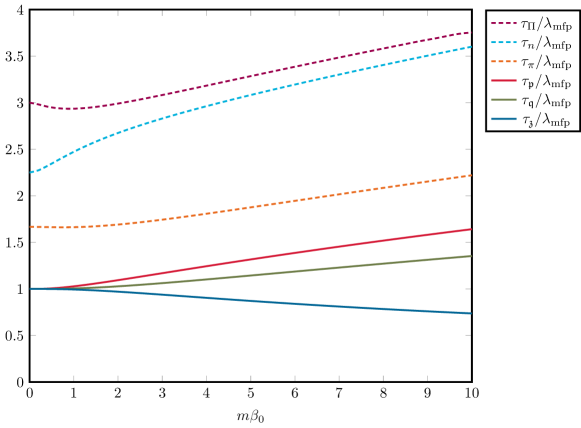
Figure 1: Relaxation times for the dissipative components of the spin tensor $\mathfrak{p}^{\mu}$, $\mathfrak{z}^{\mu\nu}$, $\mathfrak{q}^{\lambda\mu\nu}$ (full lines), in comparison to those for the standard dissipative quantities $\Pi$, $n^{\mu}$, $\pi^{\mu\nu}$ (dashed lines) in the 14+24-moment approximation. Note that the values for $\tau_{n}$ and $\tau_{\pi}$ in the limit $m\beta_{0}\to 0$ agree with those obtained in Ref. Denicol et al. (2012b).

X Pauli-Lubanski vector

Comparing the polarization of hadrons measured in heavy-ion collisions with theoretical calculations requires knowledge of the so-called Pauli-Lubanski vector Becattini et al. (2013b); Becattini (2021); Speranza and Weickgenannt (2021); Tinti and Florkowski (2020). The latter quantity can be expressed in terms of the axial-vector component of the Wigner function

$$\mathcal{A}^{\mu}(x,p)=\int dS(p)\,\mathfrak{s}^{\mu}f(x,p,\mathfrak{s})$$ (123)

as Becattini (2021); Speranza and Weickgenannt (2021); Tinti and Florkowski (2020)

$$\Pi^{\mu}(p)=\frac{1}{2\mathcal{N}}\int d\Sigma_{\lambda}p^{\lambda}\mathcal{A}^{\mu}(x,p)\;,$$ (124)

where $d\Sigma_{\lambda}$ denotes the integration over the freeze-out hypersurface and we defined

$$\mathcal{N}\equiv\int d\Sigma_{\lambda}p^{\lambda}\int dS(p)f(x,p,\mathfrak{s})\;.$$ (125)

Inserting the distribution function (66) and using the 14+24-moment approximation, we obtain

$$\Pi^{\mu}(p)= \frac{1}{2\mathcal{N}}\int d\Sigma_{\lambda}p^{\lambda}f_{0p}\bigg{[}-\frac{\hbar}{2m}\tilde{\Omega}^{\mu\rho}\left(E_{p}u_{\rho}+p_{\langle\rho\rangle}\right)+\left(g^{\mu}_{\nu}-\frac{p_{\langle\nu\rangle}}{E_{p}}u^{\mu}\right)\Big{(}\chi_{\mathfrak{p}}\mathfrak{p}^{\langle\nu\rangle}-6\chi_{\mathfrak{n}}\mathfrak{q}^{\rho\nu}_{\ \ \rho}+\chi_{\mathfrak{z}}\mathfrak{z}^{\nu\alpha}p_{\langle\alpha\rangle}$$

$$+\chi_{\mathfrak{q}}\mathfrak{q}^{\langle\nu\rangle\alpha\beta}p_{\langle\alpha}p_{\beta\rangle}\Big{)}\bigg{]}$$ (126)

where we defined

$$\chi_{\mathfrak{p}} \equiv-2\sum_{n\in\mathbb{S}_{0}}\mathcal{H}_{pn}^{(0)}\left(\mathfrak{F}_{n0}^{(0)}-\frac{1}{2}m^{2}\mathfrak{F}_{n2}^{(0)}\right)\;,$$

$$\chi_{\mathfrak{n}} \equiv-\frac{1}{2}\sum_{n\in\mathbb{S}_{0}}\mathcal{H}_{pn}^{(0)}\mathfrak{F}_{n2}^{(0)}\;,$$

$$\chi_{\mathfrak{z}} \equiv-\sum_{n\in\mathbb{S}_{1}}\mathcal{H}_{pn}^{(1)}\mathfrak{F}_{n1}^{(1)}\;,$$

$$\chi_{\mathfrak{q}} \equiv-2\sum_{n\in\mathbb{S}_{2}}\mathcal{H}_{pn}^{(2)}\mathfrak{F}_{n0}^{(2)}\;.$$ (127)

In the theory of second-order dissipative spin hydrodynamics, the spin moments are treated dynamically and follow the equations of motion derived in Sec. IX. On long time scales, they approach their Navier-Stokes values, namely the first-order terms on the right-hand sides of Eqs. (119), (120), and (121), respectively, cf. Sec. XI.

The global polarization is given as

$$\bar{\Pi}^{\mu}=\frac{1}{2{N}}\int d\Gamma\int d\Sigma_{\lambda}p^{\lambda}\,\mathfrak{s}^{\mu}f(x,p,\mathfrak{s})\;,$$ (128)

with $N\equiv\int dP\,\mathcal{N}$. We obtain

$$\bar{\Pi}^{\mu}= \frac{1}{2N}\int d\Sigma_{\lambda}\left[-u^{\lambda}\frac{\hbar}{2m}\omega_{0}^{\mu}I_{20}+\frac{\hbar}{2m}\Delta^{\lambda}_{\nu}\tilde{\Omega}^{\mu\nu}I_{21}+u^{\lambda}\left(\mathfrak{y}_{\mathfrak{p}}\mathfrak{p}^{\langle\mu\rangle}+\mathfrak{y}_{\mathfrak{q}}\mathfrak{q}^{\rho\mu}_{\ \ \rho}-\mathfrak{y}_{\mathfrak{z}}u^{\mu}\mathfrak{z}^{\rho}_{\ \rho}\right)+\mathfrak{y}_{\mathfrak{z}}\mathfrak{z}^{\mu\lambda}+u^{\mu}\left(\mathfrak{w}_{\mathfrak{p}}\mathfrak{p}^{\langle\lambda\rangle}+\mathfrak{w}_{\mathfrak{q}}\mathfrak{q}^{\rho\lambda}_{\ \ \rho}\right)\right]\;,$$ (129)

with

$$\mathfrak{y}_{\mathfrak{p}} \equiv\mathfrak{F}_{10}^{(0)}-\frac{1}{2}m^{2}\mathfrak{F}_{12}^{(0)}\;, \mathfrak{y}_{\mathfrak{q}} \equiv-\frac{3}{2}\mathfrak{F}_{12}^{(0)}\;, \mathfrak{y}_{\mathfrak{z}} \equiv\frac{1}{2}\mathfrak{F}_{01}^{(1)}\;,$$

$$\mathfrak{w}_{\mathfrak{p}} \equiv-\frac{1}{3}\left(m^{2}\mathfrak{F}_{-10}^{(0)}-\mathfrak{F}_{10}^{(0)}\right)+\frac{m^{2}}{6}\left(m^{2}\mathfrak{F}_{-12}^{(0)}-\mathfrak{F}_{12}^{(0)}\right)\;, \mathfrak{w}_{\mathfrak{q}} \equiv-\mathfrak{F}_{-10}^{(2)}+\frac{1}{2}\left(m^{2}\mathfrak{F}^{(0)}_{-12}-\mathfrak{F}^{(0)}_{12}\right)\;.$$ (130)

We remark that, although the form of the Pauli-Lubanski vector given by Eq. (124) is independent of the choice of pseudo-gauge, the truncation scheme used in a hydrodynamic framework can implicitly induce a pseudo-gauge dependence on the polarization, see also Refs. Becattini et al. (2019b); Becattini (2021); Speranza and Weickgenannt (2021); Buzzegoli (2022) for related discussions. In our case, the pseudo-gauge dependence enters through the choice of dynamical spin moments in the expansion of the distribution function in Eq. (126).

XI Navier-Stokes limit

The Navier-Stokes limit is obtained by considering only terms up to first order in gradients in the equations of motion in Sec. IX. In this context it is important to note that, in our power-counting scheme, the vorticity is considered to be different than standard gradients, cf. Sec. IV, which allows to account for a global-equilibrium state with arbitrary rotation. Thus, we neglect terms of linear order in the product of gradients and dissipative quantities, e.g., terms like $\nabla^{\lambda}\tau_{r}^{\nu,\mu_{1}\cdots\mu_{n}}$. However, this does not pertain to terms of linear order in the product of vorticity and dissipative quantities as, for instance, appear in expressions $\sim\nabla^{\lambda}\Delta^{\lambda}_{\alpha}\tau_{r}^{\alpha,\mu_{1}\cdots\mu_{n}}$, where the space-like gradient also acts on the three-space projector. Therefore we have in the Navier-Stokes limit

$$\mathfrak{p}^{{\langle\mu\rangle}}_{\text{NS}} =\mathfrak{p}^{\langle\mu\rangle}_{\text{nr}}\;,$$ (131a)

$$\mathfrak{z}^{\mu\nu}_{\text{NS}} =\mathfrak{z}^{\mu\nu}_{\text{nr}}+\tau_{\mathfrak{z}}\omega^{\ (\nu}_{\rho}\mathfrak{z}^{\mu)\rho}_{\text{NS}}\;,$$ (131b)

$$\mathfrak{q}^{{\langle\mu\rangle}\nu\lambda}_{\text{NS}} =\mathfrak{q}^{{\langle\mu\rangle}\nu\lambda}_{\text{nr}}-2\tau_{\mathfrak{q}}\mathfrak{q}_{\text{NS}}^{{\langle\mu\rangle}\rho\langle\nu}\omega^{\lambda\rangle}_{\ \rho}\;,$$ (131c)

with

$$\mathfrak{p}^{\langle\mu\rangle}_{\text{nr}} =\mathfrak{e}^{(0)}\left(\tilde{\Omega}^{\mu\nu}-\tilde{\varpi}^{\mu\nu}\right)u_{\nu}+\mathfrak{K}^{(0)}_{\theta\omega}\theta\omega_{0}^{\mu}+\mathfrak{K}^{(0)}_{I\Omega}I_{\nu}\tilde{\Omega}^{{\langle\mu\rangle}\nu}+\mathfrak{K}^{(0)}_{\nabla\Omega}\Delta^{\mu}_{\lambda}\nabla_{\nu}\tilde{\Omega}^{\lambda\nu}+\mathfrak{K}^{(0)}_{\dot{\Omega}}\dot{\omega}_{0}^{\langle\mu\rangle}\;,$$ (132a)

$$\mathfrak{z}^{\mu\nu}_{\text{nr}} =-\mathfrak{K}^{(1)}_{\nabla\Omega}\Delta^{(\mu}_{\rho}\left(\nabla^{\nu)}\tilde{\Omega}^{\rho\lambda}\right)u_{\lambda}-\mathfrak{K}^{(1)}_{\omega I}I^{(\nu}\omega_{0}^{\mu)}+\mathfrak{K}_{\Omega\sigma}^{(1)}\tilde{\Omega}^{\ (\langle\mu\rangle}_{\lambda}\sigma^{\nu)\lambda}\;,$$ (132b)

$$\mathfrak{q}^{{\langle\mu\rangle}\nu\lambda}_{\text{nr}} =-\mathfrak{d}^{(2)}\beta_{0}\sigma_{\rho}^{\ \langle\nu}\epsilon^{\lambda\rangle\mu\alpha\rho}u_{\alpha}+\mathfrak{K}_{\Omega I}^{(2)}\tilde{\Omega}^{{\langle\mu\rangle}\langle\nu}I^{\lambda\rangle}+\mathfrak{K}_{\nabla\Omega}^{(2)}\Delta^{\mu}_{\rho}\Delta^{\nu\lambda}_{\alpha\beta}\nabla^{\alpha}\tilde{\Omega}^{\rho\beta}-\mathfrak{K}_{\omega\sigma}^{(2)}\sigma^{\nu\lambda}\omega_{0}^{\mu}\;,$$ (132c)

being the Navier-Stokes values for relaxation to a nonrotating equilibrium state. The first terms on the right-hand sides of Eqs. (132a) and (132c) arise from the nonlocal collision term (107). This is also apparent from the fact that the coefficient $\mathfrak{e}^{(0)}$ is of order $\sim\Delta/\beta_{0}$ times the dimension of $\mathfrak{p}^{\mu}$, while $\mathfrak{d}^{(2)}$ is of order $\sim\Delta/\beta_{0}$ times the dimension of $\mathfrak{q}^{\mu\nu\lambda}$. This follows from the definition of these quantities in Eqs. (152b) and (154b) and the fact that $\tau_{\mathfrak{p}}$ and $\tau_{\mathfrak{q}}$ are of order $\sim\lambda_{\text{mfp}}$, while $g^{(0)}_{0}$ and $h_{0}^{(2)}$, cf. Eqs. (109a) and (109d), are $\sim\Delta/\lambda_{\text{mfp}}$ times appropriate powers of temperature to give the correct dimensions. Thus, the first terms on the right-hand sides of Eqs. (132a) and (132c) are of order $\sim\Delta/L_{\text{hydro}}$ times the dimensions of $\mathfrak{p}^{\mu}$ and $\mathfrak{q}^{\mu\nu\lambda}$, respectively. On the other hand, the other terms $\sim\mathfrak{K}^{(l)}_{i}$ in Eqs. (132a) – (132c) are of order $\sim(\Delta/L_{\text{hydro}})(\lambda_{\text{mfp}}/\ell_{\text{vort}})$ times the dimensions of $\mathfrak{p}^{\mu}$ and $\mathfrak{q}^{\mu\nu\lambda}$, respectively. While this is formally of order $\text{Kn}^{2}$, cf. Eq. (36), we cannot simply neglect this term, as one would usually do for the Navier-Stokes limit. The reason is that in our power-counting scheme we were not forced to specify the ratio $\lambda_{\text{mfp}}/\ell_{\text{vort}}$, such that in principle it can be of order unity. Then, the terms $\sim\mathfrak{K}^{(l)}_{i}$ are of the same order as the first terms $\sim\mathfrak{e}^{(0)},\,\mathfrak{d}^{(2)}$. Only if $\lambda_{\text{mfp}}/\ell_{\text{vort}}\ll 1$, we may drop these terms.

We note that, when inserting Eq. (132c) into Eq. (126), we obtain a term

$$\Pi^{\mu}(p)\ni\int d\Sigma_{\lambda}p^{\lambda}f_{0p}\chi_{\mathfrak{q}}\mathfrak{d}^{(2)}\beta_{0}\epsilon^{\mu\beta\sigma\rho}u_{\sigma}\sigma_{\rho}^{\ \alpha}p_{\langle\alpha}p_{\beta\rangle}\;.$$ (133)

This term has a similar structure as the coupling term between spin and thermal shear obtained in Refs. Liu and Yin (2021); Fu et al. (2021); Becattini et al. (2021a, b). As we have just argued, this term arises from the nonlocal collision term and thus is of order $\sim\Delta/L_{\text{hydro}}$ ($\chi_{\mathfrak{q}}$ is just a combination of thermodynamic integrals). However, due to the fact that it arises from collisions we are hesitant to call such a term nondissipative. Therefore, it may have a different origin in the approach of Refs. Liu and Yin (2021); Fu et al. (2021); Becattini et al. (2021a, b). We remark that the contribution (133) to the local polarization vanishes after integration over four-momentum, therefore it does not affect the global polarization (128).

The solution of Eqs. (131) is obtained analogously to the calculation outlined in Ref. Denicol et al. (2018) as

$$\mathfrak{z}^{\mu\nu}_{\text{NS}}= \left[2\lambda_{0}\Delta^{\mu\nu\alpha\beta}+\lambda_{1}\left(\Delta^{\mu\nu}-\frac{3}{2}\Xi^{\mu\nu}\right)\left(\Delta^{\alpha\beta}-\frac{3}{2}\Xi^{\alpha\beta}\right)-2\lambda_{2}\Xi^{\alpha(\mu}\hat{\omega}^{\nu)}\hat{\omega}^{\beta}-2\lambda_{3}\Xi^{\alpha(\mu}\hat{\omega}^{\nu)\beta}+2\lambda_{4}\hat{\omega}^{\alpha(\mu}\hat{\omega}^{\nu)}\hat{\omega}^{\beta}\right.$$

$$\left.+\frac{1}{3}\Delta^{\mu\nu}\Delta^{\alpha\beta}\right]\mathfrak{z}_{\text{nr}\alpha\beta}\;,$$ (134a)

$$\mathfrak{q}^{{\langle\mu\rangle}\nu\lambda}_{\text{NS}}= \left[2\eta_{0}\Delta^{\nu\lambda\alpha\beta}+\eta_{1}\left(\Delta^{\nu\lambda}-\frac{3}{2}\Xi^{\nu\lambda}\right)\left(\Delta^{\alpha\beta}-\frac{3}{2}\Xi^{\alpha\beta}\right)-2\eta_{2}\Xi^{\alpha(\nu}\hat{\omega}^{\lambda)}\hat{\omega}^{\beta}-2\eta_{3}\Xi^{\alpha(\nu}\hat{\omega}^{\lambda)\beta}+2\eta_{4}\hat{\omega}^{\alpha(\nu}\hat{\omega}^{\lambda)}\hat{\omega}^{\beta}\right]$$

$$\times\mathfrak{q}^{{\langle\mu\rangle}}_{\text{nr}\ \alpha\beta}\;,$$ (134b)

where we defined $\omega\equiv\sqrt{\omega^{\mu\nu}\omega_{\mu\nu}/2}$ and $\hat{\omega}^{\mu\nu}\equiv-\omega^{\mu\nu}/\omega$. Furthermore, we defined the unit vector along the vorticity direction $\hat{\omega}^{\mu}\equiv\omega^{\mu}/\omega$ and the projector orthogonal to both the fluid velocity and vorticity vector,

$$\Xi^{\mu\nu}\equiv g^{\mu\nu}-u^{\mu}u^{\nu}+\hat{\omega}^{\mu}\hat{\omega}^{\nu}\;.$$ (135)

The coefficients in Eqs. (134) are given in Appendix C.

XII Conclusions

In this paper, we derived the second-order dissipative equations of motion for relativistic spin hydrodynamics using the method of moments. The starting point was the quantum kinetic theory for massive spin-1/2 particles developed in Refs. Weickgenannt et al. (2019); Weickgenannt et al. (2021a, b), which takes into account nonlocal collisions. We constructed relativistic spin hydrodynamics using the HW pseudo-gauge for the energy-momentum and spin tensors. In our framework, we treated the components of the HW spin tensor as the dynamical variables of the theory. Furthermore, we argued that the choice of the pseudo-gauge affects the evolution of the system, since in different pseudo-gauges different moments are treated dynamically. The equations of motion of the HW spin tensor correspond to conservation laws in global equilibrium, unlike in the case of the canonical pseudo-gauge Speranza and Weickgenannt (2021). As a consequence, (at least some) spin dynamics must occur on large, i.e., hydrodynamic scales.

In order to define our expansion, we proposed a novel power-counting scheme, which generalizes the concept of local equilibrium in the presence of spin dynamics with nonlocal collisions. We then extended the method of moments presented in Ref. Denicol et al. (2012b) to include spin dynamics. In particular, we expanded the distribution function around a local-equilibrium state in terms of the usual irreducible moments in momentum space Denicol et al. (2012b) and, in addition, of so-called spin moments containing the phase-space variable $\mathfrak{s}^{\mu}$. For the truncation we chose the “14+24-moment approximation”, where “14” corresponds to the usual components of the charge current and the energy-momentum tensor and “24” to the components of the spin tensor. Our result is a closed set of equations of motion for the dynamical spin moments, where the latter approach their Navier-Stokes limits on time scales corresponding to characteristic relaxation times. Remarkably, the spin relaxation times are determined by the local part of the collision term in the Boltzmann equation. On the other hand, the nonlocal part, which is responsible for the mutual conversion of orbital angular momentum and spin, gives rise to terms which appear in the same way as the conventional Navier-Stokes terms, albeit their power counting is different: they are of order $\Delta/L_{\text{hydro}}$, not of order Kn. Moreover, we find that the spin relaxation times are comparable in magnitude to the relaxation times of the conventional dissipative quantities such as bulk, shear stress, and particle diffusion. This implies that it is reasonable to treat spin as dynamical variable in relativistic second-order spin hydrodynamics. Finally, we gave an expression for the Pauli-Lubanski vector which takes into account dissipative spin effects. In the Navier-Stokes limit, we obtained a coupling term between spin and the shear-stress tensor, similar as in Refs. Liu and Yin (2021); Fu et al. (2021); Becattini et al. (2021a, b), although the origin of this term in our approach may be different.

Our work establishes a theory of relativistic second-order dissipative spin hydrodynamics for applications in heavy-ion collisions as well as astrophysics. In particular, it can be used to solve and understand the puzzle related to the longitudinal polarization of Lambda particles. The equations of motion derived in this work provide the starting point for a numerical implementation of relativistic spin hydrodynamics. In this respect, a crucial future task is to analyze the conditions under which our theory of spin hydrodynamics is causal and stable. This is challenging because of the larger number of variables and equations of motion of relativistic spin hydrodynamics compared to the conventional case, and due to the presence of vorticity fields Speranza et al. (2021). It will also be interesting to investigate how the choice of different hydrodynamic frames (i.e., different matching conditions) Bemfica et al. (2018, 2019, 2020); Kovtun (2019); Hoult and Kovtun (2020); Speranza et al. (2021); Noronha et al. (2021) affect the theory presented here as far as its causality and stability is concerned. For a study regarding conventional relativistic hydrodynamics using the method of moments with general matching conditions see Ref. Rocha and Denicol (2021).

Appendix A Properties of irreducible tensors

In the calculations in Sec. VII we make use of the following relations Coope and Snider (1970):

$$p^{\mu} =E_{p}u^{\mu}+p^{\langle\mu\rangle}\;,$$ (136)

$$\Delta^{\alpha\beta}p_{\alpha}p_{\beta} =m^{2}-E_{p}^{2}\;,$$ (137)

$$p^{\langle\mu\rangle}p^{\langle\nu\rangle} =p^{\langle\mu}p^{\nu\rangle}+\frac{1}{3}(m^{2}-E_{p}^{2})\Delta^{\mu\nu}\;,$$ (138)

$$p^{\langle\mu\rangle}p^{\langle\nu\rangle}p^{\langle\lambda\rangle} =p^{\langle\mu}p^{\nu}p^{\lambda\rangle}+\frac{1}{5}(m^{2}-E_{p}^{2})\left(p^{\langle\mu\rangle}\Delta^{\nu\lambda}+p^{\langle\nu\rangle}\Delta^{\lambda\mu}+p^{\langle\lambda\rangle}\Delta^{\mu\nu}\right)\;,$$ (139)

$$p^{\langle\mu\rangle}p^{\langle\nu\rangle}p^{\langle\lambda\rangle}p^{\langle\rho\rangle} =p^{\langle\mu}p^{\nu}p^{\lambda}p^{\rho\rangle}+\frac{1}{7}\left(p^{\langle\mu\rangle}p^{\langle\nu\rangle}\Delta^{\lambda\rho}+p^{\langle\mu\rangle}p^{\langle\lambda\rangle}\Delta^{\nu\rho}+p^{\langle\mu\rangle}p^{\langle\rho\rangle}\Delta^{\lambda\nu}+p^{\langle\lambda\rangle}p^{\langle\nu\rangle}\Delta^{\mu\rho}+p^{\langle\rho\rangle}p^{\langle\nu\rangle}\Delta^{\lambda\mu}\right.$$

$$\left.+p^{\langle\lambda\rangle}p^{\langle\rho\rangle}\Delta^{\mu\nu}\right)(m^{2}-E_{p}^{2})-\frac{1}{35}\left(\Delta^{\mu\nu}\Delta^{\lambda\rho}+\Delta^{\mu\lambda}\Delta^{\nu\rho}+\Delta^{\mu\rho}\Delta^{\nu\lambda}\right)(m^{2}-E_{p}^{2})^{2}$$

$$=p^{\langle\mu}p^{\nu}p^{\lambda}p^{\rho\rangle}+\frac{1}{7}\left(p^{\langle\mu}p^{\nu\rangle}\Delta^{\lambda\rho}+p^{\langle\mu}p^{\lambda\rangle}\Delta^{\nu\rho}+p^{\langle\mu}p^{\rho\rangle}\Delta^{\lambda\nu}+p^{\langle\lambda}p^{\nu\rangle}\Delta^{\mu\rho}+p^{\langle\rho}p^{\nu\rangle}\Delta^{\lambda\mu}\right.$$

$$\left.+p^{\langle\lambda}p^{\rho\rangle}\Delta^{\mu\nu}\right)(m^{2}-E_{p}^{2})+\frac{1}{15}\left(\Delta^{\mu\nu}\Delta^{\lambda\rho}+\Delta^{\mu\lambda}\Delta^{\nu\rho}+\Delta^{\mu\rho}\Delta^{\nu\lambda}\right)(m^{2}-E_{p}^{2})^{2}\;,$$ (140)

$$p^{\langle\mu\rangle}p^{\langle\nu\rangle}p^{\langle\lambda\rangle}p^{\langle\rho\rangle}p^{\langle\sigma\rangle} =p^{\langle\mu}p^{\nu}p^{\lambda}p^{\rho}p^{\sigma\rangle}+\frac{1}{9}(m^{2}-E_{p}^{2})\left(p^{\langle\mu\rangle}p^{\langle\nu\rangle}p^{\langle\lambda\rangle}\Delta^{\rho\sigma}+\text{perm.}\right)$$

$$-\frac{1}{63}(m^{2}-E_{p}^{2})^{2}\left(p^{\langle\mu\rangle}\Delta^{\nu\lambda}\Delta^{\rho\sigma}+\text{perm}\right)$$

$$=p^{\langle\mu}p^{\nu}p^{\lambda}p^{\rho}p^{\sigma\rangle}+\frac{1}{9}(m^{2}-E_{p}^{2})\left(p^{\langle\mu}p^{\nu}p^{\lambda\rangle}\Delta^{\rho\sigma}+\text{perm.}\right)$$

$$+\frac{1}{35}(m^{2}-E_{p}^{2})^{2}\left(p^{\langle\mu\rangle}\Delta^{\nu\lambda}\Delta^{\rho\sigma}+\text{perm.}\right)\;,$$ (141)

where ”perm.” denotes all distinct permutations of indices. We also utilize the orthogonality relation

$$\int dP\,p^{\langle\mu_{1}}\cdots p^{\mu_{m}\rangle}p_{\langle\nu_{1}}\cdots p_{\nu_{n}\rangle}F(E_{p})=\frac{m!\delta_{mn}}{(2m+1)!!}\Delta^{\mu_{1}\cdots\mu_{m}}_{\nu_{1}\cdots\nu_{m}}\int dP\,\left(\Delta^{\alpha\beta}p_{\alpha}p_{\beta}\right)^{m}F(E_{p})$$ (143)

for an arbitrary function $F(E_{p})$.

Appendix B Scattering matrix elements

In this appendix we show some details of the calculation of the scattering matrix elements in the collision term. The vacuum scattering matrix elements are defined as Siskens and Van Weert (1977); De Groot et al. (1980)

$$\langle{p,p^{\prime};r,r^{\prime}|t|p_{1},p_{2};s_{1},s_{2}}\rangle=\langle{p,p^{\prime};r,r^{\prime}|:{H}_{I}(0):|p_{1},p_{2};s_{1},s_{2}}\rangle\;,$$ (144)

where $H_{I}$ is the effective interaction Hamiltonian, which is here taken to be of an NJL-type form Nambu and Jona-Lasinio (1961a, b)

$$H_{I}(x)=G\,\bar{\psi}(x)\Gamma^{a}\psi(x)\,\bar{\psi}(x)\Gamma_{a}\psi(x)\;,$$ (145)

where $G$ is a coupling constant and $\Gamma_{a}$ is in general a linear combination of elements of the Clifford algebra in a given representation of the Lorentz group, e.g., for scalar interactions $\Gamma^{a}=1$, for vector interactions $\Gamma^{a}=\gamma^{\mu}$, and for parity-violating interactions $\Gamma^{a}=(1-\gamma_{5})\gamma^{\mu}$. Inserting the free-field expansion of the spinors,

$$\psi(x)=\sqrt{\frac{2}{(2\pi\hbar)^{3}}}\sum_{r}\int dP\,e^{-\frac{i}{\hbar}p\cdot x}u_{r}(p)a_{r}(p)\;,$$ (146)

and making use of the anticommutation relation of the creation and annihilation operators

$$\{a_{r}(p),a^{\dagger}_{s}(p^{\prime})\}=p^{0}\delta^{(3)}(\mathbf{p}-\mathbf{p}^{\prime})\delta_{rs}\;,$$ (147)

we find

$$\langle{p,p^{\prime};r,r^{\prime}|t|p_{1},p_{2};r_{1},r_{2}}\rangle= \bar{G}\left[\bar{u}_{r}(p)\Gamma^{a}u_{r_{2}}(p_{2})\bar{u}_{r^{\prime}}(p^{\prime})\Gamma_{a}u_{r_{1}}(p_{1})-\bar{u}_{r}(p)\Gamma^{a}u_{r_{1}}(p_{1})\bar{u}_{r^{\prime}}(p^{\prime})\Gamma_{a}u_{r_{2}}(p_{2})\right]\;,$$ (148)

with $\bar{G}\equiv 8/(2\pi\hbar)^{6}G$. For Eq. (101a) we then obtain using Eq. (5)

$$\int[dS]\,\mathcal{W}= |\bar{G}|^{2}\delta^{(4)}(p+p^{\prime}-p_{1}-p_{2})\,\left[\bar{u}_{r}(p)\Gamma^{a}u_{r_{2}}(p_{2})\bar{u}_{r^{\prime}}(p^{\prime})\Gamma_{a}u_{r_{1}}(p_{1})-\bar{u}_{r}(p)\Gamma^{a}u_{r_{1}}(p_{1})\bar{u}_{r^{\prime}}(p^{\prime})\Gamma_{a}u_{r_{2}}(p_{2})\right]$$

$$\times\left[\bar{u}_{r}(p)\Gamma^{b}u_{r_{2}}(p_{2})\bar{u}_{r^{\prime}}(p^{\prime})\Gamma_{b}u_{r_{1}}(p_{1})-\bar{u}_{r}(p)\Gamma^{b}u_{r_{1}}(p_{1})\bar{u}_{r^{\prime}}(p^{\prime})\Gamma_{b}u_{r_{2}}(p_{2})\right]^{\dagger}$$

$$= |\bar{G}|^{2}\delta^{(4)}(p+p^{\prime}-p_{1}-p_{2})\,\bigg{\{}\text{Tr}\left[\left(\not{p}+m\right)\Gamma^{a}\left(\not{p}_{2}+m\right)\Gamma^{b}\right]\text{Tr}\left[\left(\not{p}^{\prime}+m\right)\Gamma_{a}\left(\not{p}_{1}+m\right)\Gamma_{b}\right]$$

$$-\text{Tr}\left[\left(\not{p}+m\right)\Gamma^{a}\left(\not{p}_{2}+m\right)\Gamma_{b}\left(\not{p}^{\prime}+m\right)\Gamma_{a}\left(\not{p}_{1}+m\right)\Gamma^{b}\right]$$

$$-\text{Tr}\left[\left(\not{p}+m\right)\Gamma^{a}\left(\not{p}_{1}+m\right)\Gamma_{b}\left(\not{p}^{\prime}+m\right)\Gamma_{a}\left(\not{p}_{2}+m\right)\Gamma^{b}\right]$$

$$+\text{Tr}\left[\left(\not{p}+m\right)\Gamma^{a}\left(\not{p}_{1}+m\right)\Gamma^{b}\right]\text{Tr}\left[\left(\not{p}^{\prime}+m\right)\Gamma_{a}\left(\not{p}_{2}+m\right)\Gamma_{b}\right]\bigg{\}}\;.$$ (149)

Furthermore we have for Eq. (101b)

$$\int[dS]\,\mathfrak{s}^{\alpha}\mathcal{W}= -|\bar{G}|^{2}\delta^{(4)}(p+p^{\prime}-p_{1}-p_{2})\,\left[\bar{u}_{r}(p)\Gamma^{a}u_{r_{2}}(p_{2})\bar{u}_{r^{\prime}}(p^{\prime})\Gamma_{a}u_{r_{1}}(p_{1})-\bar{u}_{r}(p)\Gamma^{a}u_{r_{1}}(p_{1})\bar{u}_{r^{\prime}}(p^{\prime})\Gamma_{a}u_{r_{2}}(p_{2})\right]$$

$$\times\left[\bar{u}_{s}(p)\Gamma^{b}u_{r_{2}}(p_{2})\bar{u}_{r^{\prime}}(p^{\prime})\Gamma_{b}u_{r_{1}}(p_{1})-\bar{u}_{s}(p)\Gamma^{b}u_{r_{1}}(p_{1})\bar{u}_{r^{\prime}}(p^{\prime})\Gamma_{b}u_{r_{2}}(p_{2})\right]^{\dagger}\frac{1}{2m}\bar{u}_{s}(p)\gamma^{5}\gamma^{\alpha}u_{r}(p)$$

$$= -\frac{|\bar{G}|^{2}}{2m}\delta^{(4)}(p+p^{\prime}-p_{1}-p_{2})\,\bigg{\{}\text{Tr}\left[\left(\not{p}+m\right)\gamma^{5}\gamma^{\alpha}\left(\not{p}+m\right)\Gamma^{a}\left(\not{p}_{2}+m\right)\Gamma^{b}\right]$$

$$\times\text{Tr}\left[\left(\not{p}^{\prime}+m\right)\Gamma_{a}\left(\not{p}_{1}+m\right)\Gamma_{b}\right]$$

$$-\text{Tr}\left[\left(\not{p}+m\right)\gamma^{5}\gamma^{\alpha}\left(\not{p}+m\right)\Gamma^{a}\left(\not{p}_{2}+m\right)\Gamma_{b}\left(\not{p}^{\prime}+m\right)\Gamma_{a}\left(\not{p}_{1}+m\right)\Gamma^{b}\right]$$

$$-\text{Tr}\left[\left(\not{p}+m\right)\gamma^{5}\gamma^{\alpha}\left(\not{p}+m\right)\Gamma^{a}\left(\not{p}_{1}+m\right)\Gamma_{b}\left(\not{p}^{\prime}+m\right)\Gamma_{a}\left(\not{p}_{2}+m\right)\Gamma^{b}\right]$$

$$+\text{Tr}\left[\left(\not{p}+m\right)\gamma^{5}\gamma^{\alpha}\left(\not{p}+m\right)\Gamma^{a}\left(\not{p}_{1}+m\right)\Gamma^{b}\right]\text{Tr}\left[\left(\not{p}^{\prime}+m\right)\Gamma_{a}\left(\not{p}_{2}+m\right)\Gamma_{b}\right]\bigg{\}}\;,$$ (150)

and for Eq. (101c)

$$\int[dS]\,\mathfrak{s}^{\alpha}\mathfrak{s}^{\prime\beta}\mathcal{W}= \frac{|\bar{G}|^{2}}{(2m)^{2}}\delta^{(4)}(p+p^{\prime}-p_{1}-p_{2})\,\bigg{\{}\text{Tr}\left[\left(\not{p}+m\right)\gamma^{5}\gamma^{\alpha}\left(\not{p}+m\right)\Gamma^{a}\left(\not{p}_{2}+m\right)\Gamma^{b}\right]$$

$$\times\text{Tr}\left[\left(\not{p}^{\prime}+m\right)\gamma^{5}\gamma^{\beta}\left(\not{p}^{\prime}+m\right)\Gamma_{a}\left(\not{p}_{1}+m\right)\Gamma_{b}\right]$$

$$-\text{Tr}\left[\left(\not{p}+m\right)\gamma^{5}\gamma^{\alpha}\left(\not{p}+m\right)\Gamma^{a}\left(\not{p}_{2}+m\right)\Gamma_{b}\left(\not{p}^{\prime}+m\right)\gamma^{5}\gamma^{\beta}\left(\not{p}^{\prime}+m\right)\Gamma_{a}\left(\not{p}_{1}+m\right)\Gamma^{b}\right]$$

$$-\text{Tr}\left[\left(\not{p}+m\right)\gamma^{5}\gamma^{\alpha}\left(\not{p}+m\right)\Gamma^{a}\left(\not{p}_{1}+m\right)\Gamma_{b}\left(\not{p}^{\prime}+m\right)\gamma^{5}\gamma^{\beta}\left(\not{p}^{\prime}+m\right)\Gamma_{a}\left(\not{p}_{2}+m\right)\Gamma^{b}\right]$$

$$+\text{Tr}\left[\left(\not{p}+m\right)\gamma^{5}\gamma^{\alpha}\left(\not{p}+m\right)\Gamma^{a}\left(\not{p}_{1}+m\right)\Gamma^{b}\right]\text{Tr}\left[\left(\not{p}^{\prime}+m\right)\gamma^{5}\gamma^{\beta}\left(\not{p}^{\prime}+m\right)\Gamma_{a}\left(\not{p}_{2}+m\right)\Gamma_{b}\right]\bigg{\}}\;.$$ (151)

In the case of a scalar intercation, $\Gamma^{a}=1$, evaluating the traces of Dirac matrices yields that Eqs. (150) and (151) vanish, respectively. For a vector interaction, $\Gamma^{a}=\gamma^{\mu}$, Eq. (150) also vanishes, while Eq. (151) is nonzero. However, in the limit of small momentum transfer ($s=4m^{2}$, $t=u=0$) Eq. (151) is zero also for the vector interaction, while the only nonzero contribution comes from Eq. (149).

Appendix C Transport coefficients

The relaxation times and transport coefficients in Eq. (119) are given by

$$\tau_{\mathfrak{p}} =\mathfrak{T}_{00}^{(0)}\;,$$ (152a)

$$\mathfrak{e}^{(0)} =\tau_{\mathfrak{p}}\,g_{0}^{(0)}\;,$$ (152b)

$$\mathfrak{K}^{(0)}_{\theta\omega} =\frac{\hbar}{2m}\tau_{\mathfrak{p}}\,\xi_{0}^{(0)}\;,$$ (152c)

$$\mathfrak{K}^{(0)}_{\theta\omega\Pi} =\frac{\hbar}{2m}\,\frac{G_{21}}{D_{20}}\tau_{\mathfrak{p}}=-\mathfrak{K}^{(0)}_{\pi\sigma\omega}\;,$$ (152d)

$$\mathfrak{K}^{(0)}_{n\omega} =-\frac{\hbar}{2m}\,\frac{G_{30}}{D_{20}}\tau_{\mathfrak{p}}\;,$$ (152e)

$$\mathfrak{K}^{(0)}_{I\Omega} =-\frac{\hbar}{4m}I_{11}\tau_{\mathfrak{p}}=\mathfrak{K}^{(0)}_{\nabla\Omega}\;,$$ (152f)

$$\mathfrak{K}^{(0)}_{\Pi\Omega} =\frac{\hbar}{4m}\frac{\beta_{0}I_{21}}{\epsilon_{0}+P_{0}}\tau_{\mathfrak{p}}\;,$$ (152g)

$$\mathfrak{K}^{(0)}_{\dot{\Omega}} =-\frac{\hbar}{4m}I_{10}\tau_{\mathfrak{p}}\;,$$ (152h)

$$\mathfrak{g}^{(0)}_{1} =\frac{1}{2}\tau_{\mathfrak{p}}\frac{\partial\mathfrak{F}_{-11}^{(1)}}{\partial\beta_{0}}\frac{\beta_{0}}{\epsilon_{0}+P_{0}}\;,$$ (152i)

$$\mathfrak{g}^{(0)}_{2} =-\tau_{\mathfrak{p}}\mathfrak{F}_{-20}^{(2)}\;,$$ (152j)

$$\mathfrak{g}^{(0)}_{3} =\frac{1}{2}\tau_{\mathfrak{p}}\mathfrak{F}_{-11}^{(1)}\;,$$ (152k)

$$\mathfrak{g}^{(0)}_{4} =-\frac{1}{9}\tau_{\mathfrak{p}}\left(7-4m^{2}\mathfrak{F}_{-20}^{(0)}+2m^{4}\mathfrak{F}_{-22}^{(0)}\right)\;,$$ (152l)

$$\mathfrak{g}^{(0)}_{5} =\frac{1}{3}\tau_{\mathfrak{p}}\left(2m^{2}\mathfrak{F}_{-22}^{(0)}-\mathfrak{F}_{-20}^{(2)}\right)\;,$$ (152m)

$$\mathfrak{g}^{(0)}_{6} =-\frac{1}{2}\tau_{\mathfrak{p}}\left(\frac{\partial\mathfrak{F}_{-11}^{(1)}}{\partial\alpha_{0}}+\frac{\partial\mathfrak{F}_{-11}^{(1)}}{\partial\beta_{0}}\frac{n_{0}}{\epsilon_{0}+P_{0}}\right)\;,$$ (152n)

$$\mathfrak{g}_{7}^{(0)} =\frac{1}{3}\tau_{\mathfrak{p}}\left(m^{2}\mathfrak{F}_{-20}^{(0)}-1-\frac{1}{2}m^{4}\mathfrak{F}_{-22}^{(0)}\right)\;,$$ (152o)

$$\mathfrak{g}_{8}^{(0)} =\tau_{\mathfrak{p}}\left(\mathfrak{F}_{-20}^{(2)}-\frac{1}{2}m^{2}\mathfrak{F}^{(0)}_{-22}\right)\;,$$ (152p)

$$\mathfrak{g}_{9}^{(0)} =\frac{1}{2(\epsilon_{0}+P_{0})}\tau_{\mathfrak{p}}\mathfrak{F}^{(1)}_{-11}\;.$$ (152q)

Furthermore, the relaxation time and transport coefficients of Eq. (120) read

$$\tau_{\mathfrak{z}} =\mathfrak{T}_{11}^{(1)}\;,$$ (153a)

$$\mathfrak{K}_{\omega\Pi}^{(1)} ={\frac{\hbar}{2m}}\frac{\beta_{0}I_{41}}{\epsilon_{0}+P_{0}}\tau_{\mathfrak{z}}\;,$$ (153b)

$$\mathfrak{K}_{\omega I}^{(1)} ={\frac{\hbar}{2m}}\frac{\beta_{0}I_{31}}{\epsilon_{0}+P_{0}}\tau_{\mathfrak{z}}\;,$$ (153c)

$$\mathfrak{K}_{\Omega\sigma}^{(1)} =-{\frac{\hbar}{2m}}\beta_{0}I_{42}\tau_{\mathfrak{z}}\;,$$ (153d)

$$\mathfrak{K}_{\nabla\Omega}^{(1)} ={\frac{\hbar}{4m}}I_{31}\tau_{\mathfrak{z}}\;,$$ (153e)

$$\mathfrak{g}_{1}^{(1)} =-\frac{4}{3}\tau_{\mathfrak{z}}\;,$$ (153f)

$$\mathfrak{g}_{2}^{(1)} =-\tau_{\mathfrak{z}}\;,$$ (153g)

$$\mathfrak{g}_{3}^{(1)} =\frac{1}{5}\tau_{\mathfrak{z}}\,\left(m^{2}\mathfrak{F}_{-11}^{(1)}-1\right)\;,$$ (153h)

$$\mathfrak{g}_{4}^{(1)} =\tau_{\mathfrak{z}}\,\frac{1}{\epsilon_{0}+P_{0}}\;,$$ (153i)

$$\mathfrak{g}_{5}^{(1)} =-\frac{1}{2}\tau_{\mathfrak{z}}\,\;,$$ (153j)

$$\mathfrak{g}_{6}^{(1)} =\frac{3}{2}\frac{m^{2}}{(\epsilon_{0}+P_{0})}\tau_{\mathfrak{z}}\;,$$ (153k)

$$\mathfrak{g}_{7}^{(1)} =\frac{7}{2}\frac{1}{\epsilon_{0}+P_{0}}\tau_{\mathfrak{z}}\;,$$ (153l)

$$\mathfrak{g}_{8}^{(1)} =-\frac{1}{2}m^{2}\tau_{\mathfrak{z}}\;,$$ (153m)

$$\mathfrak{g}_{9}^{(1)} =-\frac{1}{2}\tau_{\mathfrak{z}}\;,$$ (153n)

$$\mathfrak{g}_{10}^{(1)} =\frac{1}{6}\tau_{\mathfrak{z}}\left(m^{2}\mathfrak{F}_{-11}^{(1)}-1\right)\;.$$ (153o)

Finally, the relaxation time and transport coefficients in Eq. (121) are

$$\tau_{\mathfrak{q}} =\mathfrak{T}_{00}^{(2)}\;,$$ (154a)

$$\mathfrak{d}^{(2)} =\tau_{\mathfrak{q}}\,h_{0}^{(2)}\;,$$ (154b)

$$\mathfrak{K}_{\Omega I}^{(2)} =\frac{\hbar}{2m}\tau_{\mathfrak{q}}\,\xi_{0}^{(2)}\;,$$ (154c)

$$\mathfrak{K}_{\nabla\Omega}^{(2)} ={\frac{\hbar}{2m}}I_{32}\tau_{\mathfrak{q}}\;,$$ (154d)

$$\mathfrak{K}_{\omega\sigma}^{(2)} =\frac{\hbar}{2m}\beta_{0}I_{42}\tau_{\mathfrak{q}}\;,$$ (154e)

$$\mathfrak{K}_{\Omega\Pi}^{(2)} =\frac{\hbar}{2m}\frac{\beta_{0}I_{42}}{\epsilon_{0}+P_{0}}\tau_{\mathfrak{q}}\;,$$ (154f)

$$\mathfrak{g}_{1}^{(2)} =\frac{1}{5}\tau_{\mathfrak{q}}\frac{1}{\epsilon_{0}+P_{0}}\left(m^{2}\mathfrak{F}^{(1)}_{-11}-5\mathfrak{F}^{(1)}_{11}+m^{2}\frac{\partial\mathfrak{F}^{(1)}_{-11}}{\partial\beta_{0}}\beta_{0}\right)\;,$$ (154g)

$$\mathfrak{g}_{2}^{(2)} =-\frac{m^{2}}{5}\tau_{\mathfrak{q}}\left(\frac{\partial\mathfrak{F}^{(1)}_{-11}}{\partial\alpha_{0}}+\frac{n_{0}}{\epsilon_{0}+P_{0}}\frac{\partial\mathfrak{F}^{(1)}_{-11}}{\partial\beta_{0}}\right)\;,$$ (154h)

$$\mathfrak{g}_{3}^{(2)} =\frac{1}{5}\tau_{\mathfrak{q}}\left(\mathfrak{F}^{(1)}_{11}-m^{2}\mathfrak{F}^{(1)}_{-11}\right)\;,$$ (154i)

$$\mathfrak{g}_{4}^{(2)} =\frac{1}{3}\tau_{\mathfrak{q}}\left(-m^{2}\mathfrak{F}^{(2)}_{-20}-4\right)\;,$$ (154j)

$$\mathfrak{g}_{5}^{(2)} =\frac{2}{7}\tau_{\mathfrak{q}}\left(-2m^{2}\mathfrak{F}^{(2)}_{-20}-5\right)\;,$$ (154k)

$$\mathfrak{g}_{6}^{(2)} =\frac{2m^{2}}{15}\tau_{\mathfrak{q}}\left(\frac{1}{2}m^{4}\mathfrak{F}^{(0)}_{-22}-m^{2}\mathfrak{F}^{(0)}_{-20}-5\right)\;,$$ (154l)

$$\mathfrak{g}_{7}^{(2)} =\frac{2}{15}\tau_{\mathfrak{q}}\left(1-\frac{m^{4}}{4}\mathfrak{F}^{(0)}_{-22}\right)\;,$$ (154m)

$$\mathfrak{g}_{8}^{(2)} =\frac{1}{5(\epsilon_{0}+P_{0})}\tau_{\mathfrak{q}}\left(m^{2}\mathfrak{F}^{(1)}_{-11}-1\right)\;,$$ (154n)

$$\mathfrak{g}_{9}^{(2)} =-\frac{2}{15}\tau_{\mathfrak{q}}\left(\frac{5}{2}m^{2}-m^{4}\mathfrak{F}^{(2)}_{-20}+\frac{1}{2}m^{6}\mathfrak{F}^{(0)}_{-22}\right)\;,$$ (154o)

$$\mathfrak{g}_{10}^{(2)} =\frac{2}{5}\tau_{\mathfrak{q}}\left(-\frac{3}{2}+m^{2}\mathfrak{F}^{(2)}_{-20}-\frac{1}{2}m^{4}\mathfrak{F}^{(0)}_{-22}\right)\;.$$ (154p)

Furthermore, the coefficients of the Navier-Stokes values in Sec. XI read

$$\lambda_{0} =\frac{1}{1+4(\tau_{\mathfrak{z}}\omega)^{2}}\;,$$ (155a)

$$\lambda_{1} =\frac{16}{3}(\tau_{\mathfrak{z}}\omega)^{2}\,\lambda_{0}\;,$$ (155b)

$$\lambda_{2} =(\tau_{\mathfrak{z}}\omega)^{2}\left(\lambda_{0}+\lambda_{4}\right)\;,$$ (155c)

$$\lambda_{3} =\tau_{\mathfrak{z}}\omega\,\lambda_{0}\;,$$ (155d)

$$\lambda_{4} =-\frac{\tau_{\mathfrak{z}}\omega}{1+(\tau_{\mathfrak{z}}\omega)^{2}}\;,$$ (155e)

$$\eta_{0} =\frac{1}{1+4(\tau_{\mathfrak{q}}\omega)^{2}}\;,$$ (155f)

$$\eta_{1} =\frac{16}{3}(\tau_{\mathfrak{q}}\omega)^{2}\,\eta_{0}\;,$$ (155g)

$$\eta_{2} =(\tau_{\mathfrak{q}}\omega)^{2}\left(\eta_{0}+\eta_{4}\right)\;,$$ (155h)

$$\eta_{3} =\tau_{\mathfrak{q}}\omega\,\eta_{0}\;,$$ (155i)

$$\eta_{4} =-\frac{\tau_{\mathfrak{q}}\omega}{1+(\tau_{\mathfrak{q}}\omega)^{2}}\;.$$ (155j)

Appendix D Collision integrals

D.1 Reducing tensor structures through orthogonality relations

Here we explain how to obtain Eqs. (105) and (108). Consider an integral of the form (104)

$$\int[dP]\mathcal{W}f_{0p}f_{0p^{\prime}}E_{p}^{r-1}p^{\langle\mu_{1}}\cdots p^{\mu_{l}\rangle}\mathcal{H}_{pn}^{(m)}p_{\langle\nu_{1}}\cdots p_{\nu_{m}\rangle}\;,$$ (156)

where $\mathcal{W}$ is a function of $p$, $p^{\prime}$, $p_{1}$, and $p_{2}$ and $\mathcal{H}_{pn}^{(m)}$ can be expressed as a polynomial of $E_{p}$. After integration over $p^{\prime}$, $p_{1}$, and $p_{2}$ the result must assume the form

$$\int dP\,p^{\langle\mu_{1}}\cdots p^{\mu_{m}\rangle}p_{\langle\nu_{1}}\cdots p_{\nu_{n}\rangle}F(E_{p})\;,$$ (157)

and one can apply Eq. (143). An analogous argument can be used to simplify Eq. (107).

D.2 Collision integrals for constant cross section

Here we show the calculation of the collision integrals used to compute the relaxation times in Sec. IX. The procedure is similar to the one presented in Ref. Denicol et al. (2012b), however, we do not consider the ultrarelativistic limit, since we intend to describe massive particles. The matrix $B$ in Eq. (106) is given as

$$B_{rn}^{(l)}=\frac{16}{2l+1}\int[dP]\mathcal{W}_{0}f_{0p}f_{0p^{\prime}}E_{p}^{r-1}p^{\langle\mu_{1}}\cdots p^{\mu_{l}\rangle}\mathcal{H}_{pn}^{(l)}p_{\langle\mu_{1}}\cdots p_{\mu_{l}\rangle}\;.$$ (158)

The transition amplitude $\mathcal{W}_{0}$ is taken to be of the from

$$\mathcal{W}_{0}=\delta^{(4)}(p+p^{\prime}-p_{1}-p_{2})\,s\,\sigma(s,\Theta)\;,$$ (159)

where $s\equiv(p+p^{\prime})^{2}$ is a Mandelstam variable and $\cos\Theta\equiv(p-p^{\prime})\cdot(p_{1}-p_{2})/(p-p^{\prime})^{2}$. Furthermore, we introduced the differential cross section $\sigma(s,\Theta)$. We also define the total cross section

$$\sigma_{T}\equiv 2\pi\int d\Theta\,\sin\Theta\,\sigma(s,\Theta)\;,$$ (160)

which is here assumed to be constant. First performing the $p_{1}$ and $p_{2}$ integrations in Eq. (158) in the center-of-momentum frame yields

$$\int dP_{1}\,dP_{2}\,\mathcal{W}_{0}=\frac{1}{8}\sqrt{s}\sqrt{s-4m^{2}}\,\sigma_{T}\;.$$ (161)

We then insert Eqs. (54) and (55) to obtain

$$B_{rn}^{(0)}={} 2\sigma_{T}{w^{(0)}}\sum_{m\in\mathbb{S}_{0},m\geq n}a_{mn}^{(0)}\sum_{q=0}^{m}a_{mq}^{(0)}\int dPdP^{\prime}\,f_{0p}f_{0p^{\prime}}E_{p}^{r-1+q}\sqrt{s}\sqrt{s-4m^{2}}\;,$$ (162a)

$$B_{rn}^{(1)}={} 2\sigma_{T}\frac{w^{(1)}}{3}\sum_{m\in\mathbb{S}_{1},m\geq n}a_{mn}^{(1)}\sum_{q=0}^{m}a_{mq}^{(1)}\int dPdP^{\prime}\,f_{0p}f_{0p^{\prime}}E_{p}^{r-1+q}p_{\langle\mu\rangle}p^{\mu}\sqrt{s}\sqrt{s-4m^{2}}\;,$$ (162b)

$$B_{rn}^{(2)}={} \sigma_{T}\frac{w^{(2)}}{5}\sum_{m\in\mathbb{S}_{2},m\geq n}a_{mn}^{(2)}\sum_{q=0}^{m}a_{mq}^{(2)}\int dPdP^{\prime}\,f_{0p}f_{0p^{\prime}}E_{p}^{r-1+q}p_{\langle\mu}p_{\nu\rangle}p^{\mu}p^{\nu}\sqrt{s}\sqrt{s-4m^{2}}\;.$$ (162c)

The remaining integrals are then solved numerically.

References

• Florkowski et al. (2018a) W. Florkowski, B. Friman, A. Jaiswal, and E. Speranza, Phys. Rev. C97, 041901 (2018a), eprint 1705.00587.
• Florkowski et al. (2018b) W. Florkowski, B. Friman, A. Jaiswal, R. Ryblewski, and E. Speranza, Phys. Rev. D97, 116017 (2018b), eprint 1712.07676.
• Hidaka et al. (2018) Y. Hidaka, S. Pu, and D.-L. Yang, Phys. Rev. D97, 016004 (2018), eprint 1710.00278.
• Florkowski et al. (2018c) W. Florkowski, E. Speranza, and F. Becattini, Acta Phys. Polon. B49, 1409 (2018c), eprint 1803.11098.
• Weickgenannt et al. (2019) N. Weickgenannt, X.-L. Sheng, E. Speranza, Q. Wang, and D. H. Rischke, Phys. Rev. D100, 056018 (2019), eprint 1902.06513.
• Bhadury et al. (2021a) S. Bhadury, W. Florkowski, A. Jaiswal, A. Kumar, and R. Ryblewski, Phys. Lett. B 814, 136096 (2021a), eprint 2002.03937.
• Weickgenannt et al. (2021a) N. Weickgenannt, E. Speranza, X.-l. Sheng, Q. Wang, and D. H. Rischke, Phys. Rev. Lett. 127, 052301 (2021a), eprint 2005.01506.
• Shi et al. (2021) S. Shi, C. Gale, and S. Jeon, Phys. Rev. C 103, 044906 (2021), eprint 2008.08618.
• Speranza and Weickgenannt (2021) E. Speranza and N. Weickgenannt, Eur. Phys. J. A 57, 155 (2021), eprint 2007.00138.
• Bhadury et al. (2021b) S. Bhadury, W. Florkowski, A. Jaiswal, A. Kumar, and R. Ryblewski, Phys. Rev. D 103, 014030 (2021b), eprint 2008.10976.
• Singh et al. (2021) R. Singh, G. Sophys, and R. Ryblewski, Phys. Rev. D 103, 074024 (2021), eprint 2011.14907.
• Bhadury et al. (2021c) S. Bhadury, J. Bhatt, A. Jaiswal, and A. Kumar, Eur. Phys. J. ST 230, 655 (2021c), eprint 2101.11964.
• Peng et al. (2021) H.-H. Peng, J.-J. Zhang, X.-L. Sheng, and Q. Wang, Chin. Phys. Lett. 38, 116701 (2021), eprint 2107.00448.
• Sheng et al. (2021) X.-L. Sheng, N. Weickgenannt, E. Speranza, D. H. Rischke, and Q. Wang, Phys. Rev. D 104, 016029 (2021), eprint 2103.10636.
• Sheng et al. (2022) X.-L. Sheng, Q. Wang, and D. H. Rischke (2022), eprint 2202.10160.
• Hu (2021) J. Hu (2021), eprint 2111.03571.
• Hu (2022) J. Hu (2022), eprint 2202.07373.
• Fang et al. (2022) S. Fang, S. Pu, and D.-L. Yang, Phys. Rev. D 106, 016002 (2022), eprint 2204.11519.
• Wang (2022) Z. Wang (2022), eprint 2205.09334.
• Montenegro and Torrieri (2019) D. Montenegro and G. Torrieri, Phys. Rev. D 100, 056011 (2019), eprint 1807.02796.
• Montenegro and Torrieri (2020) D. Montenegro and G. Torrieri, Phys. Rev. D 102, 036007 (2020), eprint 2004.10195.
• Gallegos et al. (2021) A. D. Gallegos, U. Gürsoy, and A. Yarom, SciPost Phys. 11, 041 (2021), eprint 2101.04759.
• Hattori et al. (2019) K. Hattori, M. Hongo, X.-G. Huang, M. Matsuo, and H. Taya, Phys. Lett. B795, 100 (2019), eprint 1901.06615.
• Fukushima and Pu (2021) K. Fukushima and S. Pu, Phys. Lett. B 817, 136346 (2021), eprint 2010.01608.
• Li et al. (2021) S. Li, M. A. Stephanov, and H.-U. Yee, Phys. Rev. Lett. 127, 082302 (2021), eprint 2011.12318.
• She et al. (2021) D. She, A. Huang, D. Hou, and J. Liao (2021), eprint 2105.04060.
• Wang et al. (2021a) D.-L. Wang, S. Fang, and S. Pu, Phys. Rev. D 104, 114043 (2021a), eprint 2107.11726.
• Wang et al. (2021b) D.-L. Wang, X.-Q. Xie, S. Fang, and S. Pu (2021b), eprint 2112.15535.
• Hongo et al. (2021) M. Hongo, X.-G. Huang, M. Kaminski, M. Stephanov, and H.-U. Yee, JHEP 11, 150 (2021), eprint 2107.14231.
• Liang and Wang (2005) Z.-T. Liang and X.-N. Wang, Phys. Rev. Lett. 94, 102301 (2005), [Erratum: Phys. Rev. Lett.96,039901(2006)], eprint nucl-th/0410079.
• Voloshin (2004) S. A. Voloshin (2004), eprint nucl-th/0410089.
• Betz et al. (2007) B. Betz, M. Gyulassy, and G. Torrieri, Phys. Rev. C 76, 044901 (2007), eprint 0708.0035.
• Becattini et al. (2008) F. Becattini, F. Piccinini, and J. Rizzo, Phys. Rev. C77, 024906 (2008), eprint 0711.1253.
• Barnett (1935) S. J. Barnett, Rev. Mod. Phys. 7, 129 (1935).
• Adamczyk et al. (2017) L. Adamczyk et al. (STAR), Nature 548, 62 (2017), eprint 1701.06657.
• Adam et al. (2018) J. Adam et al. (STAR), Phys. Rev. C98, 014910 (2018), eprint 1805.04400.
• Acharya et al. (2020) S. Acharya et al. (ALICE), Phys. Rev. Lett. 125, 012301 (2020), eprint 1910.14408.
• Mohanty et al. (2021) B. Mohanty, S. Kundu, S. Singha, and R. Singh, Mod. Phys. Lett. A 36, 2130026 (2021), eprint 2112.04816.
• Becattini et al. (2013a) F. Becattini, L. Csernai, and D. J. Wang, Phys. Rev. C88, 034905 (2013a), [Erratum: Phys. Rev.C93,no.6,069901(2016)], eprint 1304.4427.
• Becattini et al. (2013b) F. Becattini, V. Chandra, L. Del Zanna, and E. Grossi, Annals Phys. 338, 32 (2013b), eprint 1303.3431.
• Becattini et al. (2015) F. Becattini, G. Inghirami, V. Rolando, A. Beraudo, L. Del Zanna, A. De Pace, M. Nardi, G. Pagliara, and V. Chandra, Eur. Phys. J. C75, 406 (2015), [Erratum: Eur. Phys. J.C78,no.5,354(2018)], eprint 1501.04468.
• Becattini et al. (2017) F. Becattini, I. Karpenko, M. Lisa, I. Upsal, and S. Voloshin, Phys. Rev. C95, 054902 (2017), eprint 1610.02506.
• Karpenko and Becattini (2017) I. Karpenko and F. Becattini, Eur. Phys. J. C77, 213 (2017), eprint 1610.04717.
• Pang et al. (2016) L.-G. Pang, H. Petersen, Q. Wang, and X.-N. Wang, Phys. Rev. Lett. 117, 192301 (2016), eprint 1605.04024.
• Xie et al. (2017) Y. Xie, D. Wang, and L. P. Csernai, Phys. Rev. C95, 031901 (2017), eprint 1703.03770.
• Becattini and Karpenko (2018) F. Becattini and I. Karpenko, Phys. Rev. Lett. 120, 012302 (2018), eprint 1707.07984.
• Becattini and Lisa (2020) F. Becattini and M. A. Lisa, Ann. Rev. Nucl. Part. Sci. 70, 395 (2020), eprint 2003.03640.
• Florkowski et al. (2019a) W. Florkowski, A. Kumar, R. Ryblewski, and R. Singh, Phys. Rev. C99, 044910 (2019a), eprint 1901.09655.
• Florkowski et al. (2019b) W. Florkowski, A. Kumar, R. Ryblewski, and A. Mazeliauskas, Phys. Rev. C100, 054907 (2019b), eprint 1904.00002.
• Zhang et al. (2019) J.-j. Zhang, R.-h. Fang, Q. Wang, and X.-N. Wang, Phys. Rev. C100, 064904 (2019), eprint 1904.09152.
• Becattini et al. (2019a) F. Becattini, G. Cao, and E. Speranza, Eur. Phys. J. C79, 741 (2019a), eprint 1905.03123.
• Xia et al. (2019) X.-L. Xia, H. Li, X.-G. Huang, and H. Z. Huang, Phys. Rev. C100, 014913 (2019), eprint 1905.03120.
• Wu et al. (2019) H.-Z. Wu, L.-G. Pang, X.-G. Huang, and Q. Wang, Phys. Rev. Research. 1, 033058 (2019), eprint 1906.09385.
• Sun and Ko (2019) Y. Sun and C. M. Ko, Phys. Rev. C99, 011903 (2019), eprint 1810.10359.
• Liu et al. (2020) S. Y. F. Liu, Y. Sun, and C. M. Ko, Phys. Rev. Lett. 125, 062301 (2020), eprint 1910.06774.
• Florkowski et al. (2022) W. Florkowski, R. Ryblewski, R. Singh, and G. Sophys, Phys. Rev. D 105, 054007 (2022), eprint 2112.01856.
• Liu and Yin (2021) S. Y. F. Liu and Y. Yin, JHEP 07, 188 (2021), eprint 2103.09200.
• Fu et al. (2021) B. Fu, S. Y. F. Liu, L. Pang, H. Song, and Y. Yin, Phys. Rev. Lett. 127, 142301 (2021), eprint 2103.10403.
• Becattini et al. (2021a) F. Becattini, M. Buzzegoli, and A. Palermo, Phys. Lett. B 820, 136519 (2021a), eprint 2103.10917.
• Becattini et al. (2021b) F. Becattini, M. Buzzegoli, G. Inghirami, I. Karpenko, and A. Palermo, Phys. Rev. Lett. 127, 272302 (2021b), eprint 2103.14621.
• Heinz and Snellings (2013) U. Heinz and R. Snellings, Ann. Rev. Nucl. Part. Sci. 63, 123 (2013), eprint 1301.2826.
• Florkowski et al. (2018d) W. Florkowski, M. P. Heller, and M. Spalinski, Rept. Prog. Phys. 81, 046001 (2018d), eprint 1707.02282.
• Gallegos and Gürsoy (2020) A. D. Gallegos and U. Gürsoy, JHEP 11, 151 (2020), eprint 2004.05148.
• Garbiso and Kaminski (2020) M. Garbiso and M. Kaminski, JHEP 12, 112 (2020), eprint 2007.04345.
• Cartwright et al. (2021) C. Cartwright, M. G. Amano, M. Kaminski, J. Noronha, and E. Speranza (2021), eprint 2112.10781.
• Hehl (1976) F. W. Hehl, Rept. Math. Phys. 9, 55 (1976).
• Becattini et al. (2019b) F. Becattini, W. Florkowski, and E. Speranza, Phys. Lett. B789, 419 (2019b), eprint 1807.10994.
• Buzzegoli (2022) M. Buzzegoli, Phys. Rev. C 105, 044907 (2022), eprint 2109.12084.
• Das et al. (2021) A. Das, W. Florkowski, R. Ryblewski, and R. Singh, Phys. Rev. D 103, L091502 (2021), eprint 2103.01013.
• Daher et al. (2022) A. Daher, A. Das, W. Florkowski, and R. Ryblewski (2022), eprint 2202.12609.
• Hilgevoord and Wouthuysen (1963) J. Hilgevoord and S. Wouthuysen, Nuclear Physics 40, 1 (1963), ISSN 0029-5582.
• Denicol et al. (2012a) G. S. Denicol, E. Molnár, H. Niemi, and D. H. Rischke, Eur. Phys. J. A 48, 170 (2012a), eprint 1206.1554.
• Denicol et al. (2012b) G. S. Denicol, H. Niemi, E. Molnar, and D. Rischke, Phys. Rev. D 85, 114047 (2012b), [Erratum: Phys.Rev.D 91, 039902 (2015)], eprint 1202.4551.
• Weickgenannt et al. (2021b) N. Weickgenannt, E. Speranza, X.-l. Sheng, Q. Wang, and D. H. Rischke, Phys. Rev. D 104, 016022 (2021b), eprint 2103.04896.
• Yang et al. (2020) D.-L. Yang, K. Hattori, and Y. Hidaka, JHEP 20, 070 (2020), eprint 2002.02612.
• Wang et al. (2020) Z. Wang, X. Guo, and P. Zhuang (2020), eprint 2009.10930.
• De Groot et al. (1980) S. R. De Groot, W. A. Van Leeuwen, and C. G. Van Weert, Relativistic Kinetic Theory. Principles and Applications (North-Holland, 1980).
• Weickgenannt et al. (2022) N. Weickgenannt, D. Wagner, and E. Speranza, Phys. Rev. D 105, 116026 (2022), eprint 2204.01797.
• Becattini (2012) F. Becattini, Phys. Rev. Lett. 108, 244502 (2012), eprint 1201.5278.
• Israel and Stewart (1979) W. Israel and J. M. Stewart, Annals Phys. 118, 341 (1979).
• Molnár et al. (2014) E. Molnár, H. Niemi, G. S. Denicol, and D. H. Rischke, Phys. Rev. D 89, 074010 (2014), eprint 1308.0785.
• Denicol et al. (2014) G. S. Denicol, H. Niemi, I. Bouras, E. Molnar, Z. Xu, D. H. Rischke, and C. Greiner, Phys. Rev. D 89, 074005 (2014), eprint 1207.6811.
• Li and Yee (2019) S. Li and H.-U. Yee, Phys. Rev. D 100, 056022 (2019), eprint 1905.10463.
• Kapusta et al. (2020a) J. I. Kapusta, E. Rrapaj, and S. Rudaz, Phys. Rev. C 101, 024907 (2020a), eprint 1907.10750.
• Kapusta et al. (2020b) J. I. Kapusta, E. Rrapaj, and S. Rudaz, Phys. Rev. C 102, 064911 (2020b), eprint 2004.14807.
• Hongo et al. (2022) M. Hongo, X.-G. Huang, M. Kaminski, M. Stephanov, and H.-U. Yee (2022), eprint 2201.12390.
• Kapusta et al. (2020c) J. I. Kapusta, E. Rrapaj, and S. Rudaz, Phys. Rev. C 101, 031901 (2020c), eprint 1910.12759.
• Ayala et al. (2020a) A. Ayala, D. De La Cruz, S. Hernández-Ortíz, L. Hernández, and J. Salinas, Phys. Lett. B 801, 135169 (2020a), eprint 1909.00274.
• Ayala et al. (2020b) A. Ayala, D. de la Cruz, L. A. Hernández, and J. Salinas, Phys. Rev. D 102, 056019 (2020b), eprint 2003.06545.
• Becattini (2021) F. Becattini, Lect. Notes Phys. 987, 15 (2021), eprint 2004.04050.
• Tinti and Florkowski (2020) L. Tinti and W. Florkowski (2020), eprint 2007.04029.
• Denicol et al. (2018) G. S. Denicol, X.-G. Huang, E. Molnár, G. M. Monteiro, H. Niemi, J. Noronha, D. H. Rischke, and Q. Wang, Phys. Rev. D98, 076009 (2018), eprint 1804.05210.
• Speranza et al. (2021) E. Speranza, F. S. Bemfica, M. M. Disconzi, and J. Noronha (2021), eprint 2104.02110.
• Bemfica et al. (2018) F. S. Bemfica, M. M. Disconzi, and J. Noronha, Phys. Rev. D 98, 104064 (2018), eprint 1708.06255.
• Bemfica et al. (2019) F. S. Bemfica, M. M. Disconzi, and J. Noronha, Phys. Rev. D 100, 104020 (2019), eprint 1907.12695.
• Bemfica et al. (2020) F. S. Bemfica, M. M. Disconzi, and J. Noronha (2020), eprint 2009.11388.
• Kovtun (2019) P. Kovtun, JHEP 10, 034 (2019), eprint 1907.08191.
• Hoult and Kovtun (2020) R. E. Hoult and P. Kovtun, JHEP 06, 067 (2020), eprint 2004.04102.
• Noronha et al. (2021) J. Noronha, M. Spaliński, and E. Speranza (2021), eprint 2105.01034.
• Rocha and Denicol (2021) G. S. Rocha and G. S. Denicol, Phys. Rev. D 104, 096016 (2021), eprint 2108.02187.
• Coope and Snider (1970) J. Coope and R. Snider, Journal of Mathematical Physics 11, 1003 (1970).
• Siskens and Van Weert (1977) T. J. Siskens and C. G. Van Weert, Physica A: Statistical Mechanics and its Applications 89, 163 (1977).
• Nambu and Jona-Lasinio (1961a) Y. Nambu and G. Jona-Lasinio, Phys. Rev. 122, 345 (1961a).
• Nambu and Jona-Lasinio (1961b) Y. Nambu and G. Jona-Lasinio, Phys. Rev. 124, 246 (1961b).