Detecting relevant changes in the spatiotemporal mean function

Abstract

For a spatiotemporal process $\{X_{j}(s,t)|~{}s\in S~{},~{}t\in T\}_{j=1,\ldots,n}$, where $S$ denotes the set of spatial locations and $T$ the time domain, we consider the problem of testing for a change in the sequence of mean functions. In contrast to most of the literature we are not interested in arbitrarily small changes, but only in changes with a norm exceeding a given threshold. Asymptotically distribution free tests are proposed, which do not require the estimation of the long-run spatiotemporal covariance structure. In particular we consider a fully functional approach and a test based on the cumulative sum paradigm, investigate the large sample properties of the corresponding test statistics and study their finite sample properties by means of simulation study.

Keywords: Spatiotemporal process, functional data analysis, change point analysis, self-normalization, relevant hypotheses

AMS Subject classification: 62M10, 62R10

1 Introduction

In many applications such as in the analysis of weather- or pollution-related data, measurements are obtained at different spatial locations over a certain time period at a high temporal frequency. Often there exists a natural segmentation of the time series such that it is reasonable to model at each spatial component, say $s$, and on each segment, say $j$, the resulting data as a function, say $t\to X_{j}(s,t)$ of the time (on the corresponding segment). Typical examples are measurements at different geographical locations. For example, within the United States Climate Reference Network (USCRN) high resolution infrared surface temperature measurements at $126$ stations in the US are publicly available on the website of the NOAA U.S. government agency. Here at each location $s$, and each day $j$ one observes the daily temperature curve $t\to X_{j}(s,t)$ (Diamond et al.,, 2013). Other examples include yearly curves at different locations over different years such as the daily mean temperature records from $1916$ to $2018$ in $40$ representative Canadian cities, which are publicly available from the government of Canada website. In these applications data is typically modelled in the form

$$X_{j}(s,t)~{},~{}~{}s\in S~{},~{}~{}t\in T~{},~{}~{}j=1,\ldots,n,$$ (1.1)

where $S$ is a finite set, $T$ is a dense set (we will later consider an interval).

A typical question in this context is, if the mean, say $\{\mu_{j}(s,t)|~{}s\in S~{},~{}t\in T\}_{j=1,\ldots,n}$, of a spatiotemporal process $\{X_{j}(s,t)|~{}s\in S~{},~{}t\in T\}_{j=1,\ldots,n}$ has changed over a specific time period. For a fixed location this corresponds to the meanwhile classical change point problem in functional data analysis (see, for example, Berkes et al.,, 2009; Zhang et al.,, 2011; Aston and Kirch,, 2012; Horváth and Kokoszka,, 2012; Aue et al.,, 2018; Dette et al., 2020a, , among many others). On the other hand, in the spatiotemporal context as considered in model (1.1) the change point problem is not so well studied. Recently, Gromenko et al., (2017) proposed a test for the hypothesis of the existence of a change point in the mean function, say $\mu_{j}(s,t)=\mathbb{E}[X_{j}(s,t)]$, in a sequence of independent observations. They formulated the null hypothesis and alternative in the form

$$H_{0}:\mu_{1}=\mu_{2}=\ldots=\mu_{n}$$

and

$$H_{1}:\mu:=\mu_{1}=\ldots=\mu_{\lfloor n\vartheta_{0}\rfloor}~{}\not=~{}\mu_{\lfloor n\vartheta_{0}\rfloor+1}=\ldots=\mu_{n}=:\mu+\delta$$

for some $\vartheta_{0}\in(0,1)$, and combined the CUSUM principle with classical principal component analysis to construct a test for these hypotheses, which generalizes the approach of Berkes et al., (2009) to the spatiotemporal model (1.1). We also refer to the recent paper of Zhao et al., (2021) who proposed change point analysis based on a composite likelihood criterion for a different spatiotemporal model.

In contrast to this literature (and also to most of the literature on change point analysis for functional data) this paper takes a different look at the change point problem. Our work is motivated by the observation that in many applications one might not be interested in arbitrary “small” changes in the mean function (in fact, one often does not believe that this function is completely constant over the whole time period for all locations). As an alternative we therefore propose to test the hypotheses of the existence of a time point $\lfloor n\vartheta_{0}\rfloor$, such that the difference, say $\delta$, between the mean functions before and after this point in time is relevant. For this purpose we define two measures of relevance. The first one corresponds to the fully functional approach as advocated in Aue et al., (2018) and is based on a norm of the difference $\delta$. The second one is related to the PCA approach as considered in Berkes et al., (2009) and Gromenko et al., (2017) and uses the norm of the projection of the difference on the first principle components. The null hypothesis is then stated in the form that the norm is less or equal than a given threshold $\Delta>0$, that is $H_{0}:\|\delta\|^{2}\leq\Delta$ (see Section 2 for details). We derive pivotal tests for both testing problems, which neither require estimation of the long-run variance of the process $\{X_{j}\}_{j=1,\ldots,n}$ nor the the estimation of the covariance structure of the random field $\{X_{j}(s,t)|s\in S,~{}t\in T\}$.

In Section 2 we introduce the basic terminology and carefully define the two types of hypotheses considered in this paper. Section 3 is devoted to the fully functional approach, while the problem of testing relevant hypotheses by projections on the functional principal components is investigated in Section 4. Finally, in Section 5 we illustrate our approach by means of a small simulation study and by the analysis of a data example.

2 Relevant changes in the spatiotemporal mean

For a finite set $S$ let $L^{2}(S\times\left[{0,1}\right])$ denote the set of all square integrable functions of the form $f:S\times[0,1]\to\mathbb{R}$ with the common inner product

$$\langle f,g\rangle=\sum_{s\in S}\int_{T}f(s,t)g(s,t)\mathrm{d}t$$

and corresponding norm $\|f\|=\langle f,f\rangle^{1/2}$. Let $\left\{{X_{j}}\right\}_{j\in\mathbb{N}}$ be a sequence of square integrable random functions on $S\times[0,1]$, where

$$X_{j}=\mu_{j}+\eta_{j},~{}j\in\mathbb{N}~{},$$ (2.1)

$\left\{{\eta_{j}}\right\}_{j\in\mathbb{N}}$ is a centered error process and $\{\mu_{j}\}_{j\in\mathbb{N}}$ is a sequence of mean functions in $L^{2}(S\times\left[{0,1}\right])$. We assume that the mean functions are of the form

$$\mu=\mu_{1}=\ldots=\mu_{\lfloor n\vartheta_{0}\rfloor}~{},~{}~{}\mu_{\lfloor n\vartheta_{0}\rfloor+1}=\ldots=\mu_{n}=\mu+\delta,$$

where $\mu,\delta$ denote deterministic, but unknown elements in $L^{2}(S\times\left[{0,1}\right])$ and $\vartheta_{0}\in\left({0,1}\right)$ is a potential (unknown) change point. The case $\delta=0$ corresponds to the situation of no change point. As explained in the introduction, we are not interested in “small” deviations before and after a potential change point and therefore consider the problem of monitoring the sequence for a relevant change in the mean function by testing the relevant hypotheses

$$H_{0}:\|\delta\|^{2}\leq\Delta~{}~{}{\rm versus}~{}~{}H_{1}:\|\delta\|^{2}>\Delta.$$ (2.2)

Here $\Delta>0$ is a predefined threshold, which defines the difference before and after the time point $\lfloor n\vartheta_{0}\rfloor$ as relevant. Note that the case $\Delta=0$ corresponds to the “classical” hypotheses (see Gromenko et al.,, 2017), but this case is not considered here. Our interest in hypotheses of the from (2.2) with $\delta>0$ stems from the fact that in applications it is often questionable to look for arbitrary small deviations. Instead it is more reasonable to focus on (scientifically) relevant deviations, which are here defined by the threshold $\Delta$ in (2.2). The choice of this threshold depends sensitively on the specific application (see Remark 3.4 for some discussion and Dette and Wied,, 2014, for an example in the context of portfolio analysis based on multivariate data). We also note that for hypotheses of the form (2.2) the choice of the norm matters as objects might be identified as close with respect to one norm (such as an $L^{2}$), while they might be considered as different with respect to another norm (such as the sup-norm). Moreover, we also mention that the null hypothesis and alternative in (2.2) can easily be changed, i.e.

$$H_{0}:\|\delta\|^{2}>\Delta~{}~{}{\rm versus}~{}~{}H_{1}:\|\delta\|^{2}\leq\Delta.$$ (2.3)

This formulation is attractive because it allows to decide for a non-relevant change (such that one can continue working under the assumption of a nearly constant mean function) at a controlled type I error. For real valued data, hypotheses of the form (2.2) and (2.3) have found considerable attention in the literature (see, for example, the monographs of Chow and Liu,, 1992; Wellek,, 2010). This concept has also been used by Liu et al., (2009); Gsteiger et al., (2011) and Dette et al., (2018) to establish the similarity of different parametric regression curves which are estimated from real valued data. In the context of functional data analysis, relevant hypotheses have been considered by Fogarty and Small, (2014); Dette et al., 2020a and Dette et al., 2020b among others. A pivotal test for the hypotheses (2.2) (and as a consequence also for the hypotheses (2.3)) will be developed in Section 3.

Recently, Gromenko et al., (2017) considered a different quantity to measure deviations of the difference $\delta$ from the function $\delta\equiv 0$, which is closely related to functional principal component analysis. More precisely, assume that ${\cal B}:=\{b_{1},b_{2},\ldots\}$ is a basis in $L^{2}(S\times[0,1])$, such that the linear span of ${\cal B}$ is dense in $L^{2}(S\times[0,1])$. Then these authors proposed to test, for a fixed order $d\in\mathbb{N}$, whether the sum of the squared scores $\sum_{k=1}^{d}\langle\delta,b_{k}\rangle^{2}$ vanishes. In the context of testing relevant hypotheses, we are therefore interested in testing hypotheses of the form

$$H_{0}:\sum_{k=1}^{d}\langle\delta,b_{k}\rangle^{2}\leq\Delta~{}~{}{\rm versus~{}~{}}H_{1}:\sum_{k=1}^{d}\langle\delta,b_{k}\rangle^{2}>\Delta~{}.$$

A pivotal test for these hypotheses, where the basis functions are given by the eigenfunctions of a convex combination of the covariance kernels before and after the change point, will be developed in Section 4.

We conclude this section by presenting several assumptions, which are required to prove the results in the next and the following sections,

Assumption 2.1.

1. The process $\left\{{X_{j}}\right\}_{j\in\mathbb{Z}}$ in model (2.1) satisfies

   $$X_{j}=\begin{cases}\mu+\eta_{j}^{(1)}&j\leq n\vartheta_{0},\\ \mu+\delta+\eta_{j}^{(2)},&j>n\vartheta_{0},\end{cases}$$

   where $\{\eta_{j}^{(1)}\}_{j\in\mathbb{Z}}$ and $\{\eta_{j}^{(2)}\}_{j\in\mathbb{Z}}$ are stationary processes in $L^{2}(S\times\left[{0,1}\right])$.

2. $\{\eta_{j}^{(1)}\}_{j\in\mathbb{Z}}$ and $\{\eta_{j}^{(2)}\}_{j\in\mathbb{Z}}$ form sequences of Bernoulli shifts, i.e. there exist a measurable space $\mathpcal{S}$, measurable functions $f_{1},f_{2}:\mathpcal{S}^{\infty}\longrightarrow L^{2}(S\times\left[{0,1}\right])$ and a sequence of i.i.d, $\mathpcal{S}$-valued and jointly (in $(s,t,\omega)$) measurable random functions $\left\{{\varepsilon_{j}}\right\}_{j\in\mathbb{Z}}=\{\varepsilon_{j}(s,t,\omega)\}_{j\in\mathbb{Z}}$ such that

   $$\eta_{j}^{(\ell)}=f_{\ell}(\varepsilon_{j},\varepsilon_{j-1},...)~{}~{}~{}~{}~{}~{}~{}~{}(\ell=1,2)$$

   for all $j\in\mathbb{Z}$.

3. There exists a constant $\psi\in\left({0,1}\right)$ such that $\mathrm{E}\left\lVert\eta_{j}^{(\ell)}\right\rVert^{2+\psi}<\infty$  ($\ell=1,2$).

4. The sequences $\{\eta_{j}^{(1)}\}_{j\in\mathbb{Z}}$ and $\{\eta_{j}^{(2)}\}_{j\in\mathbb{Z}}$ can be approximated by $m$-dependent sequences $\{\eta_{j,m}^{(1)}\}_{j\in\mathbb{Z}}$ and $\{\eta_{j,m}^{(2)}\}_{j\in\mathbb{Z}}$, respectively, in the sense that for some $\kappa>2+\psi$

   $$\sum_{m=1}^{\infty}\left({\mathrm{E}\left\lVert\eta_{0}^{(\ell)}-\eta_{0,m}^{(\ell)}\right\rVert^{2+\psi}}\right)^{1/\kappa}<\infty~{}~{}~{}~{}~{}~{}~{}~{}(\ell=1,2)~{},$$

   where $\eta_{j,m}^{(\ell)}$ is defined by

   $$\eta_{j,m}^{(\ell)}=f_{\ell}(\varepsilon_{j},...,\varepsilon_{j-m+1},\mathbf{\varepsilon}^{*}_{j,m})~{}~{}~{}~{}~{}~{}~{}~{}(\ell=1,2),$$ (2.4)

   with $\mathbf{\varepsilon}^{*}_{j,m}=(\varepsilon^{*}_{j,m,j-m},\varepsilon^{*}_{j,m,j-m-1},...),$ and $\varepsilon^{*}_{j,m,k}$ are i.i.d copies of $\varepsilon_{0}$ and independent of $\left\{{\varepsilon_{j}}\right\}_{j\in\mathbb{Z}}$.

Note that our assumptions are different from those in Gromenko et al., (2017), who considered an independent and identically distributed error process $\{\eta_{j}\}_{j\in\mathbb{Z}}$. In particular, we allow for different long-run variances before and after the change point $\lfloor n\vartheta_{0}\rfloor$. Moreover, these authors postulate separability in the spatiotemporal variance structure (in our case a long-run variance), which means that it factors into a purely spatial and a purely temporal component. This assumption simplifies the definition and the asymptotic analysis of their test statistics substantially. We will demonstrate below that, by using the concept of self-normalization, we can construct (asymptotically) pivotal test statistics for relevant hypotheses without any of these assumptions.

3 Fully functional detection of relevant change points

We first consider a fully functional approach for testing the relevant hypotheses in (2.2). As in the case of the classical hypothesis $H_{0}:\|\delta\|=0$, it is based on the CUSUM statistic, but it turns out that for relevant hypotheses it will be more difficult to obtain asymptotic quantiles of a corresponding test statistic. To be precise, we consider the common estimator for the unknown change point $\vartheta_{0}$ (see Hariz et al.,, 2007; Jandhyala et al.,, 2013, among many others) defined by

$$\hat{\vartheta}_{n}:=\frac{1}{n}\operatorname*{arg\,max}_{\lfloor n\varepsilon\rfloor+1\leq k\leq n-\lfloor n\varepsilon\rfloor}\frac{k(n-k)}{n^{2}}\left\lVert\frac{1}{k}\sum_{i=1}^{k}X_{i}-\frac{1}{n-k}\sum_{i=k+1}^{n}X_{i}\right\rVert^{2}~{},$$ (3.1)

where $\varepsilon>0$ is a small predefined constant. It can be shown by similar arguments as in Proposition 3.1 of Dette et al., 2020b that, under Assumption 2.1, the estimator $\hat{\vartheta}_{n}$ is consistent, whenever $\left\lVert\delta\right\rVert^{2}>0$ and $\vartheta_{0}\in(\varepsilon,1-\varepsilon)$, that is

$$\hat{\vartheta}_{n}=\vartheta_{0}+o_{\mathrm{P}}(n^{-1/2})~{}$$ (3.2)

as $n\to\infty$. Next, we define for $\lambda\in[0,1]$, $\vartheta\in(\varepsilon,1-\varepsilon)$ the quantity

$$D_{n}(\lambda,\vartheta):=\frac{1}{\lfloor n\vartheta\rfloor}\sum_{j=1}^{\lfloor\lambda\lfloor n\vartheta\rfloor\rfloor}X_{j}-\frac{1}{n-\lfloor n\vartheta\rfloor}\sum_{j=\lfloor n\vartheta\rfloor+1}^{\lfloor n\vartheta\rfloor+\lfloor\lambda(n-\lfloor n\vartheta\rfloor)\rfloor}X_{j}~{}~{}\in L^{2}(S\times[0,1])~{},$$ (3.3)

where we also use the notation $D_{n}(s,t,\lambda,\vartheta)$ simultaneously to make the dependence on the spatial and temporal component explicit. Note that $D_{n}$ is well defined if $\varepsilon\geq\frac{1}{n}$, and we will assume throughout this paper that $n$ is sufficiently large such that this condition is satisfied. If $\vartheta=k/n$ and $\lambda=1$ the quantity $D_{n}(1,k/n)$ coincides with the expression in the squared norm in (3.1). Therefore, $D_{n}(1,\hat{\vartheta}_{n})$ is a natural estimator of the function $\delta$, which defines the difference before and after the change point. Consequently, it is reasonable to reject the null hypothesis in (2.2) for large values of the statistic

$$\|D_{n}(1,\hat{\vartheta}_{n})\|.$$

It will be shown later that $\sqrt{n}\big{(}\|D_{n}(1,\hat{\vartheta}_{n})\|^{2}-\|\delta\|^{2}\big{)}$ converges weakly to a normal distribution with a complicated variance depending on a linear combination of the long-run variances of the processes $\{\eta_{j}^{(1)}\}_{j\in\mathbb{Z}}$ and $\{\eta_{j}^{(2)}\}_{j\in\mathbb{Z}}$. In order to avoid its estimation, we will construct a pivotal statistic. Our main tool for this construction is the following result, which provides the weak convergence of the process $\big{\{}\sqrt{n}(\|D_{n}(\lambda,\hat{\vartheta}_{n})\|^{2}-\lambda^{2}\|\delta\|^{2})\big{\}}_{\lambda\in[0,1]}$. For its statement we denote by

$$K_{\ell}((s_{1},t_{1}),(s_{2},t_{2})):=\sum_{h\in\mathbb{Z}}\mathrm{Cov}(\eta^{(\ell)}_{0}(s_{1},t_{1}),\eta^{(\ell)}_{h}(s_{2},t_{2}))~{}~{}$$

the long-run covariance kernel of the process $\{\eta^{(\ell)}_{j}\}_{j\in\mathbb{Z}}$ ($\ell=1,2$), which exists under Assumption 2.1, and by

$$\bar{K}((s_{1},t_{1}),(s_{2},t_{2})):=\tfrac{1}{\vartheta_{0}}K_{1}((s_{1},t_{1}),(s_{2},t_{2})))+\tfrac{1}{1-\vartheta_{0}}K_{2}((s_{1},t_{1}),(s_{2},t_{2})).$$ (3.4)

a scaled convex combination of these kernels.

Theorem 3.1.

If Assumption 2.1 is satisfied and $\|\delta\|>0$, then

$$\sqrt{n}\big{\{}\|D_{n}(\lambda,\vartheta_{0})\|^{2}-\lambda^{2}\left\lVert\delta\right\rVert^{2}\big{\}}_{\lambda\in\left[{0,1}\right]}\rightsquigarrow\tau_{\delta,\vartheta_{0}} \left\{{\lambda\mathbb{B}(\lambda)}\right\}_{\lambda\in\left[{0,1}\right]},$$ (3.5)

$$\sqrt{n}\big{\{}\|D_{n}(\lambda,\hat{\vartheta}_{n})\|^{2}-\lambda^{2}\left\lVert\delta\right\rVert^{2}\big{\}}_{\lambda\in\left[{0,1}\right]}\rightsquigarrow\tau_{\delta,\vartheta_{0}} \left\{{\lambda\mathbb{B}(\lambda)}\right\}_{\lambda\in\left[{0,1}\right]}$$ (3.6)

as $n\to\infty$, where $\rightsquigarrow$ denotes weak convergence in $\ell^{\infty}(\left[{0,1}\right])$, $\left\{{\mathbb{B}(\lambda)}\right\}_{\lambda\in\left[{0,1}\right]}$ denotes a standard Brownian motion,

$$\tau_{\delta,\vartheta_{0}}^{2}:=4\sum_{s_{1},s_{2}\in S}\int\negthickspace\int\delta(s_{1},t_{1})\delta(s_{2},t_{2})\bar{K}((s_{1},t_{1}),(s_{2},t_{2})))\mathrm{d}t_{1}\mathrm{d}t_{2},$$ (3.7)

and $\bar{K}$ is defined in (3.4).

This result leads to a very simple and pivotal test for the relevant hypotheses in (2.2). To be precise we define

$$\hat{\mathbb{D}}_{n} :=\|D_{n}(1,\hat{\vartheta}_{n})\|^{2},$$

$$\hat{\mathbb{V}}_{n} :=\left({\int\left({\|D_{n}(\lambda,\hat{\vartheta}_{n})\|^{2}-\lambda^{2}\|D_{n}(1,\hat{\vartheta}_{n})\|^{2}}\right)^{2}\mathrm{d}\nu(\lambda)}\right)^{1/2},$$ (3.8)

where $\hat{\vartheta}_{n}$ is defined as in (3.1) and $\nu$ a probability measure on the interval $(0,1)$. We propose to reject the null hypothesis in (2.2), whenever

$$\hat{\mathbb{D}}_{n}>\Delta+q_{1-\alpha}(\mathbb{W})\hat{\mathbb{V}}_{n},$$ (3.9)

where $q_{1-\alpha}(\mathbb{W})$ is the $(1-\alpha)$-quantile of the random variable

$$\mathbb{W}:=\frac{\mathbb{B}(1)}{\left({\int\lambda^{2}(\mathbb{B}(\lambda)-\lambda\mathbb{B}(1))^{2}\mathrm{d}\nu(\lambda)}\right)^{1/2}}.$$ (3.10)

The following result shows that the decision rule (3.9) defines a consistent and asymptotic level $\alpha$ test for the hypotheses (2.3).

Theorem 3.2.

If Assumption 2.1 is satisfied, $\alpha\leq 0.5$, $\Delta>0$ and $\vartheta_{0}\in\left({\varepsilon,1-\varepsilon}\right)$, we have

$$\lim_{n\to\infty}\mathrm{P}\left({\hat{\mathbb{D}}_{n}>\Delta+q_{1-\alpha}(\mathbb{W})\hat{\mathbb{V}}_{n}}\right)=\begin{cases}0,&\text{if }\left\lVert\delta\right\rVert^{2}<\Delta,\\ \alpha,&\text{if }\left\lVert\delta\right\rVert^{2}=\Delta\text{ and }\tau_{\delta,\vartheta_{0}}^{2}>0,\\ 1,&\text{if }\left\lVert\delta\right\rVert^{2}>\Delta.\end{cases}$$

Remark 3.3.

The distribution of the random variable $\mathbb{W}$ in (3.10) is symmetric. To see this, note that the numerator and denominator of $\mathbb{W}$ are independent. This follows using the $L^{2}$ representation $\mathbb{B}(t)=tZ_{0}+\sum_{k\geq 1}Z_{k}\frac{\sin(\pi kt)}{\pi k}$ of the Brownian motion and comparing $\mathbb{B}(1)$ and $\mathbb{B}(t)-t\mathbb{B}(1)$. Lastly, since $\mathbb{B}(1)$ is symmetric, the claim follows, because

$$\Big{(}-\mathbb{B}(1),(\int\lambda^{2}(\mathbb{B}(\lambda)-\lambda\mathbb{B}(1))^{2}\mathrm{d}\nu(\lambda))^{-1/2}\Big{)}\stackrel{{\scriptstyle\text{$\mathpcal{D}$}}}{{=}}\Big{(}\mathbb{B}(1),(\int\lambda^{2}(\mathbb{B}(\lambda)-\lambda\mathbb{B}(1))^{2}\mathrm{d}\nu(\lambda))^{-1/2}\Big{)}.$$

Remark 3.4.

• Note that the test (3.9) depends on the specification of the measure $\nu$ on the interval $[0,1]$, which has to be chosen in advance by the data analyst. However, in numerical experiments it turned out that this dependence does not have a significant influence on the rejection probabilities, if the support of the measures has some distance to the boundaries $0$ and $1$ of this interval (see Section 5 for some results). A heuristic explanation for this observation consists in the fact that the measure $\nu$ appears in the definition of the statistic $\hat{\mathbb{V}}_{n}$ in (3.8) and in the quantiles of the random variable $\mathbb{W}$ in (3.10). Thus, intuitively, there is a cancellation effect in the decision rule (3.9).

• An important problem in applications is the choice of the threshold $\Delta$, which is problem specific. For this choice a careful discussion with experts from the field of application is recommended to understand in which difference they are really interested. Moreover, there are also several alternatives, if this choice is difficult after these discussions.

  • It follows from the proof of Theorem 3.1 that

    $$\frac{\hat{\mathbb{D}}_{n}-\|\delta\|^{2}}{\hat{\mathbb{V}}_{n}}\xrightarrow{\phantom{a}\mathpcal{D}\phantom{a}}\mathbb{W}~{}.$$

    Consequently, an (asymptotic) $(1-\alpha)$ confidence interval for the squared norm $\|\delta\|^{2}\geq 0$ of the difference of the mean functions before and after the change point is given by

    $$\big{[}0,\hat{\mathbb{D}}_{n}+q_{1-\alpha}(\mathbb{W})\hat{\mathbb{V}}_{n}\big{]}.$$ (3.11)

    Similarly, if it can be ruled out that the squared norm vanishes, a two sided interval for $\|\delta\|^{2}>0$ is given by

    $$\big{(}\max\{0,\hat{\mathbb{D}}_{n}-q_{1-\alpha/2}(\mathbb{W})\hat{\mathbb{V}}_{n}\},\hat{\mathbb{D}}_{n}+q_{1-\alpha/2}(\mathbb{W})\hat{\mathbb{V}}_{n}\big{]}.$$ (3.12)

  • It is also possible to test the relevant hypotheses in (2.2) for a finite number of thresholds $\Delta^{(1)}<\ldots<\Delta^{(L)}$ simultaneously. In particular, acceptance of the null hypothesis with the threshold $\Delta^{(L_{0})}$ implies also acceptance for all thresholds $\Delta^{(L_{0}+1)},\ldots,\Delta^{(L)}$. Correspondingly, rejection for a $\Delta^{(L_{0})}$ means rejection for all smaller thresholds. In this sense, evaluating the test for several thresholds is logically consistent for the user, and it is possible to determine for fixed level $\alpha$ the largest threshold such that the null hypotheses is rejected.

4 Functional principal component analysis

In this section, we address the problem of detecting relevant changes in the mean of a stationary functional time series by estimating scores. For functional data this approach has been successfully used by several authors in the context of testing “classical” hypotheses in the one-, two-sample and change point problem (see Benko et al.,, 2009; Berkes et al.,, 2009; Zhang and Shao,, 2015, among others), and it has been generalized to spatiotemporal data by Gromenko et al., (2017). To the best knowledge of the authors tests for relevant hypotheses have not been constructed by this approach.

To be precise, consider model (2.1) and note that in this scenario, it is possible that the covariance function also changes at the point $\lfloor n\vartheta_{0}\rfloor$ point. Therefore, we denote by $c^{(1)}$ and $c^{(2)}$ the covariance kernels corresponding to the samples $X_{1},\ldots,X_{\lfloor n\vartheta_{0}\rfloor}$ and $X_{\lfloor n\vartheta_{0}\rfloor+1},\ldots,X_{n}$ before and after the change point, respectively, and define

$$c_{\vartheta_{0}}:=\vartheta_{0}c^{(1)}+(1-\vartheta_{0})c^{(2)}$$ (4.1)

as a convex combination of these two kernels. We denote by $\tau_{1}\geq\tau_{2}\geq\ldots$ the ordered eigenvalues of the operator having covariance kernel $c_{\vartheta_{0}}$ with corresponding orthonormal eigenfunctions $w_{1},w_{2},\ldots$ in $L^{2}(S\times[0,1])$. For a fixed integer $d\in\mathbb{N}$ we are interested in testing the (relevant) hypotheses

$$H_{0}:\sum_{k=1}^{d}\langle\delta,w_{k}\rangle^{2}\leq\Delta~{}~{}{\rm versus~{}~{}}H_{1}:\sum_{k=1}^{d}\langle\delta,w_{k}\rangle^{2}>\Delta~{},$$ (4.2)

where $\Delta>0$ is a predefined threshold. Note that by Parseval’s identity $\|\delta\|^{2}=\sum_{k=1}^{\infty}\langle\delta,w_{k}\rangle^{2}$, and therefore - similar as for testing classical hypotheses - a test for the hypotheses (4.2) can also be used for the hypotheses (2.2). We refer to Remark 4.4 for a more detailed discussion of this approach in the context of testing relevant hypotheses. For the statements in this section we require the following assumptions.

Assumption 4.1.

The process $\left\{{X_{j}}\right\}_{j\in\mathbb{Z}}$ in model (2.1) satisfies conditions (A1) and (A2) of Assumption 2.1. Furthermore, $\left\{{X_{j}}\right\}_{j\in\mathbb{Z}}$ satisfies

1. There exists a constant $\psi\in\left({0,1}\right)$ such that $\mathrm{E}\left\lVert\eta_{j}^{(\ell)}\right\rVert^{4+\psi}<\infty$      $(\ell=1,2)$.

2. The sequences $\{\eta_{j}^{(1)}\}_{j\in\mathbb{Z}}$ and $\{\eta_{j}^{(2)}\}_{j\in\mathbb{Z}}$ can be approximated by $m$-dependent sequences $\{\eta_{j,m}^{(1)}\}_{j\in\mathbb{Z}}$ and $\{\eta_{j,m}^{(2)}\}_{j\in\mathbb{Z}}$, respectively, in the sense that for some $\kappa>4+\psi$

   $$\sum_{m=1}^{\infty}\left({\mathrm{E}\left\lVert\eta_{0}^{(\ell)}-\eta_{0,m}^{(\ell)}\right\rVert^{4+\psi}}\right)^{1/\kappa}<\infty~{}~{}~{}~{}(\ell=1,2),$$

   where $\eta_{j,m}^{(\ell)}$ is defined (2.4).

Assumption 4.2.

The (ordered) eigenvalues of the covariance operator $c_{\vartheta_{0}}$ in (4.1) satisfy $\tau_{1}>\cdots>\tau_{d}>\tau_{d+1}>0$, where $d\in\mathbb{N}$ is the number of scores considered in (4.2).

Recall the definition of the estimator for the change point in (3.1) and for $f,g\in L^{2}(S\times[0,1])$, we define the function $f\otimes g\in L^{2}((S\times[0,1])^{2})$ as $(f\otimes g)((s_{1},t_{1}),(s_{2},t_{2})):=f(s_{1},t_{1})g(s_{2},t_{2})$. We consider

$$\hat{c}_{\hat{\vartheta}_{n},\lambda}:=\hat{\vartheta}_{n}\hat{c}^{(1)}_{\lambda}+(1-\hat{\vartheta}_{n})\hat{c}^{(2)}_{\lambda},$$ (4.3)

as a sequential estimator of the convex combination (4.1), where

$$\hat{c}^{(1)}_{\lambda} :=\frac{1}{\lfloor\lambda\lfloor n\hat{\vartheta}_{n}\rfloor\rfloor}\sum_{i=1}^{\lfloor\lambda\lfloor n\hat{\vartheta}_{n}\rfloor\rfloor}\left({X_{i}-\frac{1}{\lfloor\lambda\lfloor n\hat{\vartheta}_{n}\rfloor\rfloor}\sum_{j=1}^{\lfloor\lambda\lfloor n\hat{\vartheta}_{n}\rfloor\rfloor}X_{j}}\right)\otimes\left({X_{i}-\frac{1}{\lfloor\lambda\lfloor n\hat{\vartheta}_{n}\rfloor\rfloor}\sum_{j=1}^{\lfloor\lambda\lfloor n\hat{\vartheta}_{n}\rfloor\rfloor}X_{j}}\right),$$

$$\hat{c}^{(2)}_{\lambda} :=\frac{1}{\lfloor\lambda(n-\lfloor n\hat{\vartheta}_{n}\rfloor)\rfloor}\sum_{i=\lfloor n\hat{\vartheta}_{n}\rfloor+1}^{\lfloor n\hat{\vartheta}_{n}\rfloor+\lfloor\lambda(n-\lfloor n\hat{\vartheta}_{n}\rfloor)\rfloor}\left({X_{i}-\frac{1}{\lfloor\lambda(n-\lfloor n\hat{\vartheta}_{n}\rfloor)\rfloor}\sum_{j=\lfloor n\hat{\vartheta}_{n}\rfloor+1}^{\lfloor n\hat{\vartheta}_{n}\rfloor+\lfloor\lambda(n-\lfloor n\hat{\vartheta}_{n}\rfloor)\rfloor}X_{j}}\right)$$

$$\phantom{asdfasdfasdasdadsasassaadfaadsf}\otimes\left({X_{i}-\frac{1}{\lfloor\lambda(n-\lfloor n\hat{\vartheta}_{n}\rfloor)\rfloor}\sum_{j=\lfloor n\hat{\vartheta}_{n}\rfloor+1}^{\lfloor n\hat{\vartheta}_{n}\rfloor+\lfloor\lambda(n-\lfloor n\hat{\vartheta}_{n}\rfloor)\rfloor}X_{j}}\right)$$

are estimates of the covariance functions $c^{(1)}$ and $c^{(2)}$ before and after the change point, respectively. For $i=1,2$ we put $\hat{c}^{(i)}_{\lambda}:=0$, if $\lfloor\lambda\lfloor n\hat{\vartheta}_{n}\rfloor\rfloor=0$. The first result of this section shows that the statistic (4.3) is a uniformly consistent estimator for the convex combination in (4.1).

Theorem 4.1.

If Assumption 4.1 is satisfied and $\vartheta_{0}\in(\varepsilon,1-\varepsilon)$, we have

$$\sup_{0\leq\lambda\leq 1}\sqrt{\lambda}\left\lVert\hat{c}_{\hat{\vartheta}_{n},\lambda}-c_{\vartheta_{0}}\right\rVert_{2}=O_{\mathrm{P}}\left({\frac{\log^{2/\kappa}(n)}{\sqrt{n}}}\right),$$

where $\left\lVert\cdot\right\rVert_{2}$ denotes the norm induced by the inner product

$$\langle f,g\rangle_{2}:=\sum_{s_{1},s_{2}\in S}\int\negthickspace\int f((s_{1},t_{1}),(s_{2},t_{2}))g((s_{1},t_{1}),(s_{2},t_{2}))\mathrm{d}t_{1}\mathrm{d}t_{2}$$ (4.4)

on $L^{2}((S\times[0,1])^{2})$.

In the following discussion, we will denote the eigenfunctions and eigenvalues of the estimator $\hat{c}_{\hat{\vartheta}_{n},\lambda}$ by $\hat{w}_{1,\lambda},\hat{w}_{2,\lambda},...$ and $\hat{\tau}_{1},\hat{\tau}_{2},...$, respectively. Recall the definition of the process $D_{n}(\lambda,\vartheta)$ in (3.3) and note that $D_{n}(1,\hat{\vartheta}_{n})$ is an estimator of difference between the mean functions before and after the change point. Consequently, a natural estimator of the quantity $\sum_{k=1}^{d}\langle\delta,w_{k}\rangle^{2}$ in (4.2) is given by the statistic

$$\sum_{k=1}^{d}\langle D_{n}(1,\hat{\vartheta}_{n}),\hat{w}_{k}\rangle^{2}~{},$$ (4.5)

and the null hypothesis in (4.2) will be rejected for large values of this statistic. The following result shows that the process $\sqrt{n}\{\sum_{k=1}^{d}\big{(}\langle D_{n}(\lambda,\hat{\vartheta}_{n}),\hat{w}_{k}\rangle^{2}-\lambda^{2}\langle\delta,w_{k}\rangle^{2}\big{)}\}_{\lambda\in[0,1]}$ converges weakly, and - as a by-product - establishes asymptotic normality of (4.5) (after appropriate normalization).

Theorem 4.2.

If Assumption 4.1 is satisfied, $\left\lVert\delta\right\rVert^{2}>0$ and $\vartheta_{0}\in(\varepsilon,1-\varepsilon)$, then the following statements are true $n\to\infty$.

$$\sqrt{n}\bigg{\{}\sum_{k=1}^{d}\left({\langle D_{n}(\lambda,\vartheta_{0}),\hat{w}_{k,\lambda}\rangle^{2}-\lambda^{2}\langle\delta,w_{k}\rangle^{2}}\right)\bigg{\}}_{\lambda\in\left[{0,1}\right]}\rightsquigarrow\sigma_{cp}\left\{{\lambda\mathbb{B}(\lambda)}\right\}_{\lambda\in\left[{0,1}\right]},$$ (4.6)

$$\sqrt{n}\bigg{\{}\sum_{k=1}^{d}\left({\langle D_{n}(\lambda,\hat{\vartheta}_{n}),\hat{w}_{k,\lambda}\rangle^{2}-\lambda^{2}\langle\delta,w_{k}\rangle^{2}}\right)\bigg{\}}_{\lambda\in\left[{0,1}\right]}\rightsquigarrow\sigma_{cp}\left\{{\lambda\mathbb{B}(\lambda)}\right\}_{\lambda\in\left[{0,1}\right]},$$ (4.7)

where

$$\sigma_{cp}^{2}:= 2\sum_{i\in\mathbb{Z}}\bigg{(}\vartheta_{0}\sum_{s_{1},...,s_{4}\in S}\int\mathrm{Cov}\left({\eta_{0}^{(1)}(t_{1},s_{1})\eta_{0}^{(1)}(t_{2},s_{2}),\eta_{i}^{(1)}(t_{3},s_{3})\eta_{i}^{(1)}(t_{4},s_{4})}\right)$$

$$~{}~{}~{}~{}~{}~{}~{}~{}~{}~{}~{}~{}~{}~{}~{}~{}~{}~{}~{}~{}~{}~{}~{}~{}~{}~{}~{}~{}~{}~{}~{}~{}~{}~{}~{}~{}~{}~{}~{}~{}~{}~{}~{}~{}~{}~{}~{}~{}\times f((t_{1},s_{1}),(t_{2},s_{2}))f((t_{3},s_{3}),(t_{4},s_{4}))\mathrm{d}(t_{1},...,t_{4})$$

$$-2\sum_{s_{1},s_{2},s_{3}\in S}\int\mathrm{Cov}\left({\eta_{0}^{(1)}(t_{1},s_{1})\eta_{0}^{(1)}(t_{2},s_{2}),\eta_{i}^{(1)}(t_{3},s_{3})}\right)f((t_{1},s_{1}),(t_{2},s_{2}))w(t_{3},s_{3})\mathrm{d}(t_{1},t_{2},t_{3})$$

$$+(1-\vartheta_{0})\negthickspace\negthickspace\sum_{s_{1},...,s_{4}\in S}\int\mathrm{Cov}\left({\eta_{0}^{(2)}(t_{1},s_{1})\eta_{0}^{(2)}(t_{2},s_{2}),\eta_{i}^{(2)}(t_{3},s_{3})\eta_{i}^{(2)}(t_{4},s_{4})}\right)$$

$$~{}~{}~{}~{}~{}~{}~{}~{}~{}~{}~{}~{}~{}~{}~{}~{}~{}~{}~{}~{}~{}~{}~{}~{}~{}~{}~{}~{}~{}~{}~{}~{}~{}~{}~{}~{}~{}~{}~{}~{}~{}~{}~{}~{}~{}~{}~{}~{}\times f((t_{1},s_{1}),(t_{2},s_{2}))f((t_{3},s_{3}),(t_{4},s_{4}))\mathrm{d}(t_{1},...,t_{4})$$

$$-2\sum_{s_{1},s_{2},s_{3}\in S}\int\mathrm{Cov}\left({\eta_{0}^{(2)}(t_{1},s_{1})\eta_{0}^{(2)}(t_{2},s_{2}),\eta_{i}^{(2)}(t_{3},s_{3})}\right)f((t_{1},s_{1}),(t_{2},s_{2}))w(t_{3},s_{3})\mathrm{d}(t_{1},t_{2},t_{3})\bigg{)}$$

$$+\sum_{s_{1},s_{2}\in S}\int\bar{K}((t_{1},s_{1}),(t_{2},s_{2}))w(t_{1},s_{1})w(t_{2},s_{2})\mathrm{d}(t_{1},t_{2})$$

with $\bar{K}$ defined in (3.4) and

$$w(s_{1},t_{1}) :=\sum_{k=1}^{d}\langle\delta,w_{k}\rangle w_{k}(s_{1},t_{1}),$$ (4.8)

$$\phantom{aa}f((s_{1},t_{1}),(s_{2},t_{2})) :=\sum_{k=1}^{d}\langle\delta,w_{k}\rangle w_{k}(s_{1},t_{1})\sum_{j\neq k}\frac{\langle\delta,w_{j}\rangle}{\tau_{k}-\tau_{j}}w_{j}(s_{2},t_{2}).$$ (4.9)

Note that Theorem 4.2 implies, the statistic $\sqrt{n}\sum_{k=1}^{d}\big{(}\langle D_{n}(1,\hat{\vartheta}_{n}),\hat{w}_{k}\rangle^{2}-\langle\delta,w_{k}\rangle^{2}\big{)}$ converges weakly to a normal distribution with mean $0$ and variance $\sigma_{cp}^{2}$. However, the limiting variance $\sigma_{cp}^{2}$ is rather difficult to estimate and therefore we propose again to proceed by self-normalization. For this purpose define

$$\hat{\mathbb{Y}}_{n}:=\left({\int_{0}^{1}\left({\sum_{k=1}^{d}\langle D_{n}(\lambda,\hat{\vartheta}_{n}),\hat{w}_{k,\lambda}\rangle^{2}-\lambda^{2}\langle D_{n}(1,\hat{\vartheta}_{n}),\hat{w}_{k}\rangle^{2}}\right)^{2}\mathrm{d}\nu(\lambda)}\right)^{1/2},$$ (4.10)

for some probability measure $\nu$ on the interval $(0,1)$. Then we propose to reject the null hypothesis in (4.2), whenever

$$\sum_{k=1}^{d}\langle D_{n}(1,\hat{\vartheta}_{n}),\hat{w}_{k}\rangle^{2}>\Delta+q_{1-\alpha}(\mathbb{W})\hat{\mathbb{Y}}_{n}.$$ (4.11)

The next result shows that this decision rule defines a reasonable test for the hypotheses (4.2). The proof is obtained by similar arguments as given in the proof of Theorem 3.2 and is therefore omitted.

Theorem 4.3.

If Assumption 4.1 is satisfied, $\alpha\leq 0.5$, $\Delta>0$ and $\vartheta_{0}\in(\varepsilon,1-\varepsilon)$, we have

$$\lim_{n\to\infty}\mathrm{P}\left({\sum_{k=1}^{d}\langle D_{n}(1,\hat{\vartheta}_{n}),\hat{w}_{k}\rangle^{2}>\Delta+q_{1-\alpha}(\mathbb{W})\hat{\mathbb{Y}}_{n}}\right)=\begin{cases}0,&\text{if }\sum_{k=1}^{d}\langle\delta,w_{k}\rangle^{2}<\Delta,\\ \alpha,&\text{if }\sum_{k=1}^{d}\langle\delta,w_{k}\rangle^{2}=\Delta\text{ and }\sigma_{cp}^{2}>0,\\ 1,&\text{if }\sum_{k=1}^{d}\langle\delta,w_{k}\rangle^{2}>\Delta.\end{cases}$$

Remark 4.4.

Parseval’s implies $\|\delta\|^{2}=\sum_{k=1}^{\infty}\langle\delta,w_{k}\rangle^{2}$, and one can also use the decision rule (4.11) for testing the hypotheses (2.2) (the null hypothesis is rejected, if (4.11) holds). As a consequence of Theorem 4.2, we obtain for the rejection probabilities of this test - provided that all the requirements stated in Theorem 4.3 are satisfied

$$\lim_{n\to\infty}\mathrm{P}\left({\sum_{k=1}^{d}\langle D_{n}(1,\hat{\vartheta}_{n}),\hat{w}_{k}\rangle^{2}>\Delta+q_{1-\alpha}(\mathbb{W})\hat{\mathbb{Y}}_{n}}\right)=\begin{cases}0,&\text{if }\left\lVert\delta\right\rVert^{2}<\Delta,\\ 1,&\text{if }\sum_{k=1}^{d}\langle\delta,w_{k}\rangle^{2}>\Delta\end{cases}$$

and, if $\left\lVert\delta\right\rVert^{2}=\Delta$, and $\sigma_{cp}^{2}>0$, we have

$$\lim_{n\to\infty}\mathrm{P}\left({\sum_{k=1}^{d}\langle D_{n}(1,\hat{\vartheta}_{n}),\hat{w}_{k}\rangle^{2}>\Delta+q_{1-\alpha}(\mathbb{W})\hat{\mathbb{Y}}_{n}}\right)\leq\alpha.$$

This means that the decision rule (4.11) defines also a (conservative) asymptotic level $\alpha$ test for the hypotheses (2.2). Moreover, similar as in the case of testing classical hypotheses the test is consistent, whenever $\sum_{k=1}^{d}\langle\delta,w_{k}\rangle^{2}>\Delta$.

5 Finite sample properties

In this section, we illustrate the finite sample properties of the proposed tests by means of a small simulation study and by the analysis of a data example. Throughout this section, if not mentioned otherwise, we use a uniform distribution $\nu_{19}=\frac{1}{19}\sum_{i=1}^{19}\delta_{i/20}$ at the the points $1/19,\ldots,18/19$ for the the probability measure $\nu$ in the pivotal statistic (here $\delta_{x}$ denotes the Dirac measure at the point $x$). We also demonstrate below that the tests (3.9) and (4.11) are not very sensitive with respect to the choice of this measure.

5.1 Simulation study

For the illustration of the methods introduced in Section 3 (fully functional) and in Section 4 (functional principal components) we put $\mu\equiv 0$ and as difference before and after the change point we use the function

$$\delta(s,t)=\sqrt{\gamma}s\cos\left({\frac{\pi}{2}t}\right).$$ (5.1)

The parameter $\gamma$ will be used to vary the size of the quantity $\left\lVert\delta\right\rVert^{2}$ and $\sum_{k=1}^{d}\langle\delta,v_{k}\rangle^{2}$ in the hypotheses (2.2) and (4.2), respectively. In all cases we consider $4$ locations, that is $S=\left\{{1,2,3,4}\right\}$, the threshold is $\Delta=0.15$ and the sample size is given by $n=150,250,500$. The position of the change point is chosen as $\vartheta_{0}=0.6$ and the tuning parameter $\varepsilon$ in the change point estimator defined in (3.1) is set to $0.05$. Throughout this section all results are based on $1000$ simulation runs.

For both procedures we consider different error processes $\{\eta_{i}\}_{i\in\mathbb{Z}}$ in model (2.1), where we assume that the processes before and after the change point have the same distribution, that is $\{\eta_{i}\}_{i\in\mathbb{Z}}\overset{{\cal D}}{=}\{\eta_{i}^{(1)}\}_{i\in\mathbb{Z}}\overset{{\cal D}}{=}\{\eta_{i}^{(2)}\}_{i\in\mathbb{Z}}$. The first one consists of independent (scaled) Brownian motions, that is

$$\eta_{i}(s,t)={s\over 4}\mathbb{W}_{i}(t)~{},~{}i=1,\ldots,n,$$ (5.2)

(here $\mathbb{W}_{i}$ denotes the standard Brownian motion on the interval $[0,1]$). Note that this process has a separable covariance function. Secondly, we consider a process $\{\eta_{i}\}_{i\in\mathbb{Z}}$ of independent functions with non-separable covariance defined by

$$\eta_{i}(s,t)=\sum_{k=1}^{\infty}\frac{N_{k,i}}{2\pi k}(\sin(2\pi kt)+s\cdot\cos(2\pi kt)),$$ (5.3)

where $N_{k,i}$ denote independent standard normal distributed random variables. The third process is a functional moving average process (fMA) of order $1$. More precisely, we define independent processes

$$\varepsilon_{i}(s,t)=\sum_{j=1}^{\infty}N_{ji}\sqrt{\lambda_{j}}v_{j}(s,t),$$ (5.4)

where $N_{ji}$ are independent standard normal distributed random variables, $\lambda_{j}=(2\pi j^{2})^{-1}$ and $v_{j}(s,t)=\frac{\sqrt{2}}{4}\cdot s\cdot\sin(2j\pi t)$, and consider the fMA(1) process

$$\eta_{i}(s,t)=\varepsilon_{i}+0.7\varepsilon_{i-1}~{}.$$ (5.5)

(we use the first $40$ terms in the expansion (5.4)). The data is generated and stored in Fourier basis representations using the R-package fda.

5.1.1 Fully functional detection of relevant changes

We begin with an investigation of the fully functional approach and display in Figure 1 the rejection probabilities of the test (3.9) for the hypotheses (2.2) (with $\Delta=0.15$) for the three different error processes. We observe a qualitatively similar behaviour in all three cases as predicted by Theorem 3.2. The rejection probability is strictly increasing with $\|\delta\|^{2}$. It is close to the nominal level $5\%$ if $\|\delta\|^{2}=\Delta$ and smaller (larger) than $5\%$ if $\|\delta\|^{2}<\Delta$ ($\|\delta\|^{2}>\Delta$). A comparison of the three error processes shows that the best power of the test is obtained for the error process (5.3) followed by the error process (5.5), while for the error process (5.2) the test is less powerful.

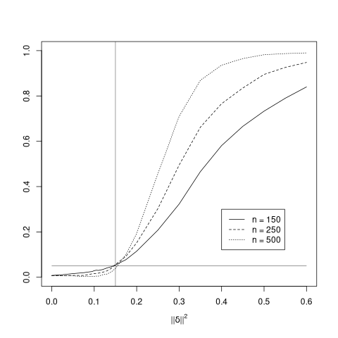
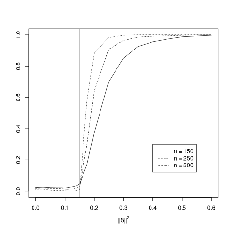
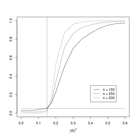
Figure 1: Empirical rejection probabilities of the test (3.9) for the hypotheses (2.2) with $\Delta=0.15$. The difference $\delta$ between the mean functions is given by (5.1) and different error processes are considered. Left panel: scaled Brownian motion (5.2); middle panel: non-seperable process in (5.3); right panel: fMA(1) process in (5.5).

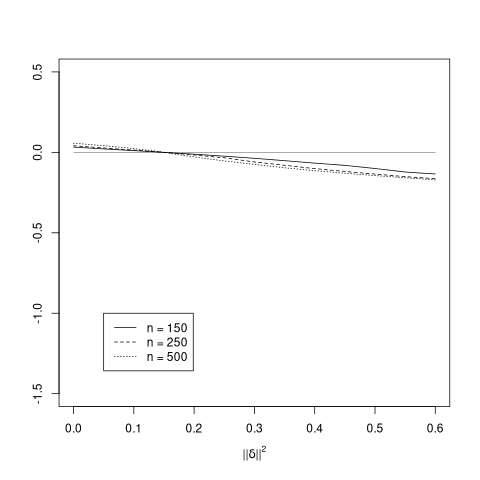
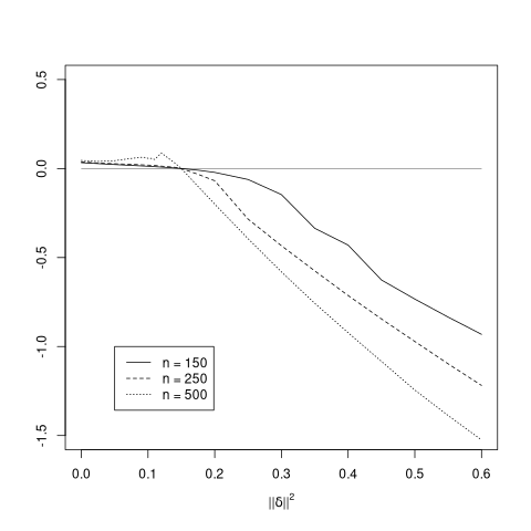
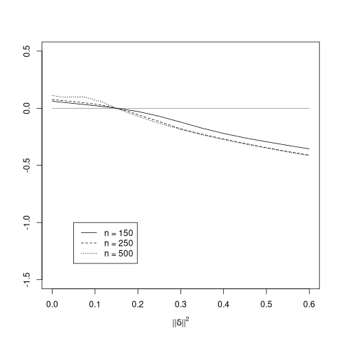
Figure 2: Size of the term $(\Delta-\left\lVert\delta\right\rVert^{2})/\tau_{\delta,\vartheta_{0}}$ as a function $\left\lVert\delta\right\rVert^{2}$ in the approximation of the rejection probability ($\Delta=0.15$) in (5.6). Left panel: scaled Brownian motion (5.2); middle panel: non-seperable process in (5.3); right panel: fMA(1) process in (5.5).

This observation can be explained by the fact that the different error processes have different variability. More precisely, it follows from the proof of Theorem 3.2 that for large sample sizes the probability of rejection can be approximated by

$$\mathrm{P}\left({\hat{\mathbb{W}}>{\sqrt{n}\over\mathbb{V}}{\Delta-\left\lVert\delta\right\rVert^{2}\over\tau_{\delta,\vartheta_{0}}}+q_{1-\alpha}(\mathbb{W})}\right)~{},$$ (5.6)

where $\tau_{\delta,\vartheta_{0}}^{2}$ is defined in (3.7) and $\mathbb{V}=\left({\int\lambda^{2}(\mathbb{B}(\lambda)-\lambda\mathbb{B}(1))^{2}\mathrm{d}\nu(\lambda)}\right)^{1/2}$ denotes a generic random variable (a functional of the Brownian motion). Thus, the power is dominated by the term $(\Delta-\left\lVert\delta\right\rVert^{2})/\tau_{\delta,\vartheta_{0}}$, which is negative under the alternative. A smaller value of this term results in a larger power and in Figure 1 we display this quantity as a function of $\|\delta\|^{2}$. The results explain the differences in the simulated power for the three processes under consideration.
We also note that the approximation of the nominal level at the boundary of the hypotheses $\|\delta\|^{2}=\Delta$ differs in the scenarios. For small sample sizes it is more accurate for the non-separable process (5.3) compared to the two other cases. A possible explanation for this observation is the different accuracy of the change point estimator (3.1) in the three scenarios, which is displayed in Figure 3. We observe that the change point estimator for the error process (5.2) exhibits a larger variability than in the two other cases, while the smallest variability is obtained for the error process (5.3).

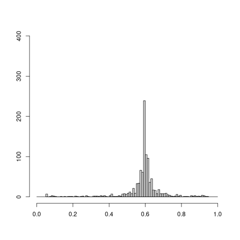
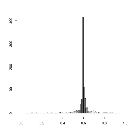
Figure 3: Histogram of the change point estimator based on $n=250$ observations. The difference between the mean functions is given by (5.1), $\Delta=0.15$, the change point is located as $\vartheta_{0}=0.6$ and different scenarios for the error process are considered. Left panel: scaled Brownian motion in (5.2); middle panel: non-separable process in (5.3); right panel: fMA(1) process in (5.5).

Next we investigate the impact of the measure $\nu$ in the self-normalizing factor (3.8) on the properties of the test (3.9). Note that this measure appears in the definition of the statistic $\hat{\mathbb{V}}_{n}$ in (3.8) and in the random variable $\mathbb{W}$ in (3.10). Thus, intuitively, there is a cancellation effect in the decision rule (3.9). For the sake of brevity, we restrict ourselves to the case of the fMA(1) error process (5.5) and display in Figure 4 the rejection probabilities of the test (3.9), where we use a uniform distribution

$$\nu_{k}=\frac{1}{k}\sum_{i=1}^{k}\delta_{i/(k+1)}$$ (5.7)

at $k=4,9$ and $k=19$ points as measure in the statistic (3.8). We observe a rather similar behaviour for all three measures, where $\nu_{19}$ yields a slightly better approximation of the nominal level at the boundary of the hypotheses (that is $\|\delta\|^{2}=\Delta=0.15$) for the sample size $n=150$.

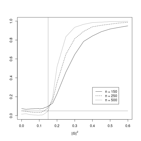
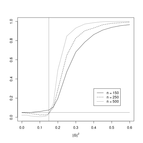
Figure 4: Empirical rejection probabilities of the test (3.9) for the hypotheses (2.2) with $\Delta=0.15$. The error process is given by an fMA(1) model and different measures in the statistic (3.8) are considered. Left panel: $\nu_{4}$, middle panel: $\nu_{9}$, right panel: $\nu_{19}$.

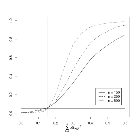
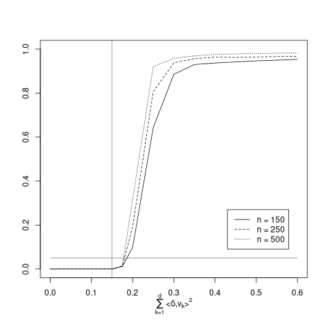
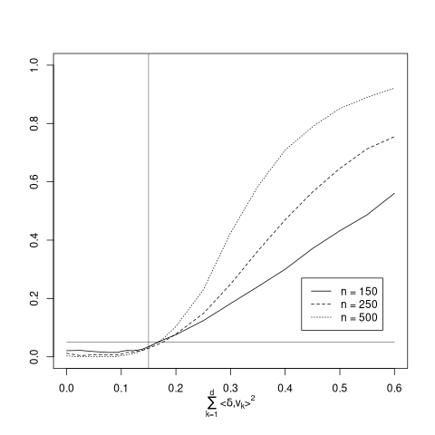
Figure 5: Empirical rejection probabilities of the test (4.11) for the hypotheses (4.2) with $\Delta=0.15$. The difference $\delta$ between the mean functions is given by (5.1) and different error processes are considered. Left panel: Brownian motion ($d=15$) ; middle panel: non-separable process ($d=11$); right panel: fMA(1) process ($d=11$).

5.1.2 Relevant changes by functional principal components

In this section, we briefly illustrate the finite sample properties of the test (4.11) for the hypotheses (4.2), where we use the same scenarios as before. The test requires the choice of the number of principal functional components and we choose the parameter $d$ such that 95% of the variance in the data will be explained. This results in $d=15$, $d=11$ and $d=11$ functional principal components for the models (5.2), (5.3) and (5.5), respectively. The corresponding rejection probabilities are displayed in Figure 5 and we observe the qualitative behaviour predicted by Theorem 4.3. We also observe that the test (4.11) is conservative in the case of the non-seperable process (5.3), while the nominal level at the boundary of the hypotheses $\sum_{k=1}^{d}\langle\delta,b_{k}\rangle^{2}=\Delta$ is very well approximated for the Brownian motion (5.2).

Finally we investigate the impact of the measure $\nu$ in the scaling factor (4.10), where we again restrict ourselves to the case of an fMA(1) process and the uniform distributions $\nu_{k}$ in (5.7) for $k=4,9$ and $19$. The corresponding results are shown in Figure 6 and demonstrate that the test (4.11) is not very sensitive with respect to this choice.

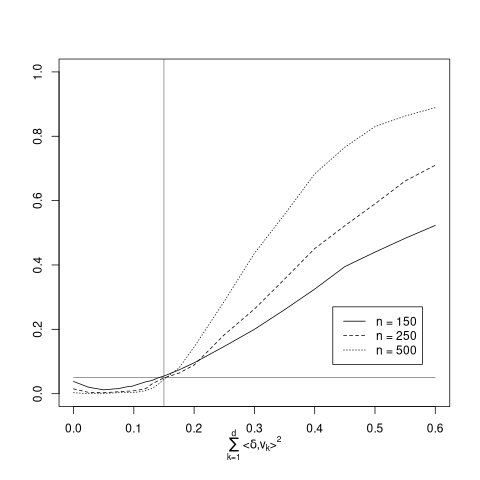
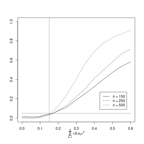
Figure 6: Empirical rejection probabilities of the test (4.11) for the hypotheses (4.2) with $\Delta=0.15$. The error process is given by an fMA(1) model and different measures in the statistic (3.8) are considered. Left panel: $\nu_{4}$, middle panel: $\nu_{9}$, right panel: $\nu_{19}$.

5.2 Data example

We conclude this paper with an application of the two test procedures in a real data example. For this purpose, we use Canadian weather data, which consists of daily measurements at $40$ representative Canadian cities. Thus we observe yearly curves at different locations over different years ($1916-2018$) at different locations. The data can be downloaded from the government of Canada website: https://climate.weather.gc.ca/historical_data/search_historic_data_e.html. The available data contains several different measurements such as maximum/minimum temperature or precipitation amount. Here, for the sake of brevity, we concentrate on the average daily temperatures. Due to missing values in the reported temperature data, four stations were chosen such that a large amount of available data overlaps and only little parts had to be interpolated or removed: Calgary International Airport, Alberta (ID: 2205), Medicine Hat Airport, Alberta (ID: 2273), Indian Head CDA, Saskatchewan (ID: 2925) and Ottawa CDA, Ontario (ID: 4333). In the notation of the previous sections this means $S=\{1,2,3,4\}$ and the sample size is given by $n=113$, which corresponds to the period from years $1891-2007$ without the years $1910,$ $1911,$ $1993$ and $1995$.

The change point estimator in (3.1) gives $\hat{\vartheta}_{n}=0.708$, which approximately corresponds to the year $1969$. We first investigate the fully functional approach in Section 3. The results of the test (3.9) for different thresholds and different nominal level are given in Table 1. We observe that $\Delta=2.974$ is the largest threshold such that the test (3.9) rejects the null hypothesis at nominal level $\alpha=0.05$. Because there are $4$ stations this corresponds to an average effect of ${2.974/4}\approx 0.74$. Finally, we note that the one-sided confidence interval $\|\delta\|\geq 0$ in (3.11) is given by $\left[{0,4.397}\right]$ while the two-sided interval $\|\delta\|>0$ in (3.12) is obtained as $\left[{0.672,4.675}\right]$

$\Delta$	10 %	5 %	1 %
2.974	reject	reject	accept
2.975	reject	accept	accept

Table 1: Results of the test (3.9) for the Canadian weather data for different nominal level and different thresholds. The value $2.974$ represents the maximal threshold (2.3), such that the null hypothesis of no relevant change is rejected at nominal level $5\%$.

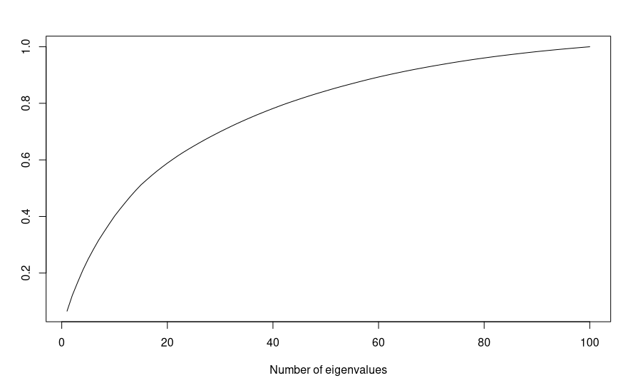
Figure 7: The function $e$ in (5.8) for $j=1,...,100$

Next we consider the test based on functional principal components developed in Section 4. In this case, the choice of $d$ is crucial and we display in Figure 7 the ratios

$$j\mapsto e(j):=\frac{\sum_{k=1}^{j}\hat{\lambda}_{k}}{{\rm trace}(\hat{c}_{\hat{\vartheta}_{n}})},$$ (5.8)

where $\hat{\lambda}_{1},\hat{\lambda}_{2},\ldots$ are the eigenvalues of the estimated covariance operator (4.1). We observe that the eigenvalues are slowly decreasing, and we choose $d=51$, which results in a value of $e(51)\approx 0.849$ of explained variance. The results of the test (4.11) for the relevant hypotheses (4.2) are shown in Table 2 for different values of $\Delta$ and $\alpha$. We observe that the maximal threshold in (4.2), such that the null hypothesis of no relevant change is rejected at nominal level $5\%$, is given by $4.467$. Finally one and two-sided confidence intervals for the quantity $\big{(}\sum_{k=1}^{d}\langle\delta,w_{k}\rangle^{2}\big{)}^{1/2}$ are obtained in same way as described in Remark 3.4 and are given by $\left[{0,3.254}\right]$ and $\left[{1.877,3.396}\right]$, respectively ($d=51$).

$\Delta$	90 %	95 %	99 %
4.467	reject	reject	accept
4.468	reject	accept	accept

Table 2: Results of the test (4.11) with $d=51$ principal components for the Canadian weather data for different nominal level and different thresholds. The value $4.467$ represents the maximal threshold in (4.2), such that the null hypothesis of no relevant change is rejected at nominal level $5\%$.

Acknowledgements This research has been supported by the German Research Foundation (DFG), project number 45723897.

Appendix A Appendix: proofs

A.1 Some preliminary results

We start with some preparations and present several results which are used in the proof. We define for $s\in S$ and $t\in\left[{0,1}\right]$

$$S_{n}(s,t,\lambda):=\frac{1}{n}\sum_{i=1}^{\lfloor\lambda n\rfloor}\left({X_{i}(s,t)-\mu(s,t)}\right)$$

and state the following result, which can be obtained by generalizing Theorem 1 in Berkes et al., (2013) to the space $L^{2}(S\times[0,1])$.

Theorem A.1.

If Assumption 2.1 is satisfied, there exists a sequence of Gaussian processes $\big{(}\left\{{\Gamma_{n}(s,t,\lambda)\mid s\in S,0\leq\lambda,t\leq 1}\right\}\big{)}_{n\in\mathbb{N}}$, such that

$$\sup_{0\leq\lambda\leq 1}\sum_{s\in S}\int\left({\sqrt{n}S_{n}(s,t,\lambda)-\Gamma_{n}(s,t,\lambda)}\right)^{2}\mathrm{d}t=\sup_{0\leq\lambda\leq 1}\left\lVert\sqrt{n}S_{n}(\cdot,\cdot,\lambda)-\Gamma_{n}(\cdot,\cdot,\lambda)\right\rVert^{2}=o_{\mathrm{P}}(1)$$

and

$$\left\{{\Gamma_{n}(s,t,\lambda)\mid s\in S,0\leq\lambda,t\leq 1}\right\}\stackrel{{\scriptstyle\text{$\mathpcal{D}$}}}{{=}}\left\{{\Gamma(s,t,\lambda)\mid s\in S,0\leq\lambda,t\leq 1}\right\},$$

where

$$\Gamma(s,t,\lambda):=\sum_{i=1}^{\infty}\sqrt{\lambda_{i}}\phi_{i}(s,t)W_{i}(\lambda),$$

$\lambda_{i},\phi_{i}$ are the eigenvalues and eigenvectors of the covariance operator of $X_{j}$ and $\{W_{i}\}_{i\in\mathbb{N}}$ are independent standard Brownian motions.

Our next auxiliary result quantifies the difference between the processes $\{D_{n}(\lambda,\vartheta_{0})\}_{\lambda\in[0,1]}$ and $\{D_{n}(\lambda,\hat{\vartheta}_{n})\}_{\lambda\in[0,1]}$ as $n\to\infty$.

Lemma A.2.

If Assumption 2.1 is satisfied, then

1. $\displaystyle\sup_{0\leq\lambda\leq 1}\left\lVert D_{n}(\lambda,\vartheta)\right\rVert=O_{\mathrm{P}}(1)$ for $\vartheta\in\{\vartheta_{0},\hat{\vartheta}_{n}\}$ ,

2. $\displaystyle\sup_{0\leq\lambda\leq 1}\left\lVert D_{n}(\lambda,\hat{\vartheta}_{n})-D_{n}(\lambda,\vartheta_{0})\right\rVert=o_{\mathrm{P}}(n^{-1/2})$.

Proof.

We can assume that $\frac{1}{n}\leq\lambda$, because, by definition, $D_{n}(\lambda,\vartheta_{0})\equiv D_{n}(\lambda,\hat{\vartheta}_{n})\equiv 0$ if $0\leq\lambda<\frac{1}{n}$, and both assertions are trivially true.

For a proof of part (1) we note that for some $\kappa>0$

$$\sup_{\frac{1}{n}\leq\lambda\leq 1}\frac{1}{\sqrt{\lfloor\lambda n\rfloor}}\left\lVert\sum_{j=1}^{\lfloor\lambda n\rfloor}\eta_{j}^{(\ell)}\right\rVert=O_{\mathrm{P}}(\log^{1/\kappa}(n))~{}~{}~{}(\ell=1,2),$$ (A.1)

which follows from Lemma B.1 in the online supplementary material of Aue et al., (2018). Let $\lambda\in\left[{1/n,1}\right]$. It suffices to show the assertion for $\vartheta=\vartheta_{0}$, because the second part of the Lemma implies the statement for $\vartheta=\hat{\vartheta}_{n}$. Then

$$\left\lVert D_{n}(\lambda,\vartheta_{0})\right\rVert\leq\left\lVert\tilde{D}_{n}(\lambda,\vartheta_{0})\right\rVert+\lambda\left\lVert\delta\right\rVert+o_{\mathrm{P}}(1)=\left\lVert\tilde{D}_{n}(\lambda,\vartheta_{0})\right\rVert+O_{\mathrm{P}}(1),$$

where the process $\{\tilde{D}_{n}(\lambda,\vartheta)\}_{\lambda\in[0,1]}$ in $L^{2}(S\times\left[{0,1}\right])$ is defined by

$$\tilde{D}_{n}(\lambda,\vartheta) :=\frac{1}{\lfloor n\vartheta\rfloor}\sum_{j=1}^{\lfloor\lambda\lfloor n\vartheta\rfloor\rfloor}\eta^{(1)}_{j}-\frac{1}{n-\lfloor n\vartheta\rfloor}\sum_{j=\lfloor n\vartheta\rfloor+1}^{\lfloor n\vartheta\rfloor+\lfloor\lambda(n-\lfloor n\vartheta\rfloor)\rfloor}\eta^{(2)}_{j}.$$

Note that $\tilde{D}_{n}(\lambda,\vartheta)$ is the centered version of ${D}_{n}(\lambda,\vartheta)$ defined in (3.3) and that

$$D_{n}(\lambda,\vartheta_{0})+\lambda\delta=\tilde{D}_{n}(\lambda,\vartheta_{0})+O_{\mathrm{P}}(n^{-1})$$ (A.2)

(note that $\vartheta_{0}\in(\varepsilon,1-\varepsilon)$ and that $\varepsilon\geq\frac{1}{n}$ if $n$ is sufficiently large). We have

$$\sup_{\frac{1}{n}\leq\lambda\leq 1}\left\lVert\tilde{D}_{n}(\lambda,\vartheta_{0})\right\rVert\leq\sup_{\frac{1}{n}\leq\lambda\leq 1}\frac{1}{\lfloor n\vartheta_{0}\rfloor}\left\lVert\sum_{j=1}^{\lfloor\lambda\lfloor n\vartheta_{0}\rfloor\rfloor}\eta_{j}^{(1)}\right\rVert+\sup_{\frac{1}{n}\leq\lambda\leq 1}\frac{1}{n-\lfloor n\vartheta_{0}\rfloor}\left\lVert\sum_{j=\lfloor n\vartheta_{0}\rfloor+1}^{\lfloor n\vartheta_{0}\rfloor+\lfloor\lambda(n-\lfloor n\vartheta_{0}\rfloor)\rfloor}\eta_{j}^{(2)}\right\rVert,$$

where the first term can be estimated as follows

$$\sup_{\frac{1}{n}\leq\lambda\leq 1}\frac{1}{\lfloor n\vartheta_{0}\rfloor}\left\lVert\sum_{j=1}^{\lfloor\lambda\lfloor n\vartheta_{0}\rfloor\rfloor}\eta_{j}^{(1)}\right\rVert \leq\frac{1}{\sqrt{\lfloor n\vartheta_{0}\rfloor}}\sup_{\frac{1}{n}\leq\lambda\leq 1}\frac{1}{\sqrt{\lfloor\lambda\lfloor n\vartheta_{0}\rfloor\rfloor}}\left\lVert\sum_{j=1}^{\lfloor\lambda\lfloor n\vartheta_{0}\rfloor\rfloor}\eta_{j}^{(1)}\right\rVert$$

$$\leq\frac{1}{\sqrt{\lfloor n\vartheta_{0}\rfloor}}\sup_{\frac{1}{n}\leq\lambda\leq 1}\frac{1}{\sqrt{\lfloor\lambda n\rfloor}}\left\lVert\sum_{j=1}^{\lfloor\lambda n\rfloor}\eta_{j}^{(1)}\right\rVert=O_{\mathrm{P}}\left({\frac{\log^{1/\kappa}(n)}{\sqrt{n}}}\right)=o_{\mathrm{P}}(1).$$

(here in the second inequality, we expanded the set over which we take the supremum and in the last step, we used the estimate (A.1)). A similar argument provides the same rate for the second term, which proves the part (1) of Lemma A.2.

For the proof of the second assertion we need the following (slightly more general) statement from the beginning of Section B.1 in Dette et al., 2020b , which states that the sequence of processes $\left\{{\Gamma_{n}(s,t,\lambda)\mid s\in S,0\leq t,\lambda\leq 1}\right\}_{n\in\mathbb{N}}$ in Theorem A.1 satisfies

$$\sup_{\begin{subarray}{c}\nu,\lambda\in\left[{0,1}\right]:\\ |\nu-\lambda|\leq\kappa_{n}\end{subarray}}\left\lVert\Gamma_{n}(\cdot,\cdot,\nu)-\Gamma_{n}(\cdot,\cdot,\lambda)\right\rVert^{2}=o_{\mathrm{P}}(1).$$ (A.3)

for any and positive sequence $\left({\kappa_{n}}\right)_{n\in\mathbb{N}}$ with $\kappa_{n}\to 0$. By adding and subtracting $\lambda\delta$, we have $D_{n}(\lambda,\hat{\vartheta}_{n})-D_{n}(\lambda,\vartheta_{0})=\tilde{D}_{n}(\lambda,\hat{\vartheta}_{n})-\tilde{D}_{n}(\lambda,\vartheta_{0})+O_{\mathrm{P}}(n^{-1})$, where

$$\tilde{D}_{n}(\lambda,\hat{\vartheta}_{n})-\tilde{D}_{n}(\lambda,\vartheta_{0}) =\frac{1}{\lfloor n\hat{\vartheta}_{n}\rfloor}\sum_{j=1}^{\lfloor\lambda\lfloor n\hat{\vartheta}_{n}\rfloor\rfloor}\eta_{j}^{(1)}-\frac{1}{\lfloor n\vartheta_{0}\rfloor}\sum_{j=1}^{\lfloor\lambda\lfloor n\vartheta_{0}\rfloor\rfloor}\eta_{j}^{(1)}$$

$$\phantom{aaa}+\frac{1}{n-\lfloor n\vartheta_{0}\rfloor}\sum_{j=\lfloor n\vartheta_{0}\rfloor+1}^{\lfloor n\vartheta_{0}\rfloor+\lfloor\lambda(n-\lfloor n\vartheta_{0}\rfloor)\rfloor}\eta_{j}^{(2)}-\frac{1}{n-\lfloor n\hat{\vartheta}_{n}\rfloor}\sum_{j=\lfloor n\hat{\vartheta}_{n}\rfloor+1}^{\lfloor n\hat{\vartheta}_{n}\rfloor+\lfloor\lambda(n-\lfloor n\hat{\vartheta}_{n}\rfloor)\rfloor}\eta_{j}^{(2)}~{}.$$

For the first difference we obtain by a similar argument as in the proof of part (1) that

$$\sup_{\frac{1}{n}\leq\lambda\leq 1}\sqrt{n}\left\lVert\frac{1}{\lfloor n\hat{\vartheta}_{n}\rfloor}\sum_{j=1}^{\lfloor\lambda\lfloor n\hat{\vartheta}_{n}\rfloor\rfloor}\eta_{j}^{(1)}-\frac{1}{\lfloor n\vartheta_{0}\rfloor}\sum_{j=1}^{\lfloor\lambda\lfloor n\vartheta_{0}\rfloor\rfloor}\eta_{j}^{(1)}\right\rVert$$

$$\phantom{aaa}\phantom{aaa}\phantom{aaa}\leq\frac{n}{\lfloor n\hat{\vartheta}_{n}\rfloor}\sup_{\frac{1}{n}\leq\lambda\leq 1}\left\lVert\frac{1}{\sqrt{n}}\sum_{j=1}^{\lfloor\lambda\lfloor n\hat{\vartheta}_{n}\rfloor\rfloor}\eta_{j}^{(1)}-\Gamma_{n}\left({\cdot,\cdot,\lambda\tfrac{\lfloor n\hat{\vartheta}_{n}\rfloor}{n}}\right)\right\rVert$$

$$\phantom{aaa}\phantom{aaa}\phantom{aaa}+\frac{n}{\lfloor n\vartheta_{0}\rfloor}\sup_{\frac{1}{n}\leq\lambda\leq 1}\left\lVert\frac{1}{\sqrt{n}}\sum_{j=1}^{\lfloor\lambda\lfloor n\vartheta_{0}\rfloor\rfloor}\eta_{j}^{(1)}-\Gamma_{n}\left({\cdot,\cdot,\lambda\tfrac{\lfloor n\vartheta_{0}\rfloor}{n}}\right)\right\rVert$$

$$\phantom{aaa}\phantom{aaa}\phantom{aaa}+\frac{n}{\lfloor n\hat{\vartheta}_{n}\rfloor}\sup_{\frac{1}{n}\leq\lambda\leq 1}\left\lVert\Gamma_{n}\left({\cdot,\cdot,\lambda\tfrac{\lfloor n\hat{\vartheta}_{n}\rfloor}{n}}\right)-\Gamma_{n}(\cdot,\cdot,\lambda\hat{\vartheta}_{n})\right\rVert$$

$$\phantom{aaa}\phantom{aaa}\phantom{aaa}+\frac{n}{\lfloor n\vartheta_{0}\rfloor}\sup_{\frac{1}{n}\leq\lambda\leq 1}\left\lVert\Gamma_{n}\left({\cdot,\cdot,\lambda\tfrac{\lfloor n\vartheta_{0}\rfloor}{n}}\right)-\Gamma_{n}(\cdot,\cdot,\lambda\vartheta_{0})\right\rVert$$

$$\phantom{aaa}\phantom{aaa}\phantom{aaa}+\sup_{\frac{1}{n}\leq\lambda\leq 1}\left\lVert\frac{n}{\lfloor n\hat{\vartheta}_{n}\rfloor}\Gamma_{n}(\cdot,\cdot,\lambda\hat{\vartheta}_{n})-\frac{n}{\lfloor n\vartheta_{0}\rfloor}\Gamma_{n}(\cdot,\cdot,\lambda\vartheta_{0})\right\rVert$$

$$\phantom{aaa}\phantom{aaa}\phantom{aaa}\leq\sup_{\begin{subarray}{c}\nu,\lambda\in\left[{0,1}\right]:\\ |\nu-\lambda|\leq\frac{1}{n}\end{subarray}}\left\lVert\Gamma_{n}(\cdot,\cdot,\nu)-\Gamma_{n}(\cdot,\cdot,\lambda)\right\rVert$$

$$\phantom{aaa}\phantom{aaa}\phantom{aaa}+O(1)\negthickspace\negthickspace\sup_{\begin{subarray}{c}\nu,\lambda\in\left[{0,1}\right]:\\ |\nu-\lambda|\leq|\hat{\vartheta}_{n}-\vartheta_{0}|\end{subarray}}\left\lVert\Gamma_{n}(\cdot,\cdot,\nu)-\Gamma_{n}(\cdot,\cdot,\lambda)\right\rVert+\frac{|\vartheta_{0}-\hat{\vartheta}_{n}|}{\vartheta_{0}\hat{\vartheta}_{n}}O_{\mathrm{P}}(1)+o_{\mathrm{P}}(1)$$

$$\phantom{aaa}\phantom{aaa}\phantom{aaa}=o_{\mathrm{P}}(1),$$

where we have used (A.3) in the last equality. Assertion (2) of Lemma A.2 now follows by a similar argument for the second difference. ∎

We conclude our preparations recalling the definition of the inner product in (4.4) and state a lemma regarding the weak convergence of the process

$$\left({{Z}_{n}^{(1)},{Z}_{n}^{(2)}}\right)^{\top} :=\big{\{}({Z}_{n}^{(1)}(\lambda),{Z}_{n}^{(2)}(\lambda))^{\top}\big{\}}_{\lambda\in[0,1]}$$ (A.4)

$$:=\Big{\{}\Big{(}\frac{1}{\sqrt{n}}\sum_{i=1}^{\lfloor n\lambda\rfloor}\left({\langle\eta_{i}^{(k)}\otimes\eta_{i}^{(k)}-c^{(k)}{},\xi_{k}\rangle_{2}+\langle\eta_{i}^{(k)},\zeta_{k}\rangle}\right)\Big{)}_{k=1,2}\Big{\}}_{\lambda\in[0,1]}~{},$$

where $\{\eta^{(1)}_{j}\}_{j\in\mathbb{Z}}$ and $\{\eta^{(2)}_{j}\}_{j\in\mathbb{Z}}$ are centered processes in $L^{2}(S\times\left[{0,1}\right])$ and $\zeta_{1},\zeta_{2}\in L^{2}(S\times\left[{0,1}\right])$, $\xi_{1},\xi_{2}\in L^{2}((S\times\left[{0,1}\right])^{2})$ are given functions. We emphasize that we consider the process $({Z}_{n}^{(1)},{Z}_{n}^{(2)})^{\top}$ with different parameters $\zeta_{1},\zeta_{2}\in L^{2}(S\times\left[{0,1}\right])$, $\xi_{1},\xi_{2}\in L^{2}((S\times\left[{0,1}\right])^{2})$ in the proofs of the results of Section 3 and 4. The proof of the following result is similar to the proof of Lemma B.1 in Dette et al., 2020b and therefore omitted.

Lemma A.3.

Let $\zeta_{1},\zeta_{2}\in L^{2}(S\times\left[{0,1}\right])$, $\xi_{1},\xi_{2}\in L^{2}((S\times\left[{0,1}\right])^{2})$ be fixed but arbitrary functions and let $\{\eta^{(1)}_{j}\}_{j\in\mathbb{Z}},$ $\{\eta^{(2)}_{j}\}_{j\in\mathbb{Z}}$ denote centered processes satisfying Assumption 4.1. Then the process defined in (A.4) converges weakly in $\ell^{\infty}(\left[{0,1}\right])^{2}$, that is

$$\left({{Z}_{n}^{(1)},{Z}_{n}^{(2)}}\right)^{\top}\rightsquigarrow\Sigma^{1/2}\left({\mathbb{B}_{1},\mathbb{B}_{2}}\right)^{\top},$$ (A.5)

where $\mathbb{B}_{1},\mathbb{B}_{2}$ are independent Brownian motions and $\Sigma=(\Sigma_{kl})_{k,l=1,2}$ is a $2\times 2$ matrix with entries

$$\Sigma_{kl}=\sum_{i\in\mathbb{Z}} \bigg{(}\mathrm{Cov}(\langle\eta_{0}^{(k)}\otimes\eta_{0}^{(k)},\xi_{k}\rangle_{2},\langle\eta_{i}^{(l)}\otimes\eta_{i}^{(l)},\xi_{l}\rangle_{2})+\mathrm{Cov}(\langle\eta_{0}^{(k)}\otimes\eta_{0}^{(k)},\xi_{k}\rangle_{2},\langle\eta_{i}^{(l)},\zeta_{l}\rangle)$$

$$\phantom{a}+\mathrm{Cov}(\langle\eta_{0}^{(k)},\zeta_{k}\rangle,\langle\eta_{i}^{(l)}\otimes\eta_{i}^{(l)},\xi_{l}\rangle_{2})+\mathrm{Cov}(\langle\eta_{0}^{(k)},\zeta_{k}\rangle,\langle\eta_{i}^{(l)},\zeta_{l}\rangle)\bigg{)}.$$ (A.6)

Moreover, in the case $\xi_{1}\equiv\xi_{2}\equiv 0$ Assumption 2.1 instead of Assumption 4.1 is sufficient for the weak convergence in (A.5).

A.2 Proof of Theorem 3.1

For a proof of the weak convergence in (3.5) we use (A.2) and several applications of the Cauchy-Schwarz inequality, which give

$$\mathbb{U}_{n}(\lambda) :=\sqrt{n}\left({\left\lVert D_{n}(\lambda,\vartheta_{0})\right\rVert^{2}-\lambda^{2}\left\lVert\delta\right\rVert^{2}}\right)=\tfrac{1}{\sqrt{n}}\left\lVert\sqrt{n}\tilde{D}_{n}(\lambda,\vartheta_{0})\right\rVert^{2}+2\lambda\langle\sqrt{n}\tilde{D}_{n}(\lambda,\vartheta_{0}),\delta\rangle+o_{\mathrm{P}}(1)$$

$$=2\lambda\langle\sqrt{n}\tilde{D}_{n}(\lambda,\vartheta_{0}),\delta\rangle+o_{\mathrm{P}}(1),$$

since $\left\lVert\sqrt{n}\tilde{D}_{n}(\lambda,\vartheta_{0})\right\rVert^{2}=O_{\mathrm{P}}(1)$ by Theorem A.1. Next define for $\ell=1,2$ and $\lambda\in\left[{0,1}\right]$

$${Z}^{(\ell)}_{n}(\lambda):=\frac{1}{\sqrt{n}}\sum_{j=1}^{\lfloor\lambda n\rfloor}\langle\eta_{j}^{(\ell)},\delta\rangle,$$

in order to rewrite

$$\langle\sqrt{n}\tilde{D}_{n}(\lambda,\vartheta_{0}),\delta\rangle =\frac{n}{\lfloor n\vartheta_{0}\rfloor}\frac{1}{\sqrt{n}}\sum_{i=1}^{\lfloor\lambda\lfloor n\vartheta_{0}\rfloor\rfloor}\langle\eta_{i}^{(1)},\delta\rangle-\frac{n}{n-\lfloor n\vartheta_{0}\rfloor}\frac{1}{\sqrt{n}}\sum_{i=\lfloor n\vartheta_{0}\rfloor+1}^{\lfloor n\vartheta_{0}\rfloor+\lambda(n-\lfloor n\vartheta_{0}\rfloor)}\langle\eta_{i}^{(2)},\delta\rangle$$

$$=\frac{n}{\lfloor n\vartheta_{0}\rfloor}{Z}^{(1)}_{n}\left({\lambda\tfrac{\lfloor n\vartheta_{0}\rfloor}{n}}\right)-\frac{n}{n-\lfloor n\vartheta_{0}\rfloor}\left({{Z}^{(2)}_{n}\left({\tfrac{\lfloor n\vartheta_{0}\rfloor+\lfloor\lambda(n-\lfloor n\vartheta_{0}\rfloor)\rfloor}{n}}\right)-{Z}^{(2)}_{n}\left({\vartheta_{0}}\right)}\right).$$

Hence,

$$\mathbb{U}_{n}(\lambda) =\sqrt{n}\left({\left\lVert D_{n}(\lambda,\vartheta_{0})\right\rVert^{2}-\lambda^{2}\left\lVert\delta\right\rVert^{2}}\right)$$

$$=\frac{2\lambda}{\vartheta_{0}}{Z}^{(1)}_{n}\left({\lambda\tfrac{\lfloor n\vartheta_{0}\rfloor}{n}}\right)-\frac{2\lambda}{1-\vartheta_{0}}\left({{Z}^{(2)}_{n}\left({\tfrac{\lfloor n\vartheta_{0}\rfloor+\lfloor\lambda(n-\lfloor n\vartheta_{0}\rfloor)\rfloor}{n}}\right)-{Z}^{(2)}_{n}\left({\vartheta_{0}}\right)}\right)+o_{\mathrm{P}}(1)$$

and by an application of Lemma A.3 with $\zeta_{1}=\zeta_{2}=\delta$ and $\xi_{1}\equiv\xi_{2}\equiv 0$, (note that in this case Assumption 2.1 is sufficient) we obtain

$$\left\{{\mathbb{U}_{n}(\lambda)}\right\}_{\lambda\in\left[{0,1}\right]}\rightsquigarrow \left\{{\mathbb{Z}(\lambda)}\right\}_{\lambda\in\left[{0,1}\right]}$$

$$:=\left\{{\frac{2\lambda}{\vartheta_{0}}{\mathbb{Z}}^{(1)}(\lambda\vartheta_{0})-\frac{2\lambda}{1-\vartheta_{0}}\left({{\mathbb{Z}}^{(2)}(\vartheta_{0}+\lambda(1-\vartheta_{0}))-{\mathbb{Z}}^{(2)}(\vartheta_{0})}\right)}\right\}_{\lambda\in\left[{0,1}\right]},$$

with ${\mathbb{Z}}^{(1)}={\Sigma}_{11}^{*}\mathbb{B}_{1}+{{\Sigma}}_{12}^{*}\mathbb{B}_{2}$ and ${\mathbb{Z}}^{(2)}={\Sigma}_{21}^{*}\mathbb{B}_{1}+{\Sigma}_{22}^{*}\mathbb{B}_{2},$ where $\mathbb{B}_{1}$ and $\mathbb{B}_{2}$ are independent Brownian motions. Here ${\Sigma}_{ij}^{*}$ denotes the $ij$-th entry of the matrix $\Sigma^{1/2}$ ($i,j=1,2$) and $\Sigma$ is defined by the entries given in (A.6), where in this case $\zeta_{1}=\zeta_{2}=\delta$ and $\xi_{1}\equiv\xi_{2}\equiv 0$. Inspecting the covariance structure of the limit above, we see that because of

$$\mathrm{Cov}({\mathbb{Z}}^{(1)}(\lambda_{1}\vartheta_{0}),{\mathbb{Z}}^{(1)}(\lambda_{2}\vartheta_{0})) =(\lambda_{1}\wedge\lambda_{2})\vartheta_{0}\Sigma_{11},$$

$$\mathrm{Cov}({\mathbb{Z}}^{(2)}(\vartheta_{0}+\lambda_{1}(1-\vartheta_{0}))-{\mathbb{Z}}^{(2)}(\vartheta_{0}),{\mathbb{Z}}^{(2)}(\vartheta_{0}+\lambda_{2}(1-\vartheta_{0}))-{\mathbb{Z}}^{(2)}(\vartheta_{0})) =(\lambda_{1}\wedge\lambda_{2})(1-\vartheta_{0})\Sigma_{22},$$

$$\mathrm{Cov}({\mathbb{Z}}^{(1)}(\lambda_{1}\vartheta_{0}),{\mathbb{Z}}^{(2)}(\vartheta_{0}+\lambda_{2}(1-\vartheta_{0}))-{\mathbb{Z}}^{(2)}(\vartheta_{0})) =0,$$

we have

$$\mathrm{Cov}\left({\mathbb{Z}(\lambda_{2}),\mathbb{Z}(\lambda_{2})}\right)=4\lambda_{1}\lambda_{2}(\lambda_{1}\wedge\lambda_{2})\left({\frac{1}{\vartheta_{0}}\Sigma_{11}+\frac{1}{1-\vartheta_{0}}\Sigma_{22}}\right).$$

Hence the limit has the same distribution as $\tau_{\delta,\vartheta_{0}}\left\{{\lambda\mathbb{B}(\lambda)}\right\}_{\lambda\in\left[{0,1}\right]}$, and the first assertion follows.

For a proof of (3.6), we rewrite the expression as

$$\sqrt{n}\left({\left\lVert D_{n}(\lambda,\hat{\vartheta}_{n})\right\rVert^{2}-\lambda^{2}\left\lVert\delta\right\rVert^{2}}\right) =\sqrt{n}\big{(}\left\lVert D_{n}(\lambda,{\vartheta_{0}})\right\rVert^{2}-\lambda^{2}\left\lVert\delta\right\rVert^{2}\big{)}+N_{n}(\lambda),$$

where

$$N_{n}(\lambda):=\sqrt{n}\bigg{(}\left\lVert D_{n}(\lambda,\hat{\vartheta}_{n})-D_{n}(\lambda,{\vartheta_{0}})\right\rVert^{2}+2\langle D_{n}(\lambda,\hat{\vartheta}_{n}),D_{n}(\lambda,\hat{\vartheta}_{n})-D_{n}(\lambda,{\vartheta_{0}})\rangle\bigg{)}$$

By the Cauchy-Schwarz inequality and both parts of Lemma A.2, we obtain $\sup_{\lambda}N_{n}(\lambda)=o_{\mathrm{P}}(1)$. Therefore, the convergence follows from (3.5).

A.3 Proof of Theorem 3.2

First of all, we consider $\|\delta\|^{2}=0$. By a careful inspection of the proof part 1 of Lemma A.2, we can verify that $\hat{\mathbb{D}}_{n}$ is a consistent estimator of $\|\delta\|^{2}$. So in this case, we have $\hat{\mathbb{D}}_{n}=o_{\mathrm{P}}(1)$. By Remark 3.3 the random variable $\mathbb{W}$ in (3.10) has a symmetric distribution, which in turn implies $q_{1-\alpha}(\mathbb{W})\geq 0$, whenever $\alpha\leq 0.5$. Together with the fact that $\hat{\mathbb{V}}_{n}\geq 0$, we have

$$\mathrm{P}\left({\hat{\mathbb{D}}_{n}>\Delta+q_{1-\alpha}(\mathbb{W})\hat{\mathbb{V}}_{n}}\right)\longrightarrow 0,$$

whenever $\Delta>0$ and $\alpha\leq 0.5$. Now, consider the case $\|\delta\|>0$, then, by Theorem 3.1, the weak convergence of the vector $\sqrt{n}\big{(}(\hat{\mathbb{D}}_{n}-\left\lVert\delta\right\rVert^{2}),\hat{\mathbb{V}}_{n}\big{)}^{\top}$ is an immediate consequence of (3.6) and the continuous mapping theorem applied to the map

$$f\longmapsto\big{(}f(1),\big{(}\int_{0}^{1}\lambda^{2}(f(\lambda)-\lambda f(1))\mathrm{d}\nu(\lambda)\big{)}^{1/2}\big{)}^{\top}.$$

Hence, we have $\hat{\mathbb{D}}_{n}-\left\lVert\delta\right\rVert^{2}=o_{\mathrm{P}}(1)$ and $\hat{\mathbb{V}}_{n}=o_{\mathrm{P}}(1)$. Therefore,

$$\mathrm{P}\left({\hat{\mathbb{D}}_{n}-\left\lVert\delta\right\rVert^{2}>\Delta-\left\lVert\delta\right\rVert^{2}+q_{1-\alpha}(\mathbb{W})\hat{\mathbb{V}}_{n}}\right)\longrightarrow\begin{cases}0,&\text{if }\left\lVert\delta\right\rVert^{2}<\Delta,\\ 1,&\text{if }\left\lVert\delta\right\rVert^{2}>\Delta,\end{cases}$$

as $n\to\infty$. In the case $\left\lVert\delta\right\rVert^{2}=\Delta$ and $\tau_{\delta,\vartheta_{0}}^{2}>0$, we obtain from (3.6) and the continuous mapping theorem applied to the map $f\longmapsto f(1)\big{(}\int_{0}^{1}\lambda^{2}(f(\lambda)-\lambda f(1))\mathrm{d}\nu(\lambda)\big{)}^{-1/2}$, that

$$\frac{\hat{\mathbb{D}}_{n}-\left\lVert\delta\right\rVert^{2}}{\hat{\mathbb{V}}_{n}}\rightsquigarrow\mathbb{W},$$

where $\mathbb{W}$ is defined in (3.10). This yields

$$\lim_{n\to\infty}\mathrm{P}\left({\hat{\mathbb{D}}_{n}>\Delta+q_{1-\alpha}(\mathbb{W})\hat{\mathbb{V}}_{n}}\right)=\lim_{n\to\infty}\mathrm{P}\left({\frac{\hat{\mathbb{D}}_{n}-\left\lVert\delta\right\rVert^{2}}{\hat{\mathbb{V}}_{n}}>q_{1-\alpha}(\mathbb{W})}\right)=\alpha.$$

A.4 Proof of Theorem 4.1

We show that

$$\sup_{0\leq\lambda\leq 1}\sqrt{\lambda}\left\lVert\hat{\vartheta}_{n}\hat{c}^{(1)}_{\lambda}-\vartheta_{0}\mathrm{E}\left[{\eta_{0}^{(1)}\otimes\eta_{0}^{(1)}}\right]\right\rVert_{2} =O_{\mathrm{P}}\left({\frac{\log^{2/\kappa}(n)}{\sqrt{n}}}\right)~{},$$ (A.7)

$$\sup_{0\leq\lambda\leq 1}\sqrt{\lambda}\left\lVert(1-\hat{\vartheta}_{n})\hat{c}_{\lambda}^{(2)}-(1-\vartheta_{0})\mathrm{E}\left[{\eta_{0}^{(2)}\otimes\eta_{0}^{(2)}}\right]\right\rVert_{2} =O_{\mathrm{P}}\left({\frac{\log^{2/\kappa}(n)}{\sqrt{n}}}\right)~{},$$ (A.8)

For the sake of brevity we restrict ourselves to a proof of (A.7), the proof of (A.8) follows by similar arguments.

First, we assume that $\lambda<\frac{1}{\lfloor n\hat{\vartheta}_{n}\rfloor}$, then $\hat{c}^{(1)}_{\lambda}=0$ and

$$\sqrt{\lambda}\left\lVert\hat{\vartheta}_{n}\hat{c}^{(1)}_{\lambda}-\vartheta_{0}\mathrm{E}\left[{\eta_{0}^{(1)}\otimes\eta_{0}^{(1)}}\right]\right\rVert_{2}<\frac{\vartheta_{0}}{\sqrt{\lfloor n\hat{\vartheta}_{n}\rfloor}}\bigg{|}\mathrm{E}\left[{\eta_{0}^{(1)}\otimes\eta_{0}^{(1)}}\right]\bigg{|}=O_{\mathrm{P}}(n^{-1/2})$$

uniformly in $\lambda\in[0,\frac{1}{\lfloor n\hat{\vartheta}_{n}\rfloor})$. If $\frac{1}{\lfloor n\hat{\vartheta}_{n}\rfloor}\leq\lambda\leq 1$ we use the representation

$$\hat{c}^{(1)}_{\lambda}=\frac{1}{\lfloor\lambda\lfloor n\hat{\vartheta}_{n}\rfloor\rfloor}\sum_{i=1}^{\lfloor\lambda\lfloor n\hat{\vartheta}_{n}\rfloor\rfloor}X_{i}\otimes X_{i}-\frac{1}{\lfloor\lambda\lfloor n\hat{\vartheta}_{n}\rfloor\rfloor^{2}}\sum_{i,j=1}^{\lfloor\lambda\lfloor n\hat{\vartheta}_{n}\rfloor\rfloor}X_{i}\otimes X_{j}$$ (A.9)

and consider the first term. For this we get

$$\frac{1}{\lfloor\lambda\lfloor n\hat{\vartheta}_{n}\rfloor\rfloor}\sum_{i=1}^{\lfloor\lambda\lfloor n\hat{\vartheta}_{n}\rfloor\rfloor}X_{i}\otimes X_{i}=\frac{1}{\lfloor\lambda\lfloor n\hat{\vartheta}_{n}\rfloor\rfloor}\sum_{i=1}^{\lfloor\lambda\lfloor n\hat{\vartheta}_{n}\rfloor\rfloor\wedge\lfloor n\vartheta_{0}\rfloor}X_{i}\otimes X_{i}$$

$$~{}~{}~{}~{}~{}~{}~{}~{}~{}~{}~{}~{}~{}~{}~{}~{}~{}~{}~{}~{}~{}~{}~{}~{}~{}~{}~{}~{}~{}~{}~{}~{}~{}~{}~{}~{}~{}~{}~{}~{}~{}~{}~{}~{}~{}~{}~{}~{}~{}~{}~{}~{}~{}~{}+\frac{1}{\lfloor\lambda\lfloor n\hat{\vartheta}_{n}\rfloor\rfloor}\sum_{i=\lfloor\lambda\lfloor n\hat{\vartheta}_{n}\rfloor\rfloor\wedge\lfloor n\vartheta_{0}\rfloor+1}^{\lfloor\lambda\lfloor n\hat{\vartheta}_{n}\rfloor\rfloor}X_{i}\otimes X_{i}$$

$$~{}~{}~{}~{}~{}~{}~{}~{}~{}~{}~{}~{}=\frac{1}{\lfloor\lambda\lfloor n\hat{\vartheta}_{n}\rfloor\rfloor}\sum_{i=1}^{\lfloor\lambda\lfloor n\hat{\vartheta}_{n}\rfloor\rfloor\wedge\lfloor n\vartheta_{0}\rfloor}\left({\eta_{i}^{(1)}\otimes\eta_{i}^{(1)}+\mu\otimes\eta_{i}^{(1)}+\eta_{i}^{(1)}\otimes\mu+\mu\otimes\mu}\right)$$

$$~{}~{}~{}~{}~{}~{}~{}~{}~{}~{}~{}~{}+\frac{1}{\lfloor\lambda\lfloor n\hat{\vartheta}_{n}\rfloor\rfloor}\sum_{i=\lfloor\lambda\lfloor n\hat{\vartheta}_{n}\rfloor\rfloor\wedge\lfloor n\vartheta_{0}\rfloor+1}^{\lfloor\lambda\lfloor n\hat{\vartheta}_{n}\rfloor\rfloor}\left({\eta_{i}^{(2)}\otimes\eta_{i}^{(2)}+\tilde{\mu}\otimes\eta_{i}^{(2)}+\eta_{i}^{(2)}\otimes\tilde{\mu}+\tilde{\mu}\otimes\tilde{\mu}}\right),$$ (A.10)

where we use the notation $\tilde{\mu}:=\mu+\delta$. The second term in (A.9) can be rewritten as follows:

$$\frac{1}{\lfloor\lambda\lfloor n\hat{\vartheta}_{n}\rfloor\rfloor^{2}} \sum_{i,j=1}^{\lfloor\lambda\lfloor n\hat{\vartheta}_{n}\rfloor\rfloor}X_{i}\otimes X_{j}$$

$$=\frac{1}{\lfloor\lambda\lfloor n\hat{\vartheta}_{n}\rfloor\rfloor^{2}}\sum_{i,j=1}^{\lfloor\lambda\lfloor n\hat{\vartheta}_{n}\rfloor\rfloor\wedge\lfloor n\vartheta_{0}\rfloor}\left({\eta_{i}^{(1)}\otimes\eta_{j}^{(1)}+\mu\otimes\eta_{j}^{(1)}+\eta_{i}^{(1)}\otimes\mu+\mu\otimes\mu}\right)$$

$$+\frac{\mathbbm{1}\left\{{\lfloor n\vartheta_{0}\rfloor\leq\lfloor\lambda\lfloor n\hat{\vartheta}_{n}\rfloor\rfloor}\right\}}{\lfloor\lambda\lfloor n\hat{\vartheta}_{n}\rfloor\rfloor^{2}}\bigg{[}\sum_{i=1}^{\lfloor n\vartheta_{0}\rfloor}\sum_{j=\lfloor n\vartheta_{0}\rfloor+1}^{\lfloor\lambda\lfloor n\hat{\vartheta}_{n}\rfloor\rfloor}\left({\eta_{i}^{(1)}\otimes\eta_{j}^{(2)}+\mu\otimes\eta_{j}^{(2)}+\eta_{i}^{(1)}\otimes\tilde{\mu}+\mu\otimes\tilde{\mu}}\right)$$

$$\phantom{asdfasdfasdasdfsdfa}+\sum_{i=\lfloor n\vartheta_{0}\rfloor+1}^{\lfloor\lambda\lfloor n\hat{\vartheta}_{n}\rfloor\rfloor}\sum_{j=1}^{\lfloor n\vartheta_{0}\rfloor}\left({\eta_{i}^{(2)}\otimes\eta_{j}^{(1)}+\eta_{i}^{(2)}\otimes\mu+\tilde{\mu}\otimes\eta_{j}^{(1)}+\tilde{\mu}\otimes\mu}\right)$$

$$\phantom{asdfasdfaasdsdfsdfa}+\sum_{i,j=\lfloor n\vartheta_{0}\rfloor+1}^{\lfloor\lambda\lfloor n\hat{\vartheta}_{n}\rfloor\rfloor}\left({\eta_{i}^{(2)}\otimes\eta_{j}^{(2)}+\eta_{i}^{(2)}\otimes\tilde{\mu}+\tilde{\mu}\otimes\eta_{j}^{(2)}+\tilde{\mu}\otimes\tilde{\mu}}\right)\bigg{]}.$$

We now consider the cases $\lfloor\lambda\lfloor n\hat{\vartheta}_{n}\rfloor\rfloor<\lfloor n\vartheta_{0}\rfloor$ and $\lfloor\lambda\lfloor n\hat{\vartheta}_{n}\rfloor\rfloor\geq\lfloor n\vartheta_{0}\rfloor$ separately. For this purpose, we define the set $\Lambda:=\{\frac{1}{\lfloor n\hat{\vartheta}_{n}\rfloor}\leq\lambda\leq 1\mid\lfloor\lambda\lfloor n\hat{\vartheta}_{n}\rfloor\rfloor<\lfloor n\vartheta_{0}\rfloor\}$ and note that

$$\sup_{\frac{1}{n}\leq\lambda\leq 1}\sqrt{\lambda}\left\lVert\hat{\vartheta}_{n}\hat{c}_{\lambda}^{(1)}-\vartheta_{0}\mathrm{E}\left[{\eta_{0}^{(1)}\otimes\eta_{0}^{(1)}}\right]\right\rVert_{2}$$

$$\phantom{aaa}=\max\left\{{\sup_{\lambda\in\Lambda}\sqrt{\lambda}\left\lVert\hat{\vartheta}_{n}\hat{c}_{\lambda}^{(1)}-\vartheta_{0}\mathrm{E}\left[{\eta_{0}^{(1)}\otimes\eta_{0}^{(1)}}\right]\right\rVert_{2},\sup_{\lambda\in\Lambda^{C}}\sqrt{\lambda}\left\lVert\hat{\vartheta}_{n}\hat{c}_{\lambda}^{(1)}-\vartheta_{0}\mathrm{E}\left[{\eta_{0}^{(1)}\otimes\eta_{0}^{(1)}}\right]\right\rVert_{2}}\right\}~{}.$$

We consider each case individually, starting with the first term, where the $\sup$ is taken over the set $\Lambda$, i.e. $\lfloor\lambda\lfloor n\hat{\vartheta}_{n}\rfloor\rfloor<\lfloor n\vartheta_{0}\rfloor$. Observing that the sum in (A.10) vanishes, we obtain in this case that

$$\hat{c}_{\lambda}^{(1)}=\frac{1}{\lfloor\lambda\lfloor n\hat{\vartheta}_{n}\rfloor\rfloor}\sum_{i=1}^{\lfloor\lambda\lfloor n\hat{\vartheta}_{n}\rfloor\rfloor}\eta_{i}^{(1)}\otimes\eta_{i}^{(1)}-\frac{1}{\lfloor\lambda\lfloor n\hat{\vartheta}_{n}\rfloor\rfloor^{2}}\sum_{i,j=1}^{\lfloor\lambda\lfloor n\hat{\vartheta}_{n}\rfloor\rfloor}\eta_{i}^{(1)}\otimes\eta_{j}^{(1)}$$ (A.11)

In the subsequent discussion, we will repeatedly make use of the following inequality, without explicitly mentioning it. It is obtained by expanding the set over which the supremum is calculated, and substituting $\lambda^{\prime}=\lambda\frac{\lfloor n\hat{\vartheta}_{n}\rfloor}{n}$:

$$\sup_{\lambda\in\Lambda}\frac{1}{\sqrt{\lfloor\lambda\lfloor n\hat{\vartheta}_{n}\rfloor\rfloor}}\left\lVert\sum_{i=1}^{\lfloor\lambda\lfloor n\hat{\vartheta}_{n}\rfloor\rfloor}\eta_{i}^{(1)}\right\rVert \leq\sup_{\frac{1}{n}\leq\lambda^{\prime}\leq\frac{\lfloor n\hat{\vartheta}_{n}\rfloor}{n}}\frac{1}{\sqrt{\lfloor\lambda^{\prime}n\rfloor}}\left\lVert\sum_{i=1}^{\lfloor\lambda^{\prime}n\rfloor}\eta_{i}^{(1)}\right\rVert\leq\sup_{\frac{1}{n}\leq\lambda\leq 1}\frac{1}{\sqrt{\lfloor\lambda n\rfloor}}\left\lVert\sum_{i=1}^{\lfloor\lambda n\rfloor}\eta_{i}^{(1)}\right\rVert.$$

Regarding the second term in (A.11) we have for some $\kappa>0$

$$\sup_{\lambda\in\Lambda}\sqrt{\lambda}\hat{\vartheta}_{n}\left\lVert\frac{1}{\lfloor\lambda\lfloor n\hat{\vartheta}_{n}\rfloor\rfloor^{2}}\sum_{i,j=1}^{\lfloor\lambda\lfloor n\hat{\vartheta}_{n}\rfloor\rfloor}\eta_{i}^{(1)}\otimes\eta_{j}^{(1)}\right\rVert_{2} =\sup_{\lambda\in\Lambda}\frac{\lambda\hat{\vartheta}_{n}}{\lfloor\lambda\lfloor n\hat{\vartheta}_{n}\rfloor\rfloor}\frac{1}{\sqrt{\lambda}}\left\lVert\frac{1}{\sqrt{\lfloor\lambda\lfloor n\hat{\vartheta}_{n}\rfloor\rfloor}}\sum_{i=1}^{\lfloor\lambda\lfloor n\hat{\vartheta}_{n}\rfloor\rfloor}\eta_{i}^{(1)}\right\rVert^{2}$$

$$\leq O_{\mathrm{P}}(n^{-1/2})\left({\sup_{\frac{1}{n}\leq\lambda\leq 1}\frac{1}{\sqrt{\lfloor\lambda n\rfloor}}\left\lVert\sum_{i=1}^{\lfloor\lambda n\rfloor}\eta_{i}^{(1)}\right\rVert}\right)^{2}$$

$$=O_{\mathrm{P}}\left({\frac{\log^{2/\kappa}(n)}{\sqrt{n}}}\right),$$

by (A.1). This implies

$$\sup_{\lambda\in\Lambda}\sqrt{\lambda}\left\lVert\hat{\vartheta}_{n}\hat{c}_{\lambda}^{(1)}-\vartheta_{0}\mathrm{E}\left[{\eta_{0}^{(1)}\otimes\eta_{0}^{(1)}}\right]\right\rVert_{2}$$

$$~{}~{}~{}~{}~{}~{}~{}~{}\leq\sup_{\lambda\in\Lambda}\sqrt{\lambda}\left\lVert\frac{\hat{\vartheta}_{n}}{\lfloor\lambda\lfloor n\hat{\vartheta}_{n}\rfloor\rfloor}\sum_{i=1}^{\lfloor\lambda\lfloor n\hat{\vartheta}_{n}\rfloor\rfloor}\left({\eta_{i}^{(1)}\otimes\eta_{i}^{(1)}-\mathrm{E}\left[{\eta_{0}^{(1)}\otimes\eta_{0}^{(1)}}\right]}\right)\right\rVert_{2}$$

$$\phantom{aaa}\phantom{aaa}~{}~{}~{}~{}~{}~{}~{}~{}~{}~{}~{}~{}~{}~{}~{}~{}+|\hat{\vartheta}_{n}-\vartheta_{0}|\mathrm{E}\left[{\eta_{0}^{(1)}\otimes\eta_{0}^{(1)}}\right]+O_{\mathrm{P}}\left({\frac{\log^{2/\kappa}(n)}{\sqrt{n}}}\right)$$

$$~{}~{}~{}~{}~{}~{}~{}~{}\leq O_{\mathrm{P}}(n^{-1/2})\sup_{\frac{1}{n}\leq\lambda\leq 1}\frac{1}{\sqrt{\lfloor\lambda n\rfloor}}\left\lVert\sum_{i=1}^{\lfloor\lambda n\rfloor}\left({\eta_{i}^{(1)}\otimes\eta_{i}^{(1)}-\mathrm{E}\left[{\eta_{0}^{(1)}\otimes\eta_{0}^{(1)}}\right]}\right)\right\rVert_{2}+O_{\mathrm{P}}\left({\frac{\log^{2/\kappa}(n)}{\sqrt{n}}}\right)$$

$$~{}~{}~{}~{}~{}~{}~{}~{}\leq O_{\mathrm{P}}\left({\frac{\log^{2/\kappa}(n)}{\sqrt{n}}}\right),$$

where we used (3.2) and again a variation of (A.1), this time for $L^{2}((S\times\left[{0,1}\right])^{2})$-valued random variables.

It remains to calculate the supremum over the set $\Lambda^{C}$. If $\lfloor\lambda\lfloor n\hat{\vartheta}_{n}\rfloor\rfloor\geq\lfloor n\vartheta_{0}\rfloor$, a tedious but straightforward calculation gives

$$\hat{c}_{\lambda}^{(1)} =\frac{1}{\lfloor\lambda\lfloor n\hat{\vartheta}_{n}\rfloor\rfloor}\sum_{i=1}^{\lfloor n\vartheta_{0}\rfloor}\eta_{i}^{(1)}\otimes\eta_{i}^{(1)}-\frac{1}{\lfloor\lambda\lfloor n\hat{\vartheta}_{n}\rfloor\rfloor^{2}}\sum_{i,j=1}^{\lfloor n\vartheta_{0}\rfloor}\eta_{i}^{(1)}\otimes\eta_{j}^{(1)}$$

$$\phantom{aa}+\frac{1}{\lfloor\lambda\lfloor n\hat{\vartheta}_{n}\rfloor\rfloor}\sum_{i=\lfloor n\vartheta_{0}\rfloor+1}^{\lfloor\lambda\lfloor n\hat{\vartheta}_{n}\rfloor\rfloor}(\eta_{i}^{(2)}+\delta)\otimes(\eta_{i}^{(2)}+\delta)$$

$$\phantom{aa}-\frac{1}{\lfloor\lambda\lfloor n\hat{\vartheta}_{n}\rfloor\rfloor^{2}}\sum_{i=1}^{\lfloor n\vartheta_{0}\rfloor}\sum_{j=\lfloor n\vartheta_{0}\rfloor+1}^{\lfloor\lambda\lfloor n\hat{\vartheta}_{n}\rfloor\rfloor}\eta_{i}^{(1)}\otimes(\eta_{j}^{(2)}+\delta)-\frac{1}{\lfloor\lambda\lfloor n\hat{\vartheta}_{n}\rfloor\rfloor^{2}}\sum_{i=\lfloor n\vartheta_{0}\rfloor+1}^{\lfloor\lambda\lfloor n\hat{\vartheta}_{n}\rfloor\rfloor}\sum_{j=1}^{\lfloor n\vartheta_{0}\rfloor}(\eta_{i}^{(2)}+\delta)\otimes\eta_{j}^{(1)}$$

$$\phantom{aa}+\frac{1}{\lfloor\lambda\lfloor n\hat{\vartheta}_{n}\rfloor\rfloor^{2}}\sum_{i,j=\lfloor n\vartheta_{0}\rfloor+1}^{\lfloor\lambda\lfloor n\hat{\vartheta}_{n}\rfloor\rfloor}(\eta_{i}^{(2)}+\delta)\otimes(\eta_{j}^{(2)}+\delta)$$

and we claim that

$$\sup_{\lambda\in\Lambda^{C}}\sqrt{\lambda}\left\lVert\hat{\vartheta}_{n}\hat{c}_{\lambda}^{(1)}-\vartheta_{0}\mathrm{E}\left[{\eta_{0}^{(1)}\otimes\eta_{0}^{(1)}}\right]\right\rVert_{2} \leq\sup_{\frac{1}{n}\leq\lambda\leq 1}\sqrt{\lambda}\left\lVert\frac{\hat{\vartheta}_{n}}{\lfloor\lambda\lfloor n\hat{\vartheta}_{n}\rfloor\rfloor}\sum_{i=1}^{\lfloor n\vartheta_{0}\rfloor}\eta_{i}^{(1)}\otimes\eta_{i}^{(1)}-\vartheta_{0}\mathrm{E}\left[{\eta_{0}^{(1)}\otimes\eta_{0}^{(1)}}\right]\right\rVert_{2}$$

$$\phantom{aaa}+O_{\mathrm{P}}\left({\frac{\log^{2/\kappa}(n)}{\sqrt{n}}}\right)~{}.$$ (A.12)

For a proof of (A.12), we show that

$$\sup_{\lambda\in\Lambda^{C}}\left\lVert\frac{1}{\lfloor\lambda\lfloor n\hat{\vartheta}_{n}\rfloor\rfloor}\sum_{i=1}^{\lfloor n\vartheta_{0}\rfloor}\eta_{i}^{(1)}\right\rVert=O_{\mathrm{P}}(n^{-1/2}),$$ (A.13)

$$\sup_{\lambda\in\Lambda^{C}}\left\lVert\frac{1}{\lfloor\lambda\lfloor n\hat{\vartheta}_{n}\rfloor\rfloor}\sum_{i=\lfloor n\vartheta_{0}\rfloor+1}^{\lfloor\lambda\lfloor n\hat{\vartheta}_{n}\rfloor\rfloor}(\eta_{i}^{(2)}+\delta)\right\rVert=O_{\mathrm{P}}\left({\frac{\log^{1/\kappa}(n)}{\sqrt{n}}}\right),$$ (A.14)

$$\sup_{\lambda\in\Lambda^{C}}\sqrt{\lambda}\hat{\vartheta}_{n}\left\lVert\frac{1}{\lfloor\lambda\lfloor n\hat{\vartheta}_{n}\rfloor\rfloor}\sum_{i=\lfloor n\vartheta_{0}\rfloor+1}^{\lfloor\lambda\lfloor n\hat{\vartheta}_{n}\rfloor\rfloor}(\eta_{i}^{(2)}+\delta)\right\rVert^{2}=O_{\mathrm{P}}\left({\frac{\log^{2/\kappa}(n)}{\sqrt{n}}}\right)$$ (A.15)

$$\sup_{\lambda\in\Lambda^{C}}\sqrt{\lambda}\hat{\vartheta}_{n}\left\lVert\frac{1}{\lfloor\lambda\lfloor n\hat{\vartheta}_{n}\rfloor\rfloor}\sum_{i=\lfloor n\vartheta_{0}\rfloor+1}^{\lfloor\lambda\lfloor n\hat{\vartheta}_{n}\rfloor\rfloor}(\eta_{i}^{(2)}+\delta)\otimes(\eta_{i}^{(2)}+\delta)\right\rVert=O_{\mathrm{P}}\left({\frac{\log^{1/\kappa}(n)}{\sqrt{n}}}\right)$$ (A.16)

The estimate (A.13) follows from

$$\sup_{\lambda\in\Lambda^{C}}\left\lVert\frac{1}{\lfloor\lambda\lfloor n\hat{\vartheta}_{n}\rfloor\rfloor}\sum_{i=1}^{\lfloor n\vartheta_{0}\rfloor}\eta_{i}^{(1)}\right\rVert\leq\frac{1}{\sqrt{\lfloor n\vartheta_{0}\rfloor}}\left\lVert\frac{1}{\sqrt{\lfloor n\vartheta_{0}\rfloor}}\sum_{i=1}^{\lfloor n\vartheta_{0}\rfloor}\eta_{i}^{(1)}\right\rVert=O_{\mathrm{P}}(n^{-1/2}),$$

because $\lfloor n\vartheta_{0}\rfloor\leq\lfloor\lambda\lfloor n\hat{\vartheta}_{n}\rfloor\rfloor$ and the central limit theorem in Hilbert spaces in the last step. For the estimate (A.14), recall that by (3.2), we have $\hat{\vartheta}_{n}=\vartheta_{0}+o_{\mathrm{P}}(n^{-1/2})$. Moreover, this implies

$$\sup_{\lambda\in\Lambda^{C}}\frac{\lfloor n\vartheta_{0}\rfloor}{\lfloor\lambda\lfloor n\hat{\vartheta}_{n}\rfloor\rfloor}=1+o_{\mathrm{P}}(n^{-1/2}),$$ (A.17)

because

$$1+o_{\mathrm{P}}(n^{-1/2})=\frac{\lfloor n\vartheta_{0}\rfloor}{\lfloor n\hat{\vartheta}_{n}\rfloor}\leq\sup_{\lambda\in\Lambda^{C}}\frac{\lfloor n\vartheta_{0}\rfloor}{\lfloor\lambda\lfloor n\hat{\vartheta}_{n}\rfloor\rfloor}\leq\sup_{\lambda\in\Lambda^{C}}\frac{\lfloor\lambda\lfloor n\hat{\vartheta}_{n}\rfloor\rfloor}{\lfloor\lambda\lfloor n\hat{\vartheta}_{n}\rfloor\rfloor}=1~{}.$$

Using again $\lfloor n\vartheta_{0}\rfloor\leq\lfloor\lambda\lfloor n\hat{\vartheta}_{n}\rfloor\rfloor$ and the estimate (A.1), we find that

$$\sup_{\lambda\in\Lambda^{C}}\left\lVert\frac{1}{\lfloor\lambda\lfloor n\hat{\vartheta}_{n}\rfloor\rfloor}\sum_{i=\lfloor n\vartheta_{0}\rfloor+1}^{\lfloor\lambda\lfloor n\hat{\vartheta}_{n}\rfloor\rfloor}(\eta_{i}^{(2)}+\delta)\right\rVert$$

$$~{}~{}~{}~{}~{}~{}~{}~{}~{}~{}~{}~{}~{}~{}~{}~{}\leq\frac{1}{\sqrt{\lfloor n\vartheta_{0}\rfloor}}\sup_{\lambda\in\Lambda^{C}}\left\lVert\frac{1}{\sqrt{\lfloor\lambda\lfloor n\hat{\vartheta}_{n}\rfloor\rfloor}}\sum_{i=1}^{\lfloor\lambda\lfloor n\hat{\vartheta}_{n}\rfloor\rfloor}\eta_{i}^{(2)}\right\rVert$$

$$~{}~{}~{}~{}~{}~{}~{}~{}~{}~{}~{}~{}~{}~{}~{}~{}\phantom{aaa}+\frac{1}{\sqrt{\lfloor n\vartheta_{0}\rfloor}}\left\lVert\frac{1}{\sqrt{\lfloor n\vartheta_{0}\rfloor}}\sum_{i=1}^{\lfloor n\vartheta_{0}\rfloor}\eta_{i}^{(2)}\right\rVert+\sup_{\lambda\in\Lambda^{C}}\frac{\lfloor\lambda\lfloor n\hat{\vartheta}_{n}\rfloor\rfloor-\lfloor n\vartheta_{0}\rfloor}{\lfloor\lambda\lfloor n\hat{\vartheta}_{n}\rfloor\rfloor}\left\lVert\delta\right\rVert$$

$$~{}~{}~{}~{}~{}~{}~{}~{}~{}~{}~{}~{}~{}~{}~{}~{}\leq O_{\mathrm{P}}(n^{-1/2})\sup_{\frac{1}{n}\leq\lambda\leq 1}\left\lVert\frac{1}{\lfloor\lambda n\rfloor}\sum_{i=1}^{\lfloor\lambda n\rfloor}\eta_{i}^{(2)}\right\rVert+\frac{\lfloor n\hat{\vartheta}_{n}\rfloor-\lfloor n\vartheta_{0}\rfloor}{\lfloor n\vartheta_{0}\rfloor}\left\lVert\delta\right\rVert+O_{\mathrm{P}}(n^{-1/2})$$

$$~{}~{}~{}~{}~{}~{}~{}~{}~{}~{}~{}~{}~{}~{}~{}~{}=O_{\mathrm{P}}\left({\frac{\log^{1/\kappa}(n)}{\sqrt{n}}}\right).$$

These calculations also yield the estimate (A.15). For (A.16), we have, using a version of (A.1) for $L^{2}((S\times\left[{0,1}\right])^{2})$-valued random variables and the fact that $\lfloor n\vartheta_{0}\rfloor\leq\lfloor\lambda\lfloor n\hat{\vartheta}_{n}\rfloor\rfloor$, that

$$\sup_{\lambda\in\Lambda^{C}}\sqrt{\lambda}\hat{\vartheta}_{n}\left\lVert\frac{1}{\lfloor\lambda\lfloor n\hat{\vartheta}_{n}\rfloor\rfloor}\sum_{i=\lfloor n\vartheta_{0}\rfloor+1}^{\lfloor\lambda\lfloor n\hat{\vartheta}_{n}\rfloor\rfloor}(\eta_{i}^{(2)}+\delta)\otimes(\eta_{i}^{(2)}+\delta)\right\rVert_{2}$$

$$\phantom{aaa}\leq\frac{1}{\sqrt{\lfloor n\vartheta\rfloor}}\sup_{\lambda\in\Lambda^{C}}\left\lVert\frac{1}{\sqrt{\lfloor\lambda\lfloor n\hat{\vartheta}_{n}\rfloor\rfloor}}\sum_{i=1}^{\lfloor\lambda\lfloor n\hat{\vartheta}_{n}\rfloor\rfloor}\tilde{\eta}^{\otimes}_{i}\right\rVert_{2}+\frac{\hat{\vartheta}_{n}}{\sqrt{\lfloor n\vartheta_{0}\rfloor}}\left\lVert\frac{1}{\sqrt{\lfloor n\vartheta_{0}\rfloor}}\sum_{i=1}^{\lfloor n\vartheta_{0}\rfloor}\tilde{\eta}_{i}^{\otimes}\right\rVert$$

$$\phantom{aaa}\phantom{aaa}+o_{\mathrm{P}}(n^{-1/2})\mathrm{E}\left[{(\eta_{0}^{(2)}+\delta)\otimes(\eta_{0}^{(2)}+\delta)}\right]$$

$$\phantom{aaa}=O_{\mathrm{P}}\left({\frac{\log^{1/\kappa}(n)}{\sqrt{n}}}\right),$$

where $\tilde{\eta}^{\otimes}_{i}:=(\eta_{i}^{(2)}+\delta)\otimes(\eta_{i}^{(2)}+\delta)-\mathrm{E}\left[{(\eta_{0}^{(2)}+\delta)\otimes(\eta_{0}^{(2)}+\delta)}\right]$. Finally, observing (A.12), the assertion (A.7) follows from

$$\sup_{\lambda\in\Lambda^{C}}\sqrt{\lambda}\left\lVert\frac{\hat{\vartheta}_{n}}{\lfloor\lambda\lfloor n\hat{\vartheta}_{n}\rfloor\rfloor}\sum_{i=1}^{\lfloor n\vartheta_{0}\rfloor}\eta_{i}^{(1)}\otimes\eta_{i}^{(1)}-\vartheta_{0}\mathrm{E}\left[{\eta_{0}^{(1)}\otimes\eta_{0}^{(1)}}\right]\right\rVert_{2}$$

$$~{}~{}~{}~{}~{}~{}~{}~{}\phantom{aaa}\leq\frac{1}{\sqrt{\lfloor n\vartheta_{0}\rfloor}}\left\lVert\frac{1}{\sqrt{\lfloor n\vartheta_{0}\rfloor}}\sum_{i=1}^{\lfloor n\vartheta_{0}\rfloor}\left({\eta_{i}^{(1)}\otimes\eta_{i}^{(1)}-\mathrm{E}\left[{\eta_{0}^{(1)}\otimes\eta_{0}^{(1)}}\right]}\right)\right\rVert_{2}$$

$$~{}~{}~{}~{}~{}~{}~{}~{}~{}~{}~{}~{}~{}~{}~{}~{}\phantom{aaa}+\sup_{\lambda\in\Lambda^{C}}\bigg{|}\frac{\lfloor n\vartheta_{0}\rfloor}{\lfloor\lambda\lfloor n\hat{\vartheta}_{n}\rfloor\rfloor}\hat{\vartheta}_{n}-\vartheta_{0}\bigg{|}\mathrm{E}\left[{\eta_{0}^{(1)}\otimes\eta_{0}^{(1)}}\right]$$

$$~{}~{}~{}~{}~{}~{}~{}~{}\phantom{aaa}=O_{\mathrm{P}}(n^{-1/2})$$

by (A.1) and (A.17). This completes the proof of Theorem 4.1.

A.5 Proof of Theorem 4.2

We begin stating an expansion for the difference $\hat{c}_{j,\lambda}\hat{w}_{j,\lambda}-w_{j}$, which is proved by similar arguments as given in the proof of Proposition 2.1 in Aue et al., (2022). The details are therefore omitted.

Proposition A.4.

Suppose Assumption 4.1 and 4.2 hold. If further $\vartheta_{0}\in\left({\varepsilon,1-\varepsilon}\right)$, then for any $j\leq d$ and some $\kappa>0$, we have

$$\sup_{0\leq\lambda\leq 1}\left\lVert\lambda(\hat{c}_{j,\lambda}\hat{w}_{j,\lambda}-w_{j})-\frac{1}{\sqrt{n}}\sum_{i\neq j}\frac{w_{i}}{\tau_{j}-\tau_{i}}\langle\hat{Z}_{n,\lambda},w_{j}\otimes w_{i}\rangle_{2}\right\rVert =O_{\mathrm{P}}\left({\frac{\log^{\kappa}(n)}{n}}\right)$$

and

$$\sup_{0\leq\lambda\leq 1}\sqrt{\lambda}\|\hat{c}_{j,\lambda}\hat{w}_{j,\lambda}-w_{j}\| =O_{\mathrm{P}}\left({\frac{\log^{1/\kappa}(n)}{\sqrt{n}}}\right),$$

where $\hat{c}_{j,\lambda}=\mathrm{sign}\langle\hat{w}_{j,\lambda},w_{j}\rangle$ and

$$\hat{Z}_{n,\lambda}:=\frac{1}{\sqrt{n}}\left({\sum_{i=1}^{\lfloor\lambda\lfloor n\vartheta_{0}\rfloor\rfloor}(\eta_{i}^{(1)}\otimes\eta_{i}^{(1)}-c^{(1)})+\sum_{i=\lfloor n\vartheta_{0}\rfloor+1}^{\lfloor n\vartheta_{0}\rfloor+\lfloor\lambda(n-\lfloor n\vartheta_{0}\rfloor)\rfloor}(\eta_{i}^{(2)}\otimes\eta_{i}^{(2)}-c^{(2)})}\right).$$

For the proof of the first assertion (4.6) of Theorem 4.2, we add and subtract $\lambda\delta$, use (A.2) and obtain

$$\langle D_{n}(\lambda,\vartheta_{0}),\hat{w}_{k,\lambda}\rangle^{2}-\lambda^{2}\langle\delta,w_{k}\rangle^{2} =I_{k,n}(\lambda)+J_{k,n}(\lambda)+K_{k,n}(\lambda)+O_{\mathrm{P}}(n^{-1})~{},$$ (A.18)

where $\hat{c}_{k,\lambda}$ is defined in Proposition A.4 and

$$I_{k,n}(\lambda) :=\langle\tilde{D}_{n}(\lambda,\vartheta_{0}),\hat{c}_{k,\lambda}\hat{w}_{k,\lambda}\rangle^{2},$$

$$J_{k,n}(\lambda) :=2\lambda\langle\tilde{D}_{n}(\lambda,\vartheta_{0}),\hat{c}_{k,\lambda}\hat{w}_{k,\lambda}\rangle\langle\delta,\hat{c}_{k,\lambda}\hat{w}_{k,\lambda}\rangle,$$

$$K_{k,n}(\lambda) :=\lambda^{2}\langle\delta,\hat{c}_{k,\lambda}\hat{w}_{k,\lambda}\rangle^{2}-\lambda^{2}\langle\delta,w_{k}\rangle^{2}.$$

By Theorem A.1, $\sup_{0\leq\lambda\leq 1}\|\sqrt{n}\tilde{D}_{n}(\lambda,\vartheta_{0})\|$ is bounded and the Cauchy-Schwarz inequality, yields

$$\sup_{0\leq\lambda\leq 1}\sqrt{n}I_{k,n}(\lambda)\leq\frac{1}{\sqrt{n}}\sup_{0\leq\lambda\leq 1}\|\sqrt{n}\tilde{D}_{n}(\lambda,\vartheta_{0})\|^{2}\left\lVert\hat{w}_{k,\lambda}\right\rVert^{2}=o_{\mathrm{P}}(1)$$

for all $k=1,...,d$. Moving to the second term $J_{k,n}$, we see that

$$\sqrt{n}J_{k,n}(\lambda) =\sqrt{n}2\lambda(\langle\tilde{D}_{n}(\lambda,\vartheta_{0}),\hat{c}_{k,\lambda}\hat{w}_{k,\lambda}-w_{k}\rangle\langle\delta,\hat{c}_{k,\lambda}\hat{w}_{k,\lambda}-w_{k}\rangle+\langle\tilde{D}_{n}(\lambda,\vartheta_{0}),w_{k}\rangle\langle\delta,\hat{c}_{k,\lambda}\hat{w}_{k,\lambda}-w_{k}\rangle$$

$$+\langle\tilde{D}_{n}(\lambda,\vartheta_{0}),\hat{c}_{k,\lambda}\hat{w}_{k,\lambda}-w_{k}\rangle\langle\delta,w_{k}\rangle+\langle\tilde{D}_{n}(\lambda,\vartheta_{0}),w_{k}\rangle\langle\delta,w_{k}\rangle)$$

$$=2\lambda\langle\sqrt{n}\tilde{D}_{n}(\lambda,\vartheta_{0}),w_{k}\rangle\langle\delta,w_{k}\rangle+o_{\mathrm{P}}(1),$$

uniformly in $\lambda$, by the second part of Proposition A.4. Lastly, we have by the first part of Proposition A.4

$$\sqrt{n}K_{k,n}(\lambda) =\langle\delta,\lambda(\hat{c}_{k,\lambda}\hat{w}_{k,\lambda}-w_{k})\rangle^{2}+2\lambda\langle\delta,\lambda(\hat{c}_{k,\lambda}\hat{w}_{k,\lambda}-w_{k})\rangle\langle\delta,w_{k}\rangle$$

$$=2\lambda\langle\delta,w_{k}\rangle\langle\delta,\frac{1}{\sqrt{n}}\sum_{i\neq k}\frac{w_{i}}{\tau_{k}-\tau_{i}}\langle\hat{Z}_{n,\lambda},w_{k}\otimes w_{i}\rangle_{2}\rangle+o_{\mathrm{P}}(1).$$ (A.19)

Recalling the notations of $w$ and $f$ in (4.8) and (4.9), and combining (A.18) - (A.19) we can rewrite

$$\mathbb{T}_{n}(\lambda) :=\sqrt{n}\sum_{k=1}^{d}\left({\langle D_{n}(\lambda,\vartheta_{0}),\hat{w}_{k,\lambda}\rangle^{2}-\lambda^{2}\langle\delta,w_{k}\rangle^{2}}\right)$$

$$~{}~{}~{}~{}~{}~{}=\frac{2\lambda}{\sqrt{n}}\sum_{i=1}^{\lfloor\lambda\lfloor n\vartheta_{0}\rfloor\rfloor}\langle\eta_{i}^{(1)}\otimes\eta_{i}^{(1)}-c^{(1)},f\rangle_{2}+\frac{2\lambda}{\sqrt{n}}\sum_{i=\lfloor n\vartheta_{0}\rfloor+1}^{\lfloor n\vartheta_{0}\rfloor+\lfloor\lambda(n-\lfloor n\vartheta_{0}\rfloor)\rfloor}\langle\eta_{i}^{(2)}\otimes\eta_{i}^{(2)}-c^{(2)},f\rangle_{2}$$

$$~{}~{}~{}~{}~{}~{}-\frac{2\lambda\sqrt{n}}{\lfloor n\vartheta_{0}\rfloor}\sum_{i=1}^{\lfloor\lambda\lfloor n\vartheta_{0}\rfloor\rfloor}\langle\eta_{i}^{(1)},w\rangle-\frac{2\lambda\sqrt{n}}{n-\lfloor n\vartheta_{0}\rfloor}\sum_{i=\lfloor n\vartheta_{0}\rfloor+1}^{\lfloor n\vartheta_{0}\rfloor+\lfloor\lambda(n-\lfloor n\vartheta_{0}\rfloor)\rfloor}\langle\eta_{i}^{(2)},w\rangle+o_{\mathrm{P}}(1)$$

$$~{}~{}~{}~{}~{}~{}=2\lambda\left({\tilde{Z}_{n}^{(1)}\left({\frac{\lambda\lfloor n\vartheta_{0}\rfloor}{n}}\right)+\tilde{Z}_{n}^{(2)}\left({\frac{\lfloor n\vartheta_{0}\rfloor+\lfloor\lambda(n-\lfloor n\vartheta_{0}\rfloor)\rfloor}{n}}\right)-\tilde{Z}_{n}^{(2)}\left({\vartheta_{0}}\right)}\right)+o_{\mathrm{P}}(1),$$

where for $\ell=1,2$

$$\tilde{Z}_{n}^{(\ell)}(\lambda)=\frac{1}{\sqrt{n}}\sum_{i=1}^{\lfloor\lambda n\rfloor}\left({\langle\eta_{i}^{(\ell)}\otimes\eta_{i}^{(\ell)}-c^{(\ell)},\xi_{\ell}\rangle_{2}+\langle\eta_{i}^{(\ell)},\zeta_{\ell}\rangle}\right)$$

with $\xi_{1}=\xi_{2}=f$, $\zeta_{1}=-\frac{1}{\vartheta_{0}}w$ and $\zeta_{2}=-\frac{1}{1-\vartheta_{0}}w$. Now by Lemma A.3, we obtain

$$\{\mathbb{T}_{n}(\lambda)\}_{\lambda\in[0,1]}\rightsquigarrow \big{\{}\tilde{\mathbb{Z}}\left({\lambda}\right)\big{\}}_{\lambda\in[0,1]}$$

$$:=\big{\{}2\lambda\tilde{\mathbb{Z}}^{(1)}\left({\lambda\vartheta_{0}}\right)+2\lambda\left({\tilde{\mathbb{Z}}^{(2)}\left({\vartheta_{0}+\lambda(1-\vartheta_{0})}\right)-\tilde{\mathbb{Z}}^{(2)}\left({\vartheta_{0}}\right)}\right)\big{\}}_{\lambda\in[0,1]},$$

where $\tilde{\mathbb{Z}}^{(1)}(\lambda):=\tilde{\Sigma}_{11}^{*}\mathbb{B}_{1}(\lambda)+\tilde{\Sigma}_{12}^{*}\mathbb{B}_{2}(\lambda)$ and $\tilde{\mathbb{Z}}^{(2)}(\lambda):=\tilde{\Sigma}_{21}^{*}\mathbb{B}_{1}+\tilde{\Sigma}_{22}^{*}\mathbb{B}_{2}$. $\tilde{\Sigma}_{ij}^{*}$ denotes the $ij$-th entry of the matrix $\tilde{\Sigma}^{1/2}$ and the entries of $\tilde{\Sigma}=(\tilde{\Sigma}_{ij})_{i,j=1,2}$ are defined by (A.6) with $\xi_{1}=\xi_{2}=f$, $\zeta_{1}=-\frac{1}{\vartheta_{0}}w$ and $\zeta_{2}=-\frac{1}{1-\vartheta_{0}}w$. Inspecting the covariance structure of the limiting process, we see that

$$\mathrm{Cov} \left({\tilde{\mathbb{Z}}(\lambda_{1}),\tilde{\mathbb{Z}}(\lambda_{2})}\right)=4\lambda_{1}\lambda_{2}(\lambda_{1}\wedge\lambda_{2})(\tilde{\Sigma}_{11}\vartheta_{0}+\tilde{\Sigma}_{22}(1-\vartheta_{0}))$$

and hence the the weak convergence in (4.6) follows.

To prove the second assertion (4.7) we note that we have by part 1 and 2 of Lemma A.2

$$\sup_{0\leq\lambda\leq 1} (\langle D_{n}(\lambda,\hat{\vartheta}_{n}),\hat{w}_{k,\lambda}\rangle^{2}-\langle D_{n}(\lambda,\vartheta_{0}),\hat{w}_{k,\lambda}\rangle^{2})$$

$$=\sup_{0\leq\lambda\leq 1}\left({\langle{D}_{n}(\lambda,\hat{\vartheta}_{n})-{D}_{n}(\lambda,\vartheta_{0}),\hat{w}_{k,\lambda}\rangle^{2}+2\langle{D}_{n}(\lambda,\hat{\vartheta}_{n})-{D}_{n}(\lambda,\vartheta_{0}),\hat{w}_{k,\lambda}\rangle\langle{D}_{n}(\lambda,\vartheta_{0}),\hat{w}_{k,\lambda}\rangle}\right)$$

$$\leq\sup_{0\leq\lambda\leq 1}\left\lVert{D}_{n}(\lambda,\hat{\vartheta}_{n})-{D}_{n}(\lambda,\vartheta_{0})\right\rVert^{2}\left\lVert\hat{w}_{k,\lambda}\right\rVert^{2}$$

$$\phantom{aaa}\phantom{aaa}+2\sup_{0\leq\lambda\leq 1}\left\lVert{D}_{n}(\lambda,\hat{\vartheta}_{n})-{D}_{n}(\lambda,\vartheta_{0})\right\rVert\left\lVert{D}_{n}(\lambda,\vartheta_{0})\right\rVert\left\lVert\hat{w}_{k,\lambda}\right\rVert^{2}$$

$$=o_{\mathrm{P}}(n^{-1/2})$$

Consequently, assertion (4.7) follows from (4.6).

References

- Aston and Kirch, (2012) Aston, J. A. and Kirch, C. (2012). Detecting and estimating changes in dependent functional data. Journal of Multivariate Analysis, 109:204–220.
- Aue et al., (2022) Aue, A., Dette, H., and Rice, G. (2022). Two-sample tests for relevant differences in the eigenfunctions of covariance operators. Statistica Sinica. to appear, arXiv:1909.06098.
- Aue et al., (2018) Aue, A., Rice, G., and Sönmez, O. (2018). Detecting and dating structural breaks in functional data without dimension reduction. Journal of the Royal Statistical Society: Series B (Statistical Methodology), 80(3):509–529.
- Benko et al., (2009) Benko, M., Härdle, W., and Kneip, A. (2009). Common functional principal components. The Annals of Statistics, 37(1):1–34.
- Berkes et al., (2009) Berkes, I., Gabrys, R., Horváth, L., and Kokoszka, P. (2009). Detecting changes in the mean of functional observations. Journal of the Royal Statistical Society: Series B (Statistical Methodology), 71(5):927–946.
- Berkes et al., (2013) Berkes, I., Horváth, L., and Rice, G. (2013). Weak invariance principles for sums of dependent random functions. Stochastic Processes and their Applications, 123(2):385–403.
- Chow and Liu, (1992) Chow, S.-C. and Liu, P.-J. (1992). Design and Analysis of Bioavailability and Bioequivalence Studies. Marcel Dekker, New York.
- (8) Dette, H., Kokot, K., and Aue, A. (2020a). Functional data analysis in the Banach space of continuous functions. Annals of Statistics, 48(2):1168–1192.
- (9) Dette, H., Kokot, K., and Volgushev, S. (2020b). Testing relevant hypotheses in functional time series via self-normalization. Journal of the Royal Statistical Society (B), 82(3):629–660.
- Dette et al., (2018) Dette, H., Möllenhoff, K., Volgushev, S., and Bretz, F. (2018). Equivalence of regression curves. Journal of the American Statistical Association, 113:711–729.
- Dette and Wied, (2014) Dette, H. and Wied, D. (2014). Detecting relevant changes in time series models. Journal of the Royal Statistical Society, 78(2):371–394.
- Diamond et al., (2013) Diamond, H. J., Karl, T. R., Palecki, M. A., Baker, C. B., Bell, J. E., Leeper, R. D., Easterling, D. R., Lawrimore, J. H., Meyers, T. P., Helfert, M. R., Goodge, G., and Thorne, P. W. (2013). U.S. Climate Reference Network after One Decade of Operations: Status and Assessment. Bulletin of the American Meteorological Society, 94(4):485 – 498.
- Fogarty and Small, (2014) Fogarty, C. B. and Small, D. S. (2014). Equivalence testing for functional data with an application to comparing pulmonary function devices. Ann. Appl. Stat., 8(4):2002–2026.
- Gromenko et al., (2017) Gromenko, O., Kokoszka, P., and Reimherr, M. (2017). Detection of change in the spatiotemporal mean function. Journal of the Royal Statistical Society (B), 79(1):29–50.
- Gsteiger et al., (2011) Gsteiger, S., Bretz, F., and Liu, W. (2011). Simultaneous confidence bands for nonlinear regression models with application to population pharmacokinetic analyses. Journal of Biopharmaceutical Statistics, 21(4):708–725.
- Hariz et al., (2007) Hariz, S. B., Wylie, J. J., and Zhang, Q. (2007). Optimal rate of convergence for nonparametric change-point estimators for nonstationary sequences. The Annals of Statistics, 35:1802–1826.
- Horváth and Kokoszka, (2012) Horváth, L. and Kokoszka, P. (2012). Inference for Functional Data with Applications. Springer-Verlag, New York.
- Jandhyala et al., (2013) Jandhyala, V., Fotopoulos, S., MacNeill, I., and Liu, P. (2013). Inference for single and multiple change-points in time series. Journal of Time Series Analysis, 34(4):423–446.
- Liu et al., (2009) Liu, W., Bretz, F., Hayter, A. J., and Wynn, H. P. (2009). Assessing non-superiority, non-inferiority of equivalence when comparing two regression models over a restricted covariate region. Biometrics, 65(4):1279–1287.
- Wellek, (2010) Wellek, S. (2010). Testing Statistical Hypotheses of Equivalence and Noninferiority. Chapman and Hall/CRC.
- Zhang and Shao, (2015) Zhang, X. and Shao, X. (2015). Two sample inference for the second-order property of temporally dependent functional data. Bernoulli, 21(2):909–929.
- Zhang et al., (2011) Zhang, X., Shao, X., Hayhoe, K., and Wuebbles, D. J. (2011). Testing the structural stability of temporally dependent functional observations and application to climate projections. Electronic Journal of Statistics, 5:1765–1796.
- Zhao et al., (2021) Zhao, Z., Ma, T. F., Ng, W. L., and Yau, C. Y. (2021). A composite likelihood-based approach for change-point detection in spatio-temporal process. arXiv:1904.06340.