Defending Black-box Skeleton-based Human Activity Classifiers

Abstract

Skeletal motions have been heavily relied upon for human activity recognition (HAR). Recently, a universal vulnerability of skeleton-based HAR has been identified across a variety of classifiers and data, calling for mitigation. To this end, we propose the first black-box defense method for skeleton-based HAR to our best knowledge. Our method is featured by full Bayesian treatments of the clean data, the adversaries and the classifier, leading to (1) a new Bayesian Energy-based formulation of robust discriminative classifiers, (2) a new adversary sampling scheme based on natural motion manifolds, and (3) a new post-train Bayesian strategy for black-box defense. We name our framework Bayesian Energy-based Adversarial Training or BEAT. BEAT is straightforward but elegant, which turns vulnerable black-box classifiers into robust ones without sacrificing accuracy. It demonstrates surprising and universal effectiveness across a wide range of skeletal HAR classifiers and datasets, under various attacks. Code is available at https://github.com/realcrane/Defending-Black-box-Skeleton-based-Human-Activity-Classifiers.

1 Introduction

Classification is a fundamental task where deep learning has achieved the state-of-the-art performance. However, deep learning models are vulnerable to strategically computed perturbations on the inputs, a.k.a. adversarial attack (Chakraborty et al. 2018). The universality of the vulnerability has caused alarming concerns because the perturbations are imperceptible to humans but destructive to machine intelligence. Subsequently, defense methods have emerged as a new field recently (Chakraborty et al. 2018) most of which are focused on static data (Akhtar et al. 2021). More recently, adversarial attack has started to appear on time-series data (Karim, Majumdar, and Darabi 2020; Wei et al. 2019; Liu, Akhtar, and Mian 2020), but the corresponding defense research has been largely unexplored, especially for skeleton-based HAR, an important time-series data where a universal vulnerability has been recently identified (Wang et al. 2021a; Diao et al. 2021), urgently calling for mitigation. To this end, we fill this gap by proposing a new defense framework based on adversarial training (AT).

Defense on HAR presents several challenges. First, while most AT methods seek to resist attacks from the most aggressive adversarial sample (Silva and Najafirad 2020), the whole adversarial distribution should be considered (Ye and Zhu 2018; Dong et al. 2020). But this has been mainly done on images assuming a simple structure of the adversarial distribution (e.g. Gaussian). How to model the adversarial distribution of skeletal motions has not been explored. Further, adversarial samples are near or on the data manifold constrained by the motion dynamics (Wang et al. 2021a; Diao et al. 2021) which is different different from other time-series data, e.g. videos. Naive adaptation of existing AT methods (Madry et al. 2018; Wang et al. 2020; Zhang et al. 2019b), e.g. image-based, leads to crude approximation of this manifold, resulting in either ineffective defense or compromise of classification accuracy. While mitigation is possible for images (Miyato et al. 2018; Carmon et al. 2019; Song et al. 2020), it is under-explored for skeletal motions. Finally, most AT methods try to find the best model that can resist attacks. From the Bayesian perspective, this is a point estimation on the model. An ensemble of different models can provide better robustness (Ye and Zhu 2018; Bortolussi et al. 2022) but how to find them for skeletal motions has not been explored.

To address the challenges, we present a new framework for robust skeleton-based HAR. Extending Energy-based methods (Hill, Mitchell, and Zhu 2021; Zhu et al. 2021; Lee, Yang, and Oh 2020) which model the data distribution $p(\mathbf{x},\mathbf{y})$ of data $\mathbf{x}$ and labels $\mathbf{y}$, and sample the adversaries $\tilde{\mathbf{x}}$ based on simplified adversarial distributions, we consider the full adversarial distribution by jointly modeling $\mathbf{x}$, $\mathbf{y}$, $\tilde{\mathbf{x}}$ and the classifier parameterized by $\theta$: $p(\mathbf{x},\mathbf{y},\tilde{\mathbf{x}},\theta)$, to give a full Bayesian treatment on all relevant factors. This involves new Bayesian treatments on both $\tilde{\mathbf{x}}$ and $\theta$.

We first re-interpret discriminative classifiers into an energy-based model that maximizes the joint probability $p(\mathbf{x},\mathbf{y})$ (Grathwohl et al. 2020). Then one key novelty is we assume we can observe all adversarial samples $\tilde{\mathbf{x}}$ during training, so that we can model the clean-adversarial joint probability $p(\mathbf{x},\tilde{\mathbf{x}},\mathbf{y})$. This joint probability considers the full adversarial distribution $p(\tilde{\mathbf{x}}|\mathbf{x},\mathbf{y})$ conditioned on the clean data where we propose a new adversary sampling scheme along the natural motion manifold. Overall, this leads to a more general adversarial distribution parameterization than existing methods which rely on a pre-defined attacker (Madry et al. 2018) or isotropic distributions (Lécuyer et al. 2019) for adversary sampling. Further, we incorporate classifier parameters $\theta$ into the joint probability to explore the full space of robust classifiers. However, different from existing Bayesian Neural Networks (BNNs) research which seeks to turn the classifier into a BNN, we keep the classifier intact and append small extra Bayesian components to achieve robustness. This makes our method applicable to pre-trained classifiers and requires minimal prior knowledge of them, achieving black-box defense.

As a result, we propose a new joint Bayesian perspective on the clean data, the adversarial samples and the classifier. We name our method Bayesian Energy-based Adversarial Training (BEAT). BEAT can turn pre-trained classifiers into resilient ones. It also circumvents model re-training, avoids heavy memory footprint and speeds up adversarial training. BEAT leads to a more general defense mechanism against a variety of attackers which are not known a priori during training. We evaluate BEAT on several state-of-the-art classifiers across a number of benchmark datasets, and compare it with existing methods. Overall, BEAT can effectively boost the robustness of classifiers against attack. Empirical results show that BEAT does not severely sacrifice accuracy for robustness, as opposed to the common observation of such trade-off in other AT methods (Yang et al. 2020).

Formally, we propose: 1) the first black-box defense method for skeleton-based HAR to our best knowledge. 2) a new Bayesian perspective on a joint distribution of normal data, adversarial samples and classifiers. 3) a new post-train Bayesian strategy to keep the blackboxness of classifiers and avoid heavy memory footprint.

2 Related Work

2.1 Adversarial Attack

Since the vulnerability of deep learning was identified (Goodfellow, Shlens, and Szegedy 2015), the community has developed diverse adversarial attacks on different data types, e.g. texts (Liang et al. 2018), graphs (Dai et al. 2018; Zügner, Akbarnejad, and Günnemann 2018) and physical objects (Evtimov et al. 2017; Athalye et al. 2018). While static data has attracted most of the attention, the attack on time-series data has recently emerged (Karim, Majumdar, and Darabi 2020; Wei et al. 2019). One active sub-field is Human Activity Recognition. Unlike other data, motion has unique features such as dynamics and human body topology (Wei et al. 2020; Diao et al. 2021), which makes it difficult to adapt generic methods (Brendel, Rauber, and Bethge 2018; Goodfellow, Shlens, and Szegedy 2015; Carlini and Wagner 2017). Therefore, existing HAR attacks are designed for specific data types. Adversaries have been developed in video-based recognition (Zhang et al. 2020a; Pony, Naeh, and Mannor 2021; Hwang et al. 2021; Wei et al. 2020) and multi-modal setting (Kumar et al. 2020). Very recently, skeleton-based HAR has been shown to be extremely vulnerable (Liu, Akhtar, and Mian 2020; Tanaka, Kera, and Kawamoto 2021; Wang et al. 2021a; Diao et al. 2021; Zheng et al. 2020). Adversarial examples can be generated by Generative Adversarial Networks (Liu, Akhtar, and Mian 2020), optimization based on a new perceptual metric (Wang et al. 2021a), or exploring the interplay between the classification boundary and the natural motion manifold under the hard-label black-box setting (Diao et al. 2021). Orthogonal to attack, BEAT propose a new defense framework for skeleton-based HAR to address the urgent challenges.

2.2 Adversarial Training

AT methods (Bai et al. 2021; Goodfellow, Shlens, and Szegedy 2015; Madry et al. 2018; Wang et al. 2020; Zhang et al. 2019b) are among the most effective defense techniques to date. They train the classifier to resist the attack from the most aggressive adversarial examples. However, these specific adversarial examples may not sufficiently represent the whole adversarial sample distribution, leading to difficulties when facing unseen and stronger adversaries (Uesato et al. 2018; Song et al. 2018). Further, existing AT methods all compromise the standard accuracy to a certain extent (Yang et al. 2020). The study of generalization in AT is still under-explored.

Stutz et al. (Stutz, Hein, and Schiele 2020) proposed to reject the unseen attacks by reducing the confidence scores of adversarial examples, while Poursaeed et al. (Poursaeed et al. 2021) generated diversified adversarial changes in the examples used in AT. Learning the adversarial sample distribution is shown to improve the robustness (Ye and Zhu 2018). Dong et al. (Dong et al. 2020) extended adversarial training through explicitly or implicitly modeling the adversarial distributions. However, they are designed for static image data. A key difference between their methods and ours is that we consider a joint distribution of the normal data, adversarial samples and the classifier, which allows us to design an adversary sampling scheme for skeleton motions and fully explore the space of robust classifiers.

For generalization, early studies (Tsipras et al. 2019; Zhang et al. 2019a) postulate that there should be an inherent tradeoff between standard accuracy and adversarial robustness. However, recent works challenge this postulation. Stutz et al. (Stutz, Hein, and Schiele 2019) reckoned that the adversarial robustness in the underlying natural manifold is related to generalization. Empirically, robust semi/unsupervised training (Miyato et al. 2018; Carmon et al. 2019) utilizing extra data can mitigate this problem. The trade-off could in theory be eliminated under the infinite data assumption (Raghunathan et al. 2020). Yang et al. (Yang et al. 2020) showed some image datasets are distributionally separate, indicating there exists an ideal robust classifier that does not compromise the accuracy. To our best knowledge, we propose the first skeleton-based HAR black-box defense which demonstrates the existence of a resilient classifier without the inherent accuracy-robustness trade-off.

3 Methodology

3.1 Background in Energy-based Models

Given data $\mathbf{x}\in\mathbf{X}$ and label $\mathbf{y}$, a discriminative classifier can be generalized from an energy perspective by modeling the joint distribution $p_{\theta}(\mathbf{x},y)=\frac{exp(g_{\theta}(\mathbf{x})[y])}{Z(\theta)}$ where $y\in\mathbf{y}$ and $\theta$ is the model parameters (Grathwohl et al. 2020). Since $p_{\theta}(\mathbf{x},y)=p_{\theta}(y|\mathbf{x})p_{\theta}(\mathbf{x})$ and $p_{\theta}(y|\mathbf{x})$ is what classifiers maximize, the key difference is $p_{\theta}(\mathbf{x})$ which can be parameterized by an energy function:

$$p_{\theta}(\mathbf{x})=\frac{exp(-E_{\theta}(\mathbf{x}))}{Z(\theta)}=\frac{\sum_{y\in\mathbf{y}}exp(g_{\theta}(\mathbf{x})[y])}{Z(\theta)}$$ (1)

where $E_{\theta}$ is an energy function parameterized by $\theta$, $Z(\theta)=\int_{\mathbf{x}}exp(-E_{\theta}({\mathbf{x}}))d{\mathbf{x}}$ is a normalizing constant. This energy-based interpretation allows an arbitrary $E_{\theta}$ to describe a continuous density function, as long as it assigns low energy values to observations and high energy everywhere else. This leads to a generalization of discriminative classifiers: $E$ can be an exponential function as shown in Eq. 1 where $g_{\theta}$ is a classifier and $g_{\theta}(\mathbf{x})[y]$ gives the $y$th logit for class $y$. $\theta$ can be learned via maximizing the log likelihood:

$$log\ p_{\theta}(\mathbf{x},y)=log\ p_{\theta}(y|\mathbf{x})+log\ p_{\theta}(\mathbf{x})\text{ where}$$

$$p_{\theta}(y|\mathbf{x})=\frac{p_{\theta}(\mathbf{x},y)}{p_{\theta}(\mathbf{x})}=\frac{exp(g_{\theta}(\mathbf{x})[y])}{\sum_{y^{\prime}\in\mathbf{y}}exp(g_{\theta}(\mathbf{x})[y^{\prime}])}$$ (2)

Compared with only maximizing $log\ p(y|\mathbf{x})$ as discriminative classifiers do, maximizing $log\ p(\mathbf{x},y)$ can provide many benefits such as good accuracy, robustness and out-of-distribution detection (Grathwohl et al. 2020).

3.2 Joint Distribution of Data and Adversaries

A robust classifier that can resist adversarial attacks, i.e. correctly classifying both the clean $\mathbf{x}$ and the adversarial samples $\tilde{\mathbf{x}}$, needs to consider the clean data, the adversarial samples and the attacker simultaneously:

$$g_{\theta}(\mathbf{x})=g_{\theta}(\tilde{\mathbf{x}})\text{ where}\ \tilde{\mathbf{x}}=\mathbf{x}+\mathbf{\sigma},\mathbf{\sigma}\in\pi$$ (3)

where a classifier $g_{\theta}$ takes an input and outputs a class label, and $\mathbf{\sigma}$ is drawn from some perturbation set $\pi$, computed by an attacker. Since the attacker is not known a priori, $g_{\theta}$ needs to capture the whole adversarial distribution to be able to resist potential attacks post-train. However, modeling the adversarial distribution is non-trivial as they are not observed during training. This has led to two strategies: defending against the most adversarial sample from an attacker (a.k.a Adversarial Training or AT (Madry et al. 2018)) or train on data with noises (a.k.a Randomized Smoothing or RS (Lécuyer et al. 2019)). However, both approaches lead to a trade-off between accuracy and robustness (Yang et al. 2020). We speculate that it is because neither can fully capture the adversarial distribution.

We start from a straightforward yet key conceptual deviation from literature (Chakraborty et al. 2018): assuming there is an adversarial distribution over all possible attackers and it can be observed during training. Although it is hard to depict the adversarial distribution directly, all adversarial samples are close to the clean data (Diao et al. 2021) hence should also have relatively low energy. Therefore, we add the adversarial sample $\tilde{\mathbf{x}}$ to the joint distribution $p(\mathbf{x},\tilde{\mathbf{x}},y)$, and further extend it into a new energy-based model:

$$p_{\theta}(\mathbf{x},\tilde{\mathbf{x}},y)=\frac{exp\{g_{\theta}(\mathbf{x})[y]+g_{\theta}(\mathbf{\tilde{\mathbf{x}}})[y]-\lambda d(\mathbf{x},\tilde{\mathbf{x}})\}}{Z(\theta)}$$ (4)

where $\mathbf{x}$ and $\tilde{\mathbf{x}}$ are the clean samples and their corresponding adversaries under class $y$. $\lambda$ is a weight and $d(\mathbf{x},\tilde{\mathbf{x}})$ measures the distance between the clean samples and their adversaries. Eq. 4 bears two assumptions. First, adversaries should also be in the low-energy (high-density) area as they are assumed to be observed. Also, their energy should increase (or density should decrease) when they deviate away from the clean samples, governed by $d(\mathbf{x},\tilde{\mathbf{x}})$.

Looking closely, $p_{\theta}(\mathbf{x},\tilde{\mathbf{x}},y)=p_{\theta}(\tilde{\mathbf{x}}|\mathbf{x},y)p_{\theta}(\mathbf{x},y)$, where $p_{\theta}(\mathbf{x},y)$ is the same as in Sec. 3.1. $p_{\theta}(\tilde{\mathbf{x}}|\mathbf{x},y)$ is a new term. To further understand this term, for each data sample $\mathbf{x}$, we take a Bayesian perspective and assume there is a distribution of adversarial samples $\tilde{\mathbf{x}}$ around $\mathbf{x}$. This assumption is reasonable as every adversarial sample can be traced back to a clean sample, and there is a one-to-many mapping from the clean samples to the adversarial samples. Then $p_{\theta}(\tilde{\mathbf{x}}|\mathbf{x},y)$ is a full Bayesian treatment of all adversarial samples:

$$p_{\theta}(\tilde{\mathbf{x}}|\mathbf{x},y)=\frac{p_{\theta}(\mathbf{x},\tilde{\mathbf{x}},y)}{p_{\theta}(\mathbf{x},y)}=exp\{g_{\theta}(\mathbf{\tilde{\mathbf{x}}})[y]-\lambda d(\mathbf{x},\tilde{\mathbf{x}})\}$$ (5)

where the intractable $Z(\theta)$ is conveniently cancelled. Eq. 5 is a key component in BEAT as it provides an energy-based parameterization, so that we are sure adversarial samples will be given low energy values and thus high density (albeit unnormalized). Through Eq. 5, our classifier is now capable of taking the adversarial sample distribution into consideration during training.

Natural Motion Manifold for AT in HAR

$d(\mathbf{x},\tilde{\mathbf{x}})$ can be realized implicitly, e.g. using another model to learn the data manifold to compute the distance, but this would break BEAT into a two-stage process. Therefore, we employ explicit parameterization to achieve end-to-end training. The motion manifold is well described by the motion dynamics and bone lengths (Wang, Ho, and Komura 2015; Wang et al. 2021b, 2013; Tang et al. 2022). Therefore, we design $d$ so that the energy function in Eq. 5 also assigns low energy values to the adversarial samples bearing similar motion dynamics and bone lengths:

$$d(\mathbf{x},\tilde{\mathbf{x}})=\frac{1}{MB}\sum||BL(\mathbf{x})-BL(\tilde{\mathbf{x}})||^{2}_{p}$$

$$+\frac{1}{MJ}\sum||q_{m,j}^{k}(\mathbf{x})-\tilde{q}^{k}_{m,j}(\tilde{\mathbf{x}})||^{2}_{p}$$ (6)

where $\mathbf{x}$, $\tilde{\mathbf{x}}\in\mathbb{R}^{M\times 3J}$ are motions containing a sequence of $M$ poses (frames), each of which contains $J$ 3D joint locations and $B$ bones. $BL$ computes the bone lengths in each frame. $q_{m,j}^{k}$ and $\tilde{q}^{k}_{m,j}$ are the $k$th-order derivative of the $j$th joint in the $m$th frame in the clean sample and its adversary respectively. $k\in[0,2]$. This is because a dynamical system can be represented by a collection of derivatives at different orders. For human motions, we empirically consider the first three orders: position, velocity and acceleration. High-order information can also be considered but would incur extra computation. $||\cdot||_{p}$ is the $\ell_{p}$ norm. We set $p=2$ but other values are also possible. Overall, the first term is a bone-length energy and the second one is motion dynamics energy. Both energy terms together defines a distance function centered at a clean data $\mathbf{x}$. This distance function helps to quantify how likely an adversarial sample near $\mathbf{x}$ is, so Sec. 3.2 describes the adversarial distribution near the motion manifold.

3.3 Bayesian Classifier for Further Robustness

Maximum-likelihood

One natural choice for adversarial training is to maximize Eq. 4. We can learn $\theta$ by maximizing the log-likelihood of the joint probability, where $g_{\theta}$ is an arbitrary classifier:

$$log\ p_{\theta}(\mathbf{x},\tilde{\mathbf{x}},y)=log\ p_{\theta}(\tilde{\mathbf{x}}|\mathbf{x},y)+log\ p_{\theta}(\mathbf{x},y)$$

$$=log\ p_{\theta}(\tilde{\mathbf{x}}|\mathbf{x},y)+log\ p_{\theta}(y|\mathbf{x})+log\ p_{\theta}(\mathbf{x})$$ (7)

$log\ p_{\theta}(y|\mathbf{x})$ is simply a classification likelihood and can be estimated via e.g. cross-entropy. Both $p_{\theta}(\mathbf{x})$ and $p_{\theta}(\tilde{\mathbf{x}}|\mathbf{x},y)$ are intractable, so sampling is needed. Then $\theta$ can be optimized using stochastic gradient methods.

A Bayesian Perspective on the Classifier

Although Sec. 3.3 considers the full distribution of the adversarial samples, it is still a point estimation with respect to $\theta$. From a Bayesian perspective, there is a distribution of models which can correctly classify $\mathbf{x}$, i.e. there is an infinite number of ways to draw the classification boundaries. Our inspiration is that a single boundary can be robust against certain adversaries, e.g. the distance between the boundary and some clean data samples are large hence requiring larger perturbations for attack, then a collection of boundaries can be more robust because they provide different between-class distances (Yang et al. 2020) and local boundary continuity (Liu et al. 2020a). Therefore, we augment Eq. 4 to incorporate the network weights $\theta$:

$$p(\theta,\mathbf{x},\tilde{\mathbf{x}},y)=p(\mathbf{x},\tilde{\mathbf{x}},y|\theta)p(\theta)$$ (8)

where $p(\mathbf{x},\tilde{\mathbf{x}},y|\theta)$ is essentially Eq. 4 and $p(\theta)$ is the prior of network weights. This way, we have a new Bayesian joint model of clean data, adversarial samples and the classifier. From the Bayesian perspective, Sec. 3.3 is equivalent to using a flat $p(\theta)$ and applying iterative Maximum a posteriori (MAP) optimization. However, even with a flat prior, a MAP optimization is still a point estimation on the model, and cannot fully utilize the full posterior distribution (Saatci and Wilson 2017). In contrast, we propose a method based on Bayesian Model Averaging:

$$p(y^{\prime}|\mathbf{x}^{\prime},\mathbf{x},\tilde{\mathbf{x}},y)=E_{\theta\sim p(\theta)}[p(y^{\prime}|\mathbf{x}^{\prime},\mathbf{x},\tilde{\mathbf{x}},y,\theta)]$$

$$\approx\frac{1}{N}\sum_{i=1}^{N}p(y^{\prime}|\mathbf{x}^{\prime},\theta_{i}),\theta\sim p(\theta|\mathbf{x},\tilde{\mathbf{x}},y)$$ (9)

where $\mathbf{x}^{\prime}$ and $y^{\prime}$ are a new sample and its predicted label, $p(\theta)$ is a flat prior, $N$ is the number of models. We expect such a Bayesian classifier to be more robust against attack while achieving good accuracy, because models from the high probability regions of $p(\theta|\mathbf{x},\tilde{\mathbf{x}},y)$ provide both. This is vital as we do not know the attacker in advance. To train such a classifier, the posterior distribution $p(\theta|\mathbf{x},\tilde{\mathbf{x}},y)$ needs to be sampled as it is intractable.

Necessity of a Post-train Bayesian Strategy

Unfortunately, it is not straightforward to design such a Bayesian treatment (Sec. 3.3) on existing classifiers due to several factors. First, sampling the posterior distribution $p(\theta|\mathbf{x},\tilde{\mathbf{x}},y)$ is prohibitively slow. Considering the large number of parameters in action classifiers (commonly at least several millions), sampling would mix extremely slowly in such a high dimensional space (if mix at all). In addition, from the perspective of end-users, large models are normally pre-trained on large datasets then shared. The end-users can fine-tune or directly use the pre-trained model. It is not desirable to re-train the models. Finally, most classifiers consists of two parts: feature extraction and boundary computation. The data is pulled through the first part to be mapped into a latent feature space, then the boundary is computed, e.g. through fully-connected layers. The feature extraction component is well learned in the pre-trained model. Keeping the features intact can avoid re-training the model, and avoid undermining other tasks when the features are learned for multiple tasks, e.g. under representation/self-supervised learning.

Therefore, we propose a post-train BEAT for black-box defense. We keep the pre-trained classifier intact and append a tiny model with parameters $\theta^{\prime}$ behind the classifier using a skip connection: logits = $f_{\theta^{\prime}}(\phi(\mathbf{x}))+g_{\theta}(\mathbf{x})$, in contrast to the original logits = $g_{\theta}(\mathbf{x})$. $\phi(\mathbf{x})$ can be the latent features of $\mathbf{x}$ or the original logits $\phi(\mathbf{x})=g_{\theta}(\mathbf{x})$. We employ the latter setting based on preliminary experiments (see Appendix A), and to keep the blackboxness of BEAT. $f_{\theta^{\prime}}$ can be an arbitrary network. Sec. 3.3 then becomes:

$$p(y^{\prime}|\mathbf{x}^{\prime},\mathbf{x},\tilde{\mathbf{x}},y)=E_{\theta^{\prime}\sim p(\theta^{\prime})}[p(y^{\prime}|\mathbf{x}^{\prime},\mathbf{x},\tilde{\mathbf{x}},y,\theta,\theta^{\prime})]$$

$$\approx\frac{1}{N}\sum_{i=1}^{N}p(y^{\prime}|\mathbf{x}^{\prime},\theta^{\prime}_{i},\theta),\theta^{\prime}\sim p(\theta^{\prime}|\mathbf{x},\tilde{\mathbf{x}},y,\theta)$$ (10)

We assume $\theta$ is obtained through pre-training. Then BEAT training can be conducted through alternative sampling:

$$\{\mathbf{x},\tilde{\mathbf{x}},y\}_{t}|\theta,\theta^{\prime}_{t-1}\sim p(\mathbf{x},\tilde{\mathbf{x}},y|\theta,\theta^{\prime}_{t-1})$$

$$\theta^{\prime}_{t}|\{\mathbf{x},\tilde{\mathbf{x}},y\}_{t},\theta\sim p(\theta^{\prime}|\{\mathbf{x},\tilde{\mathbf{x}},y\}_{t},\theta)$$ (11)

Since $f$ can be much smaller than $g$, BEAT on $f$ is faster than solving Sec. 3.3 on $g$. Following Sec. 3.3, the inference is conducted via alternatively solving Sec. 3.3 and sampling $\theta^{\prime}$. The mathematical derivations and algorithms for inference, with implementation details, are in Appendix B.

4 Experiments

4.1 Experimental Settings

We briefly introduce the experimental settings here, and the additional details are in Appendix D.

Datasets and Classifiers:

We choose three widely adopted benchmark datasets in HAR: HDM05 (Müller et al. 2007), NTU60 (Shahroudy et al. 2016) and NTU120 (Liu et al. 2020b). For base classifiers, we employ four recent classifiers: ST-GCN (Yan, Xiong, and Lin 2018), CTR-GCN (Chen et al. 2021), SGN (Zhang et al. 2020b) and MS-G3D (Liu et al. 2020c). Since the classifiers do not have the same setting (e.g. data needing sub-sampling (Zhang et al. 2020b)), we unify the data format. For NTU60 and NTU120, we sub-sample the frames to 60. For HDM05, we use a sliding window to divide the data into 60-frame samples (Wang et al. 2021a). Finally, we retrain the classifiers following their original settings.

Attack Setting:

After training the classifiers, we collect the correctly classified testing samples for attack. We employ state-of-the-art attackers designed for skeleton-based HAR: SMART ($l_{2}$ attack) (Wang et al. 2021a), CIASA ($l_{\infty}$ attack) (Liu, Akhtar, and Mian 2020) and BASAR ($l_{2}$ attack) (Diao et al. 2021), and follow their default settings. Further, we use the untargeted attack, which is the most aggressive setting. Since all attackers are iterative approaches and more iterations lead to more aggressive attacks, we use 1000-iteration SMART (SMART-1000) on all datasets, 1000-iteration CIASA (CIASA-1000) on HDM05 and 100-iteration CIASA (CIASA-100) on NTU 60/120, since CIASA-1000 on NTU 60/120 is prohibitively slow (approximately 2 months on a Nvidia Titan GPU). We use the same iterations for BASAR as in their paper. Please refer to Appendix D for fuller evaluation details.

Defense Setting:

To our best knowledge, BEAT is the first black-box defense for skeleton-based HAR. So there is no method for direct comparison. There is a technical report (Zheng et al. 2020) which is a simple direct application of randomized smoothing (RS) (Cohen, Rosenfeld, and Kolter 2019). We use it as one baseline. Standard AT (Madry et al. 2018) has recently been briefly attempted on HAR (Tanaka, Kera, and Kawamoto 2021), so we use it as a baseline SMART-AT (Diao et al. 2022) which employs SMART as the attacker. We also employ another two baseline methods TRADES (Zhang et al. 2019b) and MART (Wang et al. 2020), which are the state-of-the-art defense methods on images. We employ perturbations budget $\epsilon=0.005$ for AT methods (Madry et al. 2018; Wang et al. 2020; Zhang et al. 2019b) and compare other $\epsilon$ settings in Sec. 4.3.

Computational Complexity:

We use 20-iteration attack for training SMART-AT, TRADES and MART, since more iterations incur much higher computational overhead than BEAT, leading to unfair comparison. We compare the training time of BEAT with other defenses on all datasets in Appendix A. Since BEAT does not need to re-train the target model, it reduces training time (by 12.5%-70%) compared with the baselines.

Appended Models:

Although $f_{\theta^{\prime}}$ can be any model, a simple two-layer fully-connected layer network (with the same dimension as the original output) proves to work well in all cases. During attack, we attack the full model (with $f_{\theta^{\prime}}$). We use five appended models in all experiments and explain the reason in the ablation study later.

4.2 Attack Success and Adversary Quality

HDM05	ST-GCN			CTR-GCN			SGN			MS-G3D
	Accuracy$\uparrow$	SMART$\downarrow$	CIASA$\downarrow$	Accuracy$\uparrow$	SMART$\downarrow$	CIASA$\downarrow$	Accuracy$\uparrow$	SMART$\downarrow$	CIASA$\downarrow$	Accuracy$\uparrow$	SMART $\downarrow$	CIASA$\downarrow$
ST	93.22%	100%	100%	94.16%	89.51%	90.63%	94.16%	97.99%	99.60%	93.78%	96.80%	95.83%
SMART-AT	91.90%	88.62%	90.63%	93.03%	75.67%	80.31%	93.32%	96.65%	97.32%	92.84%	69.40%	84.77%
RS	92.66%	96.10%	96.88%	92.09%	81.47%	80.08%	92.81%	91.52%	98.43%	93.03%	94.92%	94.58%
MART	91.14%	80.80%	83.54%	91.53%	67.63%	77.73%	93.78%	97.10%	98.39%	91.52%	56.40%	80.13%
TRADES	91.53%	79.46%	85.00%	92.84%	73.88%	75.00%	92.28%	96.35%	99.91%	90.02%	55.74%	54.17%
BEAT(Ours)	93.03%	61.46%	62.50%	93.22%	64.91%	65.96%	94.72%	26.82%	27.60%	93.60%	20.20%	20.46%
NTU60	Accuracy$\uparrow$	SMART$\downarrow$	CIASA$\downarrow$	Accuracy$\uparrow$	SMART$\downarrow$	CIASA$\downarrow$	Accuracy$\uparrow$	SMART$\downarrow$	CIASA$\downarrow$	Accuracy$\uparrow$	SMART$\downarrow$	CIASA$\downarrow$
ST	76.81%	100%	99.36%	82.90%	100%	100%	86.22%	100%	97.36%	89.36%	99.67%	97.72%
SMART-AT	72.80%	100%	85.47%	83.70%	99.99%	76.54%	83.26%	100%	87.34%	87.79%	100%	53.96%
RS	75.89%	100%	94.51%	82.67%	100%	91.95%	83.02%	100%	92.85%	88.12%	100%	88.70%
MART	71.94%	100%	79.68%	80.31%	100%	79.63%	83.21%	99.95%	83.13%	85.35%	100%	50.61%
TRADES	71.40%	100%	73.75%	79.63%	100%	76.90%	82.30%	100%	76.56%	85.16%	99.96%	48.52%
BEAT(Ours)	76.45%	62.99%	71.28%	82.77%	73.16%	62.85%	86.07%	40.10%	34.31%	88.78%	32.31%	34.21%
NTU120	Accuracy$\uparrow$	SMART$\downarrow$	CIASA$\downarrow$	Accuracy$\uparrow$	SMART$\downarrow$	CIASA$\downarrow$	Accuracy$\uparrow$	SMART$\downarrow$	CIASA$\downarrow$	Accuracy$\uparrow$	SMART$\downarrow$	CIASA$\downarrow$
ST	68.34%	100%	99.20%	74.59%	99.80%	99.44%	74.15%	99.94%	99.20%	84.71%	99.47%	97.81%
SMART-AT	67.28%	100%	84.90%	75.89%	100%	83.24%	71.30%	100%	94.63%	81.90%	99.40%	63.50%
RS	66.81%	100%	95.55%	74.04%	100%	95.15%	71.40%	100%	98.83%	82.17%	99.93%	98.40%
MART	58.43%	99.83%	80.69%	70.54%	99.90%	80.46%	70.05%	99.84%	86.04%	78.89%	99.88%	57.64%
TRADES	61.41%	99.67%	82.80%	71.99%	100%	81.32%	69.37%	99.95%	83.72%	79.04%	99.95%	55.36%
BEAT(Ours)	68.34%	84.55%	77.19%	74.59%	85.66%	77.82%	73.53%	56.44%	37.22%	84.70%	41.61%	39.87%

Table 1: The results of BEAT and other 5 methods. ST means standard training. ‘SMART’ and ‘CIASA’ are the attack success rate of SMART and CIASA. We show the best performance with bold in all 5 defense methods (not include ST).

Robustness under White-box Attacks

We show the results of all models on all datasets in Tab. 1. First, BEAT does not severely compromise standard accuracy across models and data. The BEAT accuracy is within a small range (+0.6/-0.9%) from that of the standard training, in contrast to the often noticeable accuracy decreased in other defense methods. Next, BEAT has the best robustness in all 144 scenarios (training methods vs. classifiers vs. datasets vs. attackers) and often by big margins, especially under extreme SMART-1000 and CIASA-1000 attacks. Overall, BEAT can significantly improve the adversarial robustness and eliminate the accuracy-robustness trade-off.

Robustness under Black-box Attacks

Black-box attack in skeletal HAR is either transfer-based (Wang et al. 2021a) or decision-based (Diao et al. 2021). However, existing white-box attacks (SMART and CIASA) are highly sensitive to the chosen surrogate and the target classifier. According to our preliminary experiments (see Appendix A), transfer-based SMART often fails when certain models are chosen as the surrogate, which suggests that transfer-based attack is not a reliable way of evaluating defense in skeletal HAR. Therefore we do not employ transfer-based attack for evaluation. BASAR is a decision-based approach, which is truly black-box and has proven to be far more aggressive and shrewd (Diao et al. 2021). We employ its evaluation metrics, i.e. the averaged $l_{2}$ joint position deviation ($l$), averaged $l_{2}$ joint acceleration deviation ($\Delta a$) and averaged bone length violation percentage ($\Delta B/B$), which all highly correlate to the attack imperceptibility. We randomly select samples following (Diao et al. 2021) for attack. The results are shown in Tab. 2. BEAT can often reduce the quality of adversarial samples, which is reflected in $l_{2}$, $\Delta a$ and $\Delta B/B$. The increase in these metrics means severer jittering/larger deviations from the original motions, which is very visible and raises suspicion. We show one example in Fig. 1 and fuller results are in Appendix A.

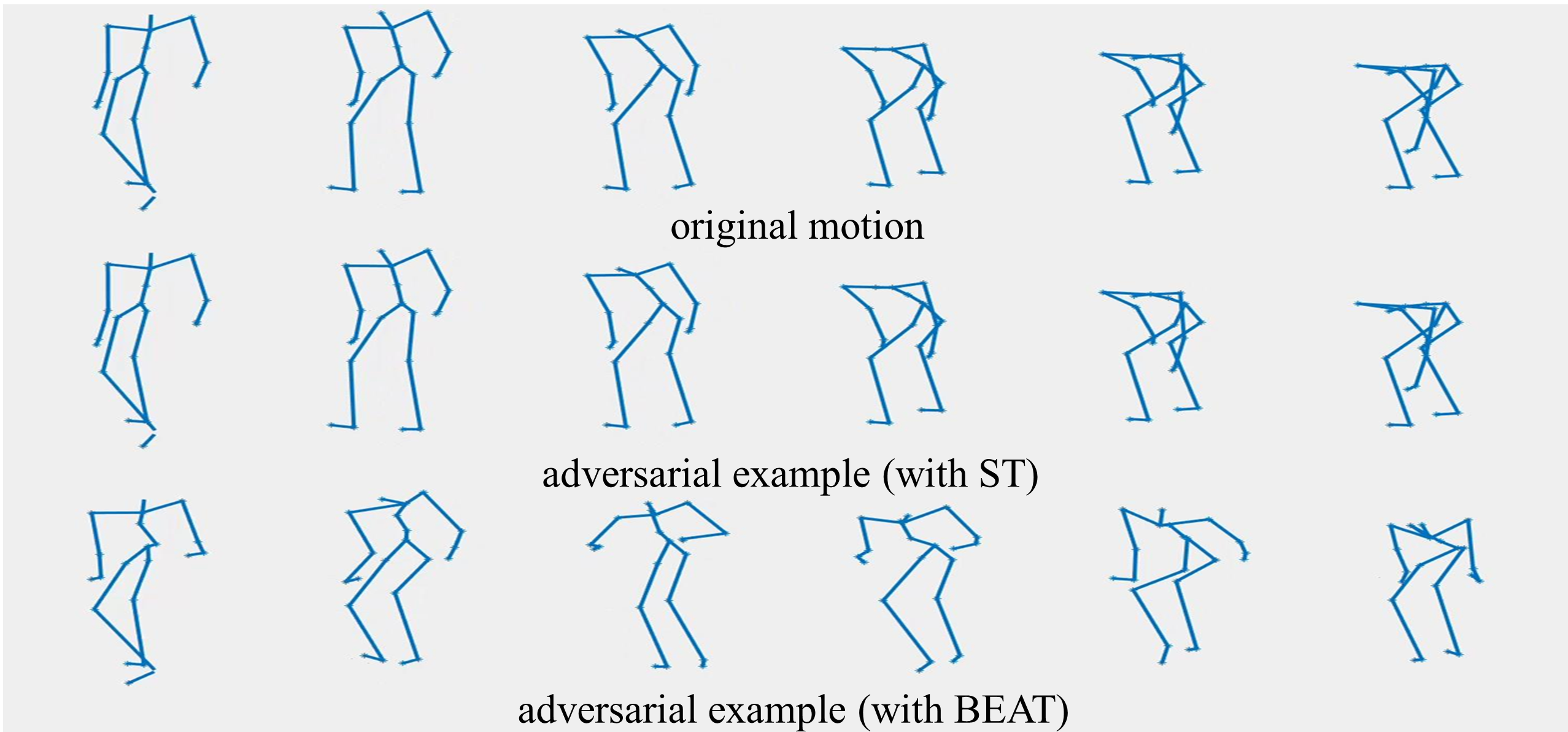
Figure 1: The original motion ‘deposit’ (top) is attacked by BASAR on standard trained model (middle) and BEAT trained model (bottom) separately. The visual difference of the original motion and the attacked motion on BEAT is bigger, compared with the attacked motion on ST.

	STGCN	CTRGCN	SGN	MSG3D
$l$ $\uparrow$	0.77/0.82	0.67/0.79	0.84/1.05	0.20/0.28
$\Delta a$ $\uparrow$	0.21/0.22	0.14/0.14	0.05/0.07	0.086/0.095
$\Delta B/B$ $\uparrow$	0.42%/0.77%	0.80%/0.94%	1.1%/1.5%	1.1%/1.2%
$l$ $\uparrow$	0.03/0.05	0.05/0.06	0.06/0.08	0.09/0.09
$\Delta a$ $\uparrow$	0.015/0.017	0.02/0.03	0.003/0.004	0.03/0.04
$\Delta B/B$ $\uparrow$	4.2%/4.8%	6.5%/7.4%	1.3%/1.7%	8.9%/11.0%
$l$ $\uparrow$	0.03/0.04	0.04/0.06	0.087/0.103	0.06/0.08
$\Delta a$ $\uparrow$	0.015/0.018	0.019/0.022	0.005/0.006	0.02/0.03
$\Delta B/B$ $\uparrow$	4.0%/4.7%	5.4%/5.6%	2.3%/2.7%	6.8%/9.0%

Table 2: Untargeted attack on HDM05 (top), NTU60 (middle) and NTU120 (bottom) from BASAR. xxx/xxx is pre/post BEAT results.

4.3 Additional Performance Analysis

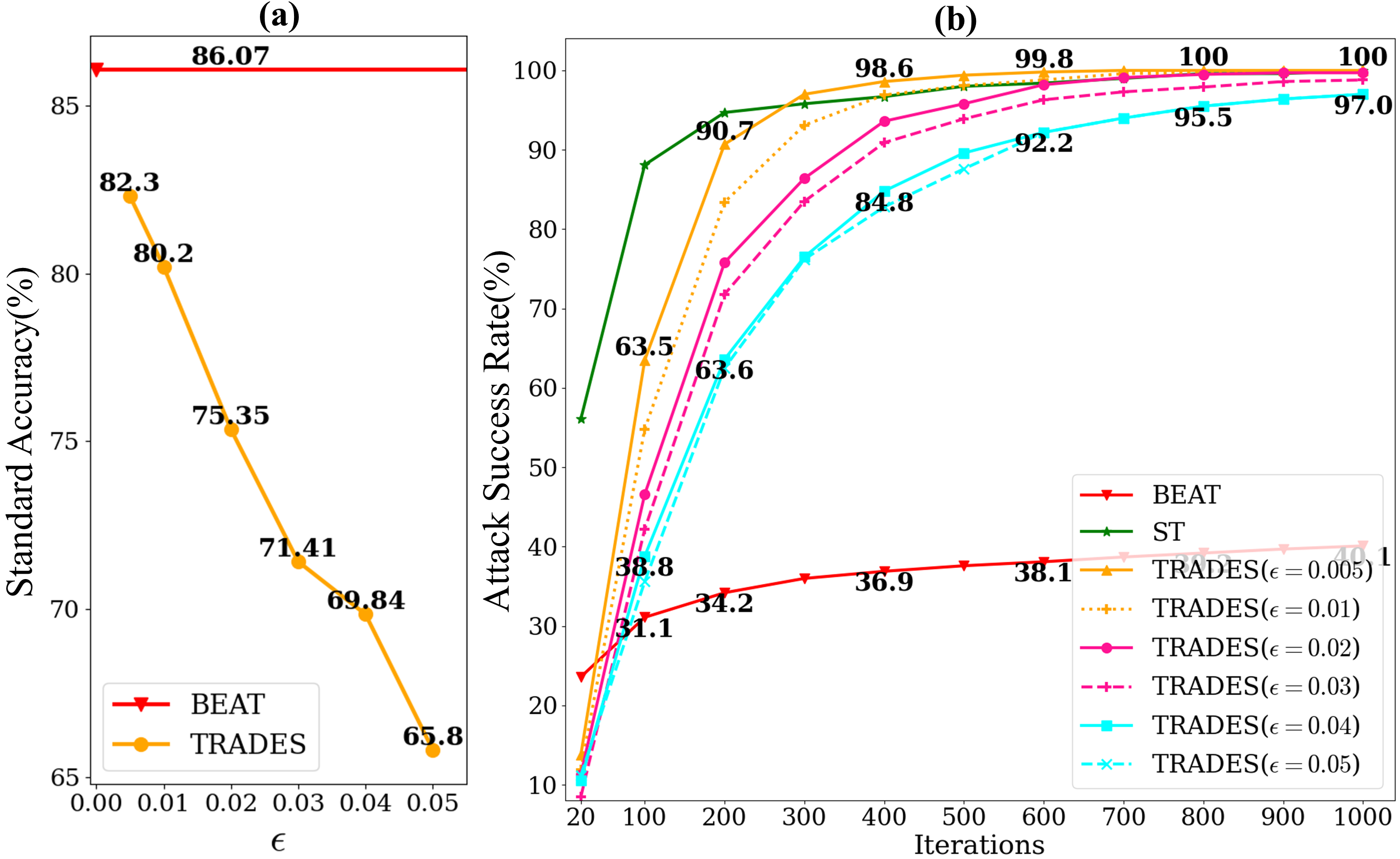
Figure 2: Comparisons with TRADES with different perturbation budget ($\epsilon$) on NTU60 with SGN. (a): standard accuracy vs. $\epsilon$; (b): results against SMART with 20 to 1000 iterations.

Comparison with other AT methods.

As shown in  Tab. 1, all baseline methods perform worse than BEAT, sometimes completely fail, e.g. failing to defend against SMART-1000 in large-scale datasets (NTU 60 and NTU 120). After investigating their defenses against SMART from iteration 20 to 1000 (Appendix A), we found the key reason is the baseline methods overly rely on the aggressiveness of the adversaries sampled during training. To verify it, we increase the perturbation budget $\epsilon$ from 0.005 to 0.05 during training in TRADES, and plot their standard accuracy & attack success rate (ASR) vs. $\epsilon$ in Fig. 2. Note that BEAT does not rely on a specific attacker. We find TRADES is highly sensitive to $\epsilon$ values: larger perturbations in adversarial training improve the defense (albeit still less effective than BEAT), but harm the standard accuracy (Fig. 2(a)). Further, sampling adversaries with more iterations (e.g. 1000 iterations) during AT may also improve the robustness (still worse than BEAT Fig. 2(b)) but is prohibitively slow, while BEAT requires much smaller computational overhead (see Sec. 4.1).

Does BEAT Obfuscate Gradients?

Since BEAT averages the gradient across different models, we investigate whether its robustness is due to obfuscated gradients, because obfuscated gradients can be circumvented and are not truly robust (Athalye, Carlini, and Wagner 2018). One way to verify this is to test BEAT on black-box attacks (Athalye, Carlini, and Wagner 2018), which we have demonstrated in Sec. 4.2. To be certain, we design another attack which can also circumvent defense relying on obfuscated gradients. We deploy an adaptive attack called EoT-SMART based on (Tramer et al. 2020): in each step, we estimate the expected gradient by averaging the gradients of multiple randomly interpolated samples. Tab. 3 shows that EoT-SMART performs only slightly better than SMART, demonstrating that BEAT does not rely on obfuscated gradients.

BEAT	ST-GCN	CTR-GCN	SGN	MS-G3D
HDM05	62.29% (+0.8%)	68.40% (+3.5%)	27.31% (+0.5%)	21.43% (+1.2%)
NTU 60	63.23% (+0.2%)	73.03% (-0.1%)	41.99% (+1.9%)	32.30% (-0.0%)

Table 3: Attack success rate (ASR) of EOT-SMART. ($\pm$xx%) means the ASR difference with SMART.

4.4 Ablation Study

Number of Appended Models

Although BNNs theoretically require sampling of many models for inference, in practice, we find a small number of models suffice. To show this, we conduct an ablation study on the number of appended models (N in Sec. 3.3). As shown in Tab. 4, with $N$ increasing, BEAT significantly lowers the attack success rates, which shows the Bayesian treatment of the model parameters is able to greatly increase the robustness. Further, when N $>$ 5, there is a diminishing gain with a slight improvement in robustness but also with increased computation. So we use N=5 by default.

We further show why our post-train Bayesian strategy is able to greatly increase the robustness. The classification loss gradient with respect to data is key to many attack methods. In a deterministic model, this gradient is computed on one model; in BEAT, this gradient is averaged over all models, i.e. the expected loss gradient. Theoretically, with an infinitely wide network in the large data limit, the expected loss gradient achieves 0, which is the source of the good robustness of BNNs (Bortolussi et al. 2022). To investigate whether BEAT’s robustness benefits from the vanishing expected gradient, we randomly sample 500 motions from the testing data and sample one frame from each motion. Then we compute their expected loss gradients and plot a total of 37500 loss gradient components in Fig. 3 (a), where each dot represents a component of the expected loss gradient of one frame. Fig. 3 (b) shows the percentage of the expected gradient components close to 0. Figure 3 essentially shows the empirical distribution of the component-wise expected loss gradient. When $N$ increases, the gradient components steadily approach zero, indicating a vanishing expected loss gradient which provides robustness (Bortolussi et al. 2022).

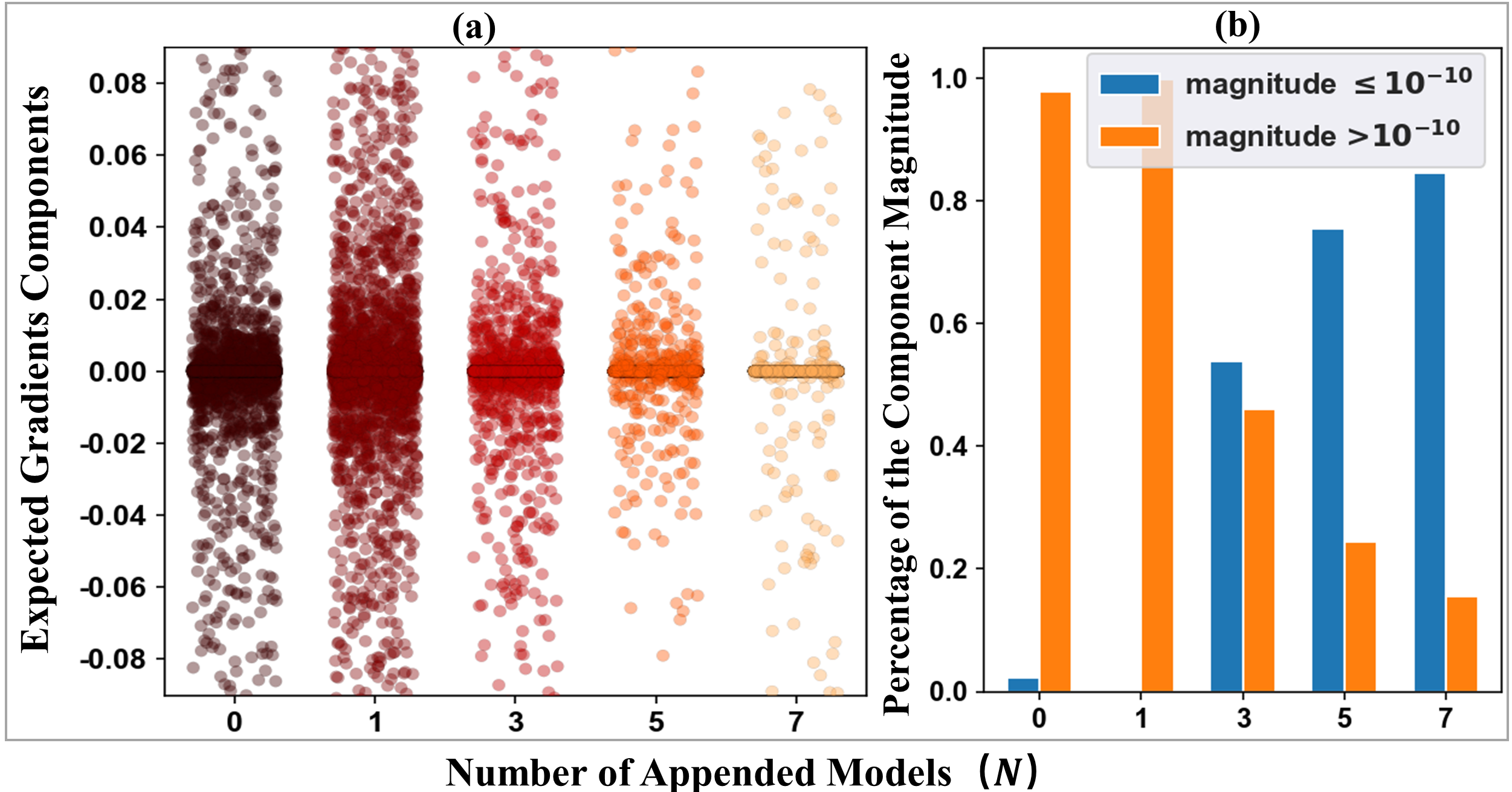
Figure 3: The components of the expected loss gradients of BEAT on NTU60 with SGN. $N=0$ is standard training. (a): the empirical distribution of gradient components; (b): the percentage of the expected gradient components with magnitude above and below 10^-10.

Joint Distribution of Data and Adversaries

Other than the Bayesian treatment of models, BEAT also benefits from the Bayesian treatment on the adversaries. To see its contribution, we plug-and-play our post-train Bayesian strategy to other AT methods which do not model the adversarial distribution. Specifically, we design a post-train Bayesian TRADES (PB+TRADES) with different number of appended models, and compare them with BEAT in Tab. 4. While both BEAT and PB+TRADES benefit from BNNs, BEAT still outperforms PB+TRADES by large margins. Note the major difference between BEAT and PB+TRADES is whether to consider the full adversarial distribution, which shows the benefit of bringing the full adversarial distribution into the joint probability.

N	Standard Accuracy$\uparrow$		Attack Success Rate$\downarrow$
	BEAT	PB+TRADES	BEAT	PB+TRADES
1	84.90	83.66%	96.39%	97.40%
3	85.72%	84.96%	57.13%	80.37%
5	86.07%	84.74%	40.10%	59.03%
7	86.01%	84.86%	27.40%	48.97%

Table 4: Ablation Study on NTU 60 with SGN as the base classifier. ‘N’is the number of appended models. ‘PB’ means Post-train Bayesian strategy. ‘Attack Success Rate’ is the defense results against SMART-1000.

5 Discussion, Conclusions and Future Work

One limitation is prior knowledge is needed on $d(\mathbf{x},\tilde{\mathbf{x}})$ in Eq. 4, either explicitly as BEAT or implicitly e.g. using another model to learn the data manifold. However, this is lightweight as manifold learning/representation is a rather active field and many methods could be used. BEAT can potentially incorporate any manifold representation. Also, we assume that all adversarial samples are distributed closely to the data manifold, which is true for images (Stutz, Hein, and Schiele 2019) and skeletal motion (Diao et al. 2021), but not necessarily for other data.

To our best knowledge, we proposed the first black-box defense for skeleton-based HAR. Our method BEAT is underpinned by a new Bayesian Energy-based Adversarial Training framework, and is evaluated across various classifiers, datasets and attackers. Our method employs a post-train strategy for fast training and a full Bayesian treatment on normal data, the adversarial samples and the classifier, without adding much extra computational cost. In future, we will extend BEAT to more data types, both time-series and static, such as videos and stock prices, as well as implicit manifold parameterization for images, by employing task/data specific $d(\mathbf{x},\tilde{\mathbf{x}})$ in Eq. 5.

6 Acknowledgment

This project has received funding from the European Union’s Horizon 2020 research and innovation programme under grant agreement No 899739 CrowdDNA.

References

- Akhtar et al. (2021) Akhtar, N.; Mian, A.; Kardan, N.; and Shah, M. 2021. Advances in adversarial attacks and defenses in computer vision: A survey. arXiv:2108.00401 [cs]. ArXiv: 2108.00401.
- Athalye, Carlini, and Wagner (2018) Athalye, A.; Carlini, N.; and Wagner, D. 2018. Obfuscated gradients give a false sense of security: Circumventing defenses to adversarial examples. In International conference on machine learning, 274–283. PMLR.
- Athalye et al. (2018) Athalye, A.; Engstrom, L.; Ilyas, A.; and Kwok, K. 2018. Synthesizing robust adversarial examples. In International conference on machine learning, 284–293. PMLR.
- Bai et al. (2021) Bai, T.; Luo, J.; Zhao, J.; Wen, B.; and Wang, Q. 2021. Recent Advances in Adversarial Training for Adversarial Robustness. In Proceedings of the Thirtieth International Joint Conference on Artificial Intelligence, IJCAI, 4312–4321.
- Bortolussi et al. (2022) Bortolussi, L.; Carbone, G.; Laurenti, L.; Patane, A.; Sanguinetti, G.; and Wicker, M. 2022. On the Robustness of Bayesian Neural Networks to Adversarial Attacks.
- Brendel, Rauber, and Bethge (2018) Brendel, W.; Rauber, J.; and Bethge, M. 2018. Decision-Based Adversarial Attacks: Reliable Attacks Against Black-Box Machine Learning Models. In 6th International Conference on Learning Representations, ICLR.
- Carlini and Wagner (2017) Carlini, N.; and Wagner, D. 2017. Towards evaluating the robustness of neural networks. In 2017 ieee symposium on security and privacy (sp), 39–57. IEEE.
- Carmon et al. (2019) Carmon, Y.; Raghunathan, A.; Schmidt, L.; Liang, P.; and Duchi, J. C. 2019. Unlabeled data improves adversarial robustness. In Proceedings of the 33rd International Conference on Neural Information Processing Systems, 11192–11203.
- Chakraborty et al. (2018) Chakraborty, A.; Alam, M.; Dey, V.; Chattopadhyay, A.; and Mukhopadhyay, D. 2018. Adversarial Attacks and Defences: A Survey. arXiv:1810.00069 [cs, stat]. ArXiv: 1810.00069.
- Chen et al. (2021) Chen, Y.; Zhang, Z.; Yuan, C.; Li, B.; Deng, Y.; and Hu, W. 2021. Channel-wise Topology Refinement Graph Convolution for Skeleton-Based Action Recognition. In Proceedings of the IEEE/CVF International Conference on Computer Vision, 13359–13368.
- Cohen, Rosenfeld, and Kolter (2019) Cohen, J. M.; Rosenfeld, E.; and Kolter, J. Z. 2019. Certified Adversarial Robustness via Randomized Smoothing. In ICML, volume 97 of Proceedings of Machine Learning Research, 1310–1320. PMLR.
- Dai et al. (2018) Dai, H.; Li, H.; Tian, T.; Huang, X.; Wang, L.; Zhu, J.; and Song, L. 2018. Adversarial attack on graph structured data. In International conference on machine learning, 1115–1124. PMLR.
- Diao et al. (2021) Diao, Y.; Shao, T.; Yang, Y.; Zhou, K.; and Wang, H. 2021. BASAR: Black-Box Attack on Skeletal Action Recognition. In IEEE Conference on Computer Vision and Pattern Recognition, CVPR, 2021, 7597–7607. Computer Vision Foundation / IEEE.
- Diao et al. (2022) Diao, Y.; Wang, H.; Shao, T.; Yang, Y.-L.; Zhou, K.; and Hogg, D. 2022. Understanding the Vulnerability of Skeleton-based Human Activity Recognition via Black-box Attack. arXiv:2211.11312 [cs]. ArXiv: 2211.11312.
- Dong et al. (2020) Dong, Y.; Deng, Z.; Pang, T.; Zhu, J.; and Su, H. 2020. Adversarial Distributional Training for Robust Deep Learning. Advances in Neural Information Processing Systems, 33: 8270–8283.
- Evtimov et al. (2017) Evtimov, I.; Eykholt, K.; Fernandes, E.; Kohno, T.; Li, B.; Prakash, A.; Rahmati, A.; and Song, D. 2017. Robust physical-world attacks on machine learning models. arXiv preprint arXiv:1707.08945, 2(3): 4.
- Goodfellow, Shlens, and Szegedy (2015) Goodfellow, I. J.; Shlens, J.; and Szegedy, C. 2015. Explaining and Harnessing Adversarial Examples. In Bengio, Y.; and LeCun, Y., eds., 3rd International Conference on Learning Representations, ICLR 2015, San Diego, CA, USA, May 7-9, 2015, Conference Track Proceedings.
- Grathwohl et al. (2020) Grathwohl, W.; Wang, K.-C.; Jacobsen, J.-H.; Duvenaud, D.; Norouzi, M.; and Swersky, K. 2020. Your classifier is secretly an energy based model and you should treat it like one. In International Conference on Learning Representations.
- Hill, Mitchell, and Zhu (2021) Hill, M.; Mitchell, J. C.; and Zhu, S. 2021. Stochastic Security: Adversarial Defense Using Long-Run Dynamics of Energy-Based Models. In 9th International Conference on Learning Representations, ICLR 2021.
- Hwang et al. (2021) Hwang, J.; Kim, J.-H.; Choi, J.-H.; and Lee, J.-S. 2021. Just One Moment: Structural Vulnerability of Deep Action Recognition Against One Frame Attack. In Proceedings of the IEEE/CVF International Conference on Computer Vision, 7668–7676.
- Karim, Majumdar, and Darabi (2020) Karim, F.; Majumdar, S.; and Darabi, H. 2020. Adversarial attacks on time series. IEEE Transactions on Pattern Analysis and Machine Intelligence. Publisher: IEEE.
- Kumar et al. (2020) Kumar, D.; Kumar, C.; Seah, C. W.; Xia, S.; and Shao, M. 2020. Finding Achilles’ Heel: Adversarial Attack on Multi-modal Action Recognition. In Proceedings of the 28th ACM International Conference on Multimedia, 3829–3837.
- Lécuyer et al. (2019) Lécuyer, M.; Atlidakis, V.; Geambasu, R.; Hsu, D.; and Jana, S. 2019. Certified Robustness to Adversarial Examples with Differential Privacy. In 2019 IEEE Symposium on Security and Privacy, SP 2019, 656–672. IEEE.
- Lee, Yang, and Oh (2020) Lee, K.; Yang, H.; and Oh, S.-Y. 2020. Adversarial Training on Joint Energy Based Model for Robust Classification and Out-of-Distribution Detection. 2020 20th International Conference on Control, Automation and Systems (ICCAS), 17–21.
- Liang et al. (2018) Liang, B.; Li, H.; Su, M.; Bian, P.; Li, X.; and Shi, W. 2018. Deep text classification can be fooled. In Proceedings of the 27th International Joint Conference on Artificial Intelligence, 4208–4215.
- Liu et al. (2020a) Liu, C.; Salzmann, M.; Lin, T.; Tomioka, R.; and Süsstrunk, S. 2020a. On the Loss Landscape of Adversarial Training: Identifying Challenges and How to Overcome Them. In Advances in Neural Information Processing Systems, volume 33, 21476–21487.
- Liu, Akhtar, and Mian (2020) Liu, J.; Akhtar, N.; and Mian, A. 2020. Adversarial Attack on Skeleton-Based Human Action Recognition. IEEE transactions on neural networks and learning systems, PP.
- Liu et al. (2020b) Liu, J.; Shahroudy, A.; Perez, M.; Wang, G.; Duan, L.-Y.; and Kot, A. C. 2020b. NTU RGB+D 120: A large-scale benchmark for 3D human activity understanding. IEEE Transactions on Pattern Analysis and Machine Intelligence, 42(10): 2684–2701.
- Liu et al. (2020c) Liu, Z.; Zhang, H.; Chen, Z.; Wang, Z.; and Ouyang, W. 2020c. Disentangling and Unifying Graph Convolutions for Skeleton-Based Action Recognition. In Proceedings of the IEEE/CVF Conference on Computer Vision and Pattern Recognition, 143–152.
- Madry et al. (2018) Madry, A.; Makelov, A.; Schmidt, L.; Tsipras, D.; and Vladu, A. 2018. Towards Deep Learning Models Resistant to Adversarial Attacks. In International Conference on Learning Representations.
- Miyato et al. (2018) Miyato, T.; Maeda, S.-i.; Koyama, M.; and Ishii, S. 2018. Virtual adversarial training: a regularization method for supervised and semi-supervised learning. IEEE transactions on pattern analysis and machine intelligence, 41(8): 1979–1993.
- Müller et al. (2007) Müller, M.; Röder, T.; Clausen, M.; Eberhardt, B.; Krüger, B.; and Weber, A. 2007. Documentation Mocap Database HDM05. Technical Report CG-2007-2, Universität Bonn. ISSN: 1610-8892.
- Pony, Naeh, and Mannor (2021) Pony, R.; Naeh, I.; and Mannor, S. 2021. Over-the-Air Adversarial Flickering Attacks against Video Recognition Networks. In Proceedings of the IEEE/CVF Conference on Computer Vision and Pattern Recognition, 515–524.
- Poursaeed et al. (2021) Poursaeed, O.; Jiang, T.; Yang, H.; Belongie, S.; and Lim, S.-N. 2021. Robustness and Generalization via Generative Adversarial Training. In Proceedings of the IEEE/CVF International Conference on Computer Vision, 15711–15720.
- Raghunathan et al. (2020) Raghunathan, A.; Xie, S. M.; Yang, F.; Duchi, J.; and Liang, P. 2020. Understanding and Mitigating the Tradeoff between Robustness and Accuracy. In International Conference on Machine Learning, 7909–7919. PMLR.
- Saatci and Wilson (2017) Saatci, Y.; and Wilson, A. G. 2017. Bayesian GAN. In Advances in Neural Information Processing Systems, volume 30. Curran Associates, Inc.
- Shahroudy et al. (2016) Shahroudy, A.; Liu, J.; Ng, T.-T.; and Wang, G. 2016. NTU RGB+D: A large scale dataset for 3D human activity analysis. In Proceedings of the IEEE conference on computer vision and pattern recognition, 1010–1019.
- Silva and Najafirad (2020) Silva, S. H.; and Najafirad, P. 2020. Opportunities and Challenges in Deep Learning Adversarial Robustness: A Survey. arXiv:2007.00753 [cs, stat]. ArXiv: 2007.00753.
- Song et al. (2020) Song, C.; He, K.; Lin, J.; Wang, L.; and Hopcroft, J. E. 2020. Robust Local Features for Improving the Generalization of Adversarial Training. In 8th International Conference on Learning Representations, ICLR. OpenReview.net.
- Song et al. (2018) Song, C.; He, K.; Wang, L.; and Hopcroft, J. E. 2018. Improving the Generalization of Adversarial Training with Domain Adaptation. In International Conference on Learning Representations.
- Stutz, Hein, and Schiele (2019) Stutz, D.; Hein, M.; and Schiele, B. 2019. Disentangling adversarial robustness and generalization. In CVPR, 6976–6987.
- Stutz, Hein, and Schiele (2020) Stutz, D.; Hein, M.; and Schiele, B. 2020. Confidence-calibrated adversarial training: Generalizing to unseen attacks. In International Conference on Machine Learning, 9155–9166. PMLR.
- Tanaka, Kera, and Kawamoto (2021) Tanaka, N.; Kera, H.; and Kawamoto, K. 2021. Adversarial Bone Length Attack on Action Recognition. arXiv preprint arXiv:2109.05830.
- Tang et al. (2022) Tang, X.; Wang, H.; Hu, B.; Gong, X.; Yi, R.; Kou, Q.; and Jin, X. 2022. Real-Time Controllable Motion Transition for Characters. ACM Trans. Graph., 41(4).
- Tramer et al. (2020) Tramer, F.; Carlini, N.; Brendel, W.; and Madry, A. 2020. On adaptive attacks to adversarial example defenses. Advances in Neural Information Processing Systems, 33: 1633–1645.
- Tsipras et al. (2019) Tsipras, D.; Santurkar, S.; Engstrom, L.; Turner, A.; and Madry, A. 2019. Robustness May Be at Odds with Accuracy. In International Conference on Learning Representations.
- Uesato et al. (2018) Uesato, J.; O’donoghue, B.; Kohli, P.; and Oord, A. 2018. Adversarial risk and the dangers of evaluating against weak attacks. In International Conference on Machine Learning, 5025–5034. PMLR.
- Wang et al. (2021a) Wang, H.; He, F.; Peng, Z.; Shao, T.; Yang, Y.; Zhou, K.; and Hogg, D. 2021a. Understanding the Robustness of Skeleton-based Action Recognition under Adversarial Attack. In Proceedings of the IEEE/CVF Conference on Computer Vision and Pattern Recognition (CVPR).
- Wang, Ho, and Komura (2015) Wang, H.; Ho, E. S.; and Komura, T. 2015. An energy-driven motion planning method for two distant postures. IEEE transactions on visualization and computer graphics, 21(1): 18–30. Publisher: IEEE.
- Wang et al. (2021b) Wang, H.; Ho, E. S. L.; Shum, H. P. H.; and Zhu, Z. 2021b. Spatio-Temporal Manifold Learning for Human Motions via Long-Horizon Modeling. IEEE Transactions on Visualization and Computer Graphics, 27(1): 216–227.
- Wang et al. (2013) Wang, H.; Sidorov, K. A.; Sandilands, P.; and Komura, T. 2013. Harmonic parameterization by electrostatics. ACM Transactions on Graphics (TOG), 32(5): 155.
- Wang et al. (2020) Wang, Y.; Zou, D.; Yi, J.; Bailey, J.; Ma, X.; and Gu, Q. 2020. Improving Adversarial Robustness Requires Revisiting Misclassified Examples. In 8th International Conference on Learning Representations, ICLR 2020. OpenReview.net.
- Wei et al. (2019) Wei, X.; Zhu, J.; Yuan, S.; and Su, H. 2019. Sparse adversarial perturbations for videos. In Proceedings of the AAAI Conference on Artificial Intelligence.
- Wei et al. (2020) Wei, Z.; Chen, J.; Wei, X.; Jiang, L.; Chua, T.; Zhou, F.; and Jiang, Y. 2020. Heuristic Black-Box Adversarial Attacks on Video Recognition Models. In The Thirty-Fourth AAAI Conference on Artificial Intelligence, 12338–12345.
- Yan, Xiong, and Lin (2018) Yan, S.; Xiong, Y.; and Lin, D. 2018. Spatial temporal graph convolutional networks for skeleton-based action recognition. In Thirty-second AAAI conference on artificial intelligence.
- Yang et al. (2020) Yang, Y.; Rashtchian, C.; Zhang, H.; Salakhutdinov, R. R.; and Chaudhuri, K. 2020. A Closer Look at Accuracy vs. Robustness. In Advances in Neural Information Processing Systems.
- Ye and Zhu (2018) Ye, N.; and Zhu, Z. 2018. Bayesian Adversarial Learning. In Advances in Neural Information Processing Systems, volume 31. Curran Associates, Inc.
- Zhang et al. (2019a) Zhang, H.; Yu, Y.; Jiao, J.; Xing, E.; El Ghaoui, L.; and Jordan, M. 2019a. Theoretically principled trade-off between robustness and accuracy. In International Conference on Machine Learning, 7472–7482. PMLR.
- Zhang et al. (2019b) Zhang, H.; Yu, Y.; Jiao, J.; Xing, E. P.; Ghaoui, L. E.; and Jordan, M. I. 2019b. Theoretically Principled Trade-off between Robustness and Accuracy. In Proceedings of the 36th International Conference on Machine Learning, ICML, volume 97 of Proceedings of Machine Learning Research, 7472–7482. PMLR.
- Zhang et al. (2020a) Zhang, H.; Zhu, L.; Zhu, Y.; and Yang, Y. 2020a. Motion-Excited Sampler: Video Adversarial Attack with Sparked Prior. In Computer Vision–ECCV 2020: 16th European Conference, Glasgow, UK, August 23–28, 2020, Proceedings, Part XX 16, 240–256. Springer.
- Zhang et al. (2020b) Zhang, P.; Lan, C.; Zeng, W.; Xing, J.; Xue, J.; and Zheng, N. 2020b. Semantics-Guided Neural Networks for Efficient Skeleton-Based Human Action Recognition. In Proceedings of the IEEE Conference on Computer Vision and Pattern Recognition.
- Zheng et al. (2020) Zheng, T.; Liu, S.; Chen, C.; Yuan, J.; Li, B.; and Ren, K. 2020. Towards understanding the adversarial vulnerability of skeleton-based action recognition. arXiv preprint arXiv:2005.07151.
- Zhu et al. (2021) Zhu, Y.; Ma, J.; Sun, J.; Chen, Z.; Jiang, R.; Chen, Y.; and Li, Z. 2021. Towards understanding the generative capability of adversarially robust classifiers. In Proceedings of the IEEE/CVF International Conference on Computer Vision, 7728–7737.
- Zügner, Akbarnejad, and Günnemann (2018) Zügner, D.; Akbarnejad, A.; and Günnemann, S. 2018. Adversarial attacks on neural networks for graph data. In Proceedings of the 24th ACM SIGKDD International Conference on Knowledge Discovery & Data Mining, 2847–2856.