Small Errors Imply Large Instabilities

Abstract

Numerical Analysts and scientists working in applications often observe that once they improve their techniques to get a better accuracy, some instability creeps in through the back door. This paper shows for a large class of numerical methods that such a Trade-off Principle between error and stability is unavoidable. It is an instance of a no free lunch theorem. The setting is confined to recovery of functions from data, but it includes solving differential equations by writing such methods as a recovery of functions under constraints imposed by differential operators and boundary values. It is shown in particular that Kansa’s Unsymmetric Collocation Method sacrifices accuracy for stability, when compared to symmetric collocation.

MSC Classification]41Axx, 65D05, 65D12, 65D15

1 Introduction

After quite some efforts to find kernels that allow small recovery errors and well-conditioned kernel matrices at the same time, the paper schaback:1995-1 proved that this does not work. The result was called “Uncertainty Relation” or “Trade-off Principle” (see e.g. Holger Wendland’s book wendland:2005-1 of 2005) and received quite some attention in the literature. It is a special case of the “No free lunch” principle. As correctly mentioned by Greg Fasshauer and Michael McCourt in their 2015 book fasshauer-mccourt:2015-1 , it had quite some negative influence on the development of the field, because it kept users from looking at better bases than those spanned by kernel translates. But it will turn out here that changes of bases will not really help as long as the other ingredients are fixed.

Sparked by a question of C.S. Chen of the University of Southern Mississippi in an e-mail dated Dec. 28th, 2021, this paper extends the result of schaback:1995-1 to much more general situations. To avoid the misconceptions implied by schaback:1995-1 , the effect of basis changes will be discussed at various places. But most of the results here are independent of choices of bases.

Since the scope of the paper will be quite wide, a good deal of abstraction will be necessary later, and therefore a classical case should be served as starters. Consider interpolation of functions $f\in C^{n+1}[-1,+1]$ on a set $X_{n}$ of points $-1\leq x_{0}<x_{1},\ldots<x_{n}\leq 1$ by polynomials $I_{n}(f)$ of degree at most $n$. The well-known error bound is

$$\lvert f(x)-I_{n}(f)(x)\rvert\leq\dfrac{\|f^{(n+1)}\|_{\infty}}{(n+1)!}\prod_{j=0}^{n}\lvert x-x_{j}\rvert$$

based on Newton’s formula. We can recast this as an error bound

$$\lvert f(x)-I_{n}(f)(x)\rvert\leq P_{X_{n}}(x)\|f^{(n+1)}\|_{\infty}$$

in terms of a Power Function

$$\begin{array}[]{rcl}P_{X_{n}}(x)&:=&\displaystyle{\sup_{\|f^{(n+1)}\|_{\infty}\leq 1}\lvert f(x)-I_{n}(f)(x)\rvert}\\ &=&\displaystyle{\frac{1}{(n+1)!}\prod_{j=0}^{n}\lvert x-x_{j}\rvert}.\end{array}$$

If we add a point $x$ to the set $X_{n}$, the Lagrangian of degree $n+1$, vanishing on $X_{n}$ and being one on $x$ is

$$u_{x,X_{n}}(z)=\prod_{j=0}^{n}\frac{z-x_{j}}{x-x_{j}}$$

with seminorm

$$\|u^{(n+1)}_{x,X_{n}}\|_{\infty}=(n+1)!\prod_{j=0}^{n}\lvert x-x_{j}\rvert^{-1},$$

leading to

$$1=P_{X_{n}}(x)\cdot\|u^{(n+1)}_{x,X_{n}}\|_{\infty}.$$ (1)

This is a Trade-off Principle:

Small Power Functions lead to large norms of Lagrangians.

Since Lagrangians are the images of unit data in the function space, large norms of Lagrangians lead to large norms of interpolation operators as maps from data to functions. Then small data variations lead to large variations in the resulting functions, and one may call this a grade of evaluation instability. Thus the Trade-off Principle implies

Small errors lead to large evaluation instabilities.

The paper gives a rigid underpinning to this somewhat sloppy statement. Recall that regularization of operator equations works exactly in the same way: part of the recovery error is sacrificed for better stability.

However, the numerical computation of the Lagrangians induces additional instabilities that are ignored here. To cope with these, barycentric formulas were introduced for the polynomial case, see J.P. Berrut and L.N. Trefethen berrut-trefethen:2004-1 . For kernel-based recoveries, various methods were invented to cope with instabilities, see the references given in Section 11.

Section 2 sets the stage for general recovery methods including solving differential equations. Recovery processes reconstruct functions from data given as prescribed values of linear functionals, and the evaluation of the result will again be an application of a functional. Data can include values of arbitrary linear operators acting on functions, thus rewriting methods for PDE solving as function recoveries.

Section 3 introduces the form of the recoveries considered. Nearest-neighbor methods, optimal recoveries in Hilbert spaces, and regression in Machine Learning are special cases described in Section 4.

The basic technique used for trade-off principles is outlined in Section 5, still in rather abstract form. Then Section 6 contains the central results, namely trade-off principles that bound the product of norms of errors and norms of certain worst-case functions from below. It is shown how the latter govern instability of the evaluation of the recovery. The lower bounds turn into equalities in case of optimal recoveries in Section 7.

Examples are given in Section 8, including splines and recoveries via expansions like Fourier or Taylor series. The connection to the older trade-off principle from schaback:1995-1 is provided in Section 8.7, followed by extensions to unsymmetric methods like Kansa’s collocation technique. The trade-off principle holds for these as well, but they sacrifice accuracy for evaluation stability. Finally, the implications for greedy adaptive methods are sketched.

2 Data as Functionals

A fairly general and useful viewpoint on Numerical Analysis or Computational Mathematics when working on functions is to see data of a function as values of linear functionals. In particular, differential equations, ordinary or partial, just impose infinitely many restrictions on a function $u$ from some function space $U$ by applying linear functionals. This can be conveniently written as

$$\lambda(u)=f_{\lambda}\in\mathbb{R}$$ (2)

for all functionals $\lambda$ from a subset $\Lambda$ of the dual $U^{*}$ of $U$, the space of continuous linear functionals on $U$. The problem is to recover $u$ from the given data $f_{\lambda}$. The specifics of certain differential equation problems involving differential or boundary evaluation operators disappear. And if users have only limited information in the sense of just finitely many data $f_{\lambda_{j}}\in\mathbb{R}$ for a finite subset $\Lambda_{M}=\{\lambda_{1},\ldots,\lambda_{M}\}\subset\Lambda$, one has to use computational techniques that get along with the available data. This viewpoint is behind the scenes for this paper. Readers should always be aware that differential operators may lurk behind the functionals appearing here.

For illustration, consider a standard Poisson problem

$$\begin{array}[]{rcll}\Delta u&=&f&\hbox{ in }\Omega\\ u&=&g&\hbox{ in }\partial\Omega\\ \end{array}$$ (3)

on a bounded domain $\Omega\subset\mathbb{R}^{2}$ for simplicity. The data functionals come in two variations:

$$\begin{array}[]{rclll}\Delta_{i}(f)&:=&\Delta f(x_{i}),&x_{i}\in\overline{\Omega},&1\leq i\leq M_{\Delta}\\ \beta_{j}(f)&=&f(y_{j}),&y_{j}\in\partial\Omega,&1\leq j\leq M_{\beta}\\ \end{array}$$ (4)

caring for the PDE in the domain and for the boundary values. They are finite selections from the obvious infinite sets of functionals that define the true solution analytically. If the analytic problem is well-posed and if the function recovery from the above data is carried out with enough oversampling, this technique produces accurate and convergent approximations to the true solution of the PDE problem schaback:2016-4 . This reference also fits algorithms that solve problems in weak form into this framework, including the Meshless Local Petrov Galerkin approach by S.N. Atluri and T.-L. Zhu atluri-zhu:1998-2 ; atluri-zhu:1998-1 and Generalized Finite Element Methods, see the survey by I. Babuška et.al. babuska-et-al:2003-1 . The general practical observation is that going for more accuracy causes more instabilities, in a way that will be clarified here.

Also, evaluation of functions is the application of a functional $\mu\in U^{*}$ to some function $f$. In particular, evaluation of a multivariate derivative $D^{\alpha}$ at a point $x$ is the application of the functional $\delta_{x}(D^{\alpha}f)=f^{(\alpha)}(x)$ in case that $\delta_{x}D^{\alpha}$ is continuous on $U$. If point evaluation is not defined, as in $L_{2}$ spaces, but if local integration is feasible, one can evaluate local integral means, as substitutes for point evaluation. This is the standard way to handle problems in weak form in the references cited above.

Summarizing, everything boils down to a matter of functionals. What can we say about $\mu(f)$ if we know all $\lambda(f)$ for all $\lambda\in\Lambda$? In particular, what can we say about $f(x)$ when we know plenty of data $f(x_{j})$? Note that this problem is regression in a probabilistic context, and it arises in Machine Learning on a large scale, with Big Data given in high-dimensional spaces.

3 Recovery of Functions

We now postulate that we can write the recovery of functions $f$ from their data $\Lambda(f)=(\lambda_{1}(f),\ldots,\lambda_{M}(f))^{T}\in\mathbb{R}^{M}$ as a linear recovery map

$$f\mapsto R_{a_{\Lambda}}(f):=a^{T}_{\Lambda}\Lambda(f)=\displaystyle{\sum_{\lambda_{j}\in\Lambda}a_{\lambda_{j}}\lambda_{j}(f)}\hbox{ for all }f\in U$$ (5)

such that the span of the elements $a_{\lambda_{j}}$ of the vector $a_{\Lambda}\in U^{M}$ defines a trial subspace of functions in $U$. To avoid certain complications, the map $f\to\Lambda(f)\in\mathbb{R}^{M}$ is assumed to be surjective.

We call the recovery process interpolatory if the recovery preserves the data, i.e.

$$\Lambda(R_{a_{\Lambda}}(f))=\Lambda(a_{\Lambda}^{T}\Lambda(f))=\Lambda(f)\hbox{ for all }f\in U,$$

and then $\lambda_{k}(a_{\lambda_{j}})=\delta_{jk},\,1\leq j,k\leq M$ holds and the $a_{\lambda_{j}}$ form a Lagrange basis with Kronecker data. We shall use the notation $u_{\mu,\Lambda}$ for a Lagrangian that satisfies $\Lambda(u_{\mu,\Lambda})=0,\;\mu(u_{\mu,\Lambda})=1$, and then $a_{\lambda_{j}}=u_{\lambda_{j},\Lambda\setminus\{\lambda_{j}\}}$ holds in this notation.

Lagrangians will not exist for general recoveries. But the $a_{\lambda_{j}}$ may be called pseudo-Lagrangians because they produce the recovery like Lagrangians, but without exact reproduction of the data.

Evaluation of the recovery via a functional $\mu$ now is

$$\mu(a^{T}_{\Lambda}\Lambda(f))=a^{T}_{\Lambda}(\mu)\Lambda(f)=\displaystyle{\sum_{\lambda_{j}\in\Lambda}\mu(a_{\lambda_{j}})\lambda_{j}(f)}$$

by defining a vector $a^{T}_{\Lambda}(\mu):=\mu(a^{T}_{\Lambda})$ that is a bilinear form in $\Lambda$ and $\mu$.

One may restrict these maps to sums over neighbours $\lambda$ of $\mu$, to get more locality, and this is what generalized Moving Least Squares farwig:1986-1 ; levin:1998-1 ; wendland:2000-1 ; armentano:2001-1 or Finite Elements do. But if theoretically done for all $\mu\in U^{*}$, this still fits into the above framework. As a prominent example, Barycentric formulas by J.P. Berrut and L.N. Trefethen berrut-trefethen:2004-1 change the way the above formula is calculated, with a significant gain in numerical stability.

For recovery of a single value $\mu(f)$ from single values $\lambda_{j}(f)$ one can construct a vector of single values $a_{\lambda_{j}}(\mu)$ such that

$$\mu(f)\approx\displaystyle{\sum_{\lambda_{j}\in\Lambda}a_{\lambda_{j}}(\mu)\lambda_{j}(f)}$$ (6)

without necessarily calculating the $a_{\lambda_{j}}$ as functions and taking values $\mu(a_{\lambda_{j}})=a_{\lambda_{j}}(\mu)$ afterwards. In meshless methods (see the early survey by T. Belytschko et.al. belytschko-et-al:1996-1 ), the functions $a_{\lambda_{j}}$ are called shape functions. In the standard approach, they are calculated in many points, and if derivatives are needed for dealing with PDEs, these are taken afterwards or obtained by taking derivatives of the local construction process. In contrast to this, Direct Moving Least Squares by D. Mirzaei et.al. mirzaei-et-al:2012-1 , mirzaei-schaback:2013-1 use (6) for derivative functionals $\mu$ without the detour via shape functions.

This presentation looks unduly abstract, but it isn’t. It considers recovery without any fixed assumptions about how functions are represented, how norms of errors and functions are defined, and how bases are chosen. Therefore it allows to compare actual numerical strategies on a higher level. It goes back to the input data and considers the output data, as functionals, the actual determination of the recovery map being in a black box. The final goal in this paper is to see whether going for a small error implies some sort of instability whatsoever, and this may be independent of what happens in the black box. This is why we consider errors and stability in section 6 after we present some examples.

4 Special Recovery Strategies

When avoiding full functions, the recovery of a value $\mu(f)$ from given values $\Lambda(f)$ is trivial if $\mu=\lambda$ for some $\lambda\in\Lambda$. In more generality, one would pick the functional $\lambda\in\Lambda$ that is “closest” to $\mu$, and then take $\lambda(f)$ as an approximation of $\mu(f)$. This is the nearest neighbour strategy, but it needs distances between functionals, and requires to find the closest neighbour. Cases involving point geometry like nearest neighbours or triangulations will be covered by the theory developed here, but we do not include examples.

If a norm on $U^{*}$ is available, one can consider the approximation problem to minimize

$${\left\|\mu-\displaystyle{\sum_{\lambda\in\Lambda}a_{\lambda}\lambda}\right\|_{U^{*}}}$$

over all coefficients $a_{\lambda}$, denote a solution by $a^{*}_{\lambda}(\mu)$ and to approximate $\mu$ by

$$\mu_{\Lambda}^{*}:=\displaystyle{\sum_{\lambda\in\Lambda}a^{*}_{\lambda}(\mu)\lambda}.$$

This avoids functions as well, but it requires norms in the dual space that users can work with.

Special cases are Reproducing Kernel Hilbert spaces. They have a kernel $K\;:\;\Omega\times\Omega$ on an abstract set $\Omega$ and define an inner product

$$(\lambda,\mu)_{U^{*}}:=\lambda^{x}\mu^{y}K(x,y)$$

where the application on $x$ arises as a superscript. Furthermore, each functional $\lambda$ defines a function

$$f_{\lambda}(x):=\lambda^{y}K(y,x)\hbox{ for all }x\in\Omega$$

and these functions have the inner product

$$(f_{\lambda},f_{\mu})_{U}=(\lambda,\mu)_{U^{*}}=\lambda^{x}\mu^{y}K(x,y)$$

making $f_{\lambda}$ a Riesz representer of $\lambda$. It is then easy to prove that an optimal recovery consists of the vector $a_{\lambda}^{*}(\mu)$ that solves the system

$$\left(\begin{array}[]{cccc}(\lambda_{1},\lambda_{1})_{U^{*}}&(\lambda_{1},\lambda_{2})_{U^{*}}&\ldots&(\lambda_{1},\lambda_{M})_{U^{*}}\\ (\lambda_{2},\lambda_{1})_{U^{*}}&(\lambda_{2},\lambda_{2})_{U^{*}}&\ldots&(\lambda_{2},\lambda_{M})_{U^{*}}\\ \vdots&\vdots&\ddots&\vdots\\ (\lambda_{M},\lambda_{1})_{U^{*}}&(\lambda_{M},\lambda_{2})_{U^{*}}&\ldots&(\lambda_{M},\lambda_{M})_{U^{*}}\\ \end{array}\right)\left(\begin{array}[]{c}a^{*}_{\lambda_{1}}(\mu)\\ a^{*}_{\lambda_{2}}(\mu)\\ \vdots\\ a^{*}_{\lambda_{M}}(\mu)\\ \end{array}\right)=\left(\begin{array}[]{c}({\lambda_{1}},\mu)_{U^{*}}\\ ({\lambda_{2}},\mu)_{U^{*}}\\ \vdots\\ ({\lambda_{M}},\mu)_{U^{*}}\\ \end{array}\right)$$

with a kernel matrix that usually is positive definite.

This looks theoretical again, but it applies to Sobolev spaces, having Whittle-Matérn kernels, and therefore it is useful for solving PDE problems by recovery of functions from PDE data. This recovery strategy has various optimality properties schaback:2015-3 that we skip over here. See details on kernel-based methods in books by M.D. Buhmann buhmann:2003-1 , H. Wendland wendland:2005-1 , and G. Fasshauer/M. McCourt fasshauer-mccourt:2015-1 .

It also applies to Machine Learning schaback-wendland:2006-1 . On a general set $\Omega$ one has feature maps $\varphi_{n}$ that map the abstract objects $x$ to a real value like cost or weight or area. The kernel then is

$$K(x,y)=\displaystyle{\sum_{n}\rho_{n}\varphi_{n}(x)\varphi_{n}(y)}$$

with positive weights $\rho_{n}$ and the inner product

$$(\lambda,\mu):=\displaystyle{\sum_{n}\dfrac{\lambda^{x}\varphi_{n}(x)\mu^{y}\varphi_{n}(y)}{\rho_{n}}}$$

lets the above machinery work for regression, but details are omitted. Combining the cases above, Machine Learning can “learn” the solution of a PDE using this framework.

5 Dual Trade-off Principles

Throughout we shall assume that norms in $U$ and $U^{*}$ are defined and connected via the suprema

$${\|f\|_{U}=\sup_{0\neq\mu\in U^{*}}\frac{\mu(f)}{\|\mu\|_{U^{*}}},\;\;\|\mu\|_{U^{*}}=\sup_{0\neq f\in U}\frac{\mu(f)}{\|f\|_{U}}.}$$ (7)

Take a functional $\mu\in U^{*}$ and imagine that it is evaluating an error of a recovery process. Then

$$1\leq\|\mu\|_{U^{*}}\cdot\|f_{\mu}\|_{U}$$

holds for all functions $f_{\mu}\in U$ with $\mu(f_{\mu})=1$. If the error $\|\mu\|_{U^{*}}$ of the recovery process is small, the norms of the functions $f_{\mu}$ must be large. We shall later interpret this as an instability of the evaluation of the recovery operator.

Of course, there also is a dual version

$$1\leq\|f\|_{U}\cdot\|\mu_{f}\|_{U^{*}}$$

for all functions $f\in U$ and all functionals $\mu_{f}\in U^{*}$ with $\mu_{f}(f)=1$. In Hilbert spaces, one can minimize the second factors under the given constraint, and the minimum is realized by Riesz representers.

Note that the above inequalities turn into equalities if the suprema in (7) are attained for the functions or functionals in the second factors. Details and applications will follow below.

It is essential that the two norms in the above inequalities are dual to each other. If $\|.\|_{U}$ allows and penalizes high derivatives, the functionals in $U^{*}$ will allow high derivatives as well. Users might want the error factor and the stability factor to use non-dual norms, but this is a quite different story.

These trade-off principles differ from certain standard algebraic ones like $1\leq\|A\|\|A^{-1}\|$ for square nonsingular matrices $A$, or

$$\lvert(x,y)_{2}\rvert\leq\|x\|_{2}\|y\|_{2}$$ (8)

for vectors. If generalized to variances and a covariance or commutator, the latter case is behind the Heisenberg Uncertainty Principle after a few steps of generalization. In contrast to this, dual norms come into play here, and the trade-off principles will hold for all choices of norms.

6 Error and Stability

We assume to have a finite set $\Lambda\subset U^{*}$ of functionals to recover functions $f\in U$ from their data $\Lambda(f)$ via a recovery (5), and we evaluate the result by applying a functional $\mu\notin\Lambda$ to $f$.

Definition 1.

The norm

$$P_{a_{\Lambda}}(\mu):=\left\|\mu-\mu(R_{a_{\Lambda}})\Lambda\right\|_{U^{*}}$$

is called the Generalized Power Function.

It leads to an error bound

$$\begin{array}[]{rcl}\lvert\mu(f)-\mu(R_{a_{\Lambda}})(f)\rvert&\leq&P_{a_{\Lambda}}(\mu)\|f\|_{U}\hbox{ for all }f\in U,\;\mu\in U^{*}\end{array}$$ (9)

and this is why we use it to deal with the recovery error.

Definition 2.

A bump function $f_{\mu,\Lambda}\in U$ satisfies $\mu(f_{\mu,\Lambda})=1$ and $\Lambda(f_{\mu,\Lambda})=0$.

Theorem 1.

For any any functional $\mu\in U^{*}$ that has a bump function $f_{\mu,\Lambda}$, the trade-off principle

$$1\leq P_{a_{\Lambda}}(\mu)\|f_{\mu,\Lambda}\|_{U}$$ (10)

holds, and

$${\frac{1}{\inf_{a_{\lambda}}P_{a_{\Lambda}}(\mu)}\leq\inf_{\mu(f)=1,\Lambda(f)=0}\|f\|_{U}}$$ (11)

relates the best possible recovery to the best possible bump function.

Proof: Just insert a bump function into (9). Remark: Power Functions, bump functions, and Lagrangians are independent of bases. There is no escape from the Trade-off Principle by any change of basis, as long as the recovery map or the space $U$ are kept fixed.

Remark: Furthermore, recoveries, bump functions, and Lagrangians can be defined without using norms or spaces. These come up when going over to a Power Function and a norm of a bump function. Therefore Theorem 1 does not only cover all possible recoveries, but also all ways to handle errors and evaluation instability for these by defining norms afterwards. Furthermore, (10) is local in the sense that it holds for each specific $\mu$. The right-hand side will vary considerably with $\mu$, up to the limit $1\leq 0\cdot\infty$ in the excluded case $\mu\in\Lambda$.

While (10) is an add-one-in version, a special leave-one-out version is

$$1\leq P_{a_{\Lambda\setminus\{\lambda\}}}(\lambda)\|f_{\lambda,\Lambda\setminus\{\lambda\}}\|_{U}$$ (12)

if a bump function $f_{\lambda,\Lambda\setminus\{\lambda\}}$ is available. And if the recovery is interpolatory, using a Lagrangian $u_{\lambda,\Lambda\setminus\{\lambda\}}$ we get

$$1\leq P_{\Lambda\setminus\{\lambda\}}(\lambda)\|u_{\lambda,\Lambda\setminus\{\lambda\}}\|_{U}.$$ (13)

When using the leave-one-out version, it is a pitfall to assume that the recovery $a_{\Lambda\setminus\{\lambda\}}$ arises from deleting the component $a_{\lambda}$ from $a_{\Lambda}$. The other components will still depend on all functionals in $\Lambda$.

We now have to show that the second factor governs the stability of evaluation of the recovery. The norm of the interpolation as a map from data to functions in $U$ is blown up for large $U$-norms of Lagrangians due to

$$\begin{array}[]{rcl}\max_{\lambda\in\Lambda}\|u_{\lambda,\Lambda\setminus\{\lambda\}}\|_{U}&\leq&\displaystyle{\sup_{0\neq f\in U}\dfrac{\|R_{a_{\Lambda}}(f)\|_{U}}{\|\Lambda(f)\|}}\\ &=&\|R_{a_{\Lambda}}\|_{\Lambda(U),U}\\ &\leq&\displaystyle{\sup_{0\neq f\in U}\dfrac{\|\sum_{\lambda\in\Lambda}\lambda(f)u_{\lambda,\Lambda\setminus\{\lambda\}}\|_{U}}{\|\Lambda(f)\|}}\\ &\leq&\left(\max_{\lambda\in\Lambda}\|u_{\lambda,\Lambda\setminus\{\lambda\}}\|_{U}\right)\left(\sum_{\lambda\in\Lambda}\|\lambda\|_{U^{*}}\right).\end{array}$$

Summing up (13) in the interpolatory case, we get a trade-off principle

$$\begin{array}[]{rcl}\lvert\Lambda\rvert&\leq&\|P_{\Lambda\setminus\{\lambda\}}(\lambda)\|_{p,\mathbb{R}^{\lvert\Lambda\rvert}}\|\|u_{\lambda,\Lambda\setminus\{\lambda\}}\|_{U}\|_{q,\mathbb{R}^{\lvert\Lambda\rvert}}\\ \end{array}$$

that lets the final factor grow when the error is small. Here, the norms in $\mathbb{R}^{\lvert\Lambda\rvert}$ are running over the $\lambda\in\Lambda$, and we allow $1/p+1/q=1$.

Assume that the data $\lambda(f)$ for a single $\lambda$ and a fixed function $f$ carries an absolute error $\epsilon$. Then the results of (5) will differ by $\epsilon a_{\lambda}(\mu)=\epsilon\mu(a_{\lambda})$ showing that evaluation and its expectable roundoff blows up with increasing pseudo-Lagrangians $a_{\lambda}$. In the interpolatory case, $a_{\lambda}(\mu)=\mu(u_{\lambda,\Lambda\setminus\{\lambda\}})$ implies that the input errors propagate by the Lagrangians into the result, and (13) is a lower bound of the product between error and evaluation stability. This, again, is why Lagrangians are closely connected to stability of the evaluation of an interpolant. Even if Lagrangians are never calculated, they are behind the scene in any interpolatory recovery, if the final evaluation is a weighted sum (5) over the $\lambda(f)$ when done exactly. This holds because the $a_{\lambda}(\mu)$ will always be values of Lagrangians, even if the latter are avoided by tricky numerical detours. The stability of methods for calculating Lagrangians is ignored here.

So far it is not clear what bump functions have to do with the stability of evaluation. In general,

$$\|R_{a_{\Lambda}}(f_{\lambda,\Lambda\setminus\{\lambda\}})\|_{U}=\|a_{\lambda}\|_{U}\leq\|R_{a_{\Lambda}}\|\|f_{\lambda,\Lambda\setminus\{\lambda\}}\|_{U}$$

shows that control over norms of bump functions implies control over the $\|a_{\lambda}\|_{U}$, and we saw above that these blow up absolute errors in the input data. If the recovery operator $R_{a_{\Lambda}}$ is used without changes to evaluate the recovery result, the evaluation is bounded above by

$$\begin{array}[]{rcl}\lvert\mu(R_{a_{\Lambda}})(f)\rvert&=&\displaystyle{\left\lvert\sum_{\lambda\in\Lambda}\mu(a_{\lambda})\lambda(f)\right\rvert}\\ &\leq&\|\lambda(f)\|_{p,\mathbb{R}^{\lvert\Lambda\rvert}}\|\mu(a_{\lambda})\|_{q,\mathbb{R}^{\lvert\Lambda\rvert}}\\ &\leq&\|\lambda(f)\|_{p,\mathbb{R}^{\lvert\Lambda\rvert}}\;\|\mu\|_{U^{*}}\;\|\|a_{\lambda}\|_{U}\|_{q,\mathbb{R}^{\lvert\Lambda\rvert}}\\ \end{array}$$ (14)

with $1/p+1/q=1$ and where the norms on $\mathbb{R}^{\lvert\Lambda\rvert}$ run over the $\lambda$ values. The bound factors into the linear influence of $f$ and $\mu$ and keeps the final factor as something like a Lebesgue constant.

This implies, in a somewhat sloppy formulation, the trade-off principle

Small errors imply large evaluation instabilities

that tacitly assumes that errors are measured via norms in $U^{*}$ while evaluation instabilities are measured via norms in $U$, the two being dual in the sense of section 5.

Dealing with a non-dual situation, in particular with a weaker notion of evaluation instability, requires much more machinery. A typical case is $L_{\infty}$ evaluation stability governed by $L_{\infty}$ norms of Lagrangians for point evaluation data $\lambda_{j}(f)=f(x_{j})$. This is the standard path along Lebesgue functions and Lebesgue constants. For univariate polynomial interpolation, this approach reveals that equidistant points have an exponential $L_{\infty}$ instability, while Chebyshev-distributed points only have a logarithmic $L_{\infty}$ instability. For kernel-based interpolation of function values, demarchi-schaback:2010-1 proved uniform boundedness of Lagrangians if point sets are asymptotically uniformly distributed and if kernels have finite smoothness. Since errors can differ between such kernels while Lagrangians are always uniformly bounded, there is no strict Trade-off Principle under these circumstances.

Remark: Certain numerical techniques put a map $C$ and its inverse into (14) like

$$R_{a_{\Lambda}}(\mu)(f)=\displaystyle{\left(\sum_{\lambda\in\Lambda}\mu(a_{\lambda})\sum_{\tau}C^{-1}_{\lambda,\tau}\right)\left(\sum_{\lambda}C_{\tau,\lambda}\lambda(f)\right)}.$$

The classical example is standard univariate polynomial interpolation using a transition to divided differences on the functional side and to the Newton basis on the function side. The stability properties of the recovery map as a whole are not changed by that. Possible instabilities are just distributed over both factors. These effects are ignored here.

7 Optimal Recovery of Functions

We shall see interpolatory cases where the Lagrangian satisfies (10) and (13) with equality. Then, by (11), the norms of the Lagrangians are minimal under the norms of all bump functions, and the recovery process has minimal error. Under certain conditions satisfied for splines and kernel-based interpolation, this holds systematically:

Theorem 2.

Assume that an interpolatory recovery process $R_{a_{\Lambda}}$ satisfies minimum-norm and bounded-error properties, i.e.

$$\|R_{a_{\Lambda}}(f)\|_{U}=\inf_{g\in U,\Lambda(f)=\Lambda(g)}\|g\|_{U}\leq\|f\|_{U}\hbox{ and }\|f-R_{a_{\Lambda}}(f)\|_{U}\leq\|f\|_{U}\hbox{ for all }f\in U.$$

Then (10) and (11) hold with equality. The Lagrangian is the minimum-norm bump function, and the recovery process has a minimal Power Function.

Proof: We reformulate the Power Function via

$$\begin{array}[]{rcl}P_{a_{\Lambda}}(\mu)&=&\displaystyle{\sup_{\|f\|_{U}\leq 1}\lvert\mu(f)-\mu(R_{a_{\Lambda}}(f))\rvert}\\ &=&\displaystyle{\sup_{\|f-R_{a_{\Lambda}}(f)\|_{U}\leq 1}\lvert\mu(f)-\mu(R_{a_{\Lambda}}(f))\rvert}\\ \end{array}$$

where $\geq$ follows from replacing $f$ by $f-R_{a_{\Lambda}}(f)$, and $\leq$ follows from the minimum error property, because the set of $\|f-R_{a_{\Lambda}}(f)\|_{U}\leq 1$ contains the set of $\|f\|_{U}\leq 1$. Then we go on by

$$\begin{array}[]{rcl}P_{a_{\Lambda}}(\mu)&=&\displaystyle{\sup_{\|g\|_{U}\leq 1,\Lambda(g)=0}\lvert\mu(g)\rvert}\\ \end{array}$$

and note that $g$ van be written as $\mu(g)f_{\mu,\Lambda}$ for an arbitrary bump function $f_{\mu,\Lambda}$. Now

$$\begin{array}[]{rcl}P_{a_{\Lambda}}(\mu)&=&\displaystyle{\sup_{\|f_{\mu,\Lambda}\|_{U}\leq 1/\lvert\mu(g)\rvert}\lvert\mu(g)\rvert}\\ &=&\displaystyle{\frac{1}{\min{\|f_{\mu,\Lambda}\|_{U}}}}\\ &=&\displaystyle{\frac{1}{\|u_{\mu,\Lambda}\|_{U}}}\end{array}$$

where the final line follows from the minimum norm property.

8 Examples of Interpolatory Recoveries

This section illustrates how the Trade-off Principle works under various circumstances. For the univariate cases in this section, we treat interpolation in $[-1,+1]$ of values $f(x_{j})$ of functions $f$ on points $x_{0},\ldots,x_{n}$ and evaluation at some point $x$. The functionals are $\delta$ functionals, and everything can be expressed via the points. Other cases stay with the original formulation via general functionals $\lambda_{j}$.

8.1 Connect-the-dots

The simplest univariate case is connect-the-dots piecewise linear interpolation, but it has no choice of a space $U$ yet. The simplest is $U=C[-1,+1]$ under the sup norm, the Lagrangians being hat functions, with constant extensions to the boundary, if boundary points are not given. Then there is no proper error bound, and (13) consists of all ones.

If we keep the interpolation method as is, we can go over to zero boundary values and $U=C_{0}^{1}[-1,+1]$ under the sup norm of the first derivative. An add-one-in Lagrangian $u_{x,x_{k},x_{k+1}}$ based on three adjacent increasingly ordered points $x_{k}<x<x_{k+1}$ will have the norm $(\min(x_{k+1}-x,x-x_{k}))^{-1}$. The add-one-in Power Function on some $x\in[x_{k},x_{k+1}]$ is

$$\begin{array}[]{rcl}P_{a_{\Lambda}}(x)&=&\sup_{\|f^{\prime}\|_{\infty}\leq 1}\lvert f(x)-R_{a_{\Lambda}}(f)(x)\rvert\\ &=&\sup_{\|f^{\prime}\|_{\infty}\leq 1}\left\lvert\frac{x_{k+1}-x}{x_{k+1}-x_{k}}(f(x)-f(x_{k}))+\frac{x-x_{k}}{x_{k+1}-x_{k}}(f(x)-f(x_{k+1}))\right\rvert\\ &=&2\frac{(x_{k+1}-x)(x-x_{k})}{x_{k+1}-x_{k}}\end{array}$$

and for the Trade-off Principle we get

$$\begin{array}[]{rcl}\frac{P_{a_{\Lambda}}(x)}{\|u_{x,x_{k},x_{k+1}}\|_{C_{0}^{1}[-1,+1]}}=2\frac{(x_{k+1}-x)(x-x_{k})}{(x_{k+1}-x_{k})\min(x_{k+1}-x,x-x_{k})}=2\frac{\max(x_{k+1}-x,x-x_{k})}{x_{k+1}-x_{k}}\end{array}$$

being between 1 and 2.

If $U$ takes the $L_{2}$ norm of first derivatives, we are in a standard spline situation ahlberg-et-al:1967-1 and Theorem 2 applies. This illustrates that the Trade-off Principle works locally and for all possible norms when the recovery problem is fixed to be connect-the-dots.

8.2 Taylor Data

Here is a rather academic but mathematically interesting case. Take a space $U$ of univariate real-valued functions on $(-1,+1)$ that have complex extensions being analytic in the unit disc, and consider Taylor data functionals $\lambda_{j}(f):=f^{(j)}(0)/j!$ for $j\geq 0$. Then write the functions by their Taylor series

$$f(z)=\displaystyle{\sum_{n\geq 0}\lambda_{j}(f)z^{j}}$$

and define a norm in $U$ by

$$\|f\|_{U}^{2}=\displaystyle{\sum_{n\geq 0}\frac{\lambda_{j}(f)^{2}(j!)^{2}}{\rho_{j}}}$$

where the positive weights $\rho_{j}$ satisfy the constraint

$${\sum_{n\geq 0}\frac{\rho_{j}}{(j!)^{2}}<\infty}.$$ (15)

This generates a Hilbert space of functions whose reproduction formula is the Taylor series, see zwicknagl-schaback:2013-1 for plenty of examples, including Hardy and Bergman spaces. The interpolation here is just a partial sum of the Taylor series, while it works by kernel translates in zwicknagl-schaback:2013-1 .

Now the monomials $z^{j}$ are the Lagrangians for the $\lambda_{j}$, with norms $\|z^{j}\|^{2}_{U}={(j!)^{2}}/{\rho_{j}}$. And Theorem 2 holds because we just chop the Taylor series. Consequently, inequalities (10) and (13) are satisfied by equality, and we also know that the Power Function in the leave-last-out form is

$$P_{\Lambda_{k-1}}(\lambda_{k})=\sqrt{\rho_{k}}/k!.$$

We treat the add-one-in case in the next section.

Note that all cases will behave like that if they take expansions into series of Lagrangians as their underlying space $U$, with weights for the expansion coefficients.

8.3 Orthogonal Series

Now assume that a space $U$ carries an inner product and allows an orthonormal basis $u_{0},u_{1},\ldots$, while the data functionals are $\lambda_{j}(u)=(u,u_{j})_{U}$. Again, the Lagrangians are the expansion basis, and we have Fourier series as a prominent example. If only such functionals are considered, this is a trivial case, because all Lagrangians and Power Functions have norm one.

Now let $\mu$ be a different functional, and we construct the norm-minimal bump function of the form

$$f_{\mu,\Lambda_{n}}=\displaystyle{\sum_{j>n}a_{j}u_{j}},\;a_{j}=(f_{\mu,\Lambda_{n}},u_{j})_{U}.$$

Under the constraint $\mu(f_{\mu,\Lambda_{n}})=1$ we have to minimize

$$\|f_{\mu,\Lambda_{n}}\|_{U}^{2}=\displaystyle{\sum_{j>n}a_{j}^{2}},$$

and by standard optimization arguments this results in

$$a_{j}=\dfrac{\mu(u_{j})}{\sum_{k>n}\mu(u_{k})^{2}},\;\|u_{\mu,\Lambda_{n}}\|_{U}^{2}=\displaystyle{\left(\sum_{j>n}\mu(u_{j})^{2}\right)^{-1}},$$

yielding the byproduct

$$P_{\Lambda_{n}}(\mu)^{2}=\displaystyle{\sum_{j>n}\mu(u_{j})^{2}}.$$

8.4 Splines

These are cases where Theorem 2 applies, if they are written in their Hilbert space context. Power Functions can be calculated via reciprocals of norms of Lagrangians. But the theory of this paper allows plenty of nonstandard approaches to splines as well, using different norms.

8.5 Polynomial Interpolation

Here, the choice of the space $U$ needs special treatment, but we keep the data being values at points $x_{0},\ldots,x_{n}$ forming a set $X_{n}$ to enable exact interpolation by polynomials of degree $n$ or order $n+1$.

The classical way to deal with this is to take $U=C^{n+1}[-1,+1]$ and to concentrate on the $(n+1)$-st derivative only, i.e. taking the seminorm $\|f\|_{U}:=\|f^{(n+1)}\|_{\infty}$. This brings us back to the introductory example in Section 1. See how (1) works locally, up to the limit $1=0\cdot\infty$ in case $x\in X_{n}$. Choosing other norms will lead to different results.

8.6 Norms via Expansions

Our univariate model case here is dealing with functions in chebfun style (T. Driscoll et.al. driscoll-et-al:2014 ), where $U$ is a space of functions on $[-1,+1]$ having expansions

$$f_{a}(x)=\displaystyle{\sum_{j=0}^{\infty}a_{j}T_{j}(x)}$$

into Chebyshev polynomials, and where the norm takes nonnegative weights $w_{j}$ of the coefficients, e.g.

$$\|f_{a}\|_{U}^{2}=\displaystyle{\sum_{j=0}^{\infty}a^{2}_{j}w_{j}}.$$

But it should be clear that one can use other expansions as well, including multivariate cases.

This is a reproducing kernel Hilbert space setting in disguise by

$$(f_{a},f_{b})_{U}:=\displaystyle{\sum_{j=0}^{\infty}a_{j}b_{j}w_{j}}$$

and

$$(\lambda,\mu)_{U^{*}}:=\displaystyle{\sum_{j=0}^{\infty}\frac{\lambda(T_{j})\mu(T_{j})}{w_{j}}}$$

and the kernel is

$$K(x,y):=\displaystyle{\sum_{j=0}^{\infty}\frac{T_{j}(x)T_{j}(y)}{w_{j}}}.$$

This holds in general, but for the Chebyshev case this is a periodic setting in disguise, because of

$$K(\cos\varphi,\cos\psi)=\displaystyle{\sum_{j=0}^{\infty}\frac{\cos(j\varphi)\cos(j\psi)}{w_{j}}}.$$

If we would treat this like in kernel-based spaces, interpolation would be done by linear combinations of non-polynomial functions $K(x,x_{k})$, and it would be norm-minimal and error-minimal. Taking $w_{j}=0$ for $j>n$ in the Chebyshev case, this falls back to polynomial interpolation of degree $n$ using a basis of

$$K(x,x_{k}):=\displaystyle{\sum_{j=0}^{n}\frac{T_{j}(x_{k})}{w_{j}}T_{j}(x)},\;0\leq k\leq n.$$

The Lagrangians and the Power Functions are invariant to basis changes, and therefore the kernel-based viewpoint shows that Theorem 2 holds. This opens an easy access to the Power Function via the reciprocal of the $U$-norm of the Lagrangian.

In general, by solving

$$\delta_{ij}=\displaystyle{\sum_{k=0}^{n}a_{ik}\lambda_{j}(T_{k})=\lambda_{j}(u_{i})},\;0\leq i,j\leq n$$

one gets the expansion coefficients $a_{ik}$ of the Lagrangians $u_{i}$, and then the reciprocal of

$$\begin{array}[]{rcl}\|u_{i}\|_{U}^{2}&=&\displaystyle{\sum_{j=0}^{n}a^{2}_{ij}w_{j}}\end{array}$$

gives the square of the leave-one-out Power Function on the left-out point $x_{i}$. To get a add-one-in Power function, start with $n-1$ points and add another point $x$.

In the Chebyshev situation handling only point evaluations, the Chebyshev-Vandermonde matrix $T_{k}(x_{j})$ is particularly well-behaving if the points are Chebyshev-distributed, as extrema of $T_{n}$ or zeros of $T_{n+1}$.

But note that the above approach applies to all expansion-based spaces where the generating functions $T_{k}$ are not the Lagrangians of the data functionals $\lambda_{j}$. The crucial matrix has entries $\lambda_{j}(T_{k})$ and is a generalized Vandermonde matrix with possibly awful behaviour.

We want to check the add-one-in Power function

$$\begin{array}[]{rcl}P_{a_{\Lambda}}(\mu)&=&\displaystyle{\sup_{\|f\|_{U}\leq 1}\left\lvert\mu(f)-\sum_{j=0}^{n}\lambda_{j}(f)\mu(u_{j})\right\rvert}\\ &=&\displaystyle{\sup_{\|f\|_{U}\leq 1}\left\lvert\sum_{k=0}^{\infty}a_{k}\left(\mu(T_{k})-\sum_{j=0}^{n}\lambda_{j}(T_{k})\mu(u_{j})\right)\right\rvert}\\ &=&\displaystyle{\sup_{\|f\|_{U}\leq 1}\left\lvert\sum_{k=0}^{\infty}a_{k}\mu(\epsilon_{k})\right\rvert}\\ \end{array}$$

with

$$\epsilon_{k}=\displaystyle{T_{k}-\sum_{j=0}^{n}\lambda_{j}(T_{k})u_{j}},\;k\geq 0$$

being the error on $T_{k}$. We see that $\epsilon_{k}=0$ for $k\leq n$ and can proceed to optimize under the constraint

$$\|f\|_{U}^{2}=\sum_{k=0}^{\infty}a_{k}^{2}w_{k}\leq 1$$

to get

$$\begin{array}[]{rcl}P^{2}_{\Lambda}(\mu)=\displaystyle{\sum_{k=n+1}^{\infty}\frac{\mu(\epsilon_{k})^{2}}{w_{k}}}\geq\dfrac{\mu(\epsilon_{n+1})^{2}}{w_{n+1}}.\end{array}$$

The add-one-in Lagrangian $u_{\mu,\Lambda}$ arises as

$$\epsilon_{n+1}=u_{\mu,\Lambda}\mu(\epsilon_{n+1})$$

and if rewritten as

$$\epsilon_{n+1}=\displaystyle{T_{n+1}-\sum_{k=0}^{n}T_{k}\underbrace{\sum_{j=0}^{n}\lambda_{j}(T_{n+1})a_{jk}}_{c_{k,n+1}}}$$

the norm is

$$\|\epsilon_{n+1}\|^{2}=w_{n+1}+\displaystyle{\sum_{k=0}^{n}c^{2}_{k,n+1}w_{k}}\geq w_{n+1}$$

such that

$$\|u_{\mu,\Lambda}\|^{2}=\dfrac{\|\epsilon_{n+1}\|^{2}}{\mu(\epsilon_{n+1})^{2}}\geq\dfrac{w_{n+1}}{\mu(\epsilon_{n+1})^{2}}$$

satisfies (10), but not necessarily with equality, except when only $w_{n+1}$ is nonzero.

If one uses 11 interpolation points and an additional point at -0.9056, Figure 1 shows norm-minimal bump functions and Lagrangians. The bump functions used Chebyshev polynomials up to order 121 to get leeway for norm minimization, and the weights on the $T_{j}$ were $w_{j}=(j+1)^{2}$. The left plot is for Chebyshev points, the right for equidistant points. The norms of Lagrangians versus bump functions were 4.43 versus 2.43 for equidistant points, and 19.47 versus 3.3 for Chebyshev points. The product of the Power Function with the norm of the bump functions came out as 2.62 and 1.30 instead of one.

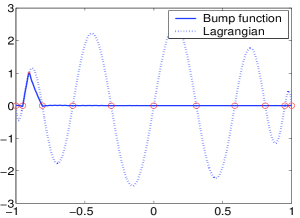
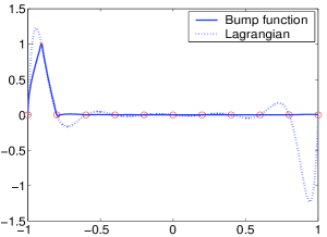
Figure 1: Bump functions and low-order Lagrangians for Chebyshev(left) and equidistant points

8.7 Kernel-Based Recovery Problems

The goal of this section is to include the Trade-off Principle of schaback:1995-1 as a special case, though it looks different, considering eigenvalues of kernel matrices there.

Assume a generalized interpolation using a set $\Lambda:=\{\lambda_{1},\ldots,\lambda_{N}\}$ of linearly independent functionals and the trial space $H_{\Lambda,K}:=\{\lambda^{x}K(x,\cdot)\;:\;\lambda\in\Lambda\}$ for a positive definite kernel $K$ on a set $\Omega$. The kernel matrix $A_{\Lambda,K}$ has entries

$$\lambda_{j}^{x}\lambda_{k}^{y}K(x,y)=(\lambda_{j},\lambda_{k})_{H_{K}^{*}},\;1\leq j,k\leq N$$

in the inner product of the dual $H_{K}^{*}$ of the native space $H_{K}$ for $K$ and is positive definite. By standard arguments from Optimal Recovery in Reproducing Kernel Hilbert Spaces, Theorem 2 holds, and we have a Trade-off Principle in the form (13) for Lagrangians with equality.

But the result of schaback:1995-1 looks different. To see the connection, recall that the squared Power Function for the add-one-in situation is the quadratic form

$$\left(\begin{array}[]{c}1\\ -\mu(u_{1})\\ \vdots\\ -\mu(u_{N})\end{array}\right)^{T}\left(\begin{array}[]{cccc}(\mu,\mu)&(\mu,\lambda_{1})&\ldots&(\mu,\lambda_{N})\\ (\lambda_{1},\mu)&(\lambda_{1},\lambda_{1})&\ldots&(\lambda_{1},\lambda_{N})\\ \vdots&\vdots&\ddots&\vdots\\ (\lambda_{N},\mu)&(\lambda_{N},\lambda_{1})&\ldots&(\lambda_{N},\lambda_{N})\\ \end{array}\right)\left(\begin{array}[]{c}1\\ -\mu(u_{1})\\ \vdots\\ -\mu(u_{N})\end{array}\right)$$

where the $u_{j}$ are the Lagrangians. The proof of the trade-off principle in schaback:1995-1 proceeds via the smallest eigenvalue of the matrix and ignores norms of Lagrangians. Furthermore, it is just an inequality in its original form, while Theorem 2 yields an equation and is much more general.

To see how schaback:1995-1 could have proven equality in (13) more than 25 years earlier, we look at the connection now. This requires to identify the quadratic form with the reciprocal of $\|u_{\mu,\Lambda}\|_{U}^{2}$. Consider the function $u$ based on the extended set of functionals and with coefficients $(1,-\mu(u_{1}),\ldots,-\mu(u_{N}))^{T}$. Then the matrix-vector product above gives the data, and the quadratic form above is the $U$-norm squared. The function is

$$u(x)=\mu^{y}K(y,x)-\sum_{j}\mu(u_{j})\lambda^{y}_{j}K(y,x),$$

and it is the function where the alternative form

$$P_{a_{\Lambda}}(\mu)=\sup_{\|u\|_{U}\leq 1,\Lambda(u)=0}\mu(f)$$

of the Power function attains its supremum, up to a factor DeMarchi-et-al:2005-1 . Thus $\Lambda(u)=0$ and

$$P_{a_{\Lambda}}(\mu)=\dfrac{\mu(u)}{\|u\|_{U}}.$$

But the above discussion shows that $P^{2}_{a_{\Lambda}}(\mu)=\|u\|_{U}^{2}$, proving $\mu(u)=P^{2}_{a_{\Lambda}}(\mu)$. This implies $u=P^{2}_{a_{\Lambda}}(\mu)u_{\mu,\Lambda}$ and

$$P_{a_{\Lambda}}(\mu)^{2}=\|u\|_{U}^{2}=P^{4}_{a_{\Lambda}}(\mu)\|u_{\mu,\Lambda}\|_{U}^{2}$$

to arrive finally at the Trade-off Principle in the form

$$1=P^{2}_{a_{\Lambda}}(\mu)\|u_{\mu,\Lambda}\|_{U}^{2}.$$

Remark: As long as the recovery map $a_{\Lambda}$, the evaluation functionals and the chosen space $U$ are fixed, there is no escape from the Trade-off Principle in the above form by changes of bases, because both ingredients are basis-independent. This is in sharp contrast to the widespread opinion that basis changes help. The observed large conditions of kernel matrices are a consequence of the small Power Functions for the chosen spaces. But by changing the recovery strategy, one can sacrifice small errors for better evaluation stability. Sections 9.1 and 11 will provide examples.

Remark: Once the functionals are fixed, one can vary the kernel, with respect to smoothness and scale. The Trade-off Principle will hold as an equality in all cases.

9 Unsymmetric Case

The previous two sections still used interpolation and Lagrangians. But there are much more general cases, e.g. for PDE solving by unsymmetric meshless methods. In the latter case, users have no freedom to choose the data functionals, because they are prescribed by the PDE to be solved. The functionals will generate boundary values or values of the differential operator in the interior. We further assume that the user prefers a certain sort of trial functions that should finally approximate the true PDE solution very well. In cases with well-posedness in the sense of Real Analysis, it suffices to come up with such a solution even if there is no uniqueness of the recovery procedure schaback:2016-4 .

Before we look at the trial space, recall that optimal Power Functions are purely dual objects,

$$P_{\Lambda}(\mu)=\min_{a\in\mathbb{R}^{\lvert\Lambda\rvert}}\|\mu-\sum_{\lambda\in\Lambda}a_{\lambda}\lambda\|_{U^{*}},$$

not depending on trial spaces, and will always outperform other solutions, error-wise. Norm-minimal bump functions will also not be dependent on trial spaces. and if restricted to some trial space, their norm will not be minimal. In view of a Trade-off Principle, this means that non-optimal recovery methods will sacrifice smaller errors for larger stability.

Anyway, we now consider a set $\Lambda$ of data functionals $\lambda_{1},\ldots,\lambda_{M}$ and set of trial functions $v_{1},\ldots,v_{N}$ from some normed space $U$ of functions, spanning a subspace $V$. These two ingredients determine a generalized Vandermonde matrix $A_{\Lambda,V}$ of size $M\times N$ with entries $\lambda_{j}(v_{k})$ that is in the theoretical background, though certain algorithms will never generate it as a whole. We also assume that there may be an unknown numerical rank that limits the practical use of the matrix as is. This occurs in plenty of kernel-based methods, and even in square cases $M=N$ there may be a rank loss that occurs while the matrix condition in the sense of MATLAB’s condest is still tolerable.

There are many ways to deal with this situation, and here we assume that the practically applied technique uses an $N\times M$ matrix $C$ that calculates coefficients for the trial space basis for a given data vector $\Lambda(f)$. By an $N$-vector $v$ of the $N$ basis functions, the result is a function $v^{T}C\Lambda(f)$, and evaluation of a functional $\mu$ has the error

$$\mu(f)-\mu(v)^{T}C\Lambda(f)=\mu(f)-\sum_{j=1}^{N}\mu(v_{j})\sum_{k=1}^{M}C_{jk}\lambda_{k}(f)=\mu(f)-\sum_{k=1}^{M}\mu(a_{k})\lambda_{k}(f)$$ (16)

for pseudo-Lagrangians

$$a_{k}=\displaystyle{\sum_{j=1}^{N}v_{j}C_{jk}},\,1\leq k\leq M$$ (17)

leading to the Power Function being the dual norm

$$P_{\Lambda,C}(\mu)=\left\|\mu-\sum_{j=1}^{N}\mu(v_{j})\sum_{k=1}^{M}C_{jk}\lambda_{k}\right\|_{U^{*}}.$$ (18)

Bump functions are not necessarily connected to the trial space chosen. If there exists a bump function $f_{\mu,\Lambda}$, the Trade-off Principle (10) applies for the above Power Function. The next section will treat a special case in more detail, because it has a huge background literature in applications.

9.1 Unsymmetric Collocation

An important example for solving PDEs via a recovery of functions is unsymmetric collocation, named after Edward Kansa kansa:1986-1 . Here, we confine ourselves to a standard Poisson problem (3) discretized as (4) for simplicity. One chooses a reproducing kernel Hilbert space ${\cal{H}}$ of functions on $\Omega$ that matches the expectable smoothness of the solution, and implements the PDE via test functionals, as sketched in Section 2. The functionals in (4) may be renamed as $\lambda_{m},1\leq m\leq M:=M_{\Delta}+M_{\beta}$ to match the notations used above. But note that $M$ will usually exceed $N$.

Symmetric collocation takes a space of trial functions where these test functionals act on the kernel $K$, and this is an optimal recovery strategy schaback:2015-3 in the space ${\cal{H}}$, with good convergence properties franke-schaback:1998-1 franke-schaback:1998-2a . The trade-off principle for this was treated in section 8.7.

The unsymmetric approach takes a set of trial functionals $\tau_{k}=\delta_{z_{k}},\;1\leq k\leq N$ to generate trial functions

$$v_{k}(x)=\tau_{k}^{y}K(y,x)=K(z_{k},x),\;1\leq k\leq N,\;x\in\overline{\Omega}.$$

The notation is now like in sections 8.6 and 9, but we have not yet specified how we choose the matrix $C$ of (16).

For calculation of the Power Function, we use (16), define the pseudo-Lagrangians $a_{k}$ from (17) and get

$$\begin{array}[]{rcl}P_{\Lambda,C}^{2}(\mu)&=&(\mu-\sum_{k}\mu(a_{k})\lambda_{k},\mu-\sum_{k}\mu(a_{k})\lambda_{k})_{U^{*}}\\ &=&K_{\mu,\mu}-2b^{T}K_{\Lambda,\mu}+b^{T}K_{\Lambda,\Lambda}b\end{array}$$

in self-evident kernel matrix notation and $b=\mu(a)=\mu(C^{T}v)$. The Power Function for symmetric collocation replaces $b$ by the solution $b^{*}$ of the system $K_{\Lambda,\Lambda}b=K_{\Lambda,\mu}$ and therefore realizes the minimum of the quadratic form over all possible vectors $b$.

Figure 2 shows squares of Power Functions for unsymmetric collocation of a Poisson problem with Dirichlet data on the unit square. The setting has 121 regular interior points, 16 regular boundary points, 121 regular trial points and uses a Matern-Sobolev kernel of order 5 at scale 1. The matrix $C$ was the pseudoinverse of the generalized Vandermonde matrix $A_{\Lambda,V}$.

The corresponding squares of optimal Power Functions from symmetric collocation are in Figure 3. They are not substantially smaller, just by a factor of about $1/2$.

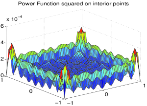
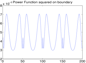
Figure 2: Squares of Power Functions in interior and on boundary, for unsymmetric collocation

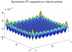
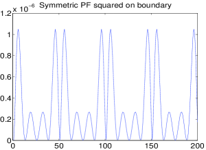
Figure 3: Squares of optimal Power Functions in interior and on boundary, for symmetric collocation

Norm-minimal bump functions exist and have norms that are related to the optimal Power Function via Theorem 2 by equality in (12) and (13). They are Lagrangians for the symmetric setting. Therefore the right-hand sides of these inequalities get larger when the Power Function $P_{\Lambda,C}$ is inserted. The reciprocals of squared norms of the optimal bump functions are visualized in Figure 3, because they coincide with the square of the optimal Power Function. Special bump functions in the trial space of the unsymmetric case will usually not exist if $M>N$.

But it may be an advantage of the unsymmetric technique that its evaluation is based on pseudo-Lagrangians instead of Lagrangians.

The columns of $C$ have the coefficients of the pseudo-Lagrangians $a_{k}$ in the trial basis, and therefore their squared norms $\|a_{k}\|_{U}^{2}$ are in the diagonal of the matrix $C^{T}K_{T,T}C$ where $K_{TT}$ is the standard kernel matrix for evaluations in trial points DeMarchi-et-al:2005-1 . Figure 4 shows the reciprocals of these, in order to compare with the squared optimal Power Functions in Figure 3. These results come out only on the data locations, without any plotting refinement. The values are larger by about a factor of 18 than those of the square of the optimal Power Function, indicating that the squared norms of the pseudo-Lagrangians are smaller than those of the Lagrangians for the symmetric case by a factor of $1/18$.

Summarizing, unsymmetric collocation works at a larger error level than symmetric collocation, but gets better evaluation stability by using pseudo-Lagrangians.

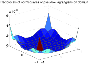
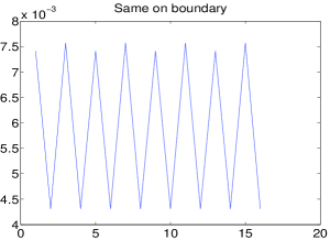
Figure 4: Reciprocals of squares of norms of Pseudo-Lagrangians in interior and on boundary

9.2 Non-square Linear Systems

Assume an overdetermined linear system $Ax\approx b$ with an $M\times N$ matrix $A$. The spaces $U$ and $U^{*}$ then are $\mathbb{R}^{M}$. After a Singular Value Decomposition, the new $M\times N$ system is $\Sigma y\approx c$ where the diagonal of $\Sigma$ carries the $N\leq M$ nonnegative singular values $\sigma_{j},\;1\leq j\leq N$. Formally, we set the $\sigma_{j},\;N<j\leq M$ to zero. Then

$$\begin{array}[]{rclll}\lambda_{k}(y)&=&\sigma_{k}y_{k},&\hbox{ for }\sigma_{k}>0,&\hbox{ else }=0\\ c_{jk}&=&\dfrac{\delta_{jk}}{\sigma_{k}},&\hbox{ for }\sigma_{k}>0,&\hbox{ else }=0\\ \end{array}$$

if there is no regularization for small $\sigma_{k}$. By some elementary Linear Algebra,

$$P^{2}_{\Lambda,C}(\mu)=\displaystyle{\sum_{\sigma_{k}=0}\mu_{k}^{2}}.$$

All bump vectors $f_{\mu,\Lambda}$ satisfy $f_{k}=0$ for $\sigma_{k}>0$ and

$$1=\mu(f)=\sum_{\sigma_{k}=0}\mu_{k}f_{k}$$

leading to the Trade-off Principle

$$1\leq P^{2}_{\Lambda,C}(\mu)\|f_{\mu,\Lambda}\|_{2}^{2}$$

that takes the classical form (8) here. If a Tikhonov-type regularization uses

$$c_{jk}(\tau)=\dfrac{\delta_{jk}}{\sigma_{k}+\tau}\hbox{ for all }k,$$

the bump functions stay the same, but the Power Function increases to

$$P^{2}_{\Lambda,C(\tau)}(\mu)=\displaystyle{\sum_{k}\mu_{k}^{2}\dfrac{\tau^{2}}{(\sigma_{k}+\tau)^{2}}}.$$

In the square nonsingular case, the Power Function is zero and there are no bump functions, leading back to the excluded $1\leq 0\cdot\infty$ situation.

10 Greedy Methods

Assume the add-one-in situation, and consider an optimal $\mu$ to be added to $\Lambda$ for an extended problem. In view of the Trade-off Principle, one should either take $\mu$ to maximize $P_{a_{\Lambda}}(\mu)$ or to minimize $f_{\mu,\Lambda}$. In cases satisfying Theorem 2, these strategies coincide. This aims at good stability and uses new functionals that cope with the current maximal error to make it zero in the next step. For interpolation of function values by polynomials, this leads to Leja points (leja:1957-1 , see also the survey by St. De Marchi demarchi:2004-1 ), while for kernel-based interpolation this is the $P$-greedy method of DeMarchi-et-al:2005-1 . Under certain additional assumptions, these strategies are approximately optimal in the sense that they realize $N$-widths (G. Santin and B. Haasdonk santin-haasdonk:2017-1 ), i.e. they generate trial spaces that are asymptotically optimal under all other trial spaces of the same dimension. They can be combined with the construction of Newton bases on-the-fly mueller-schaback:2009-1 , but we omit further details.

11 Outlook and Open Problems

The technique used in this paper is very elementary, and it is possible that there are earlier results on Trade-off Principles. On instance is platte-et-al:2010-2 by R. Platte et.al. proving instability of exponentially converging approximations to analytic functions. This paper proves in general that all convergence rates have at least their exact counterpart in rates of evaluation instability when using dual norms.

There are many more cases that fit into this paper, e.g. $h/p$ Finite Elements or spaces of multivariate splines. If errors are decreased by extended smoothness properties, there always will be an increasing evaluation instability. The connection between smoothness properties and convergence rates is a well-known Trade-off Principle in Approximation Theory, holding for several important cases, but a general theory seems to be lacking.

The same holds for a hypothetical Trade-off Principle suggesting that strongly localized methods cannot have small errors and/or large smoothness.

Handling the non-dual case is an open problem as well, in particular for $L_{\infty}$ evaluation stability.

If users have strong reasons to insist on very good accuracy and on evaluations of high derivatives, they have to face serious evaluation instabilities. Then it is a challenge to cope with these, including regularizations and other changes to the recovery map $a_{\Lambda}$. The literature on kernel-based methods provides several of such techniques, e.g. Contour-Padé fornberg-wright:2004-1 , RBF-QR fornberg-et-al:2011-1 , and RBF-GA fornberg-et-al:2013-1 by the group around Bengt Fornberg, and Hilbert-Schmidt-SVD by Fasshauer/McCourt (fasshauer-mccourt:2015-1, , Chapter 13). Greedy methods from Section 10 fight evaluation instability by choosing functionals or evaluation points adaptively.

Acknowledgement: The author is grateful to C.S. Chen of of the University of Southern Mississippi and Amir Noorizadegan of the National Taiwan University for an e-mail conversation that put evaluation instability into the focus for the Trade-off Principle.

References

- \bibcommenthead
- (1) Schaback, R.: Error estimates and condition numbers for radial basis function interpolation. Advances in Computational Mathematics, 251–264 (1995). https://doi.org/%****␣SEiLI.tex␣Line␣1625␣****10.1007/BF02432002
- (2) Wendland, H.: Scattered Data Approximation, p. 394. Cambridge University Press, Cambridge,UK (2005). https://doi.org/10.1017/CBO9780511617539
- (3) Fasshauer, G., McCourt, M.: Kernel-based Approximation Methods Using MATLAB. Interdisciplinary Mathematical Sciences, vol. 19. World Scientific, Singapore (2015). https://doi.org/10.1142/9335
- (4) Berrut, J.P., Trefethen, L.N.: Barycentric Lagrange interpolation. SIAM Review 46, 501–517 (2004). https://doi.org/10.1137/S0036144502417715
- (5) Schaback, R.: All well–posed problems have uniformly stable and convergent discretizations. Numerische Mathematik 132, 597–630 (2016). https://doi.org/10.1007/s00211-015-0731-8
- (6) Atluri, S.N., Zhu, T.-L.: A new meshless local Petrov-Galerkin (MLPG) approach to nonlinear problems in Computer modeling and simulation. Computer Modeling and Simulation in Engineering 3, 187–196 (1998)
- (7) Atluri, S.N., Zhu, T.-L.: A new meshless local Petrov-Galerkin (MLPG) approach in Computational Mechanics. Computational Mechanics (1998). https://doi.org/10.1007/s004660050346
- (8) Babuška, I., Banerjee, U., Osborn, J.E.: Survey of meshless and generalized finite element methods: a unified approach. Acta Numer. 12, 1–125 (2003). https://doi.org/10.1017/S0962492902000090
- (9) Farwig, R.: Multivariate interpolation of arbitrarily spaced data by moving least squares methods. J. Comp. Appl. Math. 16, 79–93 (1986). https://doi.org/10.1016/0377-0427(86)90175-5
- (10) Levin, D.: The approximation power of moving least-squares. Mathematics of Computation 67, 1517–1531 (1998). https://doi.org/10.1090/S0025-5718-98-00974-0
- (11) Wendland, H.: Local polynomial reproduction and moving least squares approximation. IMA Journal of Numerical Analysis 21, 285–300 (2001). https://doi.org/10.1093/imanum/21.1.285
- (12) Armentano, M.G.: Error estimates in Sobolev spaces for moving least square approximations. SIAM J. Numer. Anal. 39(1), 38–51 (2001). https://doi.org/10.1137/S0036142999361608
- (13) Belytschko, T., Krongauz, Y., Organ, D.J., Fleming, M., Krysl, P.: Meshless methods: an overview and recent developments. Computer Methods in Applied Mechanics and Engineering, special issue 139, 3–47 (1996). https://doi.org/10.1016/S0045-7825(96)01078-X
- (14) Mirzaei, D., Schaback, R., Dehghan, M.: On generalized moving least squares and diffuse derivatives. IMA J. Numer. Anal. 32 No. 3, 983–1000 (2012). https://doi.org/10.1093/imanum/drr030
- (15) Mirzaei, D., Schaback, R.: Direct Meshless Local Petrov-Galerkin (DMLPG) method: A generalized MLS approximation. Applied Numerical Mathematics 68, 73–82 (2013). https://doi.org/%****␣SEiLI.tex␣Line␣1825␣****10.1016/j.apnum.2013.01.002
- (16) Schaback, R.: A computational tool for comparing all linear PDE solvers. Advances of Computational Mathematics 41, 333–355 (2015). https://doi.org/10.1007/s10444-014-9360-5
- (17) Buhmann, M.D.: Radial Basis Functions, Theory and Implementations, p. 270. Cambridge University Press, Cambridge,UK (2003). https://doi.org/10.1017/CBO9780511543241
- (18) Schaback, R., Wendland, H.: Kernel techniques: from machine learning to meshless methods. Acta Numerica 15, 543–639 (2006). https://doi.org/10.1017/S0962492906270016
- (19) De Marchi, S., Schaback, R.: Stability of kernel-based interpolation. Adv. in Comp. Math. 32, 155–161 (2010). https://doi.org/10.1007/s10444-008-9093-4
- (20) Ahlberg, J.H., Nilson, E.N., Walsh, J.L.: The Theory of Splines and Their Applications. Mathematics in science and engineering, vol. 38. Academic Press, New York, N.Y. (1967). ISBN 0120447509, 9780120447503
- (21) Zwicknagl, B., Schaback, R.: Interpolation and approximation in Taylor spaces. Journal of Approximation Theory 171, 65–83 (2013). https://doi.org/10.1016/j.jat.2013.03.006
- (22) Driscoll, T.A., Hale, N., Trefethen, L.N.: Chebfun Guide. Pafnuty Publications, Oxford, UK (2014)
- (23) De Marchi, S., Schaback, R., Wendland, H.: Near-optimal data-independent point locations for radial basis function interpolation. Adv. Comput. Math. 23(3), 317–330 (2005). https://doi.org/10.1007/s10444-004-1829-1
- (24) Kansa, E.J.: Application of Hardy’s multiquadric interpolation to hydrodynamics. In: Proc. 1986 Simul. Conf., Vol. 4, pp. 111–117 (1986)
- (25) Franke, C., Schaback, R.: Solving partial differential equations by collocation using radial basis functions. Appl. Math. Comp. 93, 73–82 (1998). https://doi.org/10.1016/S0096-3003(97)10104-7
- (26) Franke, C., Schaback, R.: Convergence order estimates of meshless collocation methods using radial basis functions. Advances in Computational Mathematics 8, 381–399 (1998). https://doi.org/10.1023/A:1018916902176
- (27) Leja, F.: Sur certaines suits lièes aux ensemble plan et leur application á la representation conforme. Annales Polonici Mathematici 4, 8–13 (1957)
- (28) De Marchi, S.: On Leja sequences: some results and applications. Appl. Math. Comput. 152, 621–647 (2004). https://doi.org/10.1016/S0096-3003(03)00580-0
- (29) Santin, G., Haasdonk, B.: Convergence rate of the data-independent -greedy algorithm in kernel-based approximation. Dolomites Res. Notes Approx. 10(Special Issue), 68–78 (2017). https://doi.org/10.14658/pupj-drna-2017-Special_Issue-9
- (30) Müller, S., Schaback, R.: A Newton basis for kernel spaces. Journal of Approximation Theory 161, 645–655 (2009). https://doi.org/10.1016/j.jat.2008.10.014
- (31) Platte, R., Trefethen, L.N., Kuijlaars, B.J.: Impossibility of fast stable approximation of analytic functions from equispaced samples, 308–313 (2012). https://doi.org/10.1137/090774707. SIAM Review
- (32) Fornberg, B., Wright, G.: Stable computation of multiquadric interpolants for all values of the shape parameter. Comput. Math. Appl. 48(5-6), 853–867 (2004). https://doi.org/10.1016/j.camwa.2003.08.010
- (33) Fornberg, B., Larsson, E., Flyer, N.: Stable computations with Gaussian radial basis functions. SIAM J. Sci. Comput. 33(2), 869–892 (2011). https://doi.org/10.1137/09076756X
- (34) Fornberg, B., Lehto, E., Powell, C.: Stable calculation of Gaussian-based RBF-FD stencils. Computers and Mathematics with Applications 65, 627–637 (2013). https://doi.org/10.1016/j.camwa.2012.11.006