Concave likelihood-based regression with finite-support response variables

Abstract

We propose a unified framework for likelihood-based regression modeling when the response variable has finite support. Our work is motivated by the fact that, in practice, observed data are discrete and bounded. The proposed methods assume a model which includes models previously considered for interval-censored variables with log-concave distributions as special cases. The resulting log-likelihood is concave, which we use to establish asymptotic normality of its maximizer as the number of observations $n$ tends to infinity with the number of parameters $d$ fixed, and rates of convergence of $L_{1}$-regularized estimators when the true parameter vector is sparse and $d$ and $n$ both tend to infinity with $\log(d)/n\to 0$. We consider an inexact proximal Newton algorithm for computing estimates and give theoretical guarantees for its convergence. The range of possible applications is wide, including but not limited to survival analysis in discrete time, the modeling of outcomes on scored surveys and questionnaires, and, more generally, interval-censored regression. The applicability and usefulness of the proposed methods are illustrated in simulations and data examples.

1 Introduction

In practice observed data are discrete and bounded, be it by design, because of limited measurement precision, or because the data are stored in finite precision, for example as floating point numbers in a computer. However, it is common to ignore this and use models assuming continuous distributions, or continuous models for short. In general this practice leads to misspecification and biased estimators. While the bias can be small in some settings, it can be substantial in others, and the practice nevertheless persists. In our experience, this is in part due to a lack of reliable methods for the correctly specified likelihood and an unawareness of the potential pitfalls. To address these issues, we propose methods with theoretical and computational guarantees for a flexible class of regression models for finite-support (i.e., discrete and bounded) response variables. In addition, we illustrate the bias that can result from incorrectly applying a continuous model using simulations.

We consider four data examples, two of which are provided as Supporting Information. Each example is in a different setting with different challenges. Given the ubiquitous use of continuous models with data with finite support, the examples can illustrate but a small fraction of the many potential applications for the proposed methods. The first data example (Section 6.1) focuses on the effects of clinical predictors on plasma lipoprotein(a) [Lp(a)] levels measured in clinical care. Lp(a) is measured with finite precision, has a lower limit of detection, and a natural upper bound. Thus, in practice Lp(a) has finite support.

In the second example, cancer patients are observed repeatedly over the course of a study. For each patient, the time to death or distant metastases is recorded. Interest can be in univariable modeling of the time-to-event or, as is the focus in Section 6.2, the effects of clinical predictors and prediction using gene expressions. Either way, time-to-event has finite support: patients do not live forever, and time is measured with finite precision. Additionally, in many studies patients can be observed only at a few specific time points, leading to the observable time-to-event being far from continuous.

The third example (Web Appendix A.1) has an ordinal response, the total score on a depression screening questionnaire, taking values in $\{0,1,\dots,27\}$, and illustrates how the proposed methods can be used in settings where there need not exist a latent continuous variable of interest. The fourth example (Web Appendix A.2) focuses on discovering genes that predict, or are associated with, glucose intolerance. The response is ordinal with three levels and the number of predictors is three orders of magnitude larger than the number of observations.

Now, regardless of application, any response variable $Y$ with finite support $\mathcal{Y}$ can be modeled using the categorical distribution parameterized by the category probabilities. When the number of categories, that is, the cardinality of $\mathcal{Y}$, is small relative to the number of observations, it may be possible to estimate those probabilities with acceptable precision using the corresponding sample proportions. However, when the number of categories is large, their probabilities depend on predictors, or there is a known relation between the probabilities, then further modeling is often needed. We consider a model which handles many practically relevant settings and which leads to estimators with theoretical support. Specifically, we assume the probability mass function for $Y$ given a non-stochastic predictor vector $\bm{x}\in\mathbb{R}^{p}$ can be expressed, for functions $a$ and $b$ to be specified, as

$$f_{{\bm{\theta}}}(y\mid\bm{x})=\int_{a(y,\bm{x},{\bm{\theta}})}^{b(y,\bm{x},{\bm{\theta}})}r(w)\,\mathrm{d}w=R\{b(y,\bm{x},{\bm{\theta}})\}-R\{a(y,\bm{x},{\bm{\theta}})\},$$ (1)

where $r$ is a log-concave Lebesgue-density on $\mathbb{R}$, $R$ the corresponding cumulative distribution function, and ${\bm{\theta}}$ a parameter vector. We will assume $a$ and $b$ are affine in $\bm{\theta}$ for every $(y,\bm{x})$ and give further details on the specification in Section 2.

Intuitively (1) can be understood as the mass function for an interval-censored latent, continuous random variable $W$ with density $r$. In some settings $W$ has a practical interpretation. For example, it is typically related to the unobservable continuous time-to-event in settings such as the cancer study discussed above. On the other hand, (1) is also useful in many settings where there is no latent variable of practical interest. In fact, Example 1 establishes that, when there are no predictors, any mass function for a categorical random variable can be obtained as a special case of (1).

Authors considering models like (1) include Burridge, (1981, 1982) who note that, in some cases of interest, the log-likelihood is concave. These and some related results are discussed in the review of methods for grouped data by Heitjan, (1989). At the time, much of the literature was concerned with adjusting methods for continuous data to address bias introduced by grouping. By contrast, the focus here is the development of methods based on the correct likelihood. Likelihood-based methods for settings related to ours include that by Finkelstein, (1986), who proposed a model for interval-censored failure time data. Gentleman and Geyer, (1994) gave statistical and computational guarantees for maximum likelihood estimates under interval-censoring of a non-parametric model for survival times, and Huang, (1996) provided convergence rates for maximum likelihood estimators in interval-censored proportional hazards models. More recently, Taraldsen, (2011) studied the special case of rounded exponential data in detail, Zeng et al., (2016) proposed methods for interval-censored survival times, Couso et al., (2017) discussed different coarsening processes, and Guillaume et al., (2017) proposed robust optimization methods for coarse data in an essentially non-parametric setting. Kowal and Canale, (2020) also proposed a non-parametric method, for integer-valued data, mentioning rounded data as a relevant special case. McGough et al., (2021) studied penalized regression for censored and truncated, but not interval-censored, data. Notably, many of the applications are in survival analysis, which is natural given that time is generally measured in discrete units. A thorough treatment of survival analysis in discrete time is given by Tutz and Schmid, (2016). Here, we consider a unified framework including some models for survival analysis as special cases.

While some special cases of (1), for example logistic regression (see Section 2) and cumulative probability models (Example 1), have been studied extensively, the general setting has not. We give intuitive conditions on the density $r$ and endpoints $a$ and $b$ which guarantee asymptotic normality of the maximum likelihood estimator when the number of observations $n$ grows with the number of parameters $d$ fixed. Essentially, an asymptotic rank condition on a model matrix and $r$ being continuously differentiable suffices. We also consider settings where $d$ tends to infinity with $\log(d)/n\to 0$, and give convergence rates for an $L_{1}$-regularized maximum likelihood estimator under a restricted eigenvalue condition on a model matrix and $r$ continuously differentiable. Finally, we establish the numerical convergence of an inexact proximal Newton algorithm under conditions similar to those ensuring statistical convergence.

2 Model

Let $\Theta\subseteq\mathbb{R}^{d}$ be a convex parameter set and suppose $Y_{1},\dots,Y_{n}$ are independent, each having a mass function consistent with Model 1:

$$f^{i}_{\bm{\theta}}(y_{i}\mid\bm{x}_{i})=\int_{a_{i}(y_{i},\bm{x}_{i},{\bm{\theta}})}^{b_{i}(y_{i},\bm{x}_{i},{\bm{\theta}})}r(w)\,\mathrm{d}w=R\{b_{i}(y_{i},\bm{x}_{i},{\bm{\theta}})\}-R\{a_{i}(y_{i},\bm{x}_{i},{\bm{\theta}})\},$$ (2)

where $\bm{x}_{i}\in\mathcal{X}\subseteq\mathbb{R}^{p}$. We will often write $f_{\bm{\theta}}(y_{i}\mid\bm{x})$ instead of $f^{i}_{\bm{\theta}}(y_{i}\mid\bm{x}_{i})$ for brevity. The support $\mathcal{Y}_{i}=\{y_{i}:f^{i}_{\bm{\theta}}(y_{i}\mid\bm{x})>0\}$ need not be the same for every $i$, but we will assume $\mathcal{Y}=\cup_{i=1}^{\infty}\mathcal{Y}_{i}$ is finite. Define $r(\infty)=r(-\infty)=R(-\infty)=0$ and $R(\infty)=1$.

We assume, for $\bm{Z}_{i}=\bm{Z}_{i}(y_{i},\bm{x}_{i})\in\mathbb{R}^{2\times d}$ and $\bm{m}_{i}=\bm{m}_{i}(y_{i},\bm{x}_{i})\in[-\infty,\infty]^{2}$ to be defined shortly, $[a_{i}(y_{i},\bm{x}_{i},\bm{\theta}),b_{i}(y_{i},\bm{x}_{i},\bm{\theta})]^{\mathsf{T}}=\bm{Z}_{i}\bm{\theta}+\bm{m}_{i}$. When writing $\bm{Z}_{i}$ and $\bm{m}_{i}$ for brevity, dependence on $(y_{i},\bm{x_{i}})$ is implicit. Denote the first and second element of $\bm{m}_{i}$ by, respectively, $m_{i}^{a}$ and $m_{i}^{b}$. Accordingly, denote the first and second row of $\bm{Z}_{i}$ by, respectively, $\bm{z}_{i}^{a}$ and $\bm{z}_{i}^{b}$. We assume that if $m_{i}^{a}(y_{i},\bm{x}_{i})=-\infty$ for some $y_{i}\in\mathcal{Y}_{i}$, then it holds for every $\bm{x}_{i}\in\mathcal{X}$; and, for those $y_{i}$, we let $\bm{z}_{i}^{a}(y_{i},\bm{x}_{i})=\bm{0}$ for every $\bm{x}_{i}\in\mathcal{X}$. Thus, whether $a_{i}(y_{i},\bm{x}_{i},\bm{\theta})$ is finite or not depends only on $y_{i}$. Similarly, if $m_{i}^{b}(y_{i},\bm{x}_{i})=\infty$ for some $y_{i}\in\mathcal{Y}_{i}$, then it holds for every $\bm{x}_{i}\in\mathcal{X}$; and $\bm{z}^{b}_{i}(y_{i},\bm{x}_{i})=\bm{0}$.

The following three examples illustrate definitions and connections to some common models. Example 1 shows that, when there are no predictors, any model for a categorical response is a special case of (1), while Examples 2 and 3 include predictors.

Example 1 (Cumulative probability models).

Consider a response $Y$ with $m$ possible values, without loss of generality $\mathcal{Y}=\{1,\dots,m\}$. A possible version of (1) assumes $f_{\bm{\theta}}(y)$ is defined by

$$\begin{aligned} &f_{\bm{\theta}}(1)=R(\theta_{1}),~{}~{}f_{\bm{\theta}}(2)=R(\theta_{2})-R(\theta_{1}),\dots,~{}~{}f_{\bm{\theta}}(m-1)=R(\theta_{m-1})-R(\theta_{m-2}),\\ &f_{\bm{\theta}}(m)=1-R(\theta_{m-1}),\end{aligned}$$ (3)

with parameter set $\Theta=\{\bm{\theta}\in\mathbb{R}^{m-1}:\theta_{j}\geq\theta_{j-1},j\in\{2,\dots,m-1\}\}$. In the notation of (1), without predictors, $a(y,\bm{\theta})=-\infty$ if $y=1$, and $a(y,\bm{\theta})=\theta_{y-1}$ otherwise. Similarly, $b(y,\bm{\theta})=\infty$ if $y=m$ and $b(y,\bm{\theta})=\theta_{y}$ otherwise. One may also write (3) as $\mathsf{P}_{\theta}(Y\leq j)=R(\theta_{j})$, $j\in\{1,\dots,m-1\}$, which shows cumulative probability models are a special case of (1); see e.g. Agresti, (2019, Section 6.2), who uses a different but equivalent parameterization. Because $R$ is continuous it is straightforward to show any vector of category probabilities $[f_{\bm{\theta}}(1),\dots,f_{\bm{\theta}}(m)]^{\mathsf{T}}$ is attainable as $\bm{\theta}$ varies in $\Theta$. Thus, any categorical distribution is a special case of (1). Lastly we note that, in this example, any choice of $R$ gives the same model, or set of distributions, $\{f_{\bm{\theta}}:\bm{\theta}\in\Theta\}$. This will in general not be the case when there are predictors as, then, $R$ determines how the predictors affect the probabilities.

Example 2 (Interval-censored regression).

Suppose for some $\sigma>0$, ${\bm{\beta}}\in\mathbb{R}^{p}$, and $W_{i}$ with log-concave Lebesgue-density $r$ on $\mathbb{R}$, independently for $i\in\{1,\dots,n\}$,

$$Y_{i}^{*}=\bm{x}_{i}^{\mathsf{T}}{\bm{\beta}}+\sigma W_{i}.$$ (4)

Suppose also, for some $k_{i}\geq 1$ and known cut points $-\infty=t_{0}^{i}<t_{1}^{i}<\cdots<t_{k_{i}}^{i}<t^{i}_{k_{i}+1}=\infty$, the observed response is

$$Y_{i}=\begin{cases}y_{i}^{(0)},&Y_{i}^{*}\in(t^{i}_{0},t^{i}_{1})\\ \vdots&\\ y_{i}^{(k_{i})},&Y_{i}^{*}\in[t_{k_{i}}^{i},t_{k_{i}+1}^{i})\end{cases},$$

where the interval labels $y^{(0)}_{i},\dots,y^{(k_{i})}_{i}$ are arbitrary. Common binary regression models such as probit and logistic regression are special cases with, for every $i$, $k_{i}=1$, $t^{i}_{1}=0$, known $\sigma=1$, and $W_{i}$ having standard normal or logistic distribution, respectively. More generally, in the parameterization ${\bm{\theta}}=[\sigma^{-1},\sigma^{-1}{\bm{\beta}}^{\mathsf{T}}]^{\mathsf{T}}\in\mathbb{R}^{p+1}$, for $j\in\{0,\dots,k\}$,

$$f_{\bm{\theta}}(y_{i}^{(j)}\mid\bm{x}_{i})=R([t_{j+1}^{i},-\bm{x}_{i}^{\mathsf{T}}]{\bm{\theta}})-R([t_{j}^{i},-\bm{x}_{i}^{\mathsf{T}}]{\bm{\theta}}),$$ (5)

which is consistent with (1). In particular, $a_{i}(y_{i},\bm{x}_{i},{\bm{\theta}})=-\infty$ if $y_{i}=y^{i}_{(0)}$ and, otherwise, $a_{i}(y_{i},\bm{x}_{i},{\bm{\theta}})={\bm{\theta}}^{\mathsf{T}}\bm{z}_{i}^{a}=\bm{\theta}^{\mathsf{T}}[t^{i}_{j},-\bm{x}_{i}^{\mathsf{T}}]^{\mathsf{T}}$ and $m_{i}^{a}=0$. Similarly, $b_{i}(y_{i},\bm{x}_{i},{\bm{\theta}})=\infty$ if $y_{i}=y_{i}^{(k)}$ and, otherwise, $b_{i}(y_{i},\bm{x}_{i},{\bm{\theta}})={\bm{\theta}}^{\mathsf{T}}\bm{z}_{i}^{b}={\bm{\theta}}^{\mathsf{T}}[t^{i}_{j+1},-\bm{x}_{i}^{\mathsf{T}}]^{\mathsf{T}}$ and $m^{b}_{i}=0$.

Without predictors, (5) is similar to (3). However, in (5) without predictors the arguments to $R$ are determined by the known cut points and one parameter, $\theta_{1}$, while in (3) the cut points are parameters.

Example 3 (Interval-censored flexible parametric survival models).

Royston and Parmar, (2002) introduce a class of flexible parametric models for survival analysis. One model assumes a survival time $T$ has cumulative distribution function $F(t;\bm{x},{\bm{\beta}},{\bm{\gamma}})=1-\exp[-\exp\{\mathtt{sp}(\log t;{\bm{\gamma}})-{\bm{\beta}}^{\mathsf{T}}\bm{x}\}],$ where $\mathtt{sp}(\log t;{\bm{\gamma}})$ is a spline of $\log(t)$ with coefficients ${\bm{\gamma}}$. Any $\mathtt{sp}(\cdot;{\bm{\gamma}})$ which is monotone increasing for every ${\bm{\gamma}}$ in the parameter set and tends to $\pm\infty$ when its argument does, gives a valid cumulative distribution function. The exponential distribution is a special case with $\mathtt{sp}(\log t;{\bm{\gamma}})=\log t$. In practice, what is observed is often an interval containing $T$, say

$$Y=\begin{cases}y^{(0)},&T\in[0,t_{1})\\ \vdots&\\ y^{(k)},&T\in[t_{k},\infty)\end{cases},$$

where $t_{0}=0<t_{1}<\cdots<t_{k}<\infty$ the observation subscript $i$ is suppressed for simplicity. Thus, for example, $f_{\bm{\theta}}(y^{(1)}\mid\bm{x})=F(t_{2};\bm{x},{\bm{\beta}},{\bm{\gamma}})-F(t_{1};\bm{x},{\bm{\beta}},{\bm{\gamma}})$. Using this it is straightforward to show the mass function for $Y$ satisfies (1) with $R(w)=1-\exp\{-\exp(w)\}$, ${\bm{\theta}}=[{\bm{\gamma}}^{\mathsf{T}},{\bm{\beta}}^{\mathsf{T}}]^{\mathsf{T}}$, and $\bm{z}^{a}$ and $\bm{z}^{b}$ defined accordingly.

Next we establish concavity of the log-likelihood. The log-likelihood for one observation is $\ell^{i}({\bm{\theta}};y_{i},\bm{x}_{i})=\log\{f_{\bm{\theta}}(y_{i}\mid\bm{x}_{i})\}$, and $\ell_{n}({\bm{\theta}};\bm{Y},\bm{X})=\sum_{i=1}^{n}\ell^{i}({\bm{\theta}};y_{i},\bm{x}_{i})$, where $\bm{Y}=[Y_{1},\dots,Y_{n}]^{\mathsf{T}}\in\mathbb{R}^{n}$ and $\bm{X}=[\bm{x}_{1},\dots,\bm{x}_{n}]^{\mathsf{T}}\in\mathbb{R}^{n\times p}$.

Theorem 2.1.

The log-likelihood $\ell_{n}(\cdot;\bm{Y},\bm{X})$ given by model (2) is concave on $\Theta$. Moreover, if $\sum_{i=1}^{n}\bm{Z}_{i}^{\mathsf{T}}\bm{Z}_{i}$ is positive definite and $r$ is strictly positive, strictly log-concave, and continuously differentiable; then $\ell_{n}(\cdot;\bm{Y},\bm{X})$ is strictly concave on every open, convex subset of $\Theta$.

The proof of Theorem 2.1 uses classical results on log-concave functions due to Prékopa, (1973) and is in the Supporting Information along with proofs of other formally stated results. A special case of the non-strict concavity given by Theorem 2.1 is discussed without proof by Burridge, (1982, p.150). We have not seen the strict part, which requires substantially more work, stated or proved before. The essential component in its proof is Lemma B.1 (Supporting Information) which establishes strict log-concavity of the map $(t_{1},t_{2})\mapsto\{R(t_{2})-R(t_{1})\}$. The strictness of that log-concavity is critical for our results with diverging number of parameters.

3 Asymptotic properties

3.1 Fixed number of parameters

We consider maximum likelihood estimators

$$\widehat{{\bm{\theta}}}_{n}\in\operatorname*{arg\,min}_{{\bm{\theta}}\in\Theta}G_{n}({\bm{\theta}};\bm{Y},\bm{X}),$$

where $G_{n}({\bm{\theta}};\bm{Y},\bm{X})=-n^{-1}\ell_{n}({\bm{\theta}};\bm{Y},\bm{X})$. Because $\ell_{n}(\cdot;\bm{Y},\bm{X})$ is concave on the convex $\Theta$ (Theorem 2.1), $\widehat{{\bm{\theta}}}_{n}$ is a solution to a stochastic convex optimization problem, which is used in the proofs of our main asymptotic results.

In results and their proofs $c_{j}\in(0,\infty)$, $j\in\{1,2,\dots\}$, denote generic constants which can change between statements but, in each statement, depend on neither of $i$, $n$, $d$, $\bm{Y}$, $\bm{X}$, or $\bm{\theta}$. We use $\|\cdot\|$ for the spectral norm for matrices and Euclidean norm for vectors, $\|\cdot\|_{\infty}$ for the max-norm (maximum absolute element), and $\|\cdot\|_{1}$ for the one-norm (sum of absolute elements). The true parameter is denoted $\bm{\theta}_{*}$.

The following assumption will be used in both the low- and high-dimensional settings.

Assumption 1.

For all small enough $\rho>0$, there is a compact $E\subseteq\{\bm{t}\in\mathbb{R}^{2}:t_{1}<t_{2}\}$ such that, for every $i\in\mathbb{N}=\{1,2,\dots\}$, $y_{i}\in\mathcal{Y}_{i}$, $\bm{x}_{i}\in\mathcal{X}$, and $\bm{\theta}\in\Theta$ with $\|\bm{\theta}-\bm{\theta}_{*}\|_{1}\leq\rho$, it holds that either $\bm{Z}_{i}\bm{\theta}+\bm{m}_{i}\in E$ or an element of $\bm{m}_{i}$ is infinite. Moreover, for some $c_{1}<\infty$, $\|\bm{Z}_{i}\|_{\infty}\leq c_{1}$ and, when the left-hand sides are finite, $|m_{i}^{a}|\leq c_{1}$ and $|m_{i}^{b}|\leq c_{1}$.

The particular choice of norms in Assumption 1 is unimportant when $d$ is fixed but will matter in later sections when $d\to\infty$. To get some intuition for the first part of the assumption, consider for example the interval-censored regression in Example 2. As noted following (5), when both $t_{j}^{i}$ and $t_{j+1}^{i}$ are finite, $\bm{m}_{i}=\bm{0}$ and $\bm{\theta}^{\mathsf{T}}\bm{z}_{i}^{a}=\sigma^{-1}t^{i}_{j}-\bm{x}_{i}^{\mathsf{T}}\bm{\beta}/\sigma<\sigma^{-1}t^{i}_{j+1}-\bm{x}_{i}^{\mathsf{T}}\bm{\beta}/\sigma$. Using this and that $\sigma_{*}>0$, it is straightforward to show Assumption 1 holds (see Proof of Corolloray 1, Supporting Information, for an example). More generally, Assumption 1 ensures among other things that the support does not depend on $\bm{\theta}$ near $\bm{\theta}_{*}$.

To state the first result, let $\lambda_{\min}(\cdot)$ denote the smallest eigenvalue of its matrix argument.

Theorem 3.1.

If (a) $\mathcal{Y}$ is finite, (b) $r$ is strictly log-concave, strictly positive, and continuously differentiable on $\mathbb{R}$; (c) ${\bm{\theta}}_{*}$ is an interior point of $\Theta$; (d) Assumption 1 holds; and (e)

$$\liminf_{n\to\infty}\lambda_{\min}\left\{\sum_{i=1}^{n}\mathbb{E}(\bm{Z}_{i}^{\mathsf{T}}\bm{Z}_{i})/n\right\}>0;$$ (6)

then as $n\to\infty$ with $d$ fixed, $\bm{\mathcal{I}}_{n}(\bm{\theta}_{*};\bm{X})^{1/2}(\widehat{{\bm{\theta}}}_{n}-{\bm{\theta}}_{*})\rightsquigarrow\mathcal{N}(\bm{0},\bm{I}_{d})$, where $\bm{\mathcal{I}}_{n}(\bm{\theta}_{*};\bm{X})=\operatorname{cov}\{\nabla\ell_{n}({\bm{\theta}}_{*};\bm{Y},\bm{X})\}$ is the Fisher information.

The proof of Theorem 3.1 uses a result by Hjort and Pollard, (2011) on minimizers of convex processes. The expectation and covariance in the theorem statement are with respect to the distribution of $\bm{Y}\mid\bm{X}$ under the true ${\bm{\theta}}_{*}$. In the proof it argued that $\bm{\mathcal{I}}_{n}(\bm{\theta};\bm{X})$ has eigenvalues bounded below by $\epsilon n$ for some $\epsilon>0$. With this, the theorem implies $\|\widehat{\bm{\theta}}_{n}-\bm{\theta}_{*}\|=O_{\mathsf{P}}(1/\sqrt{n})$. If $r$ is assumed to be twice continuously differentiable, then the conclusion of the theorem continues to hold if $\bm{\mathcal{I}}_{n}(\bm{\theta};\bm{X})$ is replaced by the observed information $-\nabla^{2}\ell_{n}(\bm{\widehat{\theta}}_{n};\bm{Y},\bm{X})$ (Theorem B.5, Supporting Information). In the case of interval-censored linear regression, (6) reduces to a familiar condition on the design matrix $\bm{X}=[\bm{x}_{1},\dots,\bm{x}_{n}]^{\mathsf{T}}\in\mathbb{R}^{n\times p}$.

Corollary 3.2.

Suppose $Y_{1},\dots Y_{n}$ satisfy the interval-censored regression model in Example 2 with known $\sigma=1$, $\mathcal{Y}$ is finite, the density of $W_{i}$ satisfies requirement (b) of Theorem 3.1, and $\|\bm{x}_{i}\|\leq c_{1}$; then the conclusion of Theorem 3.1 holds if $\liminf_{n\to\infty}\lambda_{\min}\{\bm{X}^{\mathsf{T}}\bm{X}/n\}>0$ as $n\to\infty$ with $d=p$ fixed.

When $k\geq 2$ in the setting of Corollary 3.2, we expect the conclusion can be shown to hold also when $\sigma$ is unknown. Intuitively, when the support of the response variables has cardinality greater than two, the variance need not be a function of the mean, and it may then be possible to estimate an additional parameter. By contrast, it is well-known $\sigma$ is unidentifiable in general in logistic and probit regression, which are special cases.

3.2 Diverging number of parameters

Our second main result gives convergence rates for maximum $L_{1}$-regularized likelihood estimators when $d$ tends to infinity with $n$ and ${\bm{\theta}}_{*}$ is sparse. Since $d$ varies ${\bm{\theta}}_{*}$ generally depends on $d$, but we suppress this in notation. We consider the penalized average negative log-likelihood defined for $\lambda_{n}\geq 0$ by $G^{\lambda}_{n}({\bm{\theta}};\bm{Y},\bm{X})=G_{n}({\bm{\theta}};\bm{Y},\bm{X})+\lambda_{n}\|{\bm{\theta}}\|_{1}$, and $\widehat{{\bm{\theta}}}_{n}^{\lambda}\in\operatorname*{arg\,min}_{{\bm{\theta}}\in\Theta}G_{n}^{\lambda}({\bm{\theta}};\bm{Y},\bm{X}).$ For any ${\bm{\theta}}\in\mathbb{R}^{d}$ and $S\subseteq\{1,\dots,d\}$, define ${\bm{\theta}}_{S}\in\mathbb{R}^{d}$ to equal ${\bm{\theta}}$ with the $j$th element set to zero if $j\notin S$, $j\in\{1,\dots,d\}$:

$$({\bm{\theta}}_{S})_{j}=\begin{cases}\theta_{j}&j\in S\\ 0&j\notin S\end{cases}.$$

We say ${\bm{\theta}}$ is $s$-sparse if ${\bm{\theta}}={\bm{\theta}}_{S}$ for some $S\subseteq\{1,\dots,d\}$ with cardinality $s=|S|$.

To state results, define the cone $\mathbb{C}(S)=\{{\bm{\theta}}\in\mathbb{R}^{d}:\|{\bm{\theta}}_{S^{c}}\|_{1}\leq 3\|{\bm{\theta}}_{S}\|_{1}\}$, where $S^{c}=\{1,\dots,d\}\setminus S$ and, hence, ${\bm{\theta}}_{S^{c}}={\bm{\theta}}-{\bm{\theta}}_{S}$. Intuitively, $\mathbb{C}(S)$ is a set of nearly-sparse ${\bm{\theta}}$ in the sense that the elements $\theta_{j},j\notin S$, are not too large compared with the $\theta_{j},j\in S$. Define also for any $\kappa>0$, $n$, and $d$ the set

$$\mathcal{C}_{\kappa,n,d}=\left\{(\bm{Y},\bm{X}):\inf_{{\bm{\theta}}\in\mathbb{C}(S):\|{\bm{\theta}}\|=1}\left\{{\bm{\theta}}^{\mathsf{T}}\left(\frac{1}{n}\sum_{i=1}^{n}\bm{Z}_{i}^{\mathsf{T}}\bm{Z}_{i}\right){\bm{\theta}}\right\}\geq\kappa\right\}.$$

We are ready to state the next result.

Theorem 3.3.

If (a) $\Theta$ is open, (b) $r$ is strictly log-concave, strictly positive, and continuously differentiable on $\mathbb{R}$; (c) ${\bm{\theta}}_{*}$ is $s$-sparse and $\|{\bm{\theta}}_{*}\|_{\infty}\leq c_{1}$; (d) Assumption 1 holds; and (e) $\lambda_{n}=c_{2}\log(d)/n\to 0$; then there are $c_{3},c_{4},c_{5}$ such that, for large enough $n$ and $d$, with probability at least $\mathsf{P}(\mathcal{C}_{\kappa,n,d})-d^{-c_{3}}$,

$$\|\widehat{{\bm{\theta}}}^{\lambda}_{n}-{\bm{\theta}}_{*}\|^{2}\leq c_{4}\frac{\log(d)}{n};\quad\|\widehat{{\bm{\theta}}}^{\lambda}_{n}-{\bm{\theta}}_{*}\|_{1}\leq c_{5}\sqrt{\frac{\log(d)}{n}}.$$

Assumptions (a) and (b) ensure the gradient and Hessian of $G_{n}$ exist. In some settings of interest, for example interval-censored regressions with known error variance, the matrices $\bm{Z}_{1},\dots,\bm{Z}_{n}$ do not depend on $\bm{Y}$. Then the event $\mathcal{C}_{\kappa,n,d}$ either contains all outcomes or none and is hence better thought of as a restricted eigenvalue condition on the deterministic $\sum_{i=1}^{n}\bm{Z}_{i}^{\mathsf{T}}\bm{Z}_{i}/n$. Specifically, if the inequality in the definition of $\mathcal{C}_{\kappa,n,d}$ holds for some $\kappa>0$ and all $n$ and $d$, and the other conditions of the theorem hold, then the conclusion of the theorem holds with probability at least $1-d^{-c_{3}}$. Moreover, in interval-censored regression with known error variance, a restricted eigenvalue condition on $\sum_{i=1}^{n}\bm{Z}_{i}^{\mathsf{T}}\bm{Z}_{i}/n$ is equivalent to one on $\bm{X}^{\mathsf{T}}\bm{X}/n$ since, in those cases, $\bm{Z}_{i}=-[\bm{x}_{i},\bm{x}_{i}]^{\mathsf{T}}$, with one of the rows replaced by zeros if $a_{i}(y_{i},\bm{x}_{i},{\bm{\theta}})=-\infty$ or $b_{i}(y_{i},\bm{x}_{i},{\bm{\theta}})=\infty$.

It is common in the literature for the bounds on norms of $\widehat{{\bm{\theta}}}^{\lambda}_{n}-{\bm{\theta}}_{*}$ to depend linearly on $s$ (e.g., Negahban et al.,, 2012, Corollary 2). Here, $s$ is fixed and absorbed in the constants $c_{4}$ and $c_{5}$. This is because our proofs require $\bm{Z}_{i}{\bm{\theta}}_{*}$ to be contained in a compact subset of $\mathbb{R}^{2}$. We expect the linear dependence on $s$ can be recovered in many special cases, though it may require substantial work; see for example Negahban et al., (2009) for the special case of logistic regression.

4 Computing

4.1 Inexact proximal Newton

We propose using an inexact proximal Newton algorithm for computing $\widehat{{\bm{\theta}}}^{\lambda}_{n}$ in practice. That is, a proximal Newton algorithm where the sub-problems are solved inexactly. Similar algorithms have proven useful in, for example, the fitting of penalized generalized linear models (Lee et al.,, 2006; Friedman et al.,, 2010; Yuan et al.,, 2012; Byrd et al.,, 2016). The R package fsnet (2022) implements the algorithm, and an accelerated proximal gradient descent algorithm similar to the Fast Iterative Shrinkage-Thresholding (FISTA) algorithm (Beck and Teboulle,, 2009). We focus on the proximal Newton algorithm here because we found it tends to perform well. It is often useful in practice to include a ridge penalty and hence we solve the convex elastic-net optimization problem

$$\min_{{\bm{\theta}}\in\Theta}\left\{G_{n}({\bm{\theta}};\bm{Y},\bm{X})+\lambda_{1}\|{\bm{\theta}}\|_{1}+\frac{\lambda_{2}}{2}\|{\bm{\theta}}\|^{2}\right\},$$ (7)

where $\lambda_{1}\geq 0$ and $\lambda_{2}\geq 0$ are user-specified penalty parameters. The setting in Section 3.2 is a special case with $\lambda_{2}=0$. If $\lambda_{2}>0$ the objective function is strongly convex and has a unique global minimizer. To simplify notation, let us suppress dependence on the data $(\bm{Y},\bm{X})$ for the remainder of the section and re-define $G_{n}^{\lambda}$ to include the ridge penalty. That is, $G_{n}^{\lambda}({\bm{\theta}})$ is the objective function in (7).

Proximal Newton solves (7) by iteratively updating and minimizing an $L_{1}$-penalized quadratic approximation of $G_{n}^{\lambda}$. To be more specific, let $Q(\cdot;{\bm{\theta}}^{k})$ denote a quadratic approximation of the differentiable part of $G_{n}^{\lambda}$ at the $k$th iterate ${\bm{\theta}}^{k}$, given by

$$Q({\bm{\theta}};{\bm{\theta}}^{k})=\{\nabla G_{n}({\bm{\theta}}^{k})+\lambda_{2}{\bm{\theta}}^{k}\}^{\mathsf{T}}{\bm{\theta}}+\frac{1}{2}({\bm{\theta}}-{\bm{\theta}}^{k})^{\mathsf{T}}\{\nabla^{2}G_{n}({\bm{\theta}}^{k})+\lambda_{2}\bm{I}_{d}\}({\bm{\theta}}-{\bm{\theta}}^{k}).$$

Then the $(k+1)$th iterate in the proximal Newton algorithm is

$${\bm{\theta}}^{k+1}\approx\operatorname*{arg\,min}_{{\bm{\theta}}\in\Theta}\left\{Q({\bm{\theta}};{\bm{\theta}}^{k})+\lambda_{1}\|{\bm{\theta}}\|_{1}\right\},$$ (8)

where $\approx$ indicates it is not necessary to solve the optimization problem exactly (see Section 4.3). The update (8) does not in general admit a closed form solution but can be solved efficiently to desired tolerance using coordinate descent.

4.2 Coordinate descent

To discuss the coordinate descent algorithm for (8), we assume $\Theta=\mathbb{R}^{d}$ for simplicity. Settings where some parameters need to be positive (e.g., to ensure monotonic splines in an interval-censored flexible parametric model) or not penalized (e.g., the error scale parameter in an interval-censored regression), could be treated by minor modifications and are supported in our software.

The $(l+1)$th iterate for the $j$th component in a coordinate descent algorithm for (8) is

$$\theta^{k,l+1}_{j}=\operatorname*{arg\,min}_{\theta_{j}\in\mathbb{R}}\{Q([\theta_{1}^{k,l+1},\dots,\theta_{j},\theta_{j+1}^{k,l},\dots,\theta_{d}^{k,l}]^{\mathsf{T}};\bm{\theta}^{k})+\lambda_{1}|\theta_{j}|\}.$$ (9)

This is a univariate $L_{1}$-penalized quadratic optimization problem which can be solved in closed form using the soft-thresholding operator. To be more specific, define $\bm{g}:\mathbb{R}^{2}\to\mathbb{R}^{2}$ and $\bm{H}:\mathbb{R}^{2}\to\mathbb{R}^{2\times 2}$ as, respectively, the gradient and Hessian of the map $(t_{1},t_{2})\mapsto\log\{R(t_{2})-R(t_{1})\}$, $-\infty<t_{1}<t_{2}<\infty$. Extend also $\bm{g}$ and $\bm{H}$ to include points where $t_{1}=-\infty$ by setting the first element of $\bm{g}$ and first row and column of $\bm{H}$ to zero at such points. Similarly, extend to points with $t_{2}=\infty$ by setting the second element of $\bm{g}$ and second row and column of $\bm{H}$ to zero at such points. Then

$$\nabla G_{n}({\bm{\theta}};\bm{Y},\bm{X})=-\frac{1}{n}\sum_{i=1}^{n}\bm{Z}_{i}^{\mathsf{T}}\bm{g}(\bm{Z}_{i}{\bm{\theta}}+\bm{m}_{i});~{}~{}\nabla^{2}G_{n}({\bm{\theta}};\bm{Y},\bm{X})=-\frac{1}{n}\sum_{i=1}^{n}\bm{Z}_{i}^{\mathsf{T}}\bm{H}(\bm{Z}_{i}{\bm{\theta}}+\bm{m}_{i})\bm{Z}_{i}.$$

Let $\bm{\eta}_{i}^{k}=\bm{Z}_{i}{\bm{\theta}}^{k}+\bm{m}_{i}$, $\bm{H}_{i}^{k}=\bm{H}(\bm{\eta}_{i}^{k})$, $\bm{g}_{i}^{k}=\bm{g}(\bm{\eta}_{i}^{k})$, and

$$\bm{\eta}_{i(j)}^{k,l}=\sum_{m<j}\bm{Z}_{i}^{m}\theta_{m}^{k,l+1}+\sum_{m>j}\bm{Z}_{i}^{m}\theta_{m}^{k,l}+\bm{m}_{i},$$

where $\bm{Z}_{i}^{m}$ is the $m$th column of $\bm{Z}_{i}$. Up to terms not depending on $\theta_{j}$, the objective function in (9) is

$$\frac{\theta_{j}}{n}\sum_{i=1}^{n}\{-(\bm{Z}_{i}^{j})^{\mathsf{T}}\bm{g}_{i}^{k}+\lambda_{2}\theta_{j}^{k}+(\bm{\eta}_{i}^{k}-\bm{\eta}_{i(j)}^{k,l})^{\mathsf{T}}\bm{H}_{i}^{k}\bm{Z}_{i}^{j}\}+\frac{\theta_{j}^{2}}{2n}\sum_{i=1}^{n}\{-(\bm{Z}_{i}^{j})^{\mathsf{T}}\bm{H}_{i}^{k}\bm{Z}_{i}^{j}+\lambda_{2}\}+\lambda_{1}|\theta_{j}|.$$

Using this, a routine calculation shows the minimizer in (9) is

$$\theta_{j}^{k,l+1}=\frac{\operatorname{soft}\left[-\frac{1}{n}\sum_{i=1}^{n}\{-(\bm{Z}_{i}^{j})^{\mathsf{T}}\bm{g}_{i}^{k}+\lambda_{2}\theta_{j}^{k}+(\bm{\eta}_{i}^{k}-\bm{\eta}_{i(j)}^{k,l})^{\mathsf{T}}\bm{H}_{i}^{k}\bm{Z}_{i}^{j}\},\lambda_{1}\right]}{\frac{1}{n}\sum_{i=1}^{n}\{-(\bm{Z}_{i}^{j})^{\mathsf{T}}\bm{H}_{i}^{k}\bm{Z}_{i}^{j}+\lambda_{2}\}},$$ (10)

where $\operatorname{soft}(x,\lambda)=\mathrm{sign}(x)\max\{|x|-\lambda,0\}$. Notably, $\bm{\eta}_{i(j)}^{k,l}$ is the only term that needs updating in the coordinate descent, making each step fast to compute.

The resulting algorithm is stated in Algorithm 1.

Algorithm 1 Proximal Newton with coordinate descent

1. Input $\lambda_{1}\geq 0,\lambda_{2}\geq 0$, ${\bm{\theta}}^{1}\in\mathbb{R}^{d}$

2. For $k=1,2,\dots$ until convergence:

   1. Let ${\bm{\theta}}^{k,1}={\bm{\theta}}^{k}$ and for $l=1,2,\dots$ until convergence, update $\theta^{k,l+1}_{j}$ iteratively for $j=1,\dots,d$ according to (10).

   2. Let ${\bm{\theta}}^{k,l}$ be the vector of final iterates from (a) and set ${\bm{\theta}}^{k+1}=(1-s){\bm{\theta}}^{k}+s{\bm{\theta}}^{k,l}$ with $s\in[0,1]$ selected by backtracking line-search.

3. Return final iterate ${\bm{\theta}}^{k+1}$ from 2.

4.3 Convergence

Convergence of Algorithm 1 can be guaranteed by selecting appropriate termination criteria for the inner coordinate descent algorithm (step 2 (a)) and the backtracking line-search (step 2 (b)). It will be convenient to characterize solutions to (7) using the function $\bm{J}:\Theta\to\mathbb{R}^{d}$ defined for $c_{1}>0$ by $\bm{J}({\bm{\theta}};c_{1})=\nabla G_{n}({\bm{\theta}})+\lambda_{2}{\bm{\theta}}-\mathcal{P}_{\lambda_{1}}\{\nabla G_{n}({\bm{\theta}})+\lambda_{2}{\bm{\theta}}-{\bm{\theta}}/c_{1}\},$ where $\mathcal{P}_{\lambda_{1}}$ is the elementwise projection onto $[-\lambda_{1},\lambda_{1}]$. Routine calculations show, for any $c_{1}>0$, $\bm{J}({\bm{\theta}};c_{1})=0$ if and only if $0$ is a sub-gradient of $G^{\lambda}_{n}$ at ${\bm{\theta}}$ (Milzarek and Ulbrich,, 2014; Byrd et al.,, 2016); that is, $\bm{J}({\bm{\theta}};c_{1})=0$ if and only if ${\bm{\theta}}$ is a solution to (7). Similarly, ${\bm{\theta}}$ is a solution to (8) if and only if $\bm{J}_{Q}({\bm{\theta}};c_{1},{\bm{\theta}}^{k})=0$, where

$$\bm{J}_{Q}({\bm{\theta}};c_{1},{\bm{\theta}}^{k}) =\nabla G_{n}({\bm{\theta}}^{k})+\lambda_{2}{\bm{\theta}}^{k}+\{\nabla^{2}G_{n}({\bm{\theta}}^{k})+\lambda_{2}\bm{I}_{d}\}({\bm{\theta}}-{\bm{\theta}}^{k})$$

$$\quad-\mathcal{P}_{\lambda_{1}}[\nabla G_{n}({\bm{\theta}}^{k})+\lambda_{2}{\bm{\theta}}^{k}+\{\nabla^{2}G_{n}({\bm{\theta}}^{k})+\lambda_{2}\bm{I}_{d}\}({\bm{\theta}}-{\bm{\theta}}^{k})-{\bm{\theta}}/c_{1}].$$

Following Byrd et al., (2016), the coordinate descent algorithm for (9) may be terminated when the $l$th coordinate descent iterate ${\bm{\theta}}^{k,l}=[\theta_{1}^{k,1},\dots,\theta_{d}^{k,l}]^{\mathsf{T}}$ satisfies, for a user-specified $c_{2}\in[0,1)$,

$$\|\bm{J}_{Q}({\bm{\theta}}^{k,l};{\bm{\theta}}^{k},c_{1})\|\leq c_{2}\|\bm{J}_{Q}({\bm{\theta}}^{k};{\bm{\theta}}^{k},c_{1})\|.$$ (11)

To specify a termination criterion for the line-search in step 2 (b), define a first-order approximation of $G_{n}^{\lambda}$ at ${\bm{\theta}}^{k}$ by

$$L_{n}^{\lambda}({\bm{\theta}};{\bm{\theta}}^{k})=G_{n}({\bm{\theta}}^{k})+0.5\lambda_{2}\|{\bm{\theta}}^{k}\|^{2}+\{\nabla G_{n}({\bm{\theta}}^{k})+\lambda_{2}{\bm{\theta}}^{k}\}^{\mathsf{T}}({\bm{\theta}}-{\bm{\theta}}_{k})+\lambda_{1}\|{\bm{\theta}}\|_{1}.$$

Given ${\bm{\theta}}^{k,l}$ satisfying (11), backtracking line-search starts with step-size $s=1$ and decreases until, for a user-specified $c_{3}\in(0,1/2)$,

$$G_{n}^{\lambda}({\bm{\theta}}^{k})-G_{n}^{\lambda}\{(1-s){\bm{\theta}}^{k}+s{\bm{\theta}}^{k,l}\}\geq c_{3}[L_{n}^{\lambda}({\bm{\theta}}^{k};{\bm{\theta}}^{k})-L_{n}^{\lambda}\{(1-s){\bm{\theta}}^{k}+s{\bm{\theta}}^{k,l};{\bm{\theta}}^{k}\}].$$ (12)

We are ready to state a convergence result for Algorithm 1.

Theorem 4.1.

If in Algorithm 1 convergence in step 2 (a) is determined using (11), the backtracking linesearch in step 2 (b) satisifes (12), $r$ is continuously differentiable, and either

• $r$ is strictly log-concave and strictly positive, $\sum_{i=1}^{n}\bm{Z}_{i}^{\mathsf{T}}\bm{Z}_{i}$ is positive definite, and $\inf_{{\bm{\theta}}\in\Theta}G^{\lambda}_{n}({\bm{\theta}})=G^{\lambda}_{n}(\widehat{{\bm{\theta}}})$ for some $\widehat{{\bm{\theta}}}\in\Theta$; or

• $\lambda_{2}>0$;

then the sequence $\{{\bm{\theta}}^{k}\}$ of iterates satisfies $\lim_{k\to\infty}\bm{J}({\bm{\theta}}^{k};c_{1})=0$.

Conditions (a) and (b) are used to show, among other things, the iterates $\{{\bm{\theta}}_{k}\}$ stay in a compact set. If this can be guaranteed by other means, some conditions can be weakened. For example, it is typically possible to relax the first two requirements in (a) if the gradient is Lipschitz-continuous and the Hessian in the quadratic approximation $Q({\bm{\theta}};{\bm{\theta}}^{k})$ is regularized to have eigenvalue bounded away from zero. Notably, we have had no convergence issues in simulations even when $\lambda_{2}=0$ and $\sum_{i=1}^{n}\bm{Z}_{i}^{\mathsf{T}}\bm{Z}_{i}$ is indefinite because $d>n$, as long as $\lambda_{1}>0$.

5 Numerical experiments

We illustrate the proposed methods in two interval-censored regression models (see Example 2). In the first, $W$ has the extreme-value distribution with cumulative distribution function $R(w)=1-\exp\{-\exp(w)\}$, and the number of predictors $p=3$ is smaller than the number of observations $n=100$. When $W$ has the extreme-value distribution in (4) and $\sigma=1$, $\exp(Y^{*})$ has the exponential distribution with mean $\exp(\bm{x}^{\mathsf{T}}{\bm{\theta}})$. This model is a special case of that in Example 3. It is also a special case of a gamma generalized linear model with logarithm link function, which we therefore include in comparisons. The observed response indicates whether $\exp(Y^{*})$ is in $[0,d),[d,2d),\dots,[kd,5)$, or $[5,\infty)$, where $d$ (the interval size) varies in the simulations and $k$ is the largest integer such that $kd<5$. Thus, a larger $d$ corresponds to more severe censoring. Because $Y^{*}$ is not observed, when fitting the generalized linear model we take the upper endpoints of the observed intervals, or $5+d$ if the interval is $[5,\infty)$, as responses.

In the second setting $W$ is normally distributed and $p=200>100=n$. The observed intervals are for $Y^{*}$ are $(-\infty,5),[5,-kd),\dots,[-d,0),[0,d),\dots,[kd,5),[5,\infty)$. We compare the estimates from Algorithm 1 with $\lambda_{2}=0$ to those from lasso regression using glmnet (Friedman et al.,, 2010). For both methods, the regularization parameter $\lambda_{1}$ is selected by 5-fold cross-validation. For our method, we select the $\lambda_{1}$ which minimizes the average out-of-sample misclassification rate. Here, the misclassification rate for one fold is the proportion of observations $(Y_{i},\bm{x}_{i})$ in that fold for which the predicted mean $\bm{x}_{i}^{\mathsf{T}}\widehat{{\bm{\theta}}}_{n}^{\lambda}$ of the $i$th unobservable response $Y_{i}^{*}$ is outside the observed interval.

The predictors are generated as centered and scaled realizations from a multivariate normal distribution with mean zero and a covariance matrix with $(i,j)$th element $0.5^{|i-j|}$. When $p=3$ we include an intercept so there are two jointly normal predictors in addition to the intercept. The true coefficient vector is ${\bm{\theta}}_{*}=[1,1/2,-1/2]^{\mathsf{T}}$ when $p=3$ and ${\bm{\theta}}_{*}=[1,1/2,-1/2,0,\dots,0]^{\mathsf{T}}$ when $p=200$.

Figure 1 shows how sum of squared estimation errors for the non-zero components of ${\bm{\theta}}_{*}$ and mean misclassification rates vary with the interval size $d$. The sum of squared estimation errors is defined as $\sum_{j=1}^{3}\sum_{i=1}^{m}(\widehat{{\bm{\theta}}}^{i}_{j}-{\bm{\theta}}_{*j})^{2}$, where $m=500$ is the number of replications in the simulations and $\widehat{{\bm{\theta}}}_{j}^{i}$ is an estimate of the $j$th element of ${\bm{\theta}}_{*}$ in the $i$th replication.

The first row of Figure 1 shows, as expected, using the correct likelihood is beneficial, and the benefits are greater the more severe the interval-censoring. We note the mean misclassification rate for the generalized linear model decreases as the interval-censoring gets more severe, which is an effect of it being easier to predict the correct interval when the intervals are larger.

The second row in Figure 1 indicates the proposed method can, when intervals are small enough, perform similarly to that based on the incorrect normal likelihood; that is, to lasso regression. Some intuition for this can be gained by considering the bias-variance trade-off in estimating ${\bm{\theta}}_{*}$: bias is introduced by using the incorrect likelihood, but if the intervals are small enough that bias is small in comparison to the variance. Indeed, the large variance in high-dimensional settings is a key reason regularization, which introduces bias but decreases variance, is often useful. As the censoring becomes more severe, however, the bias is again substantial.

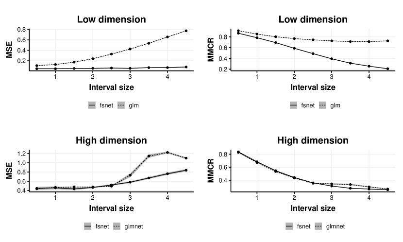
Figure 1: Sum of squared estimation errors and mean misclassification rates for the proposed method (fsnet), generalized linear models (glm), and lasso regression (glmnet). The shaded confidence bands are $\pm 1.96$ times the Monte Carlo standard errors.

6 Data examples

6.1 Lipoprotein data

Lipoprotein(a) [Lp(a)] is a risk factor for cardiovascular complications (see for example Littmann et al., (2019) or Littmann et al., (2022)). Hence, it is of interest to model the distribution of Lp(a) in different populations and to investigate the effects of covariates. One challenge is that Lp(a) has a lower limit of detection of 10 nanomoles per liter (nmol / L), leading to censoring from below. Additionally, in practice it Lp(a) is often categorized, into classes, such as those defined by deciles. We consider a regression model for Lp(a) in nmol / L in intervals $[0,10],(10,20],\dots,(110,120],(120,\infty)$. The data are a subset of those used by Littmann et al., (2019), except they use different classes, $[0,10],(10,30],(30,120],(120,\infty)$. There are $n=1837$ observations and four covariates: sex, age, smoking status (never-smoker, ex-smoker, or smoker), and hemoglobin A1c (HbA1c) measurements categorized into three levels (low, average, high) corresponding to good, average, and poor metabolic control.

We first fit a model for Lp(a) without predictors. One possibility is to fit the cumulative probability model in Example 1. As argued there, this is equivalent to fitting a general categorical model with $12$ parameters, the number of categories minus one. For concreteness, take $R$ to be the standard normal cumulative distribution function and denote the maximum likelihood estimate by $\widehat{\bm{\theta}}^{c}$. This estimate ensures $R(\widehat{\theta}^{c}_{j})=n^{-1}\sum_{i=1}^{n}Y_{i}\mathbb{I}(Y_{i}\leq 10j),j\in\{1,\dots,12\}$, where $\mathbb{I}(\cdot)$ is an indicator function. That is, the estimated category probabilities equal the sample proportions.

Another possibility is to assume the Lp(a) measurements come from a censored regression model such as in Example 2 with an intercept only. This can be particularly useful when interest is in inference on the unobservable continuous Lp(a). Because the model for the unobservable continuous Lp(a) is the same regardless of the censoring, this model facilitates pooling data from studies with different censoring. Since Lp(a) must be positive, we consider the model which assumes the continuous Lp(a), $Y_{i}^{*}$, satisfies

$$\log(Y_{i}^{*})=\beta+\sigma W_{i},$$

where $W_{i}\sim\mathcal{N}(0,1)$. Our response $Y_{i}$ is the interval containing $Y_{i}^{*}$. Fitting this model we get the maximum likelihood estimates $\hat{\beta}=3.02$ and $\hat{\sigma}=1.76$. These can be interpreted as usual in the latent regression, or one can focus on the estimated mass function for $Y_{i}$ given in Figure 2. Notably, the estimated probabilities are reasonably close to the sample proportions, or equivalently, the estimates from the cumulative probability model.

Figure 2: Estimated probability mass function for censored Lp(a)

The maximized likelihood for the latent regression model will always be lower than that of the cumulative probability model since the latter is equivalent to a general categorical model (Example 1). However, the former has fewer parameters and so may still be preferable. For example, computing the BIC for both models shows the smaller is preferable with a BIC of 7432 compared with 7480. We also considered letting $W_{i}$ have an extreme-value distribution, but that gave a BIC of 7481.

To investigate the effect of covariates, we continue with a latent regression model: $\log(Y_{i}^{*})=\bm{x}_{i}^{\mathsf{T}}\bm{\beta}+\sigma W_{i}$, $W_{i}\sim\mathcal{N}(0,1)$. Following Littmann et al., (2019), we consider the effect of age on Lp(a), and whether there are interactions between age and the other covariates. Considering the interactions first, we compare two models using a likelihood ratio test, a smaller one where

$$\bm{x}_{i}=[1,\mathtt{age}_{i},\mathtt{male}_{i},\mathtt{never\_smoker}_{i},\mathtt{smoker}_{i},\mathtt{average\_hba1c}_{i},\mathtt{high\_hb1ac}_{i}]^{\mathsf{T}},$$

and a larger one where $\bm{x}_{i}$ also includes age interacted with all the other predictors. The likelihood ratio test with 5 degrees of freedom gave a $p$-value of 0.19, indicating the interactions are not important.

Coefficient estimates and standard errors based on the observed information for the smaller model are in Table 1. The reported $p$-values are for Wald-type tests for whether a regression coefficient is zero and whether the scale parameter $\sigma=1$. Any $p$-value less than $10^{-4}$ is reported as $0$. In summary, there is evidence Lp(a) increases with age and is associated with poor metabolic control.

	Scale	Int.	Age	Male	Nev. Smoker	Smoker	Med. HbA1c	High HbA1c
Est.	1.74	2.6	0.011	-0.13	-0.20	-0.41	0.16	0.36
S.E.	0.046	0.21	0.0028	0.088	0.12	0.16	0.11	0.13
$p$-value	$0$	$0$	$0$	0.13	0.082	0.010	0.14	0.0067

Table 1: Regression for censored Lp(a)

6.2 Breast cancer data

We use data from the Netherlands Cancer Institute on $n=144$ lymph node positive women (van de Vijver et al.,, 2002). Following Tutz and Schmid, (2016, Examples 7.1 and 7.2), we model the time to development of distant metastases or death, in three-month intervals up to 15 months. For each patient the data include a follow-up time and an event indicator. The observable intervals are $[0,3),\dots,[12,15)$, or one of those intervals with the upper endpoint replaced by $\infty$ if the event (death or distant metastases) was not observed.

The data also include five clinical predictor variables (diameter of tumor $>$ 2 cm or not, number of affected lymph nodes $\leq$ 3 or not, estrogen receptor status positive or negative, tumor grade in three levels, and age) and gene expression measurements for 70 genes. We first consider a model using the clinical variables only, and then investigate whether the gene expression data can be used to improve out-of-sample predictions.

Suppose, as in Example 3, the continuous, unobservable time-to-event $T_{i}$ has cumulative distribution function $F(t_{i};\bm{x}_{i},{\bm{\beta}},{\bm{\gamma}})=1-\exp[-\exp\{\mathtt{sp}(\log t_{i};{\bm{\gamma}})-{\bm{\beta}}^{\mathsf{T}}\bm{x}_{i}\}],$ where $\mathtt{sp}$ is a spline function. Specifically, we pick the I-splines discussed by Ramsay, (1988) with no knots and three degrees of freedom, implemented in the R package splines2 (Wang and Yan,, 2021). These splines are monotone if the elements of ${\bm{\gamma}}$ are non-negative, which we therefore enforce when fitting. Exponential and Weibull interval-censored models are special cases corresponding to, respectively, $\mathtt{sp}(\log t;\gamma)=\log t$ and $\mathtt{sp}(\log t;\gamma)=\gamma\log t$. The three models are nested and upon fitting and comparing them using likelihood ratio tests, we got the $p$-value 0.83 when testing the flexible I-splines against Weibull, 0.88 for Weibull against exponential, and 0.53 for the flexible I-splines against the exponential.

Figure 3 shows estimated survival probabilities for the flexible I-splines and exponential models. In the figure, the clinical predictors are held at their median values. The first plot shows a marked difference in estimated survival probabilities in the right tail for the unobservable, continuous survival times. However, for the observable data only the probabilities at months $3,6,\dots,15$ matter. Indeed, any two survival functions that agree at those points give the same distribution for the observed data. The second plot in Figure 3 shows the two models give similar survival probabilities at the relevant points, consistent with the large $p$-values obtained when comparing the different models. We focus on the exponential model for the remainder of the section.

Figure 3: Estimated survival probabilities for breast cancer data

Table 2 shows results from fitting the exponential model. The reported standard errors are square roots of diagonal entries of the inverse of the observed Fisher information matrix. The $p$-values are Wald-type and are for the null hypotheses that coefficients are zero. The number of affected lymph nodes appears to be an important predictor, and there is some evidence the tumor grade may be important.

	Intercept	Diam. $>$ 2	Nodes $\leq 3$	E.R. Pos.	Grade.L	Grade.Q	Age
Est.	0.00072	-0.30	0.77	0.58	0.55	0.26	0.051
S.E.	1.1	0.33	0.34	0.36	0.33	0.26	0.028
$p$-value	1.0	0.35	0.022	0.11	0.098	0.33	0.068

Table 2: Regression for three-month time-to-event

We next consider prediction using the gene expression measurements. Let $\bm{h}_{i}\in\mathbb{R}^{70}$ be a vector of gene expression measurements, standardized to have sample mean zero and unit sample variance. We are interested in whether the $\bm{h}_{i}$ can be used to improve the predictive performance of our method, and if so, selecting genes useful for that purpose. To investigate we randomly split the data into a test set of $144/3=48$ observations and a training set of $96$ observations. We consider the exponential model with predictor vector $[\bm{x}_{i}^{\mathsf{T}},\bm{h}_{i}^{\mathsf{T}}]^{\mathsf{T}}\in\mathbb{R}^{77}$ and coefficient vector ${\bm{\theta}}=[{\bm{\beta}}^{\mathsf{T}},\bm{\alpha}^{\mathsf{T}}]^{\mathsf{T}}\in\mathbb{R}^{77}$, so $\bm{\alpha}\in\mathbb{R}^{70}$ is the coefficient vector for the gene expressions. Consider the estimators $\widehat{{\bm{\theta}}}=(\widehat{{\bm{\beta}}},\widehat{\bm{\alpha}})\in\operatorname*{arg\,min}_{{\bm{\theta}}\in\mathbb{R}^{77}}\{G_{n_{t}}({\bm{\theta}})+\lambda\|\bm{\alpha}\|_{1}\}$ and $\widetilde{{\bm{\beta}}}\in\operatorname*{arg\,min}_{{\bm{\beta}}\in\mathbb{R}^{7}}G_{n_{t}}([{\bm{\beta}}^{\mathsf{T}},0]^{\mathsf{T}}),$ where $n_{t}=96$ is the number of observations in the training set. The former estimator penalizes the coefficients for the gene expression measurements while the latter assumes those coefficients are zero. Thus, $\widetilde{{\bm{\beta}}}$ is the maximum likelihood estimator in the exponential model without gene expressions, using the training set only.

The penalty parameter $\lambda$ was selected from the set $\{\exp(-10),\dots,\exp(0)\}$ by five-fold cross-validation on the training set. This gave $\lambda=\exp(-5)\approx 0.0067$, which attained an average misclassification rate of 0.29 over the five folds. Predictions on the test-set with the selected $\lambda$ gave an out-of-sample misclassification rate of 0.31. By comparison, using the clinical predictors only, that is, the predictions $\exp(\bm{x}_{i}^{\mathsf{T}}\widetilde{{\bm{\beta}}})$, gave a misclassification rate of 0.44. We conclude the gene expression measurements can improve prediction, agreeing with the findings of Tutz and Schmid, (2016).

With $\lambda=\exp(-5)$, 32 of the 70 elements of $\widehat{\bm{\alpha}}$ were zero. The Supporting Information contains a trace plot showing how the number of non-zero coefficients and their sizes vary with $\lambda$.

7 Conclusion

The fact that observed data have finite support ought to be considered before using models for continuous random variables, which in general leads to misspecification bias. Roughly speaking, the smaller the cardinality of the support and the variance of maximum likelihood estimators are, the more pronounced the misspecification bias is. Even in settings where the bias is small, however, the effects of using a misspecified likelihood can be difficult to assess, leading to unreliable inference. With the methods proposed here practitioners have access to fast and reliable likelihood-based inference, in both low- ($n<d$) and high-dimensional ($d>n$) regression problems. There is a wide range of possible applications, including but not limited to survival analysis in discrete time, ordinal regression, and interval-censored linear regression. Moreover, while the presented theory made repeated use of the concavity of the log-likelihood, (1) gives a valid model even if $r$ is not log-concave. Thus, the modeling framework can be extended to many settings not discussed in the present paper.

Possible directions for future research include the development of theory for the interplay between the severity of censoring and the properties of maximum likelihood estimators. For example, it may be informative to consider asymptotics where the length of the censoring intervals is allowed to change with the sample size and the number of parameters. Additionally, several special cases of the models considered herein are also of significant interest in their own right, and may hence merit further study. As noted in Section 3, more informative high-dimensional convergence bounds can likely be obtained for special cases. It may also be worthwhile to explore settings with dependent data. In the present setting, some types of dependent responses may be analyzed by joining their supports. For example, two dependent binary responses can be recoded as one response with four possible outcomes. The present setting could also in principle be extended to include random effects in the linear predictors, but the theory and implementation would require substantial work.

References

- Agresti, (2019) Agresti, A. (2019). An Introduction to Categorical Data Analysis. Wiley Series in Probability and Statistics. John Wiley & Sons, Hoboken, NJ, third edition edition.
- Beck and Teboulle, (2009) Beck, A. and Teboulle, M. (2009). A fast iterative shrinkage-thresholding algorithm for linear inverse problems. SIAM Journal on Imaging Sciences, 2(1):183–202.
- Burridge, (1981) Burridge, J. (1981). A note on maximum likelihood estimation for regression models using grouped data. Journal of the Royal Statistical Society. Series B (Methodological), 43(1):41–45.
- Burridge, (1982) Burridge, J. (1982). Some unimodality properties of likelihoods derived from grouped data. Biometrika, 69(1):145–151.
- Byrd et al., (2016) Byrd, R. H., Nocedal, J., and Oztoprak, F. (2016). An inexact successive quadratic approximation method for L-1 regularized optimization. Mathematical Programming, 157(2):375–396.
- Couso et al., (2017) Couso, I., Dubois, D., and Hüllermeier, E. (2017). Maximum Likelihood Estimation and Coarse Data. In Moral, S., Pivert, O., Sánchez, D., and Marín, N., editors, Scalable Uncertainty Management, Lecture Notes in Computer Science, pages 3–16, Cham. Springer International Publishing.
- Finkelstein, (1986) Finkelstein, D. M. (1986). A proportional hazards model for interval-censored failure time data. Biometrics, 42(4):845.
- Friedman et al., (2010) Friedman, J. H., Hastie, T., and Tibshirani, R. (2010). Regularization paths for generalized linear models via coordinate descent. Journal of Statistical Software, 33(1):1–22.
- Gentleman and Geyer, (1994) Gentleman, R. and Geyer, C. J. (1994). Maximum likelihood for interval censored data: Consistency and computation. Biometrika, 81(3):618–623.
- Guillaume et al., (2017) Guillaume, R., Couso, I., and Dubois, D. (2017). Maximum likelihood with coarse data based on robust optimisation. In Proceedings of the Tenth International Symposium on Imprecise Probability: Theories and Applications, pages 169–180.
- Heitjan, (1989) Heitjan, D. F. (1989). Inference from grouped continuous data: A review. Statistical Science, 4(2):164–179.
- Hjort and Pollard, (2011) Hjort, N. L. and Pollard, D. (2011). Asymptotics for minimisers of convex processes.
- Huang, (1996) Huang, J. (1996). Efficient estimation for the proportional hazards model with interval censoring. Annals of Statistics, 24(2):540–568.
- Kowal and Canale, (2020) Kowal, D. R. and Canale, A. (2020). Simultaneous transformation and rounding (STAR) models for integer-valued data. Electronic Journal of Statistics, 14(1):1744–1772.
- Lee et al., (2006) Lee, S.-I., Lee, H., Abbeel, P., and Ng, A. Y. (2006). Efficient L1 regularized logistic regression. In Aaai, volume 6, pages 401–408.
- Littmann et al., (2022) Littmann, K., Hagström, E., Häbel, H., Bottai, M., Eriksson, M., Parini, P., and Brinck, J. (2022). Plasma lipoprotein(a) measured in the routine clinical care is associated to atherosclerotic cardiovascular disease during a 14-year follow-up. European Journal of Preventive Cardiology, 28(18):2038–2047.
- Littmann et al., (2019) Littmann, K., Wodaje, T., Alvarsson, M., Bottai, M., Eriksson, M., Parini, P., and Brinck, J. (2019). The Association of Lipoprotein(a) Plasma Levels With Prevalence of Cardiovascular Disease and Metabolic Control Status in Patients With Type 1 Diabetes. Diabetes Care, 43(8):1851–1858.
- McGough et al., (2021) McGough, S. F., Incerti, D., Lyalina, S., Copping, R., Narasimhan, B., and Tibshirani, R. (2021). Penalized regression for left-truncated and right-censored survival data. Statistics in Medicine, 40(25):5487–5500.
- Milzarek and Ulbrich, (2014) Milzarek, A. and Ulbrich, M. (2014). A semismooth Newton method with multidimensional filter globalization for L1-Optimization. SIAM Journal on Optimization, 24:298–333.
- Negahban et al., (2009) Negahban, S., Yu, B., Wainwright, M. J., and Ravikumar, P. (2009). A unified framework for high-dimensional analysis of M-estimators with decomposable regularizers. Advances in neural information processing systems, 22.
- Negahban et al., (2012) Negahban, S. N., Ravikumar, P., Wainwright, M. J., and Yu, B. (2012). A unified framework for high-dimensional analysis of M-estimators with decomposable regularizers. Statistical Science, 27(4).
- Prékopa, (1973) Prékopa, A. (1973). On logarithmic concave measures and functions. Acta Scientiarum Mathematicarum, 34:335–343.
- Ramsay, (1988) Ramsay, J. O. (1988). Monotone regression splines in action. Statistical Science, 3(4):425–441.