Multi-Objective reward generalization: Improving performance of Deep Reinforcement Learning for applications in single-asset trading

Abstract.

We investigate the potential of Multi-Objective, Deep Reinforcement Learning for stock and cryptocurrency single-asset trading: in particular, we consider a Multi-Objective algorithm which generalizes the reward functions and discount factor (i.e., these components are not specified a priori, but incorporated in the learning process).

Firstly, using several important assets (cryptocurrency pairs BTCUSD, ETHUSDT, XRPUSDT, and stock indexes AAPL, SPY, NIFTY50), we verify the reward generalization property of the proposed Multi-Objective algorithm, and provide preliminary statistical evidence showing increased predictive stability over the corresponding Single-Objective strategy. Secondly, we show that the Multi-Objective algorithm has a clear edge over the corresponding Single-Objective strategy when the reward mechanism is sparse (i.e., when non-null feedback is infrequent over time). Finally, we discuss the generalization properties with respect to the discount factor.

The entirety of our code is provided in open source format.

1. Introduction

The algorithm developed by Fontaine and Friedman (Friedman and Fontaine, 2018) (see also (Castelletti et al., 2012; Ernst et al., 2005)) is a specific declination of Multi-Objective Reinforcement Learning (RL): while we postpone rigorous details to the next sections below, we can – for now – informally describe this as a RL declination which allows to simultaneously train all possible strategies associated with exploring a dynamic environment. Specifically, each strategy is identified by the reward mechanism associated with a given linear combination of multiple, pre-specified (and possibly conflicting) objective functions. This simultaneous learning process over all possible strategies, which gives the user the freedom to specify the combination of the objective functions after the training has been completed, makes the RL declination in (Friedman and Fontaine, 2018) highly interpretable and versatile.

While the techniques in (Friedman and Fontaine, 2018) have so far been successfully applied in several fields, applications of such a methodology for financial purposes are – to the best of our knowledge – still lacking. In this paper, we show the potential entailed by using such a Multi-Objective Reinforcement Learning algorithm – along with meaningful variations of the same – in the context of single-asset stock and cryptocurrency applications. We validate our results by deploying the algorithm on several important assets, namely: cryptocurrency pairs BTCUSD, ETHUSDT, XRPUSDT, and stock indexes AAPL, SPY, NIFTY50. Additionally, we discuss the generalization with respect to the discount factor parameter.

We now give more precise details for the terminology so far informally introduced.

1.1. Reinforcement Learning: basics

Reinforcement Learning (RL) is a subfield of Machine Learning specifically designed to handle learning processes for problems which involve a dynamic interaction with a given underlying environment. RL techniques have initially been deployed – among many – in the field of gaming (Mnih et al., 2013), robotics (Kober et al., 2013), personalized recommendations (Zheng et al., 2018), and resource management (Mao et al., 2016).

1.1.1. Single-Objective RL

A RL algorithm learns to use the set of observable state variables $\boldsymbol{s}$ (describing the current state of the environment) to take the most appropriate admissible action $a$. For a general RL algorithm, the state variables and action $(\boldsymbol{s},a)$ and the environment’s intrinsic stochasticity determine the next state of the environment that the algorithm will visit: the exact way in which this task is accomplished varies depending on the specific algorithm. For example, the RL algorithms of so-called critic–only form (see (Sutton and Barto, 2018)) aim to maximize a single, cumulative reward (accounting for all actions taken in a given episode), which is in turn based on a pre-specified state–action reward function $r$ (assigning a numerical reward $r(\boldsymbol{s},a)$ to every pair $(\boldsymbol{s},a)$ of given state and action undertaken). The algorithm uses several episodes (each accounting for an exploration of the environment which ends when a pre-specified end-state is reached) to train its decision-making capabilities (by progressively updating the so-called $Q$-values (Sutton and Barto, 2018) throughout the episodes).

1.1.2. Multi-Objective RL

Multi-Objective RL is a declination of RL devoted to learning in environments with vector-valued – rather than scalar – rewards. Such a setting – which allows to cover realistic scenarios in which conflicting metrics are present – has been gaining a lot of traction lately. Two rather comprehensive surveys on the topic that we are aware of are (Rădulescu et al., 2020; Roijers et al., 2013). With methodologies including – among many others – Pareto front-type analysis (Zitzler et al., 2008; Reymond and Nowé, 2019), dynamic multi-criteria average reward reinforcement learning (Natarajan and Tadepalli, 2005), convex hull value iteration (Barrett and Narayanan, 2008), Hindsight Experience Replay techniques (Andrychowicz et al., 2017), dynamic weights computation (Abels et al., 2019), tunable dynamics in agent-based simulation (Källström and Heintz, 2019), Deep Optimistic Linear Support Learning (DOL) for high-dimensional decision problems (Mossalam et al., 2016), Deep Q-networks techniques (Nguyen et al., 2020; Tajmajer, 2017, 2018), and collaborative agents systems (Dusparic and Cahill, 2009), it is safe to say that the Multi-Objective RL paradigm is well-established in several non-finance related applications.

1.2. Reinforcement Learning in finance

The problems we are interested in are related to using RL for profitable, risk-reduced trading of financial tools based on historical data. These problems are usually quite challenging to tackle using AI, and this is mostly due to three factors: i) high data noisiness of financial environment; ii) subjective definition of the financial environment, and iii) non reproducibility of the financial environment (only a single copy of any given time series is available for training).

Despite these difficulties, a prolific literature is available: the summary report (Fischer, 2018) provides an exhaustive overview of the main works associated with the three most commonly used RL paradigms (i.e., critic-, actor-, and actor/critic- based techniques) for financial applications. Among critic-based works, we find superiority of RL over standard supervised learning approaches (Neuneier, 1995), performance improvement assessments with respect to varying reward functions and hyperparameters (Corazza and Bertoluzzo, 2014), Deep Q-learning (DQL) extensions to trading systems (Jin and El-Saawy, 2016), evolutionary reinforcement learning in the form of genetic algorithms (Dempster et al., 2001; Gu et al., 2011), identification of seasonal effects (Tan et al., 2011; Eilers et al., 2014), high-frequency analysis (Sherstov and Stone, 2004), trade execution optimization (Nevmyvaka et al., 2006), dynamical allocation of high-dimensional assets, (Kaur, 2017; Jangmin et al., 2006), and hedging basis risk assessment (Watts, 2015). For actor-based methods, we mention recurrent reinforcement learning baselines (Moody et al., 1998; Gold, 2003), multi-layered risk management systems (Dempster and Leemans, 2006), and high-level feature extraction (Deng et al., 2016; Jiang et al., 2017). Finally, we quote (Li et al., 2007; Bekiros, 2010; Chan and Shelton, 2001) as representatives of the actor/critic-based category.

1.2.1. Multi-Objective RL in finance

While the Multi-Objective RL paradigm is well-established in several non-finance related applications (see discussion of Subsection 1.1.2), it appears to still be relatively under-explored in the context of financial markets.

In this context, the most commonly taken approach to Multi-Objective RL is to indirectly embed the desired multi-reward effects in parts of the model other than the reward mechanism itself (e.g., collaborating market agents (Lee and Jangmin, 2002; Lee et al., 2007, 2002)). Another approach is to consider an intrinsic Multi-Objective approach, but without generalization (i.e., the reward weights are set a priori, and are not part of the learning process). This is the case for the two reference works (Bisht and Kumar, 2020; Si et al., 2017), which we summarize in Section 3.

2. Our contribution

We use a generalized, intrinsically Multi-Objective RL strategy for stock and cryptocurrency trading. We implement this by considering extensions of Multi-Objective Deep Q-Learning RL algorithm with experience replay and target network stabilization given in (Friedman and Fontaine, 2018), and deploying it on several important cryptocurrency pairs and stock indexes.

2.1. Main Results

Our main findings – which we have validated on several datasets including AAPL, SPY, ETHUSDT, XRPUSDT, BTCUSD, NIFTY50– are summarized as follows.

:

$\bullet$ Generalization. We show that our Multi-Objective RL algorithm generalizes well between four reward mechanisms (last logarithmic return, Sharpe ratio, average logarithmic return, and a sparse reward triggered by closing positions).

:

$\bullet$ Stability on prediction. We use two metrics (Sharpe Ratio and cumulative profits) to show that the prediction of our Multi-Objective algorithm is more stable than the corresponding Single-Objective strategy’s.

:

$\bullet$ Advantage for sparse rewards. We show that the results of the Multi-Objective algorithm are significantly better than those of the corresponding Single-Objective algorithm in the case of sparse rewards.

:

$\bullet$ Discount factor generalization. We provide partial evidence of generalization of the discount factor: this parameter is the RL time-regularization parameter in (1) below.

:

$\bullet$ Impact of fees. As per the nature of the current underlying RL algorithm (for both Multi-Objective and Single-Objective), trading fees diminish every performance to zero. This behavior is to be expected, see mitigating circumstances described in Subsection 2.3.2 and Subsection 2.3.3 below.

2.2. Validation of results

In order to show the robustness of our analysis, we adhere to the following general strategy.

:

$\bullet$ Large number of datasets. We run our experiments on a large group of single-asset financial time series: in particular, these include cryptocurrency pairs (BTCUSD, ETHUSDT, XRPUSDT) and stock indexes (AAPL, SPY, NIFTY50).

:

$\bullet$ Different initializations. In order to detach the impact of the chosen neural network’s random initialization from the actual results, we perform several independent trainings for each given dataset we run our algorithm on. This is used to assess the distribution of gains for our algorithm.

:

$\bullet$ Cross-validation. We further confirm the effectiveness of our method using a plain hold-out method and walk-forward cross-validation with anchoring (i.e., where the training set starting date is the same for all folds).

2.3. Practical implications and considerations

We highlight some of the most important aspects of our approach from an applied perspective.

2.3.1. Simplicity and interpretability

We deploy an intuitive and interpretable Multi-Objective RL algorithm in order to account for several – well established – reward mechanisms in single-asset trading. We view this methodology as having a strong applied connotation, and being complementary to other existing Multi-Objective strategies for financial problems (Lee and Jangmin, 2002; Bisht and Kumar, 2020; Si et al., 2017).

2.3.2. Zero-fee setting

Although our analysis is conducted in a zero-fee market context, such a context nonetheless applies to many meaningful markets. For retail traders zero-fee spot trading is possible on multiple markets, for example BTCUSDspot on the cryptocurrency exchange Binance. For institutional traders even more opportunities exist, since they can often operate in low to zero or fixed fee market contexts by directly working together with market makers.

2.3.3. Underlying RL algorithm

Our main focus is always to compare our generalized Multi-Objective RL methodology to a corresponding Single-Objective strategy: said differently, we do not so much dwell on increasing the performance of the underlying RL strategy (in fact, we choose a rather simple critic-based RL declination), as we do on evaluating the difference of the Single-/Multi-Objective methods for the same underlying RL method.

Remark 1.

The adaptation of this methodology with more sophisticated underlying RL methods is deferred to future works.

2.4. Structure of the paper

We summarize the main contributions of the related works (Bisht and Kumar, 2020; Si et al., 2017) in Section 3. We provide the abstract setup of our proposed Algorithm in Section 4, and fill in the necessary quantitative details in Section 5. After spelling out the main technical features related to our code (see Section 6), we discuss our main results in Section 7. Conclusions (respectively, future outlook) are given in Section 8 (respectively, Section 9). The precise details concerning our chosen underlying RL algorithm are provided in the Appendix A.

3. Related work

The works (Bisht and Kumar, 2020; Si et al., 2017) use multi-reward scalarization to improve on the following, well-established benchmark strategies in the context of price prediction in single-asset trading: i) an actor-only, RL algorithm with total portfolio value as single reward, and; ii) a standard Buy-and-Hold strategy. More specifically, the authors take as rewards the average and standard deviations from the classical definition of the Sharpe ratio, and combine them with pre-defined weights to favor risk-adjustment. In another variation, the resulting scalarized metric is modified to further penalize negative volatility.

The authors use a two-block LSTM neural network to directly map the last previously taken action (Buy/Sell/Hold) and the available state variables to the next action. The first LSTM block is used for high-level feature extraction, and the other one for reward-oriented decision-making. From the experimental results the authors conclude superiority of their method over to the two benchmarks in terms of cumulative profit and algorithm convergence, although an analysis of statistical significance is not provided.

While the scalarization approach is effective, it nonetheless has the downside of having to a priori specify the balance of the individual rewards (via their weights). This introduces a human factor into the balancing of rewards, and also restricts the scope of the learning process. Driven by this, we choose not to scalarize the reward metrics, so that the weights can be included in the learning process. To the very best of our knowledge, ours is the first application of Multi-Reward RL in the sense of (Friedman and Fontaine, 2018) to financial data.

4. Abstract definition of the model

We consider variations of the Deep-Q-Learning algorithm with Hindsight Experience Replay and target network stabilization (Sutton and Barto, 2018) (DQN-HER) for both standard Single-Reward or Multi-Reward structure (in the sense of (Friedman and Fontaine, 2018)), and apply them to single asset trading problems.

4.1. The classical abstract setup

The basic structure of (DQN-HER) is concerned with maximizing cumulative rewards of the type

(1) $$R_{t}=\sum_{i=t}^{T}{\gamma^{i}r_{i}},$$

where $\gamma\in(0,1)$ is the so-called discount factor. The discount factor determines the time preference of the agent and regularizes the reward as $T\rightarrow\infty$. A small discount factor makes short-term rewards more favorable. The algorithm fits a neural network taking the current state $\boldsymbol{s}_{t}$ as input and giving an estimate of the maximum cumulative reward of type (1) achievable by subsequently taking each permitted action $a_{t}$. The learning process is linked to the Bellman’s equation update

$$[Q(\boldsymbol{s}_{t})]_{a_{t}} =(1-\alpha)[Q(\boldsymbol{s}_{t})]_{a_{t}}$$

(2) $$\quad+\alpha\left(r(\boldsymbol{s}_{t},a_{t})+\gamma\max_{a_{t+1}}{[Q(\boldsymbol{s}_{t+1})]_{a_{t+1}}}\right)$$

for a given learning rate $\alpha\in(0,1)$, and where $r(\boldsymbol{s_{t}},a_{t})$ is the reward for taking action $a_{t}$ in state $\boldsymbol{s}_{t}$.

4.1.1. Multi-Reward adaptation in the sense of (Friedman and Fontaine, 2018)

With respect to the previous case, the neural network’s input is augmented by a reward weight vector $\boldsymbol{w}$, which is used to compute the total reward $\boldsymbol{w}\cdot\boldsymbol{r}(\boldsymbol{s}_{t},a_{t})$ (here $\boldsymbol{r}$ is the vector of rewards, and $\cdot$ denotes the standard scalar product). The Single-Reward case can be seen as a declination of the Multi-Reward case with constant suitable one-hot encoding vectors $\boldsymbol{w}$. The (DQN-HER) algorithm is summarized in Algorithm 1 for the reader’s convenience.

4.2. Our abstract setup

The methodology we adopt in this paper is summarized in Algorithm 2, and stems from the underlying basic Algorithm 1. For the sake of clarity, Algorithm 2 highlights only the changes between the two algorithms. These modifications are related to:

:

i) an option for ‘random access point’: subject to specification by the user, each training episode may use a subset of the full price history of the training set, where the starting point is randomly sampled and the length is fixed;

:

ii) the generalization of the discount factor $\gamma$ as suggested in (Friedman and Fontaine, 2018): this means that the neural network’s input also comprised the discount factor $\gamma$ (i.e., input is augmented from $(\boldsymbol{s},\boldsymbol{w})$ to $(\boldsymbol{s},\boldsymbol{w},\gamma)$);

:

iii) the specific choice of normalization spelled out in Subsection 4.2.1 below.

4.2.1. Choice of Normalization

We choose to indirectly normalize the neural network’s output variables (i.e., the approximate $Q$-values) by rescaling the rewards in the Bellman’s update (4.1). More precisely, whenever a mini-batch

$$\{(\boldsymbol{s}_{i},\gamma_{i},\boldsymbol{w}_{i},\boldsymbol{w}_{i}\cdot\boldsymbol{r}(\boldsymbol{s}_{i},a_{i}),a_{i},\boldsymbol{s}_{i,new})\}_{i\in B},\qquad B\subset\{1,\dots,\#\mathcal{R}\}$$

is randomly sampled from the replay $\mathcal{R}$ (see Algorithm 2, line 22), the rescaled vectors

(3) $$\displaystyle\tilde{\boldsymbol{r}}(\boldsymbol{s}_{i},a_{i}) =\frac{\Sigma^{-1/2}\boldsymbol{r}(\boldsymbol{s}_{i},a_{i})}{\|\boldsymbol{w}_{i}\|_{2}},\qquad i\in B$$

and associated scalar rewards $\{\boldsymbol{w}_{i}\cdot\tilde{\boldsymbol{r}}(\boldsymbol{s}_{i},a_{i})\}_{i\in B}$ are fed to the training in place of the original sets $\{\boldsymbol{r}(\boldsymbol{s}_{i},a_{i})\}_{i\in B}$ and $\{\boldsymbol{w}_{i}\cdot\boldsymbol{r}(\boldsymbol{s}_{i},a_{i})\}_{i\in B}$. Here, the matrix $\Sigma$ denotes the approximate covariance matrix computed using the reward vectors from the entire replay, namely

$$\Sigma=\mbox{Cov}\left(\{\boldsymbol{r}(\boldsymbol{s}_{i},a_{i})\}_{i\in\{1,\dots,\#\mathcal{R}\}}\right).$$

With this choice, the overall scalar rewards $\{\boldsymbol{w}_{i}\cdot\tilde{\boldsymbol{r}}(\boldsymbol{s}_{i},a_{i})\}_{i\in B}$ are normalized, in the sense that

(4) $$\mbox{Cov}\left(\{\boldsymbol{w}_{i}\cdot\tilde{\boldsymbol{r}}(\boldsymbol{s}_{i},a_{i})\}_{i\in B}\right)=1.$$

4.2.2. Length of the Experience Replay

We exclusively use a same-age type experience replay: more precisely, the experience replay’s oldest element (measured in number of network updates following its creation) is the same for both Single– and Multi–Reward case. In the Multi-Reward case, where extra – not visited – experiences are thrown into the replay (Algorithm 1-line 19), this results in a longer replay.

5. Specific details of our model

After having laid out the general structure of our RL setup (see Algorithm 2), we give precise substance to all quantities involved.

5.1. State variables $\boldsymbol{s}_{t}$

We define the state variables $\boldsymbol{s}_{t}$ as the vector comprising both the current position in the market (which we name $p_{t}$, and whose precise details are given in Subsection 5.2 below) and a fixed lookback of length $\ell$ over the most recent log returns of close prices $\{z_{t}\}_{t}$: more explicitly, we set

(5) $$\boldsymbol{s}_{t}:=\left(\left\{\ln z_{s}-\ln z_{s-1}\right\}_{s=t-(\ell-1)}^{t},\,p_{t}\right)\in\mathbb{R}^{\ell}\times\mathbb{R}.$$

5.2. Admissible Actions and Positions

As far as actions are concerned, we analyze two scenarios:

• Long Positions only (LP): The agent is only allowed to perform two actions (Buy/Hold), and consequently only switch between trading positions Long/Neutral.

• Long and Short Positions (L&SP): the agent is allowed to perform three actions (Buy/Sell/Hold), and consequently switch between trading positions Long/Short/Neutral.

5.3. Rewards and Profit

For a given single-asset dataset with close prices $\{z_{t}\}_{t}$, we define the logarithmic (portfolio) return at time $t$ as

(9) $$\ell r_{t}:=\left\{\begin{array}[]{rl}\ln z_{t}-\ln z_{t-1},&\mbox{ if in {\tt Long} at time }t-1,\\ -\left(\ln z_{t}-\ln z_{t-1}\right),&\mbox{ if in {\tt Short} at time }t-1,\\ 0,&\mbox{ if in {\tt Neutral} at time }t-1.\end{array}\right.$$

Let $L\in\mathbb{N}$ be fixed. We focus on three well-established rewards (at a reference given point in time $t$), namely:

:

i) the last logarithmic return (LR), which is exactly (9);

:

ii) the average logarithmic return (ALR), given by

$$\mbox{ALR}:=\mbox{mean}\left[\left\{\ell r_{s}\right\}_{s=t-(L-1)}^{t}\right];$$

:

ii) the non-annualized Sharpe Ratio (SR), given by

$$\mbox{SR}:=\frac{\mbox{mean}\left[\left\{\ell r_{s}\right\}_{s=t-(L-1)}^{t}\right]}{\mbox{std}\left[\left\{\ell r_{s}\right\}_{s=t-(L-1)}^{t}\right]},$$

as well as the sparse, less conventional reward:

:

iv) a ‘profit-only-when-(position)-closed’ (POWC) reward, defined as

$$\mbox{POWC}:=\left\{\begin{array}[]{rl}\ln z_{t}-\ln z_{t_{LT}},&\mbox{ if {\tt Long} closed at time }t-1,\\ -\left(\ln z_{t}-\ln z_{t_{LT}}\right),&\mbox{ if {\tt Short} closed at time }t-1,\\ 0,&\mbox{ otherwise},\end{array}\right.$$

where $t_{LT}$ is the time of last trade (i.e., last position change).

6. Experiments

We substantiate all necessary components involved in the simulations of our model (given in Algorithm 2).

6.1. Codebase

For the structure of our code, we took some inspiration from two open source repositories: the FOREX and stock environment at

https://github.com/AminHP/gym-anytrading

and the minimal Deep Q-Learning implementation at

https://github.com/mswang12/minDQN .

6.1.1. Open source directory and reproducibility

Our entire code is provided in open source format at

https://github.com/trality/fire .

In particular: the instructions for reproducibility are contained in the README.md file therein; we provide the entirety of the datasets considered in our experiments.

6.2. Datasets

We perform several runs of experiments on a variety of relevant single-asset datasets, both in cryptocurrency and stock trading.

In the interest of increasing the training capabilities of our experiments (see Subsection 7.4 below), we always include an evaluation set in addition to train and test sets. The percentages of the data associated with training/evaluation/test sets are roughly train:64%–eval:16%–test:20%. All datasets are of sufficient length as to provide a reasonable compromise between experiment running times, and significance of predictions.

6.2.1. Cryptocurrency pairs

We consider the following datasets: hourly-data points for the BTCUSD pair (August 2017–June 2020); hourly-data points for the ETHUSDT pair (August 2017–June 2020); hourly-data points for the XRPUSDT pair (May 2018–March 2021).

6.2.2. Stock indexes

We consider the indexes AAPL, SPY, NIFTY50. The date range for AAPL, SPY is January $2000$–September $2022$ (daily-data points), while for NIFTY50 is March $2020$–June $2020$ (minute-data points).

A snapshot example from the datasets BTCUSD and NIFTY50 is shown in Figure 1.

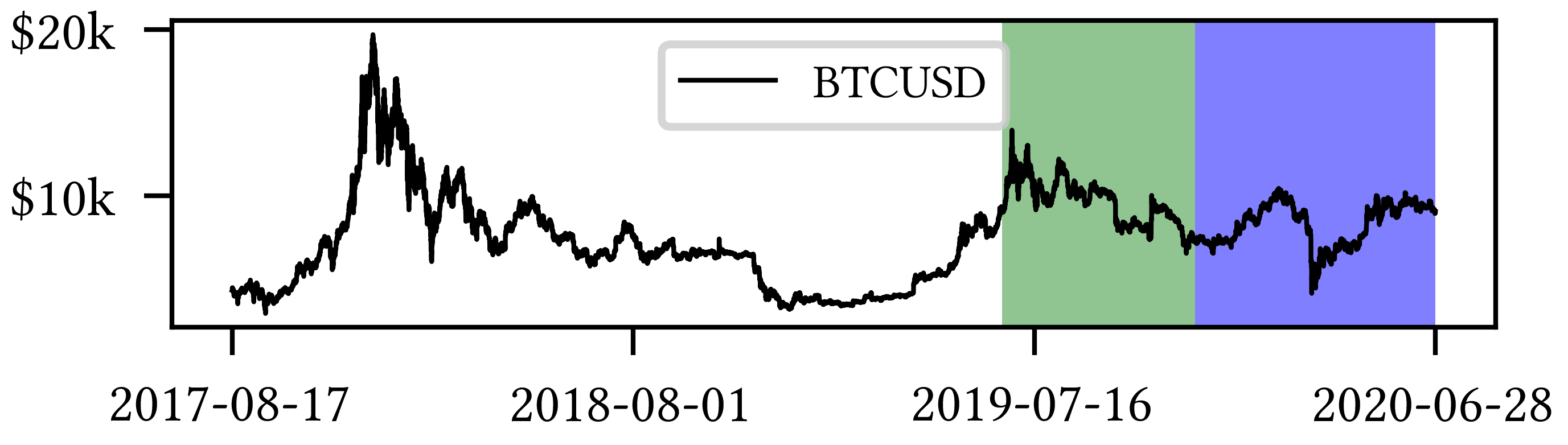
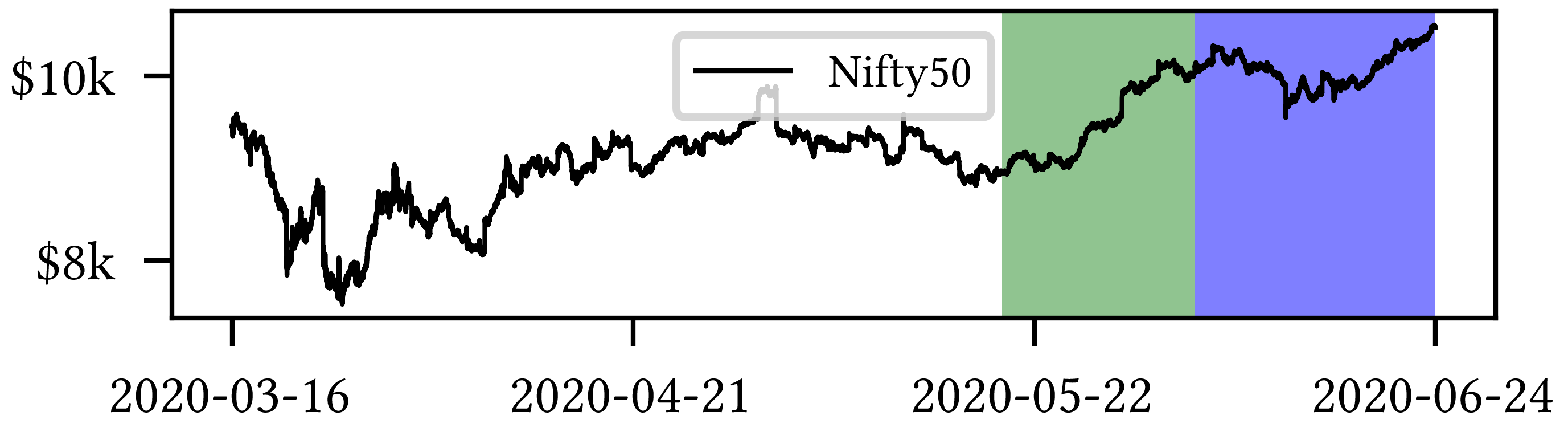
Figure 1. Close prices for train (white), evaluation (green), and test set (blue). Top (Bottom): BTCUSD (NIFTY50). We notice the mostly downward trend (respectively, strongly upward trend) on the BTCUSD (NIFTY50) evaluation set.

DataSetsCryptocurrency

6.3. Quantities of interest and benchmarks

All our considerations will be based on the following – quite standard – quantities:

• Total Reward: the cumulative reward over the considered portion of the dataset.

• Total Profit: the cumulative gain/loss obtained by buying or selling with all the available capital at every trade.

• Sharpe Ratio: the average return per step, divided by the standard deviation of all returns.

Crucially, results of Multi and Single-rewards simulations are compared against each other, as well as – individually – also against the Buy-and-Hold strategy.

6.4. Measures for code efficiency

6.4.1. Basic measures

The most important measures taken in this regard are as follows. Firstly, as we are primarily interested in assessing the potential superiority of a Multi-Reward approach over a Single-Reward one (see discussion in Subsection 2.3.3), we decide to stick to a simple Multi Layer Perceptron (MLP) Neural Network (Algorithm 1- line 2). Secondly, for the purpose of checking the performance in between training, we run the currently available model on full training and evaluation sets only for an evenly distributed subspace of episodes.

6.4.2. Option of random access point

If we choose the walk-forward cross-validation, the training in each episode is performed on a randomly selected, contiguous subset of the full training set with pre-specified length (this reduces the overall training cost).

6.4.3. Vectorized computation of $Q$-values

Except for the trading position $p_{t}$, the time evolution of the state variables vector given in (5) is otherwise entirely predictable (as prices $z_{t}$ obviously do not change in between training episodes). This implies that, given a predetermined set of $n$ actions, the algorithm can efficiently vectorize the evaluation of the neural network for each separate trading position, and then deploy the results to speedily compute the associated $n$ future steps. This method is feasible as the cardinality of admissible values of non-predictable state variables (i.e., the trading position) is low (three at most, in the L&SP case).

7. Results

The results arising from several Multi and Single-Reward experiments (using Algorithm 2) on several datasets (BTCUSD, ETHUSDT, XRPUSDT, AAPL, SPY, NIFTY50) give us four general indications, which we discuss below in detail in as many dedicated subsections. We support our analysis using different types of plots, namely:

:

i) distribution of performance (box-plots for various rewards over train/eval/test sets) obtained using several independent experiment realizations, see Figure 20 as an example;

:

ii) cumulative rewards on train/eval sets (as functions of epochs), see Figure 6 as an example, and;

:

iii) for each epoch, the Sharpe Ratio on eval set of the current best model, see Figure 17 as an example.

7.1. Multi-Reward generalization properties

The first crucial conclusion that we can comfortably jump to is that the Multi-Reward strategy generalizes well over all different rewards, and this can be seen on pretty much all plots which compare Multi- and Single-Reward.

Firstly, the generalization can be observed in average terms, for instance, in Figure 20 (Single vs Multi for SR metric on AAPL and BTCUSD), Figure 4 (Single vs Multi for LR metric on ETHUSDT and BTCUSD with walk-forward validation) and from the comparison of Figures 2 and 3.

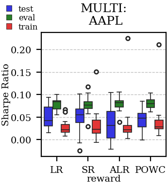
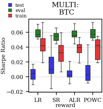
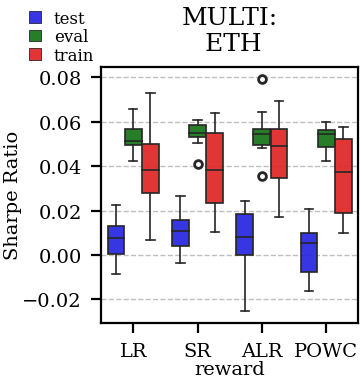
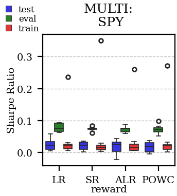
Figure 2. Distribution of the performance of multiple experiments (9, 13, 14, 17) with different random initialization for different assets on training, evaluation and test datasets, with multi reward.

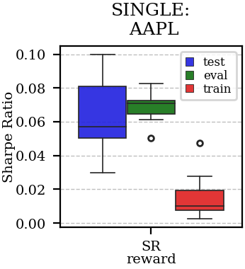
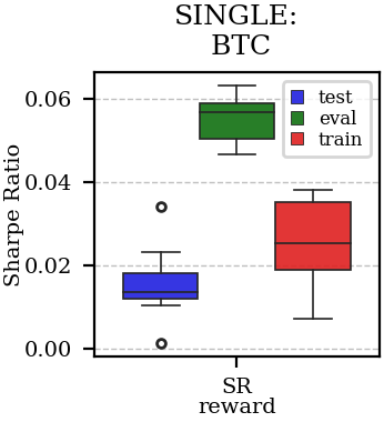
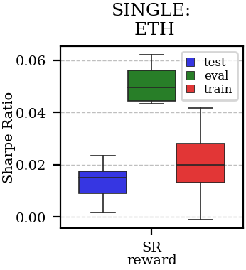
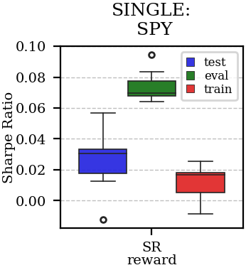
Figure 3. Distribution of the performance of multiple experiments (7, 8) with different random initialization for different assets on training, evaluation and test datasets, with single reward (SR).

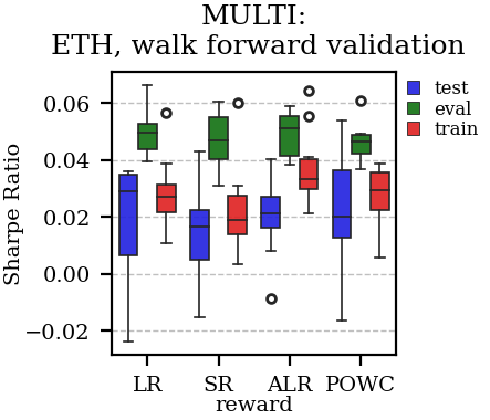
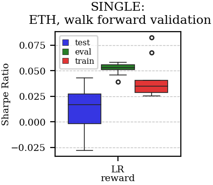
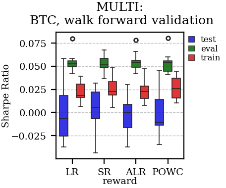
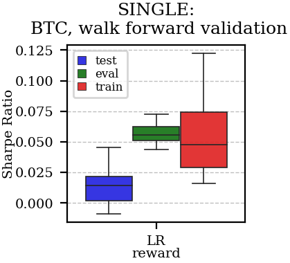
Figure 4. Distribution of the performance of multiple experiments (10) with different random initialization. Results are shown for ETHUSDT and BTCUSD on training, evaluation and test datasets. We compare multi and single reward using anchored walk-forward validation.

Secondly, the generalization is also visible for cumulative rewards in Figures 15 & 16 (Single- vs Multi- for SR metric on BTCUSD and ALR metric on NIFTY50). Thirdly, as far as the predictive power is concerned, the Multi-Reward method is as performing as – and sometimes better performing than – the Single-Reward counterpart, see Figures 17–18–19.

Remark 2.

The training saturation levels may differ from those of the corresponding Single-Reward simulations, although this is likely caused by an apparent regularization effect of the Multi-Reward setting.

Remark 3.

The performance in the case of non-null fees (see Figure 5) is poor: this is not related to the generalization (which seems to hold also in this case), but rather to the simple nature of the underlying RL algorithm, see discussion in Subsection 2.3.3.

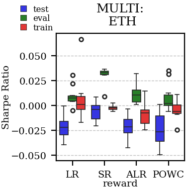
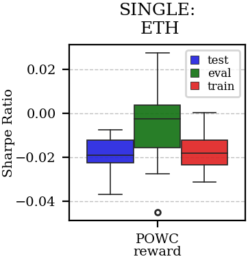
Figure 5. Distribution of the performance of multiple experiments (8, 10) with different random initialization for ETHUSDT on training, evaluation and test datasets, with multi and single (POWC) reward including fees of $0.03\%$.

7.2. Multi-Reward improvement on strongly position-dependent rewards

Let us consider a trading reward which

:

i) is strongly dependent on a specific trading position, and;

:

ii) is sparse (meaning that it might take several time steps for such a reward to return a non-zero value).

Intuition says that it is highly likely that the Single-Reward RL algorithm will struggle to learn based on such a reward. On the other hand, it is expected that a Multi-Reward algorithm will perform better, due to the influence of easier rewards with different but similar goals. Furthermore, the performance difference between Multi-Objective and Single-Objective method is expected to be even more pronounced when there are fewer trading positions allowed (thus further restricting the Single-case capabilities to learn).

Below, we confirm these intuitions for the POWC reward – which satisfies i) and ii) above – by running the Multi-Reward RL code with all four rewards considered in Subsection 5.3 in its dictionary.

7.2.1. Case LP

When opening Short positions is not allowed, the POWC reward provides a non-zero feedback only when Long positions are closed. This extremely sparse feedback is likely to be the justification of the poor cumulative training performance (Figures 6 and 7) where Single-Reward saturates the training at a much lower level than Multi-Reward. In contrast, the training for the Multi-case algorithm is much more consistent, as it can benefit from rewards with similar goals as POWC, but with more frequent feedback (e.g., LR). In the Multi-Reward case, the prediction performance exceeds the Buy-and-Hold threshold on the BTCUSD dataset in a more consistent and stable way than in the training saturation regime of the Single-Reward case. Furthermore, the average of Long positions is lower (which means less risk is taken) and are also relatively stable. The difference in strategy between Multi and Single-Reward algorithm can be inferred by the different convergence of Long Positions. The analysis is further consolidated by considering the stark contrast in saturation levels in the distributional plots for the XRPUSDT and ETHUSDT, see Figures 8–9.

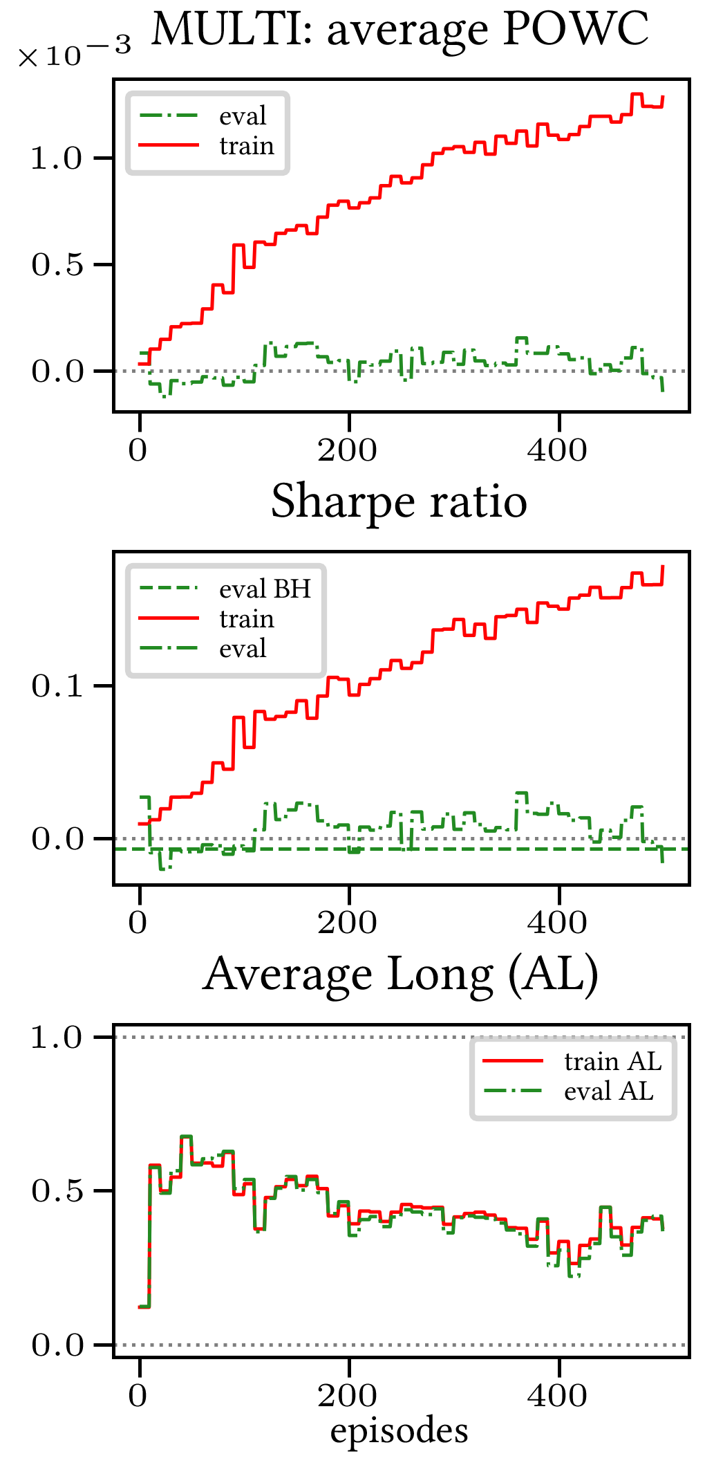
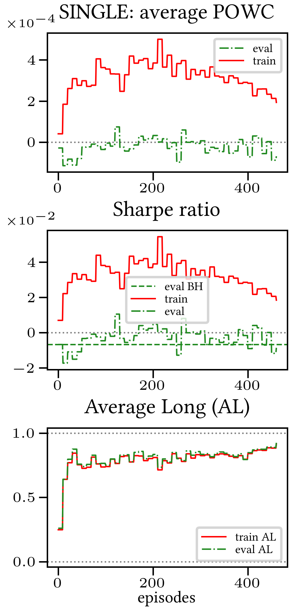
Figure 6. Reward performances, POWC/LP/BTCUSDT

POWCRewardsLP

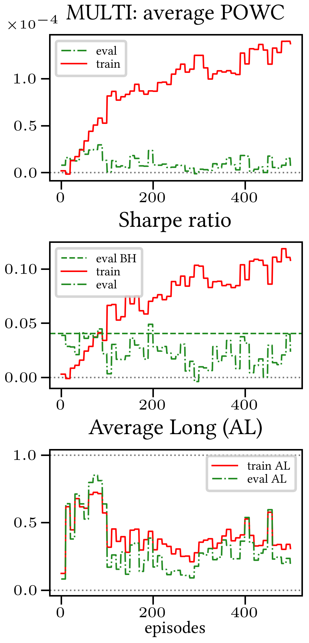
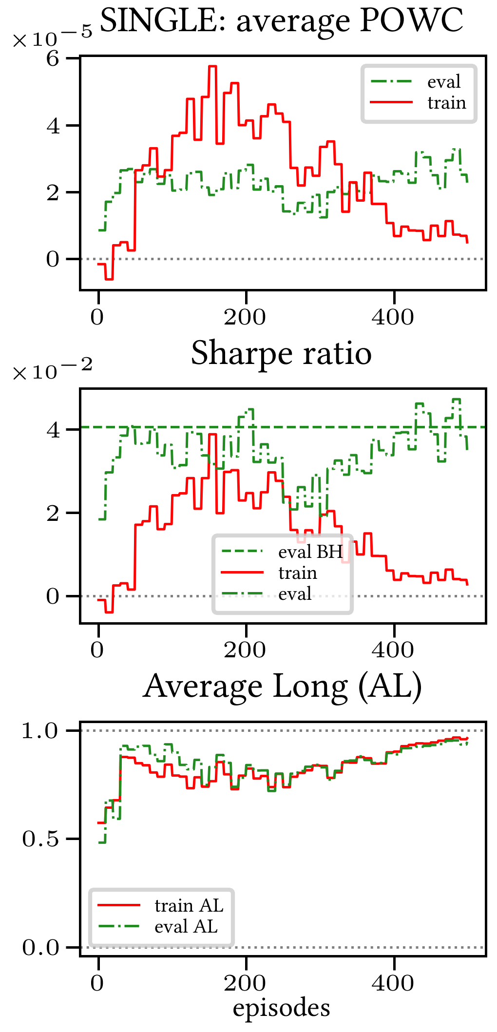
Figure 7. Reward performances, POWC/LP/NIFTY50

POWCRewardsLPNifty

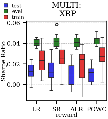
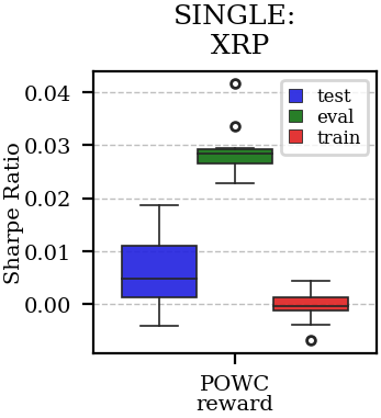
Figure 8. LP case: Distribution of the performance of multiple experiments with different random initialization for XRPUSDT and POWC on training, evaluation and test datasets, with multi and single reward.

POWCRewardsXRPBoxplots

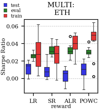
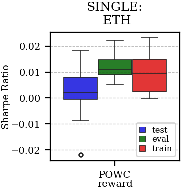
Figure 9. LP case: Distribution of the performance of multiple experiments with different random initialization for ETHUSDT and POWC on training, evaluation and test datasets, with multi and single reward.

POWCRewardsETHBoxplots

7.2.2. Case L&SP

As expected, the difference between Multi- and Single- case is much narrower in this case, as Short positions can now be opened, see Figures 11 and 12. Except for the training saturation, relevant differences are not noted. This is also visible in distributional plots (for instance, consider the SPY pair in Figures 2 and 10).

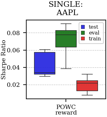
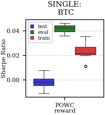
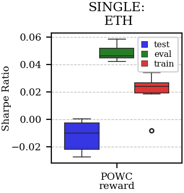
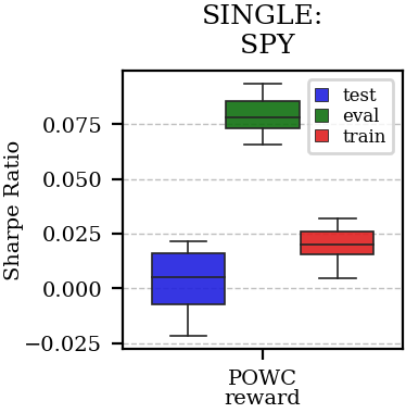
Figure 10. Distribution of the performance of multiple experiments (7) with different random initialization for different assets on training, evaluation and test datasets, with single reward (POWC).

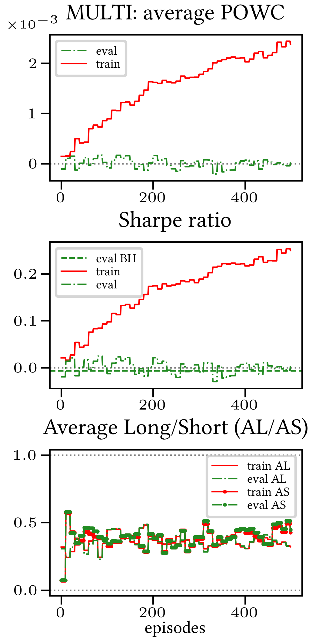
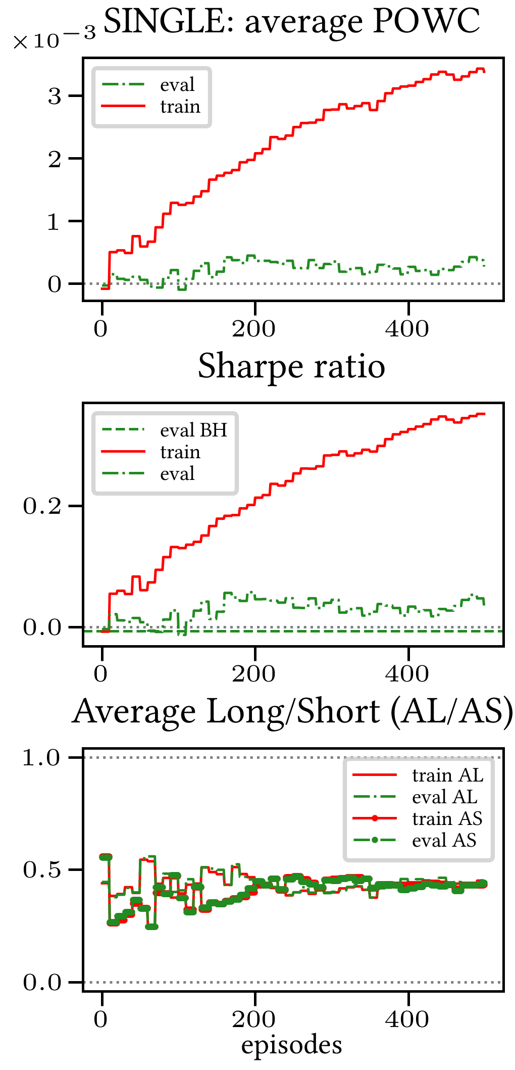
Figure 11. Reward performances, POWC/L&SP/BTCUSDT

POWCRewardsLSP

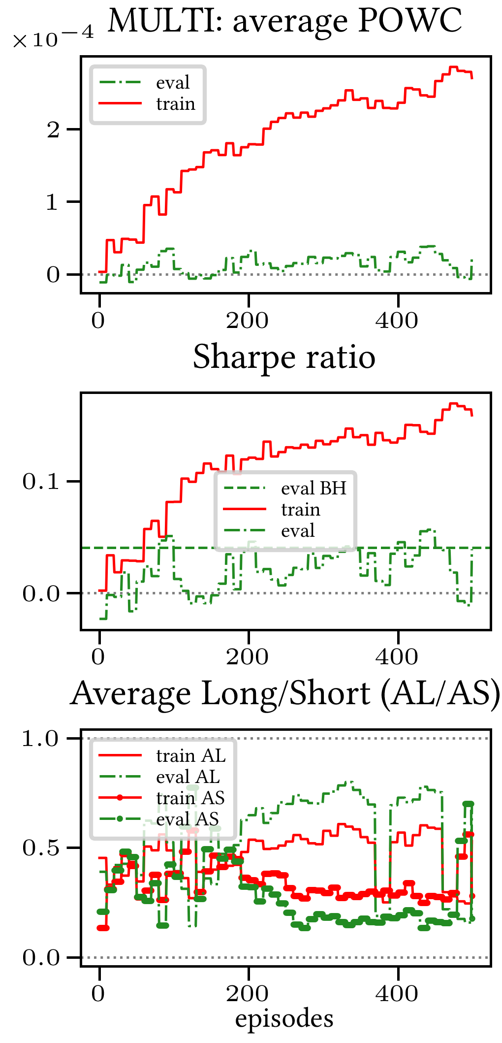
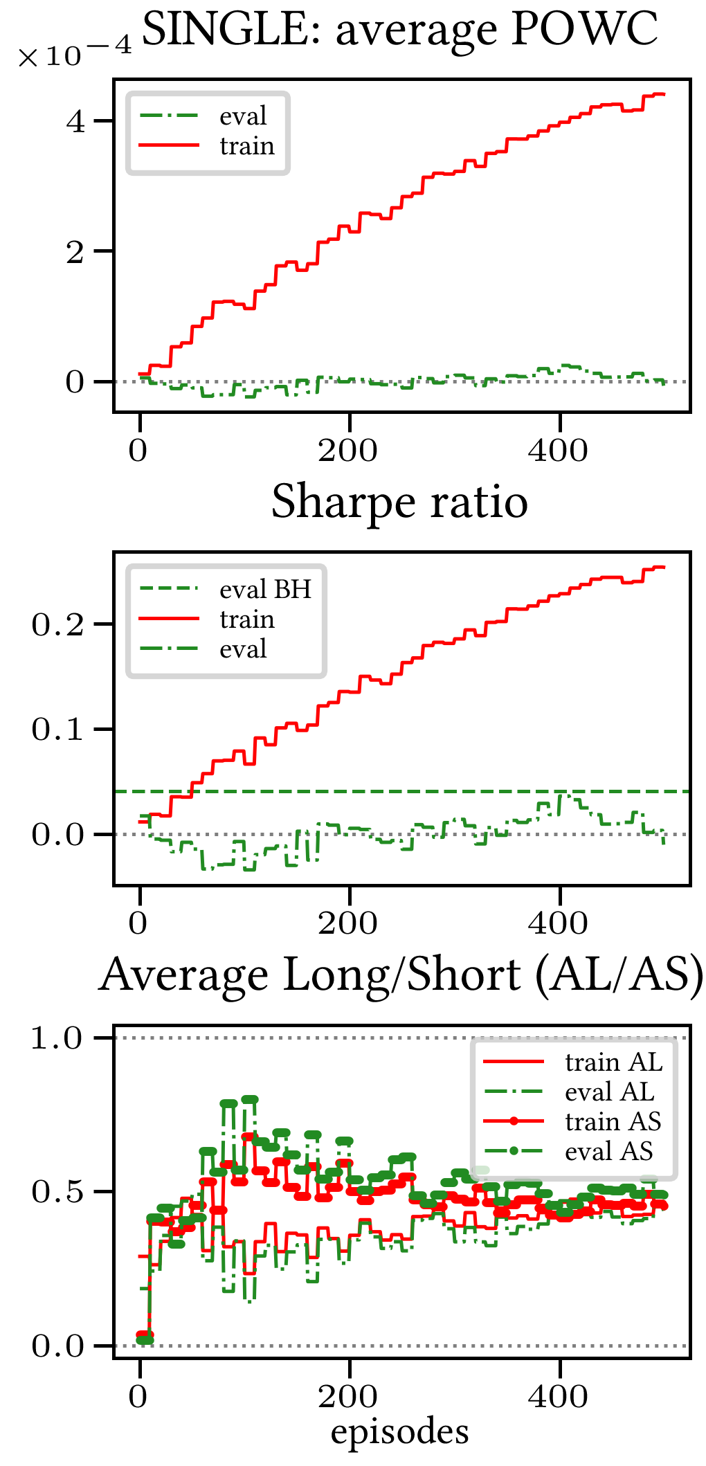
Figure 12. Reward performances, POWC/L&SP/NIFTY50

POWCRewardsLSPNifty

7.3. Random discount factor generalization

We have run several simulations with both fixed and randomly sampled discount factor (as suggested in (Friedman and Fontaine, 2018)) on all datasets. The results are consistent across all simulations: therefore, we only show the results for the BTCUSD dataset in Figures 13 and 14 (Multi-Reward case only, for reward SR in both the LP and L&SP cases), as they are representative of all the remaining simulations.

We were able to notice the following general trends:

:

- Generalization. A graphical comparison of performance indicators suggests that the algorithm generalizes with respect to the value of the random discount factor.

:

- Training saturation levels. There is a visible difference of saturation levels, with the random discount factor version saturating at a consistently lower level than its non-random discount factor counterpart. It is plausible that the discount factor generalization serves the purpose of a neural network regularizer. The difference is more pronounced in the L&SP case, i.e., when the agent is allowed to open Short positions.

:

- Evaluation set saturation levels and average positions. No significant differences are noticeable between the two cases.

Taking everything into account, our simulations point in the direction of validating the discount factor generalization assumption provided in (Friedman and Fontaine, 2018). Nevertheless, more extensive testing is necessary in order to fully confirm this.

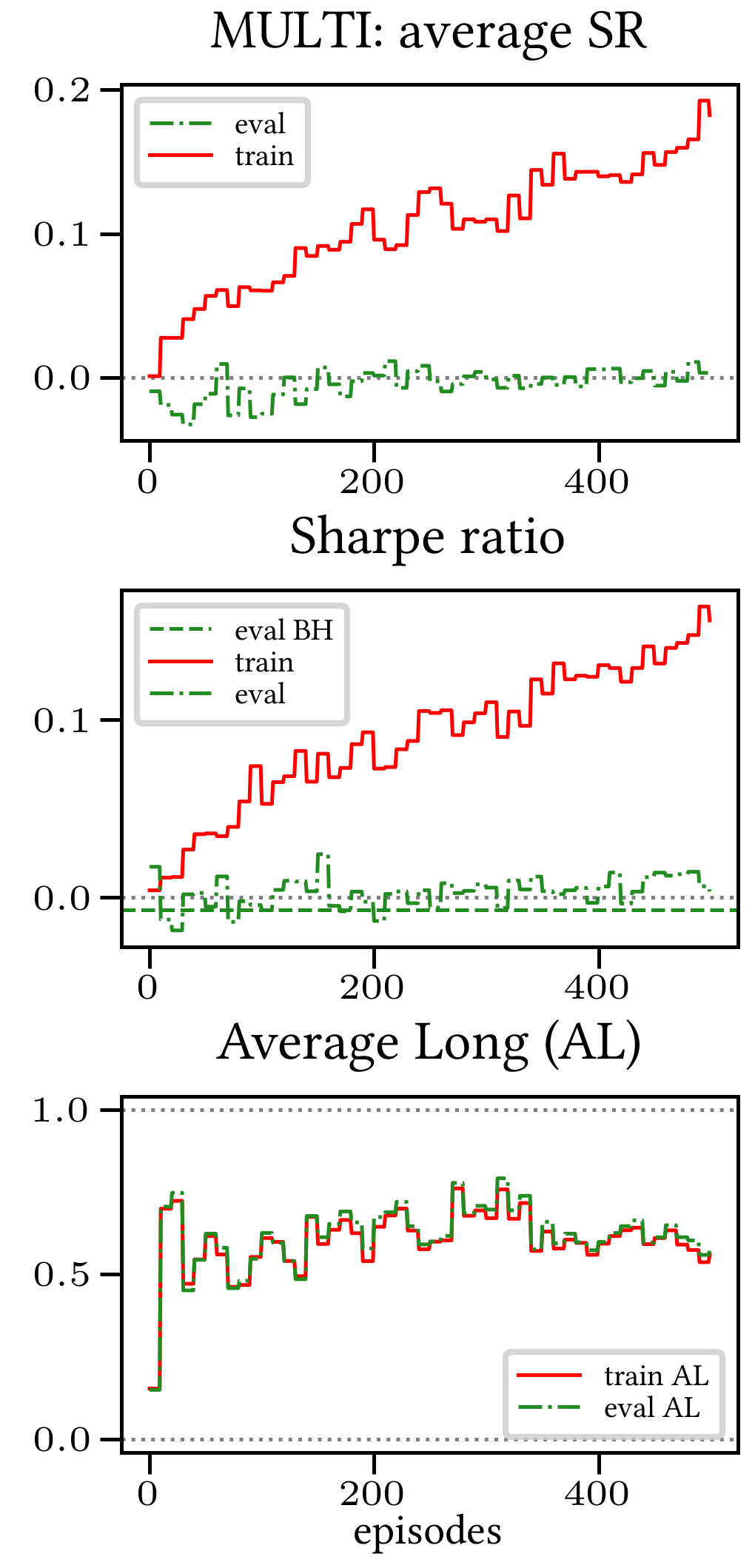
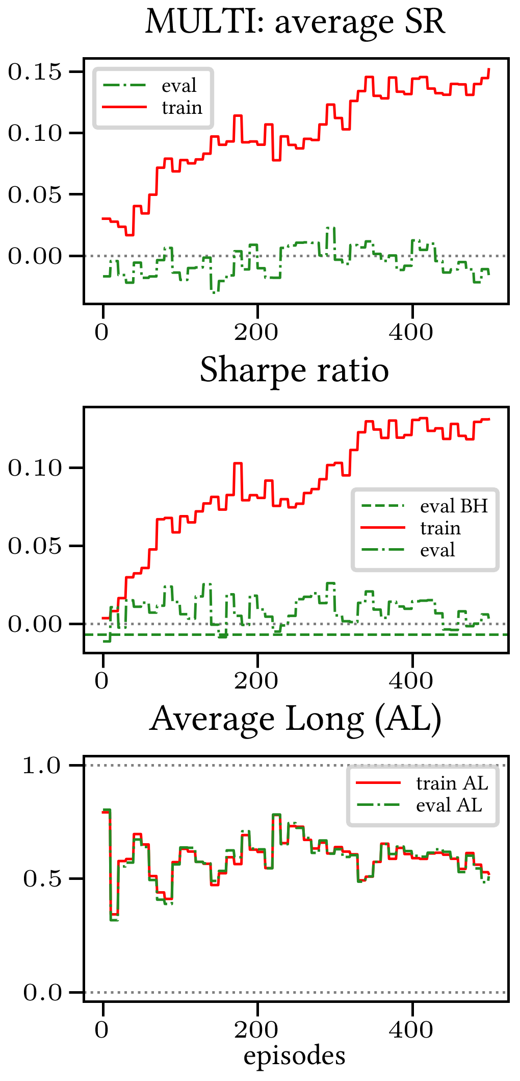
Figure 13. Reward Performances, SR/LP/BTCUSDT. Left (Right): Non-random (Random) discount factor

rgammaRewardsLP-SR

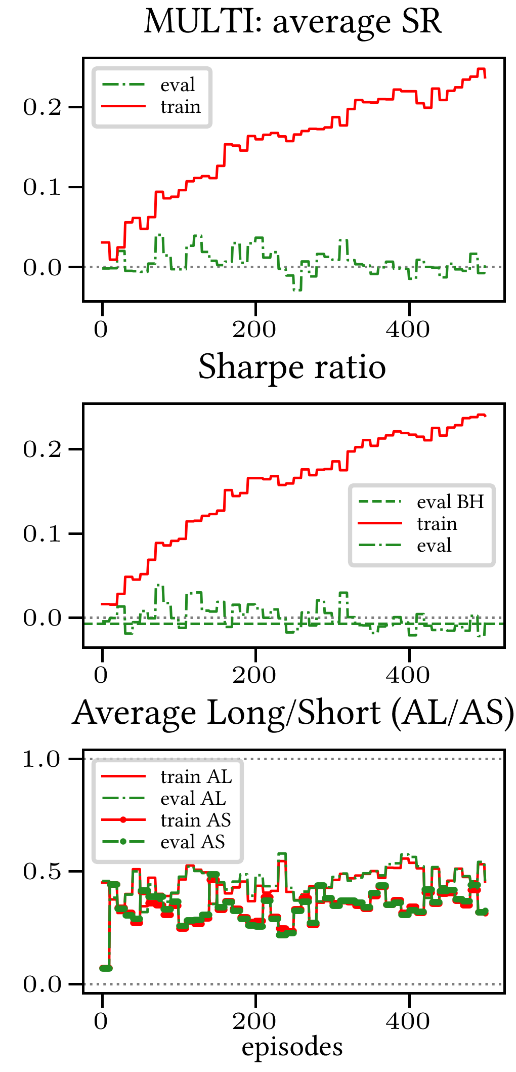
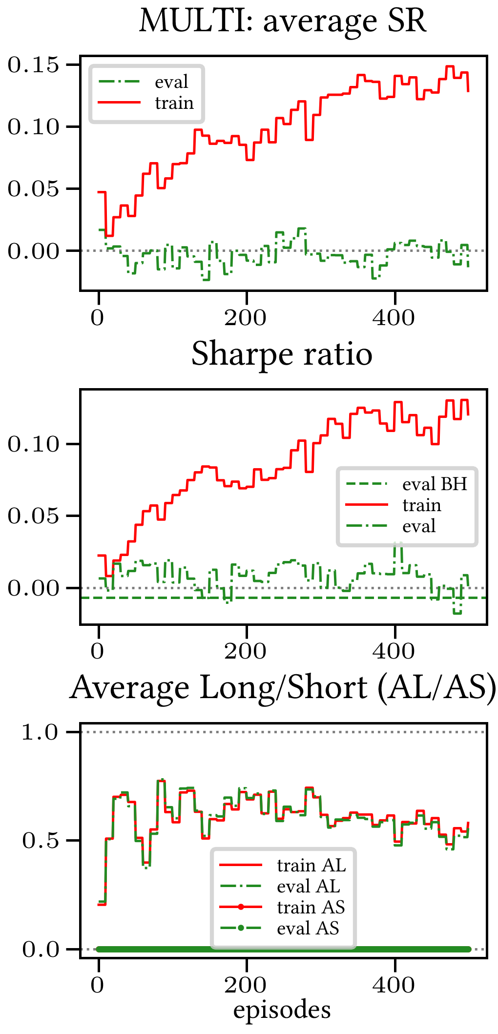
Figure 14. Reward Performances, SR/L&SP/BTCUSDT. Left (Right): Non-random (Random) discount factor

rgammaRewardsLSP-SR

7.4. Consistent indications for predictability

Although a full statistical justification of the obtained results is beyond the scope of this paper, we nonetheless have achieved indications that validate the effectiveness and robustness of the Multi-Reward approach. We further detail this statement.

7.4.1. Consistent performance with respect to the Buy-and-Hold strategy

In the majority of simulations, the Multi-Reward is capable of improving over the Buy-and-Hold strategy benchmark (in terms of Sharpe ratio), on the evaluation and, more importantly, on the test set (Figure 20). Our validation has primarily relied on a distributional analysis across several experiments with independent initialization (Figures 2, 3, 4, 10, 20).

7.4.2. Comparing performance on training, evaluation, test sets

A commonly used model selection strategy is to pick the best performing model on the evaluation set. In Figures 17, 18, 19, the performance of such best performing model is shown (for training, evaluation, test) as it progresses through the episodes. We observe that the performance on the evaluation set (in terms of the Sharpe Ratio) is consistently good. In particular, the performance of the Multi-Reward model is at least as good as that of the Single-Reward model, while also being much more stable. Furthermore, the profits on the test sets are higher and more consistent in the Multi-Reward case (especially in the case of NIFTY50, see Figure 19). The results in Figures 17, 18, 19 also show that the performance on the test set is loosely correlated with the one on the evaluation set. This is likely due to the noisiness of the learning process, and a neat difference between evaluation and test set. In any case, the performance on the evaluation is a reliable indication for the improved stability, as it depends on the stability of the learning process.

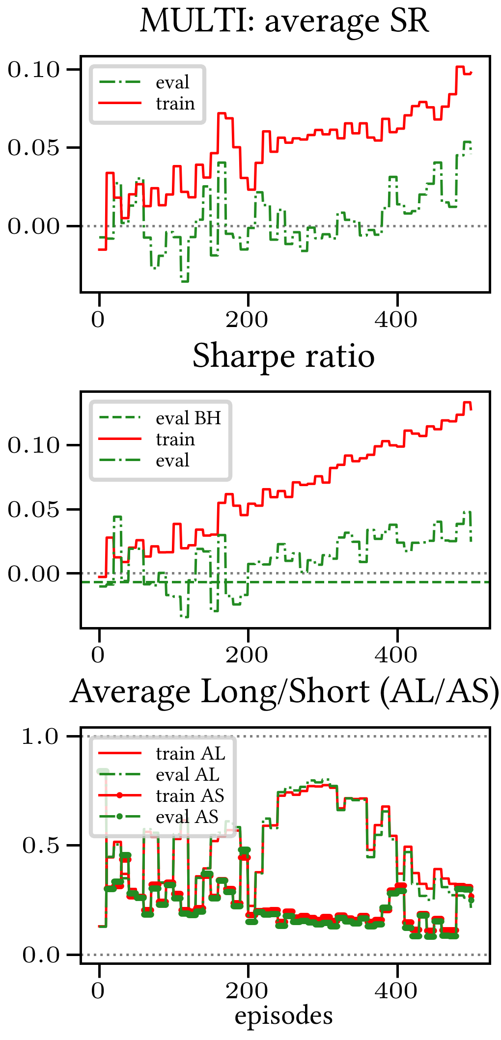
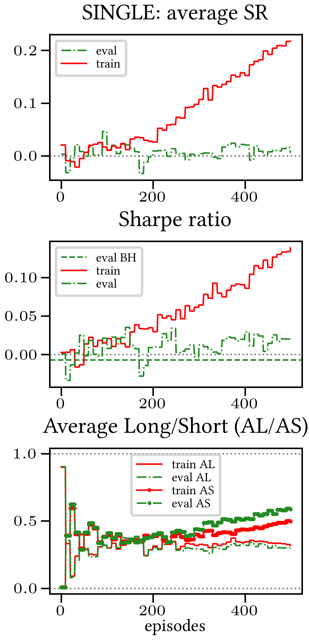
Figure 15. Reward Performances, SR/L&SP/BTCUSDT, regularized agent’s network

pred1

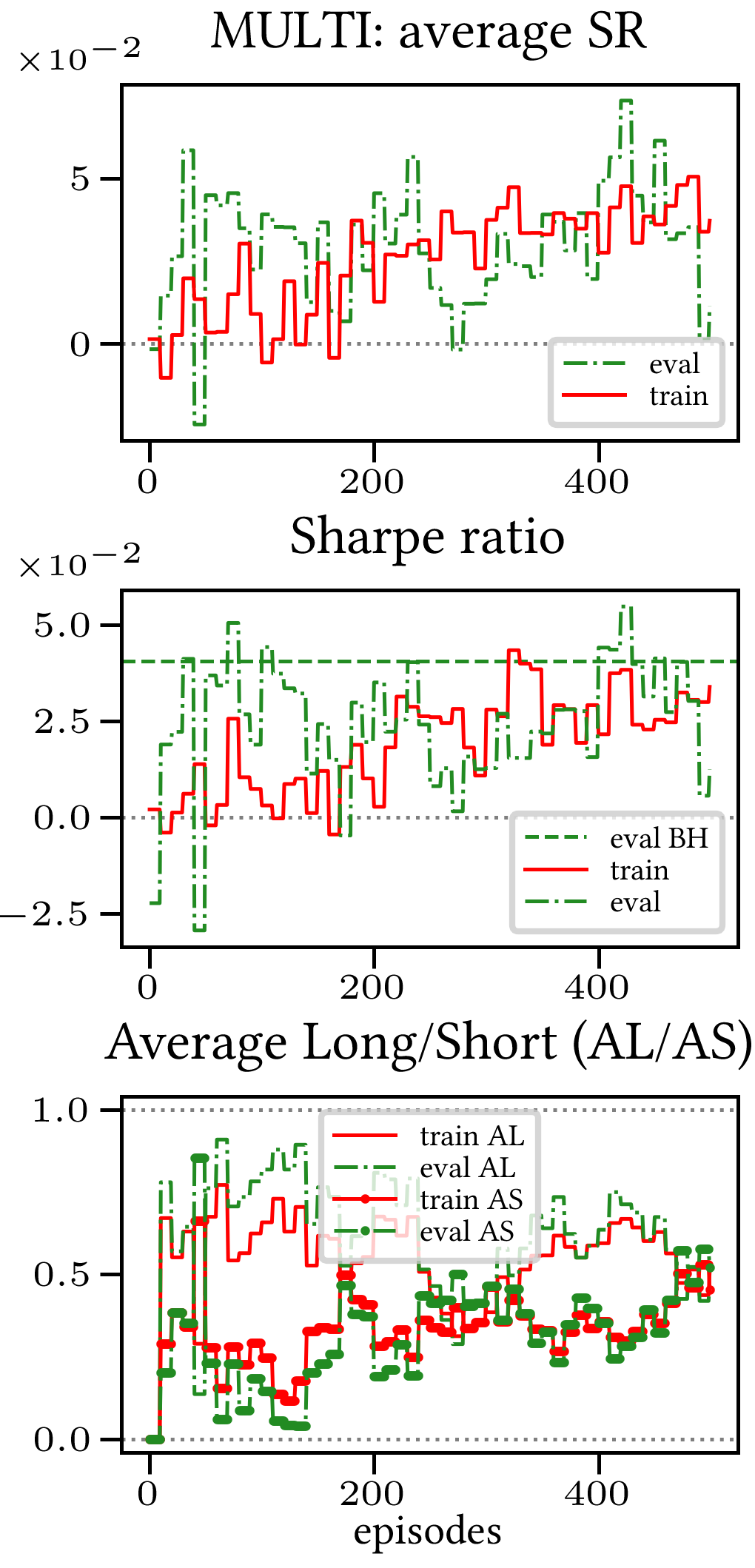
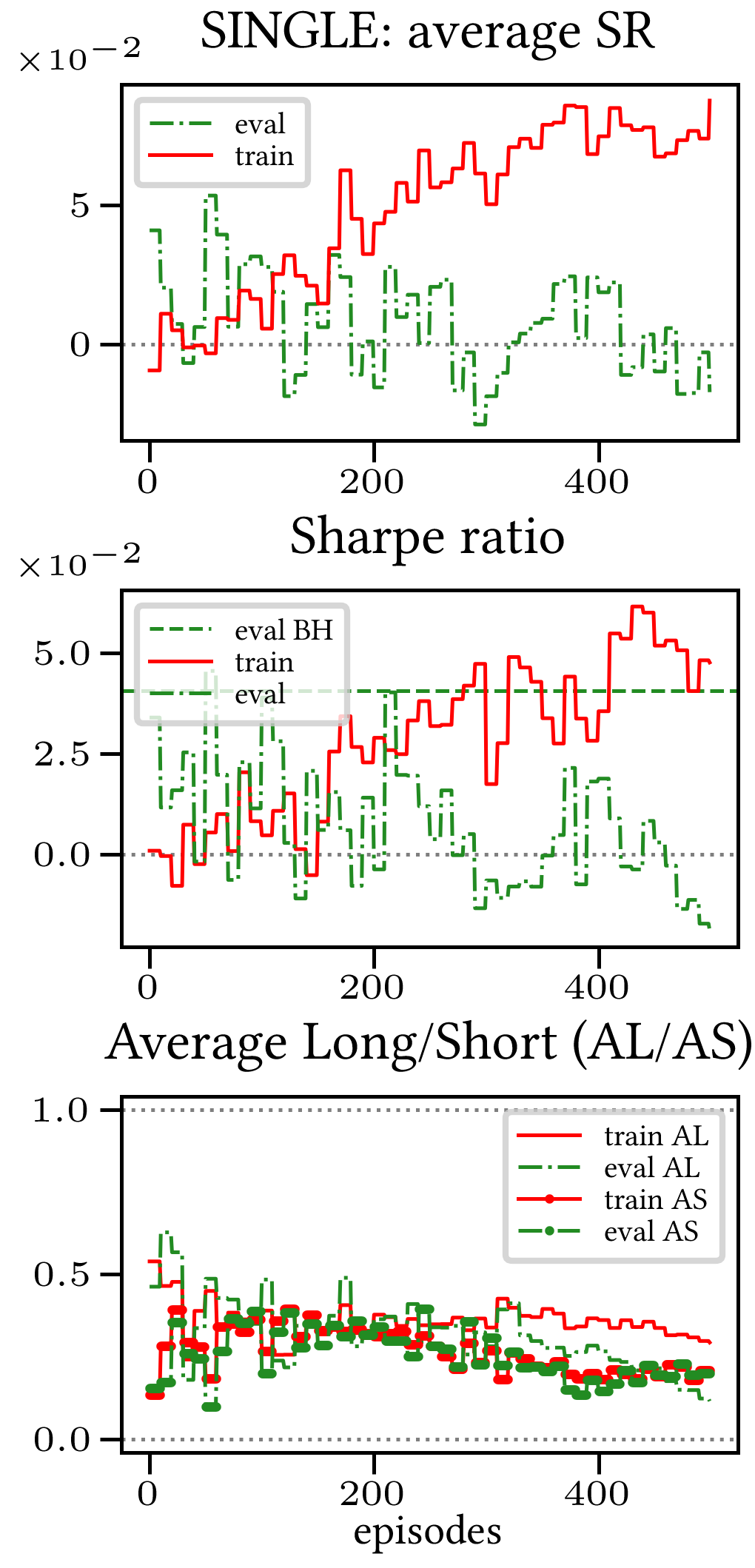
Figure 16. Reward Performances, ALR/L&SP/NIFTY50, regularized agent’s network

pred2

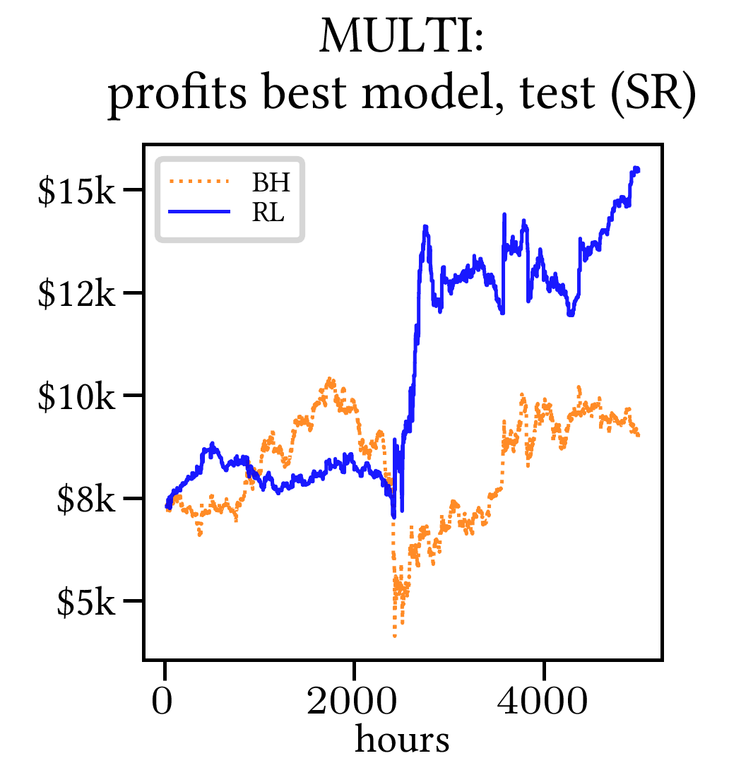
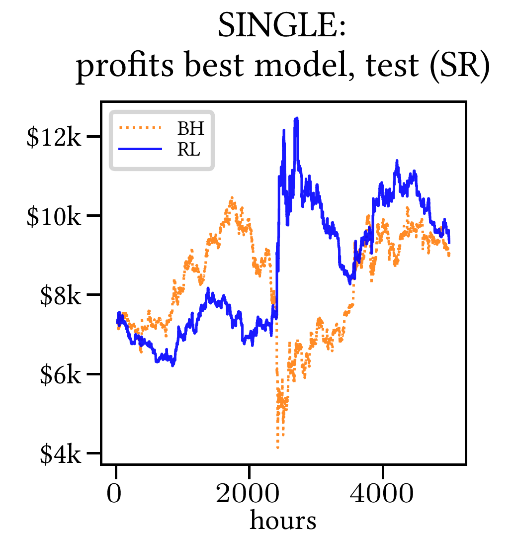
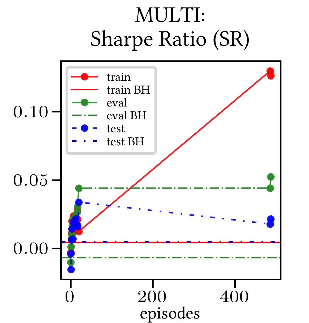
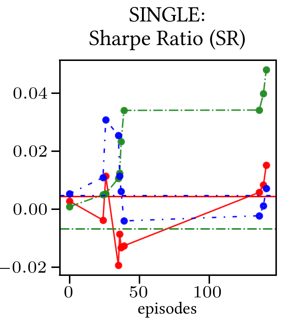
Figure 17. Top (Bottom): Best model for profits (performance for training/evaluation/test set based on SR), BTCUSD

ADD DESCRIPTION

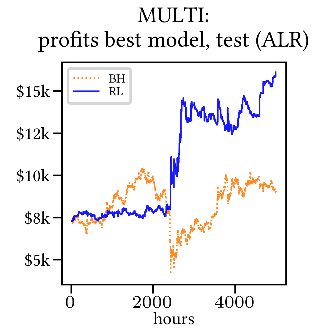
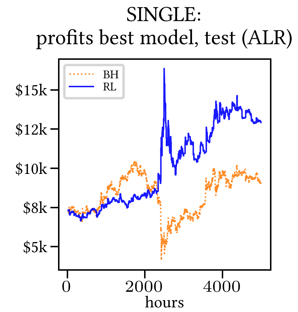
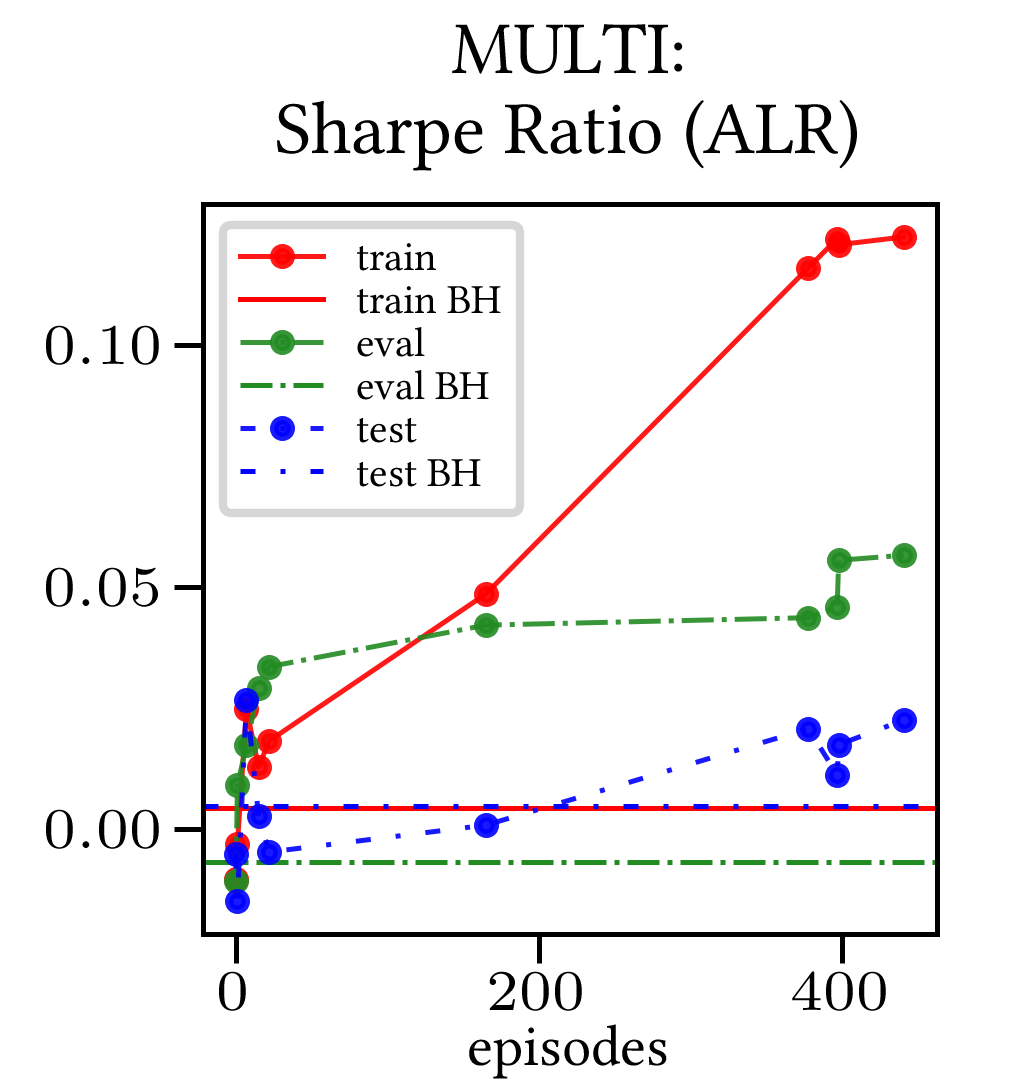
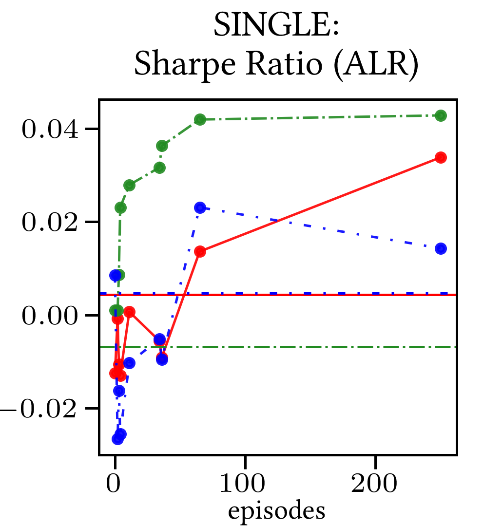
Figure 18. Top (Bottom): Best model for profits (performance for training/evaluation/test set based on ALR), BTCUSD

ADD DESCRIPTION

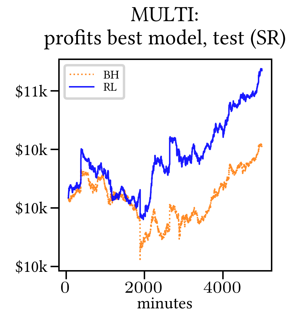
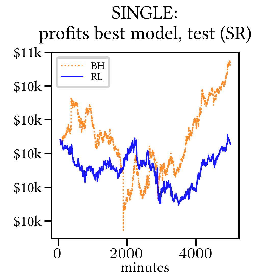
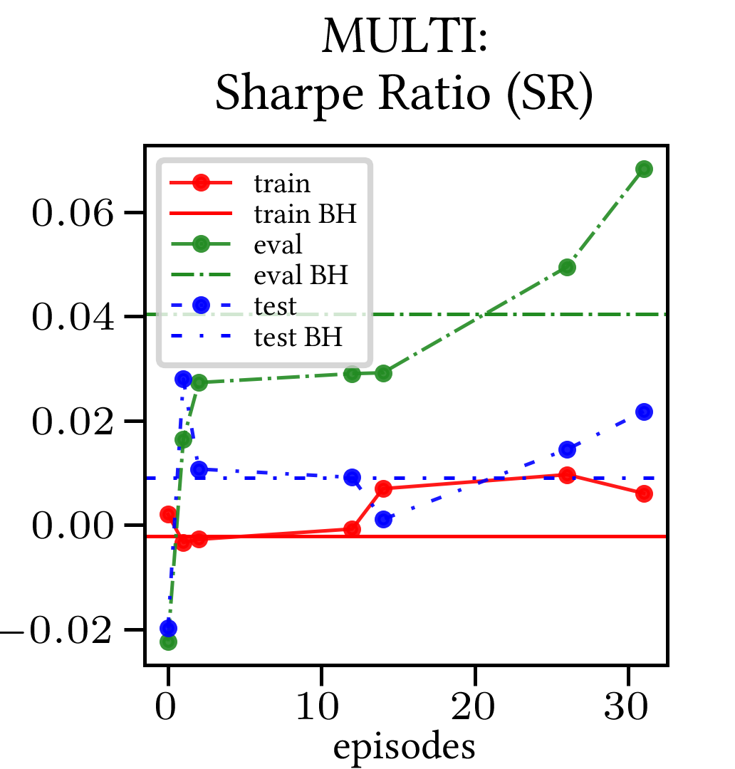
Figure 19. Top (Bottom): Best model for profits (performance for training/evaluation/test set based on SR), NIFTY50

ADD DESCRIPTION

Figure 20. Distribution of the performance of multiple experiments with different random initialization for BTCUSD and AAPL on training, evaluation and test datasets, with multi and single reward.

8. Conclusions

Firstly, we have validated the generalization properties of a Multi-Reward, Reinforcement Learning method with Hindsight Experience Replay (in the declination given by (Friedman and Fontaine, 2018)) by running experiments on several important, single-asset datasets (AAPL, SPY, ETHUSDT, XRPUSDT, BTCUSD, NIFTY50).

Secondly, even though a full statistical analysis would require further work, we have provided a number of consistent statistical indicators confirming the improved stability of our Multi-Reward method over its Single-Reward counterpart: distribution of performance over independent runs, convergence of prediction indicators, and profits for best performing models.

Thirdly, we verified that the Multi-Reward has a clear edge over its Single-Reward counterparts in the case of sparse, heavily position-dependent reward mechanisms.

Finally, we have partially validated the generalization property regarding the discount factor (as suggested by (Friedman and Fontaine, 2018)), even though more work is required to consolidate the claim.

8.1. Limits of the RL setting

The obtained results are, in nearly all occasions, subject to noise: more specifically, relevant performance indicators occasionally oscillate around – rather than approach – their limiting value (with respect to the number of epochs). This behavior, which is visible in the cumulative reward plots (Figures 11–12–13–14–15–16), is consistent with what can be expected from a critic-only Reinforcement Learning approach. Additionally, despite the (not at all short) length of training, evaluation, and test set, the data is obviously correlated in time, thus the effectiveness of the method is reduced. The impact of the noise is mitigated by running several experiments (Figures 2, 3, 4, 10, 20).

9. Future Outlook

While we have highlighted some of the benefits that a Multi-Reward approach has over a Single-Reward approach for predictive properties of a critic-only RL paradigm for single-asset financial data, many questions remain partially answered, or even wide open.

Firstly, while the Multi-Reward approach can stabilize and improve results of some rewards using the other ones, it is not clear exactly how the rewards are influenced by each other (normalization approaches different from (3) could be investigated). Secondly, it would be interesting to conduct a more thorough research into different lengths and non-uniform sampling mechanisms for the experience replay (see (Fedus et al., 2020)). Thirdly, a more thorough analysis on the use of a random discount factor should be conducted. Fourthly, one might perform a sensitivity analysis on more hyperparameters. Fifthly, a more in depth analysis of the prediction power to provide statistical evidence is still needed. Finally, it would be interesting to further address the noisy convergence of the performance metrics (see Section 8.1).

Appendix A RL algorithms

The original Multi-Objective critic-only RL algorithm of Fontaine and Friedman (Friedman and Fontaine, 2018) in summarized in Algorithm 1, while our modified method (inclusive of, among others, random access point and discount factor generalization, see Subsection 4.2) is reported in Algorithm 2 (only the changes against Algorithm 1 are highlighted).

Algorithm 1 (DQN-HER)

Input: MultiReward $\in\{\mbox{True, False}\}$
Parameters: ${\tt tol}\in(0,1)$, ${\tt batchsize},k,M\in\mathbb{N}$, $S\subset\{1,\dots,M\}$
Output: Trained Multi-Reward agent.

1:  Take one-hot encoding vector $\boldsymbol{w}$.

2:  Initialize network $Q\colon(\boldsymbol{s},\boldsymbol{w})\mapsto[Q_{1}(\boldsymbol{s},\boldsymbol{w}),\dots,Q_{P}(\boldsymbol{s},\boldsymbol{w})]$ mapping state variables $\boldsymbol{s}$ and weight vector $\boldsymbol{w}$ to expected discounted return of every action $a\in\{1,\dots,P\}$.

3:  for $i=1,\dots,M$  do

4:     Reset training environment.

5:     while Episode $i$ not finished do

6:        if MultiReward is True then

7:           Sample random reward weights $\boldsymbol{w}$.

8:        end if

9:        if Unif$(0,1)<tol$ then

10:           Choose random action $a$

11:        else

12:           Pick $a\leftarrow\arg\max_{a}{Q(\boldsymbol{s},\boldsymbol{w})}$.

13:        end if

14:        Conduct one step (get to new state $\boldsymbol{s}_{new}$)

15:        Get associated reward $\boldsymbol{w}\cdot\boldsymbol{r}(\boldsymbol{s},a)$

16:        Append single experience $(\boldsymbol{s},\boldsymbol{w},\boldsymbol{w}\cdot\boldsymbol{r}(\boldsymbol{s},a),a,\boldsymbol{s}_{new})$ to experience replay $\mathcal{R}$

17:        Set $\boldsymbol{s}\leftarrow\boldsymbol{s}_{new}$

18:        if MultiReward is True then

19:           Add other $k$ experiences to Replay by re-running lines 7-14-15-16 $k$ times.

20:        end if

21:        if $i\in S$ then

22:           Randomly sample batchsize units from $\mathcal{R}$.

23:           Update $Q$-values associated with each sampled unit using Bellman equation (4.1).

24:           Fit model on estimated $Q$-values

25:        end if

26:     end while

27:  end for

Algorithm 2 (DQN-HER) with discount factor generalization and random access point (Changes to lines of Algorithm 1)

Input: Anchoring for cross-validation $\in\{\mbox{True; False}\}$

2:  Initialize network $Q\colon(\boldsymbol{s},\boldsymbol{w},\gamma)\mapsto[Q_{1}(\boldsymbol{s},\boldsymbol{w},\gamma),\dots,Q_{P}(\boldsymbol{s},\boldsymbol{w},\gamma)]$ mapping state variables $\boldsymbol{s}$, weight vector $\boldsymbol{w}$, and discount factor $\gamma$ to expected discounted return of every action $a\in\{1,\dots,P\}$. $\vdots$

4:  if not Anchoring for cross-validation then

5:     Randomly select subset of training set, and reset associated environment.

6:  end if $\vdots$

7:  Sample random reward weights $\boldsymbol{w}$ and discount factor $\gamma$. $\vdots$

12:  Pick $a\leftarrow\arg\max_{a}{Q(\boldsymbol{s},\boldsymbol{w},\gamma)}$. $\vdots$

16:  Append single experience $(\boldsymbol{s},\gamma,\boldsymbol{w},\boldsymbol{w}\cdot\boldsymbol{r}(\boldsymbol{s},a),a,\boldsymbol{s}_{new})$ to experience replay $\mathcal{R}$ $\vdots$

22:  Randomly sample batchsize units from $\mathcal{R}$, and normalize sampled $Q$-values according to Subsection 4.2.1.

References

- (1)
- Abels et al. (2019) Axel Abels, Diederik Roijers, Tom Lenaerts, Ann Nowé, and Denis Steckelmacher. 2019. Dynamic weights in multi-objective deep reinforcement learning. In International Conference on Machine Learning. PMLR, 11–20.
- Andrychowicz et al. (2017) Marcin Andrychowicz, Filip Wolski, Alex Ray, Jonas Schneider, Rachel Fong, Peter Welinder, Bob McGrew, Josh Tobin, OpenAI Pieter Abbeel, and Wojciech Zaremba. 2017. Hindsight experience replay. Advances in neural information processing systems 30 (2017).
- Barrett and Narayanan (2008) Leon Barrett and Srini Narayanan. 2008. Learning all optimal policies with multiple criteria. In Proceedings of the 25th international conference on Machine learning. 41–47.
- Bekiros (2010) Stelios D Bekiros. 2010. Heterogeneous trading strategies with adaptive fuzzy actor–critic reinforcement learning: A behavioral approach. Journal of Economic Dynamics and Control 34, 6 (2010), 1153–1170.
- Bisht and Kumar (2020) Kiran Bisht and Arun Kumar. 2020. Deep Reinforcement Learning based Multi-Objective Systems for Financial Trading. In 2020 5th IEEE International Conference on Recent Advances and Innovations in Engineering (ICRAIE). IEEE, 1–6.
- Castelletti et al. (2012) Andrea Castelletti, Francesca Pianosi, and Marcello Restelli. 2012. Tree-based fitted Q-iteration for multi-objective Markov decision problems. In The 2012 international joint conference on neural networks (IJCNN). IEEE, 1–8.
- Chan and Shelton (2001) Nicholas T. Chan and Christian Shelton. 2001. An Adaptive Electronic Market-Maker. Computing in Economics and Finance 2001 146. Society for Computational Economics. https://EconPapers.repec.org/RePEc:sce:scecf1:146
- Corazza and Bertoluzzo (2014) Marco Corazza and Francesco Bertoluzzo. 2014. Q-Learning-based financial trading systems with applications. Working Papers 2014:15. Department of Economics, University of Venice ”Ca’ Foscari”. https://EconPapers.repec.org/RePEc:ven:wpaper:2014:15
- Dempster and Leemans (2006) Michael AH Dempster and Vasco Leemans. 2006. An automated FX trading system using adaptive reinforcement learning. Expert Systems with Applications 30, 3 (2006), 543–552.
- Dempster et al. (2001) Michael AH Dempster, Tom W Payne, Yazann Romahi, and Giles WP Thompson. 2001. Computational learning techniques for intraday FX trading using popular technical indicators. IEEE Transactions on neural networks 12, 4 (2001), 744–754.
- Deng et al. (2016) Yue Deng, Feng Bao, Youyong Kong, Zhiquan Ren, and Qionghai Dai. 2016. Deep direct reinforcement learning for financial signal representation and trading. IEEE transactions on neural networks and learning systems 28, 3 (2016), 653–664.
- Dusparic and Cahill (2009) Ivana Dusparic and Vinny Cahill. 2009. Distributed w-learning: Multi-policy optimization in self-organizing systems. In 2009 Third IEEE international conference on self-adaptive and self-organizing systems. IEEE, 20–29.
- Eilers et al. (2014) Dennis Eilers, Christian L Dunis, Hans-Jörg von Mettenheim, and Michael H Breitner. 2014. Intelligent trading of seasonal effects: A decision support algorithm based on reinforcement learning. Decision support systems 64 (2014), 100–108.
- Ernst et al. (2005) Damien Ernst, Pierre Geurts, and Louis Wehenkel. 2005. Tree-based batch mode reinforcement learning. Journal of Machine Learning Research 6 (2005).
- Fedus et al. (2020) William Fedus, Prajit Ramachandran, Rishabh Agarwal, Yoshua Bengio, Hugo Larochelle, Mark Rowland, and Will Dabney. 2020. Revisiting fundamentals of experience replay. In International Conference on Machine Learning. PMLR, 3061–3071.
- Fischer (2018) Thomas G Fischer. 2018. Reinforcement learning in financial markets-a survey. Technical Report. FAU Discussion Papers in Economics.
- Friedman and Fontaine (2018) Eli Friedman and Fred Fontaine. 2018. Generalizing across multi-objective reward functions in deep reinforcement learning. arXiv preprint arXiv:1809.06364 (2018).
- Gold (2003) Carl Gold. 2003. FX trading via recurrent reinforcement learning. In 2003 IEEE International Conference on Computational Intelligence for Financial Engineering, 2003. Proceedings. IEEE, 363–370.
- Gu et al. (2011) Yunqing Gu, Shingo Mabu, Yang Yang, Jianhua Li, and Kotaro Hirasawa. 2011. Trading rules on stock markets using Genetic Network Programming-Sarsa learning with plural subroutines. In SICE Annual Conference 2011. IEEE, 143–148.
- Jangmin et al. (2006) O Jangmin, Jongwoo Lee, Jae Won Lee, and Byoung-Tak Zhang. 2006. Adaptive stock trading with dynamic asset allocation using reinforcement learning. Information Sciences 176, 15 (2006), 2121–2147.
- Jiang et al. (2017) Zhengyao Jiang, Dixing Xu, and Jinjun Liang. 2017. A deep reinforcement learning framework for the financial portfolio management problem. arXiv preprint arXiv:1706.10059 (2017).
- Jin and El-Saawy (2016) Olivier Jin and Hamza El-Saawy. 2016. Portfolio management using reinforcement learning. Stanford University (2016).
- Källström and Heintz (2019) Johan Källström and Fredrik Heintz. 2019. Tunable dynamics in agent-based simulation using multi-objective reinforcement learning. In Adaptive and Learning Agents Workshop (ALA-19) at AAMAS, Montreal, Canada, May 13-14, 2019. 1–7.
- Kaur (2017) S Kaur. 2017. Algorithmic trading using reinforcement learning augmented with hidden Markov model. Technical Report. Working paper, Stanford University.
- Kober et al. (2013) Jens Kober, J Andrew Bagnell, and Jan Peters. 2013. Reinforcement learning in robotics: A survey. The International Journal of Robotics Research 32, 11 (2013), 1238–1274.
- Lee and Jangmin (2002) Jae Won Lee and O Jangmin. 2002. A multi-agent Q-learning framework for optimizing stock trading systems. In International Conference on Database and Expert Systems Applications. Springer, 153–162.
- Lee et al. (2007) Jae Won Lee, Jonghun Park, O Jangmin, Jongwoo Lee, and Euyseok Hong. 2007. A multiagent approach to -learning for daily stock trading. IEEE Transactions on Systems, Man, and Cybernetics-Part A: Systems and Humans 37, 6 (2007), 864–877.
- Lee et al. (2002) Jae Won Lee, Byoung-Tak Zhang, et al. 2002. Stock trading system using reinforcement learning with cooperative agents. In Proceedings of the Nineteenth International Conference on Machine Learning. 451–458.
- Li et al. (2007) Hailin Li, Cihan H Dagli, and David Enke. 2007. Short-term stock market timing prediction under reinforcement learning schemes. In 2007 IEEE International Symposium on Approximate Dynamic Programming and Reinforcement Learning. IEEE, 233–240.
- Mao et al. (2016) Hongzi Mao, Mohammad Alizadeh, Ishai Menache, and Srikanth Kandula. 2016. Resource management with deep reinforcement learning. In Proceedings of the 15th ACM workshop on hot topics in networks. 50–56.
- Mnih et al. (2013) Volodymyr Mnih, Koray Kavukcuoglu, David Silver, Alex Graves, Ioannis Antonoglou, Daan Wierstra, and Martin Riedmiller. 2013. Playing atari with deep reinforcement learning. arXiv preprint arXiv:1312.5602 (2013).
- Moody et al. (1998) John Moody, Lizhong Wu, Yuansong Liao, and Matthew Saffell. 1998. Performance functions and reinforcement learning for trading systems and portfolios. Journal of Forecasting 17, 5-6 (1998), 441–470.
- Mossalam et al. (2016) Hossam Mossalam, Yannis M Assael, Diederik M Roijers, and Shimon Whiteson. 2016. Multi-objective deep reinforcement learning. arXiv preprint arXiv:1610.02707 (2016).
- Natarajan and Tadepalli (2005) Sriraam Natarajan and Prasad Tadepalli. 2005. Dynamic preferences in multi-criteria reinforcement learning. In Proceedings of the 22nd international conference on Machine learning. 601–608.
- Neuneier (1995) Ralph Neuneier. 1995. Optimal asset allocation using adaptive dynamic programming. Advances in Neural Information Processing Systems 8 (1995).
- Nevmyvaka et al. (2006) Yuriy Nevmyvaka, Yi Feng, and Michael Kearns. 2006. Reinforcement learning for optimized trade execution. In Proceedings of the 23rd international conference on Machine learning. 673–680.
- Nguyen et al. (2020) Thanh Thi Nguyen, Ngoc Duy Nguyen, Peter Vamplew, Saeid Nahavandi, Richard Dazeley, and Chee Peng Lim. 2020. A multi-objective deep reinforcement learning framework. Engineering Applications of Artificial Intelligence 96 (2020), 103915.
- Rădulescu et al. (2020) Roxana Rădulescu, Patrick Mannion, Diederik M Roijers, and Ann Nowé. 2020. Multi-objective multi-agent decision making: a utility-based analysis and survey. Autonomous Agents and Multi-Agent Systems 34, 1 (2020), 1–52.
- Reymond and Nowé (2019) Mathieu Reymond and Ann Nowé. 2019. Pareto-DQN: Approximating the Pareto front in complex multi-objective decision problems. In Proceedings of the adaptive and learning agents workshop (ALA-19) at AAMAS.
- Roijers et al. (2013) Diederik M Roijers, Peter Vamplew, Shimon Whiteson, and Richard Dazeley. 2013. A survey of multi-objective sequential decision-making. Journal of Artificial Intelligence Research 48 (2013), 67–113.
- Sherstov and Stone (2004) Alexander A Sherstov and Peter Stone. 2004. Three automated stock-trading agents: A comparative study. In International Workshop on Agent-Mediated Electronic Commerce. Springer, 173–187.
- Si et al. (2017) Weiyu Si, Jinke Li, Peng Ding, and Ruonan Rao. 2017. A multi-objective deep reinforcement learning approach for stock index future’s intraday trading. In 2017 10th International symposium on computational intelligence and design (ISCID), Vol. 2. IEEE, 431–436.
- Sutton and Barto (2018) Richard S Sutton and Andrew G Barto. 2018. Reinforcement learning: An introduction. MIT press.
- Tajmajer (2017) Tomasz Tajmajer. 2017. Multi-objective deep Q-learning with subsumption architecture. arXiv preprint arXiv:1704.06676 (2017).
- Tajmajer (2018) Tomasz Tajmajer. 2018. Modular multi-objective deep reinforcement learning with decision values. In 2018 Federated conference on computer science and information systems (FedCSIS). IEEE, 85–93.
- Tan et al. (2011) Zhiyong Tan, Chai Quek, and Philip YK Cheng. 2011. Stock trading with cycles: A financial application of ANFIS and reinforcement learning. Expert Systems with Applications 38, 5 (2011), 4741–4755.
- Watts (2015) Samuel Watts. 2015. Hedging basis risk using reinforcement learning. Technical Report. Technical report, Working Paper, University of Oxford.
- Zheng et al. (2018) Guanjie Zheng, Fuzheng Zhang, Zihan Zheng, Yang Xiang, Nicholas Jing Yuan, Xing Xie, and Zhenhui Li. 2018. DRN: A deep reinforcement learning framework for news recommendation. In Proceedings of the 2018 World Wide Web Conference. 167–176.
- Zitzler et al. (2008) Eckart Zitzler, Joshua Knowles, and Lothar Thiele. 2008. Quality assessment of pareto set approximations. Multiobjective optimization (2008), 373–404.