Spectral Efficiency of Unicast and Multigroup Multicast Transmission in Cell-free Distributed Massive MIMO Systems

Abstract

In this paper, we consider a joint unicast and multi-group multicast cell-free distributed massive multiple-input multiple-output (MIMO) system, while accounting for co-pilot assignment strategy based channel estimation, pilot contamination and different precoding schemes. Under the co-pilot assignment strategy, we derive the minimum-mean-square error (MMSE) channel state information (CSI) estimation for unicast and multicast users. Given the acquired CSI, the closed-form expressions for downlink achievable rates with maximum ratio transmission (MRT), zero-forcing (ZF) and MMSE beamforming are derived. Based on these expressions, we propose an efficient power allocation scheme by solving a multi-objective optimization problem (MOOP) between maximizing the minimum spectral efficiency (SE) of multicast users and maximizing the average SE of unicast users with non-dominated sorting genetic algorithm II (NSGA-II). Moreover, the MOOP is converted into a deep learning (DL) problem and solved by an unsupervised learning method to further promote computational efficiency. Numerical results verify the accuracy of the derived closed-form expressions and the effectiveness of the joint unicast and multigroup multicast transmission scheme in cell-free distributed massive MIMO systems. The SE analysis under various system parameters and the trade-off regions between these two conflicting optimization objectives offers numerous flexibilities for system optimization.

I Introduction

Cell-free distributed massive multiple-input multiple-output (MIMO) systems are practical and scalable scenarios of MIMO network [1, 2, 3]. By reaping the benefits from both massive MIMO and network MIMO systems, cell-free distributed massive MIMO can effectively improve the spectral efficiency (SE), energy efficiency (EE) and reliable data transmission [4, 5, 6]. In cell-free distributed massive MIMO systems, connected to a central processing unit (CPU), a great number of remote antenna units (RAUs) are geographically distributed and coherently serve the users. Compared with centralized massive MIMO, cell-free distributed massive MIMO provides a higher macro-diversity gain and lower proximity, thus achieves better performance [7, 8]. [2] extended the cell-free approach to the case of a user-centric massive MIMO approach and proposed power allocation strategies aimed at either sum-rate maximization or minimum-rate maximization. [9] provided a extensive survey of cell-free massive MIMO systems and discussed the benefits of cell-free massive MIMO systems including energy and cost efficiency. [10] investigated the user-centric cell-free massive MIMO with distributed units to serve users. In such systems, a specific cluster of RAUs is served for each user and the user-centric scheme reduces edging effect, thus help to inprove the coverage and performance for users across the whole network. [11] proposed a cloud-based cell-free distributed massive MIMO system meet 5G NR requirements. [12] revealed the cell-free massive MIMO systems outmatch small-cells design for both coverage and rate because it takes advantage of both network MIMO and classical massive MIMO systems. Uplink SE in cell-free massive MIMO systems is analyzed in [13]. The spacial correlated propagation in cell-free massive MIMO with short-term power constrains is studied in [14]. [15] analyzed the uplink average ergodic capacity and gave a closed-form approximation in distributed massive MIMO. [16] investigated an energy efficiency resource allocation scheme in downlink transmission to maximize system energy efficiency considered power consumption including transmitting power, calculation power and circuit power. [17] proposed an iterative algorithm for maximizing the minimum achievable rate of downlink transmission among the UEs in cell-free massive MIMO. [18] proposesd two power allocation algorithms based on quantizing the downlink transmitted powers of APs for reducing complexity with Conjugate Beamforming (CB) and Zero-Forcing (ZF) precoding. [19] evaluated different trade-offs between precoding strategies, power allocation techniques and pilot allocation strategies affecting the performance in cell-free massive MIMO networks. [20] proposed an method for dividing the pilot power and data power in the downlink transmission to maximize the minimum achievable rate of the users in a cell-free massive MIMO system. [21] proposed a new FP-based algorithm for spectral efficiency power allocation to solve several convex problems with closed-form solutions.[22] studied the power control and allocation in uplink MIMO systems with different data traffic and developed a dynamic scheduling algorithm (DSA) with Lyapunov optimization techniques to optimize the long-term user throughput. [23] developed an robust minimum mean-square error(RMMSE) precoder iteratively to alleviate interference with imperfect channel state information (CSI) and an optimal and uniform power allocation schemes based on SINR. Additionally, some works combined machine learning with distributed massive MIMO and achieved a considerable improvement[24]. These current works are mainly focus on the performance analysis and resource allocation of unicast in cell-free massive MIMO.

Traditional unicast requires a large number of channels to transmit data when the number of users is huge, which is inefficient and wasteful. To improve the transmission efficiency, the theory of multicast transmission called physical layer multicasting was first proposed in [25]. Multicast is an efficient technique designed for wireless communication to meet the demands of high data rate and low latency. In multicast, the server can send a single data stream to the users who need the same data and this scheme greatly reduces redundant data. This idea was extended to multigroup multicast in [26]. However, [25] and [26] both simply assumed the CSI was known at the transmitter.

A multicast large-scale antenna system (also called massive MIMO system) was considered in [27] and the channel estimation for multicast group was accomplished by a common pilot sequence for all the users who needed the same data. In traditional unicast, the number of channels larger than the number of users need to be allocated for pilot transmission to ensure orthogonality, however,this new method allows more user terminals to be supported with lower pilot cost. To reduce the computational complexity, [28] proposed that by using the large number of antennas, the intergroup interference could be cancelled. Several optimization problems were investigated in previous studies. An optimization problem of multigroup multicast under the per-antenna power constraint was studied in [29]. An optimal multicast beamforming structure focusing the max-min fairness (MMF) problem was investigated in [30]. A joint user scheduling and precoding for multigroup multicast with perfect channel state information was studied in [31] through a convex-concave algorithm. Joint unicast and multicast transmission in large-scale MIMO was studied in [32], but only the centralized large-scale MIMO system. These works all studied multicast in traditional centralized massive MIMO systems.

Recently, multigroup multicast was extended to cell-free massive MIMO. Conjugate beamforming was used in [33, 34, 35] to analyze the performance of multicast. The security of multigroup multicasting transmission was studied in [36]. They all investigated the performance of multigroup multicast in cell-free massive MIMO, however, to the best of our knowledge, the closed-form expression of SE or signal-to-interference-plus-noise ratio (SINR) with different precoding schemes under multicast transmission has not been analyzed in cell-free massive MIMO scenarios yet.

This paper investigates the SE of joint unicast and multigroup multicast transmission in cell-free distributed massive MIMO systems with different precoding schemes. The main contributions of this paper are listed as follows:

1. We propose a joint unicast and multigroup multicast transmission scheme in cell-free distributed massive MIMO systems. We derive the closed-form expressions for estimated CSI of unicast and multigroup multicast users in cell-free distributed massive MIMO systems.

2. With the estimated CSI, the closed-form expressions of the SE of unicast users and multigroup multicast users with maximum ratio transmission (MRT), zero-forcing (ZF) and minimum-mean-square error (MMSE) precoding schemes in cell-free distributed massive MIMO are derived.

3. We fomulate a multi-objective optimization problem (MOOP) between two conflicting objectives of maximizing the average SE of unicast users and the MMF problem of multicast for joint unicast and multigroup multicast transmission schemes in cell-free distributed massive MIMO systems. The trade-off regions between these two conflicting problems is obtained by solving the MOOP with non-dominated sorting genetic algorithm II (NSGA-II).

4. We convert the MOOP to a deep learning (DL) problem of maximizing the sum of average achievable rate of unicast users and minimum achievable rate of multicast users. We propose an unsupervised learning method to maximize the objective function by training the loss function to the lowest. A deep neural network (DNN) is designed to learn the nonlinear mapping between the input (channel large-scale fading vector) and the output (power allocation scheme).

5. The accuracy of the derived closed-form expressions and the effectiveness of the joint unicast and multigroup multicast transmission scheme in cell-free distributed massive MIMO systems are verified. Insightful conclusions are drawn from the SE analysis under various system parameters and the trade-off between the considered two conflicting optimization objectives.

The rest of this paper is organized as follows: System model consisting of system configuration, channel model and channel estimation is presented in Section II. Downlink data transmission including downlink channel precoding is presented in Section III. SE with three precoding schemes is analyzed in Section IV. The efficient power allocation scheme with NSGA-II is investigated in Section V. The power allocation scheme based on unsupervised DL is proposed in Section VI. Numerical result and discussions are presented in Section VII. Finally, some conclusions are drawn in Section VIII.

Notation: Boldface letters in lower (upper) case denote vectors (matrices). ${\mathbf{I}}_{N}$ means an $N$-dimensional identity matrix. $(\cdot)^{\mathrm{H}}$ and $(\cdot)^{\mathrm{T}}$ represent the Hermitian transpose and transpose, respectively. $|\cdot|$ and $\|\cdot\|$ represent the absolute value and spectral norm, respectively. $\mathbb{E}[\cdot]$ denote expectation. $\otimes$ denotes the Kronecker product. A circularly symmetric complex Gaussian random variable $x$ with mean zero and variance $\sigma^{2}$ is denoted as $x\sim\mathcal{CN}(0,\sigma^{2})$.

II System Model

We consider a cell-free distributed massive MIMO system that consists of a CPU, several RAUs equipped with numerous antennas and a large number of unicast and multicast user terminals. The CPU is used to design the precoding and process the received signals and the RAUs collaborate with each other to jointly receive and send signals.

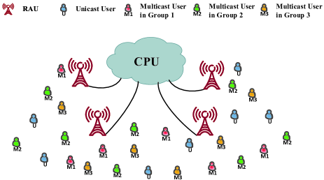
Figure 1: Joint unicast and multicast in cell-free distributed massive MIMO systems.

II-A System Configuration

We assume $N$ RAUs with $L$ antennas on each RAU, $U$ unicast users and $M$ multicast groups, among which the $m$-th multicast group contains $K_{\mathrm{m}}$ multicast users, and all users and RAUs are randomly distributed in the cell-free scenario. Fig. 1 presents such a system. During the joint unicast and multigroup multicast transmission, there are also downlink interferences affect the performance of the system.

II-B Channel Model

Considering frequency-flat fading channel, the channel vector between all RAUs and the $u$-th unicast user or the $k$-th multicast user in $m$-th multicast group can be described as

$$\mathbf{c}_{u} ={\mathbf{\beta}_{u}^{1/2}\mathbf{h}_{u}}{{\in{\mathbb{C}}^{NL\times 1}}},$$ (1)

$$\mathbf{t}_{m,k} ={\mathbf{\eta}_{m,k}^{1/2}\mathbf{h}_{m,k}}{{\in{\mathbb{C}}^{NL\times 1}}},$$ (2)

where ${{\mathbf{\beta}}_{u}}=\mathbb{E}\left[\mathbf{c}_{u}\mathbf{c}_{u}^{\mathrm{H}}\right]=\text{diag}\left(\left[{{\beta}_{1,u}},...,{{\beta}_{N,u}}\right]\right)\otimes{{\mathbf{I}}_{L}}$ and ${{\mathbf{\eta}}_{m,k}}=\mathbb{E}\left[\mathbf{t}_{m,k}\mathbf{t}_{m,k}^{\mathrm{H}}\right]=\text{diag}\left(\left[{{{\eta}_{1,m,k}},...,}{{{\eta}_{N,m,k}}}\right]\right)\otimes{{\mathbf{I}}_{L}}$ refer to the channel covariance matrix, ${{\mathbf{\beta}}_{n,u}}$ and ${{\eta}_{n,m,k}}$ represent the large-scale fading between the $n$-th RAU and the $u$-th unicast user or the $k$-th multicast user in the $m$-th multicast group, ${{\mathbf{h}}_{u}}\sim\mathcal{C}\mathcal{N}(0,{{\mathbf{I}}_{NL}})$ and ${{\mathbf{h}}_{m,k}}\sim\mathcal{C}\mathcal{N}(0,{{\mathbf{I}}_{NL}})$ are the small-scale fast fading. It is assumed that the channels of different users are uncorrelated.

II-C Channel Estimation

The system adopts time division duplex (TDD) mode. Due to the reciprocity between uplink and downlink channels, the CSI obtained by uplink channel estimation can be used for the precoding of downlink data transmission. The system uses uplink pilot sequences sent by users for channel estimation. Since all the user terminals within a multicast group need the same data, they are combined to share one pilot signal, thus only $M+U$ pilot signals need to be transmitted, which greatly alleviates the pilot tension caused by the large number of multicast users.

The uplink received pilot signal at CPU can be written as

$$\mathbf{Y}= \sum\limits_{u=1}^{U}{\sqrt{\tau p_{\mathrm{ul},u}}{{\mathbf{c}}_{u}}\mathbf{\phi}_{\mathrm{pu},u}^{\mathrm{H}}}$$

$$+\sum\limits_{m=1}^{M}{\sum\limits_{k=1}^{{{K}_{m}}}{\sqrt{\tau{q}_{\mathrm{ul},m,k}}{{\mathbf{t}}_{m,k}}\mathbf{\phi}_{\mathrm{pm},m}^{\mathrm{H}}}}+\mathbf{N},$$ (3)

where $p_{\mathrm{ul},u}$ and ${q}_{\mathrm{ul},m,k}$ denote the uplink transmitted power of the $u$-th unicast user and the $k$-th multicast user in the $m$-th multicast group. ${{\mathbf{\phi}}_{\mathrm{pu},u}}$ and ${{\mathbf{\phi}}_{\mathrm{pm},m}}$ represent the orthogonal pilot sequences of the $u$-th unicast user and the $m$-th multicast group with length $\tau$. The length of pilot sequences $\tau$ need to satisfy $\left(M+U\right)\leq\tau\leq T$. To achieve lower pilot cost, $\tau$ can be chosen as $\tau=M+U$. $\mathbf{N}$ is a $NL\times\tau$ dimension complex additive white Gaussian noise (AWGN).

The linear MMSE estimation[37] of ${\mathbf{{f}}}_{u}$ can be given by

$${{\mathbf{\hat{c}}}_{u}}= \frac{\sqrt{\tau p_{\mathrm{ul},u}}{{\mathbf{\beta}}_{u}}}{\tau p_{\mathrm{ul},u}{{\mathbf{\beta}}_{u}}+\sigma_{\mathrm{ul}}^{2}{{\mathbf{I}}_{NL}}}\left(\sqrt{\tau p_{\mathrm{ul},u}}{{\mathbf{c}}_{u}}+{{\mathbf{n}}_{u}}\right)$$

$$= \mathbf{\lambda}_{u}^{{1}/{2}\;}{{\mathbf{\hat{h}}}_{u}},$$ (4)

where ${{\mathbf{\lambda}}_{u}}=\text{diag}([{{\lambda}_{1,u}},{{\lambda}_{2,u}},...,{{\lambda}_{N,u}}])\otimes{\mathbf{I}_{L}}$ is the equivalent large-scale fading, ${{\lambda}_{\mathrm{n,u}}}=\frac{\tau p_{\mathrm{ul},u}{{\beta}_{n,u}}^{2}}{\tau p_{\mathrm{ul},u}{{\beta}_{n,u}}+\sigma_{\mathrm{ul}}^{2}}$ and ${{\mathbf{\hat{h}}}_{u}}\sim\mathcal{C}\mathcal{N}(0,{{\mathbf{I}}_{NL}})$ is the equivalent small-scale fast fading.

Similarly, the linear MMSE estimation of ${\mathbf{t}}_{m,k}$ can be given by

$${{\mathbf{\hat{t}}}_{m,k}}=\mathbf{\xi}_{m,k}^{{1}/{2}\;}{{\mathbf{\hat{h}}}_{m,k}},$$ (5)

where ${{\mathbf{\xi}}_{m,k}}=\text{diag}\left(\left[{{\xi}_{1,m,k}},...,{{\xi}_{N,m,k}}\right]\right)\otimes{{\mathbf{I}}_{L}}$ is the equivalent large-scale fading, ${{\mathbf{\xi}}_{n,m,k}}=\frac{\tau{q}_{\mathrm{ul},m,k}\eta_{n,m,k}^{2}}{\sigma_{\mathrm{ul}}^{2}+\sum\nolimits_{j=1}^{{{K}_{m}}}{\tau{q}_{\mathrm{ul},m,j}{{\eta}_{n,m,j}}}}$ and ${{\mathbf{\hat{h}}}_{m,k}}\sim\mathcal{C}\mathcal{N}(0,{{\mathbf{I}}_{NL}})$.

By adopting co-pilot strategy, we can obtain the equivalent channel state information of the multicast group [27]. Compared with the case of fully orthogonal pilots, this method greatly saves pilot overhead. In addition, the same multicast group requires the same information to be transmitted, so the error due to pilot multiplexing is small. To reduce pilot cost, we design a unified precoding for each multicast group. The co-pilot assignment strategy based channel estimation of multicast groups $\mathbf{{t}}_{m}=\sum\nolimits_{j=1}^{{{K}_{m}}}{\sqrt{\tau{q}_{\mathrm{ul},m,j}}}{{\mathbf{t}}_{m,j}}$ is adopted and the closed-form expression can be given by

$${{\mathbf{\hat{t}}}_{m}}= \frac{\sum\nolimits_{j=1}^{{{K}_{m}}}{\tau{q}_{\mathrm{ul},m,j}{{\mathbf{\eta}}_{m,j}}}\left(\sum\nolimits_{j=1}^{{{K}_{m}}}{\sqrt{\tau{q}_{\mathrm{ul},m,j}}{{\mathbf{t}}_{m,j}}}+{{\mathbf{n}}_{m}}\right)}{\sum\nolimits_{j=1}^{{{K}_{m}}}{\tau{q}_{\mathrm{ul},m,j}{{\mathbf{\eta}}_{m,j}}}+\sigma_{\mathrm{ul}}^{2}{{\mathbf{I}}_{NL}}}$$

$$= \mathbf{\mu}_{m}^{{1}/{2}\;}{{\mathbf{\hat{h}}^{*}}_{m}},$$ (6)

where ${{\mathbf{\mu}}_{m}}=\text{diag}\left(\left[{{\mu}_{1,m}},{{\mu}_{2,m}},...,{{\mu}_{N,m}}\right]\right)\otimes{{\mathbf{I}}_{L}}$ is the equivalent large-scale fading, ${{\mu}_{n,m}}=\frac{{{(\sum\nolimits_{j=1}^{{{K}_{m}}}{\tau{q}_{\mathrm{ul},m,j}{{\eta}_{n,m,j}}})}^{2}}}{\sum\nolimits_{j=1}^{{{K}_{m}}}{\tau{q}_{\mathrm{ul},m,k}{{\eta}_{n,m,j}}}+\sigma_{\mathrm{ul}}^{2}}$ and ${{\mathbf{\hat{h}}^{*}}_{m}}\sim\mathcal{C}\mathcal{N}(0,{{\mathbf{I}}_{NL}})$.

Remark 1

As seen from (5) and (II-C), the channel estimation of multicast group $m$ can be given by ${{\mathbf{\hat{t}}}_{m}}=\sum\nolimits_{j=1}^{{{K}_{m}}}{\sqrt{\tau{q}_{\mathrm{ul},m,j}}}{{\mathbf{\hat{t}}}_{m,j}}$ which is a linear combination of the channel estimations of all users within the $m$-th multicast group. Under the traditional orthogonal pilot estimation scheme, each user in the multicast group need to be assigned orthogonal pilots as unicast and the pilot overhead will be extremely large. As a result, the channel estimation of multigroup multicast (II-C) and unicast (II-C) are completed respectively to save pilot cost and increase accuracy simultaneously.

III Downlink Data Transmission

In this section, the downlink transmission of joint unicast and multigroup multicast in cell-free distributed massive MIMO is studied. Since the transmission expressions of multicast and unicast are relatively similar, only the expression of multigroup multicast in joint unicast and multigroup multicast transmission is given below.

The received signal of the $k$-th multicast user terminal in the $m$-th multicast group can be presented as:

$${{z}_{m,k}}= \mathbf{t}_{m,k}^{\mathrm{H}}(\mathbf{Wx}+\mathbf{Vs})+{{n}_{m,k}}$$

$$= \mathbf{t}_{m,k}^{\mathrm{H}}{{\mathbf{w}}_{m}}{{x}_{m}}+\sum\limits_{r=1,r\neq m}^{M}{\mathbf{t}_{m,k}^{\mathrm{H}}{{\mathbf{w}}_{r}}{{x}_{r}}}$$

$$+\sum\limits_{u=1}^{U}{\mathbf{t}_{m,k}^{\mathrm{H}}{{\mathbf{v}}_{u}}{{s}_{u}}}+{{n}_{m,k}},$$ (7)

where ${{n}_{m,k}}\sim\mathcal{C}\mathcal{N}(0,\sigma_{\mathrm{dl}}^{2})$ are complex AWGN vectors, $\mathbf{x}={{\left[{{x}_{1}},...,{{x}_{M}}\right]}^{\text{T}}}$ and $\mathbf{s}=\left[{{s}_{1}},...,{{s}_{U}}\right]{}^{\mathrm{T}}$ are the data transmitted to multicast groups and unicast users. $\mathbf{W}={{[{{\mathbf{w}}_{1}},{{\mathbf{w}}_{2}},...,{{\mathbf{w}}_{M}}]}^{\mathrm{T}}}$ and $\mathbf{V}={{[{{\mathbf{v}}_{1}},{{\mathbf{v}}_{2}},...,{{\mathbf{v}}_{U}}]}^{\mathrm{T}}}$ are the precoding matrixes of multicast groups and unicast users.

III-A Downlink Channel Precoding

To facilitate the comparison of the performance under different precoding schemes, we use the average power normalization criterion [38, 39] to design the precoding vectors. The precoding for each multicast group can be given by

$$\mathbf{w}_{m}^{\mathrm{pre}}{=}\frac{\sqrt{q_{\mathrm{dl},m}}\mathbf{\hat{a}}{{}_{m}^{\mathrm{pre}}}}{\mathbb{E}{{\left[\left(\mathbf{\hat{a}}{{}_{m}^{\mathrm{pre}}}\right)^{\mathrm{H}}\mathbf{\hat{a}}{{}_{m}^{\mathrm{pre}}}\right]}^{1/2}}},$$ (8)

where $\mathrm{pre}\in\left\{\mathrm{MRT,ZF,MMSE}\right\}$, $q_{\mathrm{dl},m}$ are the downlink power of multicast precoding vectors and $\mathbb{E}\left[{{\left\|\mathbf{w}_{m}^{\mathrm{pre}}\right\|}^{2}}\right]={q}_{\mathrm{dl},m}$. By replacing the corresponding items with unicast, the unicast precoding vector $\mathbf{v}_{u}^{\mathrm{pre}}$ can be obtained.

The item ${\mathbb{E}{{\left[\left(\mathbf{\hat{a}}{{}_{m}^{\mathrm{pre}}}\right)^{\mathrm{H}}\mathbf{\hat{a}}{{}_{m}^{\mathrm{pre}}}\right]}}}$ in (8) needs further calculation. For MRT precoding, we have $\mathbf{\hat{a}}{{}_{m}^{\mathrm{MRT}}}={{\mathbf{\hat{t}}}_{m}}$,

$$\mathbb{E}{{\left[\left(\mathbf{\hat{a}}{{}_{m}^{\mathrm{MRT}}}\right)^{\mathrm{H}}\mathbf{\hat{a}}{{}_{m}^{\mathrm{MRT}}}\right]}}= L\sum\limits_{n=1}^{N}{\frac{{{(\sum\nolimits_{j=1}^{{{K}_{m}}}{\tau q_{\mathrm{ul},m,j}{{\eta}_{n,m,j}}})}^{2}}}{{\sum\nolimits_{j=1}^{{{K}_{m}}}{\tau q_{\mathrm{ul},m,j}{{\eta}_{n,m,j}}}}+\sigma_{\mathrm{ul}}^{2}}}$$

$$= L\sum\limits_{n=1}^{N}{{{\mu}_{n,m}}}.$$ (9)

With the definition of ${\upsilon}_{m}=\sum_{n=1}^{N}{{{\mu}_{n,m}}}$, we have

$$\mathbf{w}_{m}^{\mathrm{MRT}}=\sqrt{\frac{q_{\mathrm{dl},m}}{L{{\upsilon}_{m}}}}{{\mathbf{\hat{t}}}_{m}}.$$ (10)

For ZF precoding, we have $\mathbf{\hat{a}}{{}_{m}^{\mathrm{ZF}}}=\left[\mathbf{\hat{Q}(}{{\mathbf{\hat{Q}}}^{\mathrm{H}}}\mathbf{\hat{Q}}{{\mathbf{)}}^{\mathbf{-1}}}\right]_{U+m}$, where $\mathbf{\hat{Q}}=\left[\mathbf{\hat{C},\hat{T}}\right]$, $\mathbf{\hat{C}}=\left[{{{\mathbf{\hat{c}}}}_{1}},{{{\mathbf{\hat{c}}}}_{2}},...,{{{\mathbf{\hat{c}}}}_{U}}\right]$, $\mathbf{\hat{T}}=\left[{{{\mathbf{\hat{t}}}}_{1}},{{{\mathbf{\hat{t}}}}_{2}},...,{{{\mathbf{\hat{t}}}}_{M}}\right]$, $\left[\cdot\right]_{i}$ represents the $i$-th column of the matrix,

$$\mathbb{E}{{\left[\left(\mathbf{\hat{a}}{{}_{m}^{\mathrm{ZF}}}\right)^{\mathrm{H}}\mathbf{\hat{a}}{{}_{m}^{\mathrm{ZF}}}\right]}}= \mathrm{tr}\left(\mathbf{\hat{Q}}^{\mathrm{H}}\left({{\left({\mathop{{{{\mathbf{\hat{Q}}}}^{\mathrm{H}}}\mathbf{\hat{Q}}}}\right)}^{-1}}\right)^{\mathrm{H}}\times{{\left({\mathop{{{{\mathbf{\hat{Q}}}}^{\mathrm{H}}}\mathbf{\hat{Q}}}}\right)}^{-1}}\mathbf{\hat{Q}}\right)$$

$$= {{((NL-M-U){{\upsilon}_{m}})}^{\text{-2}}}\mathrm{tr}\left(\mathbf{\hat{Q}}^{\mathrm{H}}\mathbf{\hat{Q}}\right)$$

$$= {({(NL-M-U){{\upsilon}_{m}}})^{-1}},$$ (11)

and the precoding vector can be given by

$$\mathbf{w}_{m}^{\mathrm{ZF}} =\sqrt{Aq_{\mathrm{dl},m}{{\upsilon}_{m}}}\left[\mathbf{\hat{Q}(}{{{\mathbf{\hat{Q}}}}^{\mathrm{H}}}\mathbf{\hat{Q}}{{\mathbf{)}}^{\mathbf{-1}}}\right]_{U+m},$$ (12)

where $A=NL-M-U$.

For MMSE precoding, with the estimated vector $\mathbf{\hat{a}}{{}_{m}^{\mathrm{MMSE}}}=\left[\mathbf{\hat{Q}}{{\left({\mathop{{{{\mathbf{\hat{Q}}}}^{\mathrm{H}}}\mathbf{\hat{Q}}+\sigma_{\mathrm{dl}}^{2}}}\,\otimes{\mathbf{I}_{NL}}\right)}^{-1}}\right]_{U+m}$, the pending item can be given by

$$\mathbb{E}{{\left[\left(\mathbf{\hat{a}}{{}_{m}^{\mathrm{MMSE}}}\right)^{\mathrm{H}}\mathbf{\hat{a}}{{}_{m}^{\mathrm{MMSE}}}\right]}}$$

$$= \mathrm{tr}\Big{(}\begin{aligned} &\mathbf{\hat{Q}}^{\mathrm{H}}\left({{\left({\mathop{{{{\mathbf{\hat{Q}}}}^{\mathrm{H}}}\mathbf{\hat{Q}}+\sigma_{\mathrm{dl}}^{2}}}\,\otimes{\mathbf{I}_{NL}}\right)}^{-1}}\right)^{\mathrm{H}}\\ &\times{{\left({\mathop{{{{\mathbf{\hat{Q}}}}^{\mathrm{H}}}\mathbf{\hat{Q}}+\sigma_{\mathrm{dl}}^{2}}}\,\otimes{\mathbf{I}_{NL}}\right)}^{-1}}\mathbf{\hat{Q}}\end{aligned}\Big{)}$$

$$= {{(A{{\upsilon}_{m}}+\sigma_{\mathrm{dl}}^{2})}^{\text{-2}}}\mathrm{tr}\left(\mathbf{\hat{Q}}^{\mathrm{H}}\mathbf{\hat{Q}}\right)$$

$$= {{{(A{{\upsilon}_{m}}+\sigma_{\mathrm{dl}}^{2})}^{\text{-2}}}A{\upsilon}_{m}},$$ (13)

and the precoding vector can be given by

$$\mathbf{w}_{m}^{\mathrm{MMSE}}$$

$$= \sqrt{\frac{q_{\mathrm{dl},m}{{\left(A{{\upsilon}_{m}}+\sigma_{\text{dl}}^{2}\right)}^{2}}}{A{{\upsilon}_{m}}}}\left[\mathbf{\hat{Q}}{{\left({\mathop{{{{\mathbf{\hat{Q}}}}^{\mathrm{H}}}\mathbf{\hat{Q}}+\sigma_{\mathrm{dl}}^{2}}}\otimes{\mathbf{I}_{NL}}\right)}^{-1}}\right]_{U+m}.$$ (14)

The corresponding precoding vectors of unicast $\mathbf{v}_{u}^{\mathrm{pre}}$ can be obtained by replacing $q_{\mathrm{dl},m}$ and ${{\upsilon}_{m}}$ with the downlink power of unicast precoding vectors $p_{\mathrm{dl},u}$ and the estimated covariance matrix of unicast ${{\theta}_{u}}=\sum_{n=1}^{N}{\frac{\tau p_{\mathrm{ul},u}{{\beta}_{n,u}^{2}}}{\tau p_{\mathrm{ul},u}{{\beta}_{n,u}}+\sigma_{\mathrm{ul}}^{2}}}$ and $\mathbb{E}\left[{{\left\|\mathbf{v}_{u}^{\mathrm{pre}}\right\|}^{2}}\right]=p_{\mathrm{dl},u}$.

Remark 2

Different from pure unicast or multicast, the joint unicast and multicast transmission system not only retains the individualization of unicast, but also promotes the efficiency of transmitting repeated information by multicast.

IV Spectral Efficiency Analysis

In this section, we analyze the downlink achievable SE of user terminals with different precoding schemes in joint unicast and multigroup multicast transmission systems under cell-free distributed massive MIMO scenarios. According to the standard capacity bounding technique in [32, 40, 8], the received signal from the RAUs to the $k$-th unicast user and the $k$-th multicast user in the $m$-th multicast group can be rewritten as

$${{y}_{k}}= \mathbb{E}\left[\mathbf{c}_{k}^{\mathrm{H}}{{\mathbf{v}}_{k}}\right]{{s}_{k}}+\left(\mathbf{c}_{k}^{\mathrm{H}}{{\mathbf{v}}_{k}}-\mathbb{E}\left[\mathbf{c}_{k}^{\mathrm{H}}{{\mathbf{v}}_{k}}\right]\right){{s}_{k}}$$

$$+\sum\limits_{u=1,u\neq k}^{U}{\mathbf{c}_{k}^{\mathrm{H}}{{\mathbf{v}}_{u}}{{s}_{u}}}+\sum\limits_{r=1}^{M}{\mathbf{c}_{k}^{\mathrm{H}}{{\mathbf{w}}_{r}}{{x}_{r}}}+{{n}_{k}},$$ (15)

$${z}_{m,k}= \mathbb{E}\left[\mathbf{t}_{m,k}^{\mathrm{H}}{{\mathbf{w}}_{m}}\right]{{x}_{m}}+\left(\mathbf{t}_{m,k}^{\mathrm{H}}{{\mathbf{w}}_{m}}-\mathbb{E}\left[\mathbf{t}_{m,k}^{\mathrm{H}}{{\mathbf{w}}_{m}}\right]\right){{x}_{m}}$$

$$+\sum\limits_{r=1,r\neq m}^{M}{\mathbf{t}_{m,k}^{\mathrm{H}}{{\mathbf{w}}_{r}}{{x}_{r}}}+\sum\limits_{u=1}^{U}{\mathbf{t}_{m,k}^{\text{H}}{{\mathbf{v}}_{u}}{{s}_{u}}}+{{n}_{m,k}},$$ (16)

where $\mathbb{E}\left[\mathbf{c}_{k}^{\mathrm{H}}{{\mathbf{v}}_{k}}\right]{{s}_{k}}$, $\mathbb{E}\left[\mathbf{t}_{m,k}^{\mathrm{H}}{{\mathbf{w}}_{m}}\right]{{x}_{m}}$ can be regarded as the signals needed and the others are interferences and noises.

In terms of [4], the achievable SE can be given by

$$\text{SE}^{\mathrm{pre}}=\left(1-\frac{\tau}{T}\right){{\log}_{2}}\left(1+\text{SINR}^{\mathrm{pre}}\right),$$ (17)

where the SINR of unicast and multicast can be represented as (18) and (19).

$$\text{SINR}_{k,un}^{\mathrm{pre}} =\frac{{{\left|\mathbb{E}\left[\mathbf{c}_{k}^{\mathrm{H}}\mathbf{v}_{k}^{\mathrm{pre}}\right]\right|}^{2}}}{\sigma_{\mathrm{dl}}^{2}-{{\left|\mathbb{E}\left[\mathbf{c}_{k}^{\mathrm{H}}\mathbf{v}_{k}^{\mathrm{pre}}\right]\right|}^{2}}+\sum\limits_{u=1}^{U}{\mathbb{E}\left[{{\left|\mathbf{c}_{k}^{\mathrm{H}}\mathbf{v}_{u}^{\mathrm{pre}}\right|}^{2}}\right]}+\sum\limits_{r=1}^{M}{\mathbb{E}\left[{{\left|\mathbf{c}_{k}^{\mathrm{H}}\mathbf{w}_{r}^{\mathrm{pre}}\right|}^{2}}\right]}},$$ (18)

$$\text{SINR}_{m,k,mu}^{\mathrm{pre}} =\frac{{{\left|\mathbb{E}\left[\mathbf{t}_{m,k}^{\text{H}}\mathbf{w}_{m}^{\text{pre}}\right]\right|}^{2}}}{\sigma_{\mathrm{dl}}^{2}-{{\left|\mathbb{E}\left[\mathbf{t}_{m,k}^{\text{H}}\mathbf{w}_{m}^{\text{pre}}\right]\right|}^{2}}+\sum\limits_{u=1}^{U}{\mathbb{E}\left[{{\left|\mathbf{t}_{m,k}^{\text{H}}\mathbf{v}_{u}^{\text{pre}}\right|}^{2}}\right]}+\sum\limits_{r=1}^{M}{\mathbb{E}\left[{{\left|\mathbf{t}_{m,k}^{\text{H}}\mathbf{w}_{r}^{\text{pre}}\right|}^{2}}\right]}},$$ (19)

$$\text{SINR}_{k,un}^{\text{pre}} =\frac{Jp_{\text{dl},k}{{\theta}_{k}}}{\sigma_{\text{dl}}^{2}+\sum\limits_{u=1}^{U}\left[\frac{1}{NL}{p_{\text{dl},u}\sum\limits_{n=1}^{N}{{\beta}_{n,k}}}\right]+\sum\limits_{r=1}^{M}{\left[\frac{1}{NL}q_{\mathrm{dl},r}\sum\limits_{n=1}^{N}{{{\beta}_{n,k}}}\right]}},$$ (20)

$$\text{SINR}_{m,k,mu}^{\mathrm{pre}} =\frac{Jq_{\mathrm{dl},m}{{\zeta}_{m,k}}}{\sigma_{\mathrm{dl}}^{2}+\sum\limits_{u=1}^{U}{\left[\frac{1}{NL}p_{\mathrm{dl},u}\sum\limits_{n=1}^{N}{{{\eta}_{n,m,k}}}\right]}+\sum\limits_{r=1}^{M}{\left[\frac{1}{NL}q_{\mathrm{dl},r}\sum\limits_{n=1}^{N}{\eta_{n,m,k}}\right]}},$$ (21)

 

Theorem 1

Each item can be solved with different precoding schemes obtained in the previous section and the closed-form expressions of achievable SINR with different precoding can be given by (20) and (21), where ${{\zeta}_{m,k}}=\sum_{n=1}^{N}{\frac{\tau q_{\mathrm{ul},m,k}\eta_{n,m,k}^{2}}{\sigma_{\mathrm{ul}}^{2}+\sum\nolimits_{j=1}^{{{K}_{m}}}{\tau q_{\mathrm{ul},m,j}{{\eta}_{n,m,j}}}}}$,

$$J=\left\{\begin{aligned} &L,\quad\quad\quad\quad\quad\quad\quad\quad\quad\quad\,\,\,\,\text{for MRT},\\ &NL-M-U,\quad\quad\quad\quad\quad\,\,\,\text{for ZF},\\ &{{\left(NL\right)}^{2}}/\left(NL-M-U\right),\quad\text{for MMSE}.\end{aligned}\right.$$

Proof: Please refer to Appendix A.

Remark 3

In cell free distributed massive MIMO scenarios, due to the operation between RAUs, the SE of unicast and multicast can be greatly promoted and since the closed-form expressions we derived only rely on large-scale fading parameters which change much slower than small-scale parameters, this is much highly practical. The complex formulas in distributed scenario can be transformed into simpler forms in centralized scenarios by setting the number of RAUs $N=1$ while the formulas for centralized scenarios cannot be easily applied to distributed scenarios.

V Joint Spectral Efficiency Optimization

The derived closed-form expression of achievable SE (also SINR) shows that SE can be influenced by downlink transmitted power, uplink pilot power and length of the pilot sequence $\tau$ . To achieve higher SE, the allocation of these resources needs to be considered, subject to various constraints. For multicast, a problem worth studying is the MMF, in which the minimum SINR or SE of the system needs to be maximized with a limited transmitted power. However, due to the interference between unicast and multicast, the SE of multicast and unicast users are conflicting with each other, i.e. with the increase of the downlink power of multicast, the SE of unicast users will decrease and vice versa, which means that multicast and unicast users can not achieve the highest SE simultaneously. Therefore, a multi-objective optimization problem(MOOP) is formulated. One objective is the average achievable SE of unicast users and the other one is the MMF problem for multicast users. Finally, we solve this MOOP problem with NSGA-II.

V-A Problem Formulation

For multicast, the MMF problem can be described as

$$\underset{\mathcal{P},\tau}{\mathop{\text{missing}}{max}}\quad{f1}= \min\,\,\,\text{SE}_{m,k,mu}^{\text{pre}}$$ (22)

$${\rm{s}}{\rm{.t}}{\rm{.}}\quad C1: \text{SE}_{m,k,mu}^{\text{pre}}\geq\text{SE}_{m,k,mu}^{\text{pre,min}},\,\forall m\in\mathcal{M},\forall k\in{\mathcal{K}_{m}},$$

$$\text{SE}_{k,un}^{\text{pre}}\geq\text{SE}_{k,un}^{\text{pre,min}},\forall u\in\mathcal{U},$$ (23)

$$C2: {{p}_{\mathrm{ul},k}}\leq{{P}_{\mathrm{ul},un}},\forall u\in\mathcal{U},\,\,\,$$

$${{q}_{\mathrm{ul},m,k}}\leq{{P}_{\mathrm{ul},mu}},\forall m\in\mathcal{M},\forall k\in{\mathcal{K}_{m}},$$ (24)

$$C3: \sum_{k=1}^{U}{{{p}_{\mathrm{dl},k}}}\leq{{P}_{\mathrm{dl},un}},\,\sum_{m\text{=}1}^{M}{{{q}_{\mathrm{dl},m}}}\leq{{P}_{\mathrm{dl},mu}},$$ (25)

$$\sum_{k=1}^{U}{{{p}_{\mathrm{dl},k}}}+\sum_{m\text{=}1}^{M}{{{q}_{\mathrm{dl},m}}}\leq{{P}_{\mathrm{dl}}},$$ (26)

$$C4: {{p}_{\mathrm{ul},k}}\geq 0,{{q}_{\mathrm{ul},m,k}}\geq 0,{{p}_{\mathrm{dl},k}}\geq 0,{{q}_{\mathrm{dl},m}}\geq 0,$$ (27)

$$C5: \tau\in\left\{M+U,...,T\right\},$$ (28)

where $\mathcal{P}=\left\{{{\text{p}}_{\text{ul}}}\text{,}{{\text{q}}_{\text{ul}}}\text{,}{{\text{p}}_{\text{dl}}}\text{,}{{\text{q}}_{\text{dl}}}\right\}$, ${{\text{p}}_{\text{ul}}}=\left[{{p}_{\mathrm{ul},1}},\cdots,{{p}_{\mathrm{ul},U}}\right]$, ${{\text{p}}_{\text{dl}}}=\left[{{p}_{\mathrm{dl},1}},\cdots,{{p}_{\mathrm{dl},U}}\right]$, ${{\text{q}}_{\text{dl}}}=\left[{{q}_{\mathrm{dl},1}},\cdots,{{q}_{\mathrm{dl},M}}\right]$, ${{\text{q}}_{\text{ul}}}=\left[{{q}_{\mathrm{ul},1,1}},\cdots,{{q}_{\mathrm{ul},1,{{K}_{1}}}};\cdots;{{q}_{\mathrm{ul},M,1}},\cdots,{{q}_{\mathrm{ul},M,{{K}_{M}}}}\right]$. $C1$ are the ergodic downlink QoS constraints where $\text{SE}_{m,k,mu}^{\text{pre,min}}>0$ and $\text{SE}_{k,un}^{\text{pre,min}}>0$ are the required minimum SE of multicast and unicast users. $C2$ are the uplink power constraints where ${{P}_{\mathrm{ul},un}}$ and ${{P}_{\mathrm{ul},mu}}$ are the upper limits of the uplink transmitted power per user of unicast and multicast. $C3$ are the total downlink power constraints of all RAUs where ${{P}_{\mathrm{dl},un}}$ and ${{P}_{\mathrm{dl},mu}}$ are the upper limits of total downlink transmitted power of unicast and multicast and ${{P}_{\mathrm{dl}}}$ is the total downlink power threshold. According to the discussion about the pilot sequence length in Section II, we can give the optimal value of $C5$ is $\tau^{*}=M+U$. Due to the non-convexity of $\text{SE}_{m,k,mu}^{\text{pre}}$, it is very difficult to find the maximum value.

For unicast, the average SE optimization problem can be formulated as

$$\underset{\mathcal{P},\tau}{\mathop{\text{missing}}{max}}\quad\, {f2}=\sum\limits_{u=1}^{U}{\text{SE}_{u,un}^{\text{pre}}}/U,$$ (29)

$${\rm{s}}{\rm{.t}}{\rm{.}}\quad\,\, C1-C5.$$ (30)

The MMF problem of multicast $\mathop{f1}$ and the maximization of average achievable SE of unicast $\mathop{f2}$ are conflicting. Thus we propose a MOOP to investigate the trade-off between these two problems

$$\underset{\mathcal{P},\tau}{\mathop{\text{missing}}{max}}\,\,\quad \mathbf{F}{=}{{\left[f1,f2\right]}^{\text{T}}},$$ (31)

$${\rm{s}}{\rm{.t}}{\rm{.}}\quad\,\, C1-C5,$$ (32)

where $\mathbf{F}$ is the optimal vector containing the objective functions $f1$ and $f2$. The MOOP aims to maximize the minimum SE of multicast and the average SE of unicast simultaneously.

V-B Solutions by Multi-objective Genetic Algorithm

Most optimization methods transform a MOOP into multiple single-objective optimizations by giving one Pareto-optimal solution at a run. However, these kinds of methods may obtain different solutions at different runs and not give a joint optimal solution. $f1$ and $f2$ are both non-convex problems due to the non-convexity of $\text{SE}_{m,k,mu}^{\text{pre}}$ and $\text{SE}_{u,un}^{\text{pre}}$ . In order to solve the two objectives simultaneously in a single simulation run, the multi-objective evolutionary algorithms (MOEAs) is utilized to obtain the Pareto boundary of (31). Therefore, we adopt MOEAs to obtain the simultaneous Pareto-optimal solutions in this paper. Specifically, NSGA-II [41] which has been proved to be reliable and effective in [42] is utilized to solve the proposed MOOP.

NSGA-II is an elitist nondominated sorting genetic algorithm with a lower complexity of $O(XY^{2})$, where $X$ is the number of objective functions and $Y$ is the population size. According to NSGA-II, firstly, an initial population with a size of $Y$ is randomly generated. In our case, the uplink pilot power, the downlink transmitted power and the coherence time are selected under the constraints given in (25) - (28). Secondly, the two objective functions are evaluated based on the current population by calculating the minimum SE of multicast users and the average SE of unicast users as (22) and (29). Thirdly, we rank the population based on fast non-dominated sorting and crowdedness. Then a new parent population is selected from the currently ranked population by tournament selection and an offspring population is generated by selection, mutation, and crossing. Finally, the offspring population and initial population are combined together and ranked to a new initial population. The cycle repeats until the optimization criteria are met and the Pareto boundary of the MOOP can be found. The power allocation algorithm based on NSGA-II is shown in Algorithm 1.

Algorithm 1 Power Allocation Algorithm Based on NSGA-II

  Initialization:

• initialize system parameters: the uplink transmitted power of unicast and mulicast ${{\text{p}}_{\text{ul}}}$, ${{\text{q}}_{\text{ul}}}$, the downlink transmitted power of unicast and mulicast ${{\text{p}}_{\text{dl}}}$, ${{\text{q}}_{\text{dl}}}$, the size of population $Y$ and so on

• generate the population randomly under the constraints given in (25) - (28)

  Evaluation:

• evaluate the two objective functions: the minimum SE of multicast users and the average SE of unicast users as (22) and (29)

• select an excellent parent population to generate offspring population by selection, mutation, and crossing

  Sort:

• rank each individual based on non-dominating sorting and crowding distance

  Repeat:

• select an excellent parent population to generate offspring population by selection, mutation, and crossing

• rank the $2Y$ combined offspring population and the old population to generate a new population

  Until the stop criterion of optimization

  Return a series of Pareto optimal solutions of (31)

VI Unsupervised Deep Learning Based Power Allocation

Given the proposed MOOP in (31), to further reduce the computational complexity, we introduce an unsupervised DL method to optimize the achievable rate of multicast and unicast users and compare it with NSGA-II algorithm.

VI-A Network Design

The traditional DL approach is to decrease the loss function continuously and minimize the loss function [43, 44]. To meet the demands of maximizing the average SE of unicast and the minimum SE of multicast users, we take the negative SE as the loss function, so while the loss function is decreasing, the SE is increasing. The loss function can be given by

$$\underset{\mathcal{P}}{loss}= \mathbb{E}\left[los{{s}_{ase}}+los{{s}_{mmf}}\right]$$

$$= \mathbb{E}\left[-\sum\limits_{u=1}^{U}{\text{SE}_{k,un}^{\text{pre}}}/U-\min\left(\text{SE}_{m,k,mu}^{\text{pre}}\right)\right].$$ (33)

Through the optimization of the coherence time $T$ with NSGA-II, we can obtain the approximately optimal value $T^{*}$ and the loss function can be given by

$$\underset{\mathcal{P}}{loss}$$

$$= \mathbb{E}\Big{[}\left(1-\frac{M+U}{{{T}^{*}}}\right)\Big{(}\begin{aligned} &-\sum_{u=1}^{U}{{{\log}_{2}}\left(1+\text{SINR}_{k,un}^{\text{pre}}\right)}/U\\ &-\min{{\log}_{2}}\left(1+\text{SINR}_{m,k,mu}^{\text{pre}}\right)\end{aligned}\Big{)}\Big{]}.$$ (34)

Since some of the optimization variables have been determined, the optimization problem can be transformed into maximizing the achievable rate and loss function

$$\underset{\mathcal{P}}{loss}^{{}^{\prime}}=\mathbb{E}\Big{[}\begin{aligned} &-\sum\limits_{u=1}^{U}{{{\log}_{2}}\left(1+\text{SINR}_{k,un}^{\text{pre}}\right)}/U\\ &-\min\left({{\log}_{2}}\left(1+\text{SINR}_{m,k,mu}^{\text{pre}}\right)\right)\end{aligned}\Big{]}.$$ (35)

VI-B Network Structure

In this part, we consider a fully connected deep neural network (DNN) to maximize the achievable rate of unicast and multicast users. The input of DNN are the channel large-scale fading of the system $\mathbf{\beta}_{u}$ and $\mathbf{\eta}_{m,k}$. The output of DNN is the power allocation strategy $\mathcal{P}$ to maximize the achievable SE, where the first $U+M$ outputs denote the optimal downlink transmitted power of unicast and multicast and the following outputs denote the optimal uplink pilot power. The DNN is trained to learn the nonlinear mapping between the large-scale fading and the power allocation scheme.

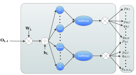
Figure 2: The detailed structure of the output layer of the unsupervised learning based DNN.

The detailed structure of the output layer is shown in Fig. 11, where ${{\mathbf{o}}_{L-1}}$ is the output of the hidden layer. ${{\mathbf{W}}_{L}}$ is the weight matrix and ${{\mathbf{b}}_{L}}$ is the bias vector of layer $L$, which needs to be optimized in neural networks. Processed by a linear transformation $\mathbf{g}={{\mathbf{W}}_{L}}{{\mathbf{o}}_{L-1}}+{{\mathbf{b}}_{L}}$, a temporary output $\mathbf{g}$ can be obtained. Then $\mathbf{g}=\left[g_{1},\cdots,{{g}_{K}}\right]$ is divided into two groups. One is from ${{g}_{1}}$ to ${{g}_{M+U}}$ and the other is from ${{g}_{M+U+1}}$ to ${{g}_{K}}$ where $K=2U+M+\sum_{m=1}^{M}{{{K}_{m}}}$. In order to achieve the power constraints proposed in (V-A) - (27), each group is first submitted to a Softmax function to achieve normalization and then multiplies the power constraints of the group, which can be expressed as

$${{p}_{k}}=\left\{\begin{aligned} &p_{\text{dl}}^{\text{tot}}\sigma\left({{g}_{k}}\right),\quad 1\leq k\leq M+U,\\ &p_{\text{ul}}^{\text{tot}}\sigma\left({{g}_{k}}\right),\quad M+U+1\leq k\leq K,\\ \end{aligned}\right.$$ (36)

where

$$\sigma\left({{t}_{k}}\right)=\left\{\begin{aligned} &\frac{{{e}^{{{t}_{k}}}}}{\sum\nolimits_{k=1}^{M+U}{{{e}^{{{t}_{k}}}}}},\quad\quad\,\,1\leq k\leq M+U,\\ &\frac{{{e}^{{{t}_{k}}}}}{\sum\nolimits_{k=M+U+1}^{K}{{{e}^{{{t}_{k}}}}}},\,\,M+U+1\leq k\leq K,\\ \end{aligned}\right.$$ (37)

and $p_{\text{dl}}^{\text{tot}}=\sum_{k=1}^{M+U}{{{p}_{k}}}$, $p_{\text{ul}}^{\text{tot}}=\sum_{k=M+U{+}1}^{K}{{{p}_{k}}}$ are the total power constraints of uplink and downlink.

We adopt the Adaptive Moment Estimation (Adam) algorithm for optimization, which is essentially an RMSprop algorithm with a momentum term. Adjusting the learning rate of each parameter, it can minimize the loss function and maximize the optimization objective. The main advantage of Adam is that after bias correction, each iteration of the learning rate has a certain range, which makes the parameters relatively stable.

The complexity of training phase can be regarded as $O\left(2\left(KN{{n}_{1}}+K\tau{{n}_{L-1}}+\sum\limits_{l=2}^{L-1}{{{n}_{l-1}}{{n}_{l}}}\right)st\right)$, where $s$ is the size of mini-batch, $t$ is the number of iterations and $n_{l}$ denotes the number of nodes of the $l$-th layer. Through the training of the DNN with the large-scale fading coefficients, the considered DL problem can be solved. Therefore, the complexity of solving the DL problem mainly depends on forward propagation, which can be given by $O\left(KN{{n}_{1}}+K\tau{{n}_{L-1}}+\sum\limits_{l=2}^{L-1}{{{n}_{l-1}}{{n}_{l}}}\right)$ and it indeed reduces the complexity than NSGA-II.

VII Numerical Results

In this section, we use Monte Carlo simulation to verify the closed-form expression derived. With the numerical result, we analyze the SE of unicast and multigroup multicast users under different precoding schemes.

VII-A Simulation Parameters

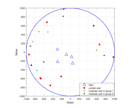
Figure 3: Simulation system configure.

TABLE I: Simulation parameter settings

Item	Number
Number of unicast users $U$	10
Number of multicast groups $M$	2
Number of multicast users in each group $K_{m}$	[5,5]
Path loss index $a$	3.7
Uplink power $p_{\mathrm{ul},u}$ and ${q}_{\mathrm{ul},m,k}$	[0.5w, 0.5w]
Downlink power $p_{\mathrm{dl},u}$ and ${q}_{\mathrm{dl},m}$	[1w, 0.5w]
Noise power	-70 dBm
Coherence time T	196

As it is shown in Fig. 3, in simulation, assuming in a curricular area, there are 5 RAUs and 20 user terminals randomly distributed. The path loss for unicast and multcast users are defined as ${{\beta}_{n,u}}=bd_{n,u}^{-a}$ and ${{\eta}_{n,m,k}}=bd_{n,m,k}^{-a}$ respectively, where $d$ is the distance between RAUs and users, $a$ is path loss index and $b$ is the median of the average path gain at the reference distance $d=1\text{km}$. The specific parameters are shown in Table I.

VII-B Simulation Result Analysis

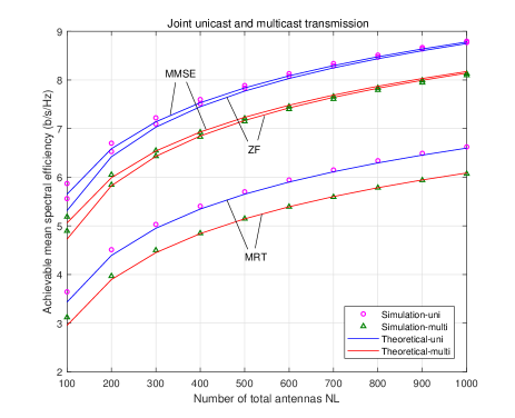
Figure 4: Spectral efficiency against the total number of antennas

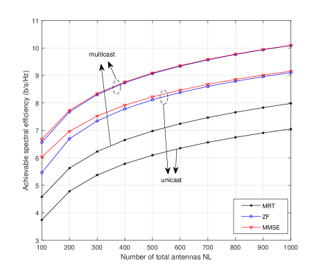
Figure 5: Comparison between multicast and unicast

Fig. 5 verifies the theoretical and simulation values of the achievable SE of unicast users and multigroup multicast users with MRT, ZF and MMSE precoding against the number of total antennas. It is illustrated that the simulation results agree well with the theoretical results we deduced, which verifies the accuracy of (20) and (21).

Since both RAUs and multigroup multicast users are dispersedly distributed in cell-free distributed massive MIMO scenarios. The distance from each multicast group to the RAUs is more even. Thus multigroup multicast users are less susceptible than unicast by the location of RAUs.

Fig. 5 illustrates the comparison of SE between unicast and multicast under the same parameters. We have twenty users in each mode and in multicast, the users are divided into four groups with five users in each group. To guarantee the fairness of the comparison, the user positions are set the same. The downlink transmitted power is set to 2 W for each multigroup and unicast user. However, as shown in Fig. 5, the achievable SE of multicast users is obviously higher than that of unicast users. It shows that in the same condition, the power utilization of multicast is higher than unicast and it can significantly increase the SE when the number of users in a multicast group is big.

Fig. 7 compares the SE of unicast and multicast against the coherence time $T$. The number of antennas per RAU is set to 50 and the coherence time $T$ is ranging from the number of pilots $\tau$ to 300. To avoid pilot contamination, it needs to be bigger than the number of unicast users or multicast groups. As shown in the figure, when $T$ is small, especially when $T$ is below 50, the achievable SE of multicast user is extremely higher than that of unicast user. This is because the demand of pilot cost is much lower in multicast. As a result, the advantage of multicast in reducing pilot cost can effectively enhance the SE of users especially when the coherence time $T$ is not relatively high.

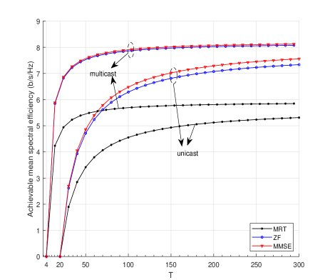
Figure 6: Spectral efficiency against the coherence time T

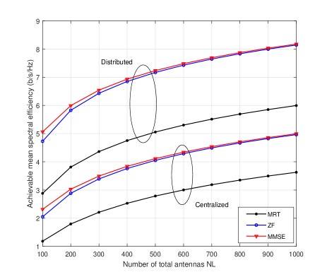
Figure 7: Comparison of multicast between distributed massive MIMO and centralized massive MIMO

Fig. 7 compares the SE of multicast in cell-free distributed massive MIMO and traditional centralized massive MIMO systems. The validity of multicast in centralized massive MIMO has already been indicated in [32], thus the SE of multicast under the two scenarios can be compared. The position of users, the number of total antennas and the other parameters are set exactly the same. It can be seen from the figure that the SE of multicast users in cell-free distributed massive MIMO is twice over that in centralized massive MIMO systems. Actually, it should be indicated that the performance of multicast in cell-free scenarios to some extent depends on the distribution of the RAUs and the multicast users. However, in most times it can achieve better performance due to the interactions between RAUs and the dispersed distribution of multicast users. As a result, combining cell-free scenarios with multicast can effectively improve the spectrum utilization of users.

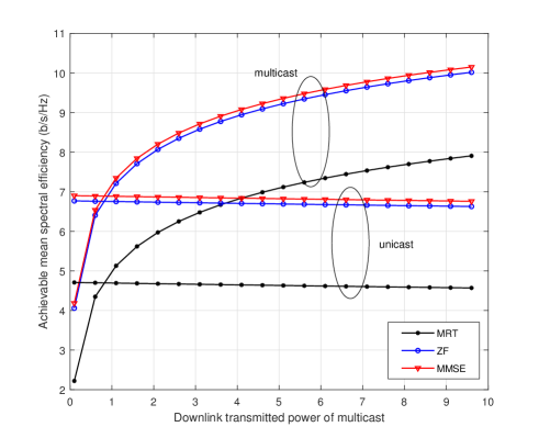
(a) noise power -10dbm.

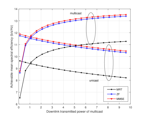
(b) noise power -15dbm.

Figure 8: Spectral efficiency against downlink transmitted power of multicast.

Fig. 8 illustrates the SE of unicast and multicast users against the downlink transmitted power of multicast. The number of antennas per RAU is set to 50 and it is assumed that the downlink transmitted power of multicast ranging from 0.1 W to 9.6 W and the power of unicast remains 1 W. Fig. 8(a) and Fig. 8(b) are the results under the noise power of -70 dBm and -120dbm respectively. The rest simulation parameters are set in accordance with Table I. It can be seen from the two figures that the SE of multicast users increases with the increasing downlink transmitted power of multicast groups, while the SE of unicast users are affected mildly and dropped slightly especially in Fig. 8(a). As a result, in joint unicast and multigroup multicast transmission, increasing the transmitted power of multicast can promote the SE of multicast and not cause a big trouble to unicast. This supports the feasibility of the joint unicast and multicast system proposed in this paper. Besides, under the condition of lower noise power, which means high signal-to-noise ratio (SNR), the downlink transmitted power of multicast has a greater impact on unicast. This is because both unicast and multicast are more sensitive to the interferences between them in high SNR cases. In these cases, the confliction between maximizing the SE of unicast and multicast are more obvious, which leads to the MOOP proposed in (31).

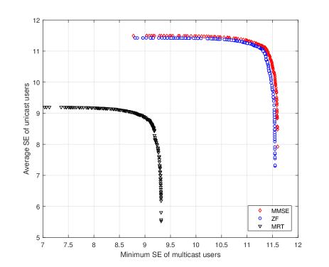
Figure 9: Trade-off between the minimum SE of multicast users and average SE of unicast users

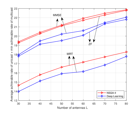
Figure 10: Comparison of the sum achieveable rate between NSGA-II and Deep Learning

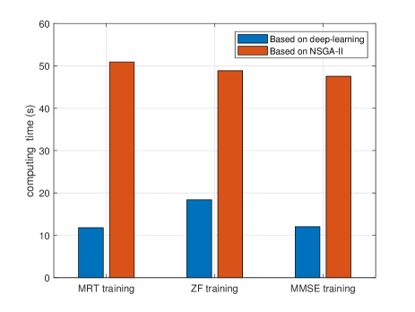
Figure 11: Comparison of elapsed time between NSGA-II and Deep Learning

Fig. 10 illustrates the trade-off between the minimum SE of multicast users and average SE of unicast users under different precoding schemes. The picture shows the Pareto boundary obtained by solving the MOOP (31) with NSGA-II. The number of antennas per RAU is set to 50. The upper limit of downlink transmitted power per RAU is given by 10W. The required minimum SE of both unicast and multicast users is set to 3 b/s/Hz. It can be seen that the minimum SE of multicast users increases with the decrease of the average SE of unicast users, which means that they can not achieve the highest value simultaneously and verifys the confliction between these two objectives in joint unicast and multigroup multicast transmission under cell-free distributed massive MIMO scenarios. As is marked in the picture, the approximately optimal value of the trade-off between multicast and unicast can be obtained by NSGA-II, which is also the optimal solution of the MOOP (31).

Fig. 10 illustrates the comparison of the maximum sum of average achievable rate of unicast users and minimum achievable rate of multicast users between NSGA-II and DL. We input the channel large-scale fading between 5 RAUs and 4 unicast users and 4 multicast users evenly divided into 2 multicast group to the DNN and the corresponding parameters in NSGA-II is set the same. To adapt the input environment of DL, the $2\times 2$ two-dimensional matrix and $5\times 2\times 2$ three-dimensional matrix need to be merged into one matrix and reshaped into a $1\times 40$ column vector. The total power for downlink transmission are 47 W. To set a higher standard, we select the best point of the sum rate in NSGA-II for comparison. It can be seen from the figure that the sum rate obtained by DL can achieve above 92$\%$ of the highest rate obtained by NSGA-II. Fig. 11 shows the elapsed time of DL and NSGA-II with $L=60$. In DL, it only takes about 14 seconds to train, however, with NSGA-II, it takes about 50 seconds, which is above 3.5 times of the elapsed time with DL. The effect of NSGA-II algorithm optimization is quite good, but the calculation time is long and the complexity is high. In DL, the optimization method is to train the loss function to the lowest, so the result will be affected by some neural network parameters and the performance will not achieve the best, but the optimization time of DL is quite short and it is considerable for DL to be close to NSGA-II.

VIII Conclusion

In this paper, we studied the joint unicast and multigroup multicast transmission in cell-free distributed massive MIMO systems. With the estimated CSI obtained by co-pilot assignment strategy, we deduced the closed-form expression of downlink SE of unicast users and multicast users with MRT, ZF and MMSE precoding schemes. With these expressions, we proposed a MOOP between the MMF of multicast and the maximum of the average SE of unicast under several constraints. Based on the MOOP, we further converted it into a DL problem to reduce computational complexity. We verified the derived closed-form expressions by Monte Carlo simulation and compared the SE of unicast and multicast under the same parameters to show that multicast can achieve higher SE and occupy less coherence time slots. Besides, it was verified that the combination of distributed massive MIMO systems and multicast transmission can effectively achieve higher SE. The effects of downlink transmitted power and noise power on SE were analyzed and the two objectives in the proposed MOOP was proved conflicting. The trade-off region between these two conflicting problems obtained with NSGA-II under various constraints offered numerous flexibilities for system optimization. Furthermore, the comparison between NSGA-II and DL showed that solving the MOOP by DL can also achieve relatively good results with quite short elapsed time and low complexity.

Appendix A Proof of Theorem 1

We first calculate the needed signal for unicast users (MMSE as an example). By substituting the MMSE precoding vector into the item $\mathbb{E}\left[\mathbf{c}_{k}^{\mathrm{H}}\mathbf{v}_{{k}}^{\mathrm{pre}}\right]$ , we have

$$\mathbb{E}\left[\mathbf{c}_{k}^{\mathrm{H}}\mathbf{v}_{{k}}^{\mathrm{MMSE}}\right] =\mathbb{E}\left[\mathbf{c}_{k}^{\mathrm{H}}\sqrt{\frac{p_{\text{dl},k}{{(A{{\theta}_{k}}+\sigma_{\mathrm{dl}}^{2})}^{2}}}{A{{\theta}_{k}}}}{{\chi}_{k}}\right]$$

$$=\sqrt{\frac{p_{\mathrm{dl},k}{{(A{{\theta}_{k}}+\sigma_{\mathrm{dl}}^{2})}^{2}}}{A{{\theta}_{k}}}}{{(A{{\theta}_{k}}+\sigma_{\mathrm{dl}}^{2})}^{-1}}NL{{\theta}_{k}}$$

$$=\sqrt{\frac{{{\left(NL\right)}^{2}}p_{\mathrm{dl},k}{{\theta}_{k}}}{A}},$$ (A1)

where ${{\chi}_{k}}=\left[\mathbf{\hat{Q}}{{(\overset{{}}{\mathop{{{{\mathbf{\hat{Q}}}}^{\mathrm{H}}}\mathbf{\hat{Q}+}\sigma_{\mathrm{dl}}^{2}}}\,\otimes{\mathbf{I}_{NL}})}^{-1}}\right]_{k}$.

Then, for the denominator part $\mathbb{E}\left[{{\left|\mathbf{c}_{k}^{\mathrm{H}}\mathbf{v}_{u}^{\mathrm{MMSE}}\right|}^{2}}\right]$, when $u=k$, due to the independence of $\mathbf{c}_{k}$ and ${\mathbf{n}}_{k}$, we have $\mathbb{E}\left[\mathbf{c}_{k}{{\mathbf{n}}_{k}}\right]=0$, and we can obtain

$$\mathbb{E}\left[{{\left|\mathbf{c}_{k}^{\mathrm{H}}\mathbf{v}_{k}^{\mathrm{MMSE}}\right|}^{2}}\right]$$

$$= \,\frac{p_{\mathrm{dl},k}{{(A{{\theta}_{k}}+\sigma_{\mathrm{dl}}^{2})}^{2}}}{A{{\theta}_{k}}}\mathbb{E}\left[\left(\mathbf{c}_{k}^{\mathrm{H}}{{\chi}_{k}}\right){{\left({{\chi}_{k}^{\mathrm{H}}}\mathbf{c}_{k}\right)}}\right]$$

$$= \,p_{\mathrm{dl},k}{{\left(A{{\theta}_{k}}\right)}^{-1}}\mathbb{E}\left[\mathbf{c}_{k}^{\mathrm{H}}\mathbf{\hat{c}}_{k}\mathbf{\hat{c}}_{k}^{\mathrm{H}}\mathbf{c}_{k}\right]$$

$$\overset{(a)}{=} \,\frac{p_{\mathrm{dl},k}\mathbb{E}\left[\mathbf{c}_{k}^{\mathrm{H}}(\sqrt{\tau p_{\mathrm{ul},k}}{{\mathbf{c}}_{k}}+{{\mathbf{n}}_{k}}){{(\sqrt{\tau p_{\mathrm{ul},k}}{{\mathbf{c}}_{k}}+{{\mathbf{n}}_{k}})}^{\mathrm{H}}}\mathbf{c}_{k}\right]}{A\left(\tau p_{\mathrm{ul},k}\sum\limits_{n=1}^{N}{{{\beta}_{n,k}}}+\sigma_{\mathrm{ul}}^{2}\right)}$$

$$\overset{(b)}{=} \,\frac{p_{\mathrm{dl},k}\left(\tau p_{\mathrm{ul},k}{{\left(NL\sum\limits_{n=1}^{N}{{{\beta}_{n,k}}}\right)}^{2}}\right)}{A\left(\tau p_{\mathrm{ul},k}\sum\limits_{n=1}^{N}{{{\beta}_{n,k}}}+\sigma_{\mathrm{ul}}^{2}\right)}+\frac{1}{NL}p_{\mathrm{dl},k}\sum\limits_{n=1}^{N}{{{\beta}_{n,k}}}$$

$$= \,\frac{{{\left(NL\right)}^{2}}p_{\mathrm{dl},k}{{\theta}_{k}}}{A}+\frac{1}{NL}p_{\mathrm{dl},k}\sum\limits_{n=1}^{N}{{{\beta}_{n,k}}},$$ (A2)

where (a) is obtained by plugging $\theta_{k}$ into (II-C) and (b) is got by means of uncorrelated vectors and the large-scale random matrix conclusions[45].

Lemma ([45]): If $\mathbf{A}\in{{C}^{M\times M}}$ has the uniformly bounded spectral norm (relative to $M$), vector x and y follows $\mathcal{C}\mathcal{N}\left(0,\frac{1}{M}{{\mathbf{I}}_{M}}\right)$, and x, y is independent of each other and matrix A, it has

$${{\mathbf{x}}^{\mathrm{H}}}\mathbf{Ay}\xrightarrow[M\to\infty]{a.s.}0$$

$${{\mathbf{x}}^{\mathrm{H}}}\mathbf{Ax}-\frac{1}{M}\mathrm{Tr}\left(\mathbf{A}\right)\xrightarrow[M\to\infty]{a.s.}0$$

When $u\neq k$,

$$\mathbb{E}\left[{{\left|\mathbf{c}_{k}^{\mathrm{H}}\mathbf{v}_{u}^{\mathrm{MMSE}}\right|}^{2}}\right] =\frac{1}{NL}p_{\mathrm{dl},u}\sum\limits_{n=1}^{N}{{{\beta}_{n,k}}}.$$ (A3)

For the denominator part $\mathbb{E}\left[{{\left|\mathbf{c}_{k}^{\mathrm{H}}\mathbf{w}_{r}^{\mathrm{MMSE}}\right|}^{2}}\right]$, based on large-scale random matrix theory, we have

$$\mathbb{E}\left[{{\left|\mathbf{c}_{k}^{\mathrm{H}}\mathbf{w}_{r}^{\mathrm{MMSE}}\right|}^{2}}\right] =\frac{1}{NL}q_{\mathrm{dl},r}\sum\limits_{n=1}^{N}{{{\beta}_{n,k}}}.$$ (A4)

The conclusion can be proved by substituting the values of the above fractions into (18).

For multicast, we can calculate the needed signal for user (Molecularpart) similarly, by substituting the preocoding vector, we have

$$\mathbb{E}\left[\mathbf{t}_{m,k}^{\mathrm{H}}\mathbf{w}_{m}^{\mathrm{MMSE}}\right]$$

$$= \,\sqrt{q_{\mathrm{dl},m}\frac{{{(A{{\upsilon}_{m}}+\sigma_{\mathrm{dl}}^{2})}^{2}}}{A{{\upsilon}_{m}}}}\mathbb{E}\left[\mathbf{t}_{m,k}^{\mathrm{H}}{{\chi}_{m}}\right]$$

$$\overset{\text{(a)}}{=} \,\sqrt{q_{\mathrm{dl},m}\frac{{{(A{{\upsilon}_{m}}+\sigma_{\mathrm{dl}}^{2})}^{2}}}{A{{\upsilon}_{m}}}}\frac{NL\sum\limits_{n=1}^{N}{{\kappa}_{n,m}}\sqrt{\tau q_{\mathrm{ul},m,k}}{\eta_{n,m,k}}}{{{(A{{\upsilon}_{m}}+\sigma_{\mathrm{dl}}^{2})}}}$$

$${=} \,\sqrt{\frac{{{\left(NL\right)}^{2}}q_{\mathrm{dl},m}{{\zeta}_{m,k}}}{A}},$$ (A5)

where ${{\chi}_{m}}=\left[\mathbf{\hat{Q}}{{\left({\mathop{{{{\mathbf{\hat{Q}}}}^{\mathrm{H}}}\mathbf{\hat{Q}+}\sigma_{\mathrm{dl}}^{2}}}\,\otimes{\mathbf{I}_{NL}}\right)}^{-1}}\right]_{U+m},{{\kappa}_{n,m}}=$ ${\sum\nolimits_{j=1}^{{{K}_{m}}}{\tau q_{\mathrm{ul},m,j}\eta_{n,m,j}}}/\left({\sum\nolimits_{j=1}^{{{K}_{m}}}{\tau q_{\mathrm{ul},m,j}\eta_{n,m,j}}+\sigma_{\mathrm{ul}}^{2}}\right),{{\zeta}_{m,k}}=\sum_{n=1}^{N}{\frac{\tau q_{\mathrm{ul},m,k}\eta_{n,m,k}^{2}}{\sum\nolimits_{j=1}^{{{K}_{m}}}{\tau q_{\mathrm{ul},m,j}{{\eta}_{n,m,j}}}+\sigma_{\mathrm{ul}}^{2}}}$, (a) is obtained by large-scale random matrix conclusions [45].

For the denominator part $\mathbb{E}\left[{{\left|\mathbf{t}_{m,k}^{\mathrm{H}}{{\mathbf{w}}_{r}^{\mathrm{MMSE}}}\right|}^{2}}\right]$, when $r=m$, we have

$$\mathbb{E}\left[{{\left|\mathbf{t}_{m,k}^{\mathrm{H}}\mathbf{w}_{m}^{\mathrm{MMSE}}\right|}^{2}}\right]$$

$$= q_{\mathrm{dl},m}\frac{{{(A{{\upsilon}_{m}}+\sigma_{\mathrm{dl}}^{2})}^{2}}}{A{{\upsilon}_{m}}}\mathbb{E}\left[\left(\mathbf{t}_{m,k}^{\mathrm{H}}{{\chi}_{m}}\right){{\chi}_{m}}^{\mathrm{H}}\mathbf{t}_{m,k}\right].$$ (A6)

Then, for the term $\mathbb{E}\left[\left(\mathbf{t}_{m,k}^{\mathrm{H}}{{\chi}_{m}}\right){{\chi}_{m}}^{\mathrm{H}}\mathbf{t}_{m,k}\right]$, due to the large-scale random matrix theory [45], we have

$$\mathbb{E}\left[\left(\mathbf{t}_{m,k}^{\mathrm{H}}{{\chi}_{m}}\right){{\chi}_{m}}^{\mathrm{H}}\mathbf{t}_{m,k}\right]$$

$$= \,\frac{\mathbb{E}\Big{[}\mathbf{t}_{m,k}^{\mathrm{H}}\big{[}\mathbf{\hat{Q}}\big{]}_{U+m}\Big{(}\big{[}\mathbf{\hat{Q}}\big{]}_{U+m}\Big{)}^{\mathrm{H}}\mathbf{t}_{m,k}\Big{]}}{(A{{\upsilon}_{m}}+\sigma_{\mathrm{dl}}^{2})^{2}}$$

$$= \,\frac{\sum\limits_{n=1}^{N}{{\kappa}_{n,m}}tr\left(\tau q_{\mathrm{ul},m,k}\sum\nolimits_{j=1}^{{{K}_{m}}}\mathcal{I}_{gj,m,k}+\mathcal{I}_{gn,m,k}\right)}{(A{{\upsilon}_{m}}+\sigma_{\mathrm{dl}}^{2})^{2}}.$$ (A7)

Based on the above analysis and combining the result into (A), we obtain

$$\mathbb{E}\left[{{\left|\mathbf{t}_{m,k}^{\mathrm{H}}\mathbf{w}_{m}^{\mathrm{MMSE}}\right|}^{2}}\right]$$

$$= \,\frac{q_{\mathrm{dl},m}\Big{(}\tau q_{\mathrm{ul},m,k}{{\big{(}NL\sum_{n=1}^{N}{\eta_{n,m,k}}\big{)}}^{2}}\Big{)}}{A\left(\sum_{n=1}^{N}{\left(\sum_{j=1}^{{{K}_{m}}}{\tau q_{\mathrm{ul},m,j}\eta_{n,m,j}}+\sigma_{\mathrm{ul}}^{2}\right)}\right)}$$

$$+\frac{1}{NL}q_{\mathrm{dl},m}\sum_{n=1}^{N}{\eta_{n,m,k}}$$

$$= \,\frac{{{\left(NL\right)}^{2}}q_{\mathrm{dl},m}{\zeta_{m,k}}}{A}+\frac{1}{NL}q_{\mathrm{dl},m}\sum\limits_{n=1}^{N}{\eta_{n,m,k}}.$$ (A8)

When $r\neq m$,

$$\mathbb{E}\left[{{\left|\mathbf{t}_{m,k}^{\mathrm{H}}\mathbf{w}_{r}^{\mathrm{MMSE}}\right|}^{2}}\right] =\frac{1}{NL}q_{\mathrm{dl}}\sum\limits_{n=1}^{N}{\eta_{n,m,k}}.$$ (A9)

Then, to the other denominator part

$$\mathbb{E}\left[{{\left|\mathbf{t}_{m,k}^{\mathrm{H}}\mathbf{v}_{u}^{\mathrm{MMSE}}\right|}^{2}}\right] =\frac{1}{NL}p_{\mathrm{dl},u}\sum\limits_{n=1}^{N}{{{\eta}_{n,m,k}}}.$$ (A10)

The conclusion can be proved by combining the results of the above fractions into (19). The closed-form expression of ZF can be derived similarly and the derivation of the needed signals with MRT have some difference and is given below

$$\mathbb{E}\left[\mathbf{c}_{k}^{\mathrm{H}}\mathbf{v}_{k}^{\mathrm{MRT}}\right]$$

$$= \sqrt{\frac{p_{\mathrm{dl},k}}{L{\theta}_{k}}}\mathbb{E}\left[\mathbf{c}_{k}^{\mathrm{H}}{{{\mathbf{\hat{c}}}}_{k}}\right]$$

$$= \,\sqrt{\frac{p_{\mathrm{dl},k}}{L{{\theta}_{k}}}}\sum\limits_{n=1}^{N}{\frac{\sqrt{\tau p_{\mathrm{ul},k}}{{\beta}_{n,k}}}{\sigma_{\mathrm{ul}}^{2}{{\mathbf{I}}_{NL}}\text{+}\tau p_{\mathrm{ul},k}{{\beta}_{n,k}}}}\left(\begin{aligned} &\sqrt{\tau p_{\mathrm{ul},k}}\mathbb{E}\left[\mathbf{c}_{k}^{\mathrm{H}}{{\mathbf{c}}_{k}}\right]\\ &+\mathbb{E}\left[\mathbf{c}_{k}^{\mathrm{H}}{{\mathbf{n}}_{k}}\right]\end{aligned}\right)$$

$${\overset{\text{(a)}}{=}} \,\sqrt{\frac{p_{\mathrm{dl},k}}{L{{\theta}_{k}}}}\sum\limits_{n=1}^{N}{\frac{L\tau p_{\mathrm{ul},k}{{\beta}_{n,k}}^{2}}{\sigma_{\mathrm{ul}}^{2}{{\mathbf{I}}_{NL}}\text{+}\tau p_{\mathrm{ul},k}{{\beta}_{n,k}}}}$$

$$= \,\sqrt{Lp_{\mathrm{dl},k}{{\theta}_{k}}},$$ (A11)

where (a) is got by the uncorrelated vectors between channels and noises and the large-scale random matrix conclusions.

$$\mathbb{E}\left[\mathbf{t}_{m,k}^{\mathrm{H}}\mathbf{w}_{m}^{\mathrm{MRT}}\right]$$

$$= \,\sqrt{\frac{q_{\text{dl},m}}{L{{\upsilon}_{m}}}}\mathbb{E}\left[\mathbf{t}_{m,k}^{\mathrm{H}}{{{\mathbf{\hat{t}}}}_{m}}\right]$$

$$= \,\sqrt{\frac{q_{\mathrm{dl},m}}{L{{\upsilon}_{m}}}}\sum\limits_{n=1}^{N}{{\kappa}_{n,m}}\sqrt{\tau q_{\mathrm{ul},m,k}}\mathbb{E}\left[\mathbf{t}_{m,k}^{\mathrm{H}}\mathbf{t}_{m,k}\right]$$

$${\overset{\text{(b)}}{=}} \,\sqrt{\frac{q_{\mathrm{dl},m}\left(L\sum_{n=1}^{N}{{\kappa}_{n,m}}\sqrt{\tau q_{\mathrm{ul},m,k}}L\sum_{n=1}^{N}{\eta_{n,m,k}}\right)^{2}}{\sum_{n=1}^{N}{\frac{{{(\sum_{j=1}^{{{K}_{m}}}{\tau q_{\mathrm{ul},m,j}{{\eta}_{n,m,j}}})}^{2}}}{\sum_{j=1}^{{{K}_{m}}}{\tau q_{\mathrm{ul},m,j}{{\eta}_{n,m,j}}}+\sigma_{\mathrm{ul}}^{2}}}}}$$

$$= \,\sqrt{\sum\limits_{n=1}^{N}{\frac{Lq_{\mathrm{dl},m}\tau q_{\mathrm{ul},m,k}\eta_{n,m,k}^{2}}{\sum\nolimits_{j=1}^{{{K}_{m}}}{\tau q_{\mathrm{ul},m,j}\eta_{n,m,j}}+\sigma_{\mathrm{ul}}^{2}}}}$$

$$= \,\sqrt{Lq_{\mathrm{dl},m}{{\zeta}_{m,k}}},$$ (A12)

where (b) is obtained by large-scale random matrix conclusions.

Jiamin Li received the B.S. and M.S. degrees in communication and information systems from Hohai University, Nanjing, China, in 2006 and 2009, respectively, and the Ph.D. degree in information and communication engineering from Southeast University, Nanjing, China, in 2014. He joined the National Mobile Communications Research Laboratory, Southeast University, in 2014, where he has been an Associate Professor since 2019. His research interests include massive MIMO, distributed antenna systems, and multi-objective optimization.

Qijun Pan was born in Shanghai province, China, in 1998. She received the B.S. degree in the school of communication and information engineering from Shanghai University, Shanghai, China, in 2020. She is currently pursuing the M.S. degree in electronic and communication engineering at the National Mobile Communications Research Laboratory, Southeast University. Her research interests include massive MIMO, distributed antenna systems and ultra reliable low latency communication.

Zhenggang Wu was born in Yangzhou, Jiangsu province, China. He received the B.S. degree in communication engineering from Hohai University, Nanjing, China, in 2020. He is currently working toward the M.S. degree in electronic and communication engineering at the National Mobile Communications Research Laboratory, Southeast University. His research interests mainly include massive MIMO, ultrareliable low latency communication, 3D coverage and massive access.

Pengcheng Zhu received the B.S and M.S. degrees in electrical engineering from Shandong University, Jinan, China, in 2001 and 2004, respectively, and the Ph.D. degree in communication and information science from the Southeast University, Nanjing, China, in 2009. He has been a lecturer with the national mobile communications research laboratory, Southeast University, China, since 2009. His research interests lie in the areas of communication and signal processing, including limited feedback techniques, and distributed antenna systems.

Dongming Wang received the B.S. degree from Chongqing University of Posts and Telecommunications, Chongqing, China, the M.S. degree from Nanjing University of Posts and Telecommunications, Nanjing, China, and the Ph.D. degree from the Southeast University, Nanjing, China, in 1999, 2002, and 2006, respectively. He joined the National Mobile Communications Research Laboratory, Southeast University, in 2006, where he has been an Associate Professor since 2010. His research interests include turbo detection, channel estimation, distributed antenna systems, and large-scale MIMO systems.

Xiaohu You (Fellow, IEEE) received the B.S., M.S. and Ph.D. degrees in electrical engineering from Nanjing Institute of Technology, Nanjing, China, in 1982, 1985, and 1989, respectively. From 1987 to 1989, he was with Nanjing Institute of Technology as a Lecturer. From 1990 to the present time, he has been with Southeast University, first as an Associate Professor and later as a Professor. His research interests include mobile communications, adaptive signal processing, and artificial neural networks with applications to communications and biomedical engineering. He is the Chief of the Technical Group of China 3G/B3G Mobile Communication R & D Project. He received the excellent paper prize from the China Institute of Communications in 1987 and the Elite Outstanding Young Teacher Awards from Southeast University in 1990, 1991, and 1993. He was also a recipient of the 1989 Young Teacher Award of Fok Ying Tung Education Foundation, State Education Commission of China.

References

- [1] E. Nayebi, A. Ashikhmin, T. L. Marzetta, and H. Yang, “Cell-free massive MIMO systems,” in 49th Asilomar Conference on Signals, Systems and Computers, Nov. 2015, pp. 695–699.
- [2] S. Buzzi, C. D’Andrea, A. Zappone, and C. D’Elia, “User-centric 5G cellular networks: Resource allocation and comparison with the cell-free massive MIMO approach,” IEEE Trans. Wireless Commun., vol. 19, no. 2, pp. 1250–1264, Nov. 2019.
- [3] H. Q. Ngo, A. Ashikhmin, H. Yang, E. G. Larsson, and T. L. Marzetta, “Cell-free massive MIMO uniformly great service for everyone,” in IEEE 16th international workshop on signal processing advances in wireless communications (SPAWC), Jun. 2015, pp. 201–205.
- [4] J. Li, D. Wang, P. Zhu, J. Wang, and X. You, “Downlink spectral efficiency of distributed massive MIMO systems with linear beamforming under pilot contamination,” IEEE Transactions on Vehicular Technology, vol. 67, no. 2, pp. 1130–1145, Jul. 2017.
- [5] P. Parida, H. S. Dhillon, and A. F. Molisch, “Downlink performance analysis of cell-free massive MIMO with finite fronthaul capacity,” in IEEE 88th Vehicular Technology Conference (VTC-Fall), Aug. 2018, pp. 1–6.
- [6] F. Riera-Palou and G. Femenias, “Decentralization issues in cell-free massive MIMO networks with Zero-Forcing precoding,” in 2019 57th Annual Allerton Conference on Communication, Control, and Computing (Allerton), Sept. 2019, pp. 521–527.
- [7] E. Yaacoub, M. Husseini, and H. Ghaziri, “An overview of research topics and challenges for 5G massive MIMO antennas,” in IEEE Middle East Conference on Antennas and Propagation (MECAP), Dec. 2016, pp. 1–4.
- [8] E. G. Larsson and H. V. Poor, “Joint beamforming and broadcasting in massive MIMO,” IEEE Transactions on Wireless Communications, vol. 15, no. 4, pp. 3058–3070, Jan. 2016.
- [9] J. Zhang, S. Chen, Y. Lin, J. Zheng, B. Ai, and L. Hanzo, “Cell-free massive mimo: A new next-generation paradigm,” IEEE Access, vol. 7, pp. 99 878–99 888, 2019.
- [10] H. A. Ammar, R. Adve, S. Shahbazpanahi, G. Boudreau, and K. V. Srinivas, “User-centric cell-free massive mimo networks: A survey of opportunities, challenges and solutions,” IEEE Communications Surveys & Tutorials, 2021.
- [11] D. Wang, C. Zhang, Z. Ji, Y. Du, J. Zhao, M. Jiang, and X. You, “Live demonstration: A cloud-based cell-free distributed massive mimo system,” in 2021 IEEE International Symposium on Circuits and Systems (ISCAS). IEEE, 2021, pp. 1–1.
- [12] A. Papazafeiropoulos, P. Kourtessis, M. Di Renzo, S. Chatzinotas, and J. M. Senior, “Performance analysis of cell-free massive mimo systems: A stochastic geometry approach,” IEEE Transactions on Vehicular Technology, vol. 69, no. 4, pp. 3523–3537, 2020.
- [13] P. Liu, K. Luo, D. Chen, and T. Jiang, “Spectral efficiency analysis of cell-free massive mimo systems with zero-forcing detector,” IEEE Transactions on Wireless Communications, vol. 19, no. 2, pp. 795–807, 2019.
- [14] G. Femenias, F. Riera-Palou, A. Álvarez-Polegre, and A. García-Armada, “Short-term power constrained cell-free massive-mimo over spatially correlated ricean fading,” IEEE Transactions on Vehicular Technology, vol. 69, no. 12, pp. 15 200–15 215, 2020.
- [15] Y. Zhang and L. Dai, “A closed-form approximation for uplink average ergodic sum capacity of large-scale multi-user distributed antenna systems,” IEEE Transactions on Vehicular Technology, vol. 68, no. 2, pp. 1745–1756, 2019.
- [16] Y. Hu, F. Zhang, C. Li, Y. Wang, and R. Zhao, “Energy efficiency resource allocation in downlink cell-free massive mimo system,” in 2017 International Symposium on Intelligent Signal Processing and Communication Systems (ISPACS). IEEE, 2017, pp. 878–882.
- [17] S. Mosleh, H. Almosa, E. Perrins, and L. Liu, “Downlink resource allocation in cell-free massive mimo systems,” in 2019 International Conference on Computing, Networking and Communications (ICNC). IEEE, 2019, pp. 883–887.
- [18] B. Amin, B. Abdelhamid, and S. El-Ramly, “Quantized power allocation algorithms in cell-free massive mimo systems,” in 2018 International Japan-Africa Conference on Electronics, Communications and Computations (JAC-ECC). IEEE, 2018, pp. 35–38.
- [19] F. Riera-Palou and G. Femenias, “Trade-offs in cell-free massive mimo networks: Precoding, power allocation and scheduling,” in 2019 14th International Conference on Advanced Technologies, Systems and Services in Telecommunications (TELSIKS). IEEE, 2019, pp. 158–165.
- [20] A. Izadi, S. M. Razavizadeh, and O. Saatlou, “Power allocation for downlink training in cell-free massive mimo networks,” in 2020 10th International Symposium onTelecommunications (IST). IEEE, 2020, pp. 111–115.
- [21] S. Chakraborty, Ö. T. Demir, E. Björnson, and P. Giselsson, “Efficient downlink power allocation algorithms for cell-free massive mimo systems,” IEEE Open Journal of the Communications Society, vol. 2, pp. 168–186, 2020.
- [22] Z. Chen, E. Björnson, and E. G. Larsson, “Dynamic resource allocation in co-located and cell-free massive mimo,” IEEE Transactions on Green Communications and Networking, vol. 4, no. 1, pp. 209–220, 2019.
- [23] V. M. Palhares, A. R. Flores, and R. C. de Lamare, “Robust mmse precoding and power allocation for cell-free massive mimo systems,” IEEE Transactions on Vehicular Technology, vol. 70, no. 5, pp. 5115–5120, 2021.
- [24] J. Ding, D. Qu, P. Liu, and J. Choi, “Machine learning enabled preamble collision resolution in distributed massive mimo,” IEEE Transactions on Communications, vol. 69, no. 4, pp. 2317–2330, 2021.
- [25] N. D. Sidiropoulos, T. N. Davidson, and Z.-Q. Luo, “Transmit beamforming for physical-layer multicasting,” IEEE transactions on signal processing, vol. 54, no. 6, pp. 2239–2251, Jun. 2006.
- [26] E. Karipidis, N. D. Sidiropoulos, and Z.-Q. Luo, “Quality of service and max-min fair transmit beamforming to multiple cochannel multicast groups,” IEEE Transactions on Signal Processing, vol. 56, no. 3, pp. 1268–1279, Feb. 2008.
- [27] H. Yang, T. L. Marzetta, and A. Ashikhmin, “Multicast performance of large-scale antenna systems,” in IEEE 14th Workshop on Signal Processing Advances in Wireless Communications (SPAWC), Sept. 2013, pp. 604–608.
- [28] M. Sadeghi, L. Sanguinetti, R. Couillet, and C. Yuen, “Reducing the computational complexity of multicasting in large-scale antenna systems,” IEEE Transactions on Wireless Communications, vol. 16, no. 5, pp. 2963–2975, Mar. 2017.
- [29] D. Christopoulos, S. Chatzinotas, and B. Ottersten, “Multicast multigroup beamforming for per-antenna power constrained large-scale arrays,” in IEEE 16th International Workshop on Signal Processing Advances in Wireless Communications (SPAWC), Aug. 2015, pp. 271–275.
- [30] M. Dong and Q. Wang, “Multi-group multicast beamforming: Optimal structure and efficient algorithms,” IEEE Transactions on Signal Processing, vol. 68, pp. 3738–3753, May 2020.
- [31] A. Bandi, R. B. S. Mysore, S. Chatzinotas, and B. Ottersten, “Joint user scheduling, and precoding for multicast spectral efficiency in multigroup multicast systems,” in International Conference on Signal Processing and Communications (SPCOM), Aug. 2020, pp. 1–5.
- [32] M. Sadeghi, E. Björnson, E. G. Larsson, C. Yuen, and T. Marzetta, “Joint unicast and multi-group multicast transmission in massive MIMO systems,” IEEE Transactions on Wireless Communications, vol. 17, no. 10, pp. 6375–6388, 2018.
- [33] T. X. Doan, H. Q. Ngo, T. Q. Duong, and K. Tourki, “On the performance of multigroup multicast cell-free massive MIMO,” IEEE Commun. Lett., vol. 21, no. 12, pp. 2642–2645, Aug. 2017.
- [34] Y. Zhang, H. Cao, and L. Yang, “Max-min power optimization in multigroup multicast cell-free massive MIMO,” in IEEE Wireless Communications and Networking Conference (WCNC), Apr. 2019, pp. 1–6.
- [35] F. Tan, P. Wu, Y.-C. Wu, and M. Xia, “Energy-efficient non-orthogonal multicast and unicast transmission of cell-free massive MIMO systems with SWIPT,” IEEE J. Sel. Areas Commun., Sep. 2020.
- [36] X. Zhang, D. Guo, K. An, Z. Ding, and B. Zhang, “Secrecy analysis and active pilot spoofing attack detection for multigroup multicasting cell-free massive MIMO systems,” IEEE Access, vol. 7, pp. 57 332–57 340, Apr. 2019.
- [37] E. Björnson, M. Matthaiou, and M. Debbah, “Massive MIMO with non-ideal arbitrary arrays: Hardware scaling laws and circuit-aware design,” IEEE Transactions on Wireless Communications, vol. 14, no. 8, pp. 4353–4368, Apr. 2015.
- [38] S. K. Mohammed and E. G. Larsson, “Single-user beamforming in large-scale MISO systems with per-antenna constant-envelope constraints: The doughnut channel,” IEEE Transactions on Wireless Communications, vol. 11, no. 11, pp. 3992–4005, Sept. 2012.
- [39] X. Yu, J.-C. Shen, J. Zhang, and K. B. Letaief, “Alternating minimization algorithms for hybrid precoding in millimeter wave MIMO systems,” IEEE Journal of Selected Topics in Signal Processing, vol. 10, no. 3, pp. 485–500, Feb. 2016.
- [40] H. Q. Ngo, E. G. Larsson, and T. L. Marzetta, “Energy and spectral efficiency of very large multiuser MIMO systems,” IEEE Transactions on Communications, vol. 61, no. 4, pp. 1436–1449, Feb. 2013.
- [41] K. Deb, A. Pratap, S. Agarwal, and T. Meyarivan, “A fast and elitist multiobjective genetic algorithm: NSGA-II,” IEEE transactions on evolutionary computation, vol. 6, no. 2, pp. 182–197, Aug. 2002.
- [42] W. S. A. Qatab, M. Y. Alias, and I. Ku, “Optimization of multi-objective resource allocation problem in cognitive radio LTE/LTE-A femtocell networks using NSGA II,” in Proc. IEEE Int. Symposium on Telecommun. Technol. (ISTT), Nov 2018, pp. 1–6.
- [43] Y. LeCun, Y. Bengio, and G. Hinton, “Deep learning,” nature, vol. 521, no. 7553, pp. 436–444, 2015.
- [44] K. Kim, J. Lee, and J. Choi, “Deep learning based pilot allocation scheme (DL-PAS) for 5G massive MIMO system,” IEEE Communications Letters, vol. 22, no. 4, pp. 828–831, Feb. 2018.
- [45] D. Wang, M. Wang, P. Zhu, J. Li, J. Wang, and X. You, “Performance of network-assisted full-duplex for cell-free massive MIMO,” IEEE Transactions on Communications, vol. 68, no. 3, pp. 1464–1478, Dec. 2019.