Smeared Mass Source Wormholes in Modified $f(R)$ Gravity with the Lorentzian Density Distribution Function

Abstract

Wormholes are speculative structures linking disparate space-time points. Their geometry can be obtained by solving Einstein equations with tolerating the violation of null energy conditions. Recently, many researchers have studied different wormholes according to different criteria, and they achieved remarkable results. In this paper, we investigate a series of exact solutions of the static wormhole with smeared mass source geometry in modified $f(R)$ gravity theories. In fact, we consider the Lorentzian density distribution which is coming from a particle-like source. To be more specific, the modified gravity models we consider here are some power laws. We compute resulting solutions according to the wormhole field equations. We also specify parameters such as the radial pressure and transverse pressure as well as various energy conditions such as null energy conditions, weak energy conditions and strong energy conditions. Finally, by plotting some figures, in addition to identifying the wormhole throat, we describe the results of either the violation or the satisfaction of the energy conditions completely.

1 Introduction

The concept of wormhole, in general, was first introduced by Flamm in 1916 [1]. However, a few years later, Einstein and Rosen explored a similar structure with concept of wormhole in 1935, and they introduced a similar geometric structure which is called the Einstein-Rosen Bridge [2]. In fact, recently, wormholes have been evaluated by many researchers according to different criteria. In following, we will introduce a number of these studies. Actually, wormhole is a speculative structure linking disparate space-time points and is based on a particular solution of the Einstein field equations. A wormhole can be visualized as a tunnel with two ends at separate points in space-time, i.e., different locations, various points in time, or both[3]). Geometry of static symmetrical spherical wormholes consists of a two-state tunnel is usually considered in the literature which is called different names such as throat, tube or handle. In general, it is possible for a two-way journey if both distinct points belong to the same space-time. In the last few years, wormholes have been studied from different points of view [4, 5].

Different types of wormholes have been evaluated in different conditions in the literature, including cylindrical symmetry, non-static symmetries, conditions supported by cosmological constants, thin shells and static wormholes with electric charge, as well as various other types that have been explored by researchers over the past few years. However, despite all these studies, the wormhole is still a hypothetical object and no mechanism has been introduced to observe it, see Refs. [6, 7, 8, 9, 10, 11, 12, 13, 14, 15, 16, 17, 18, 19, 20] for further reading. Perhaps one of the most interesting and exciting types of wormholes is the traversable wormholes [21, 22]. In addition to the above issues, wormholes have also been studied from a cosmological point of view [23]. In fact, all of these studies with different criteria to find out the truth of what is hidden in the universe and researchers beings seek to discover its facts. Despite all these issues raised, wormholes exhibit a number of esoteric properties behaviors, such as violation of Hawking chronology protection conjecture, and in fact pursue cases that are associated with speed beyond light, or in other words, violation of causality [24, 25, 26, 27, 28, 29, 30, 31, 32, 33, 34, 35, 36]. In fact, the issue we are talking about is that the energy of matter, which is somehow supported by an exotic geometry, leads to a violation of the standard energy conditions. To avoid such problems, a series of modified $f(R)$ gravity theories are used in the studies related to wormholes. In fact, relating to wormholes, different energy conditions are of great important issue that have been studied extensively in the literature. In recent decade, a large number of researchers have conducted numerous studies on the geometry of the stability of wormholes and they have obtained exact solutions for wormholes according to different field equations and various forms of equations of state and shape functions. In those case, they also discussed in detail of satisfaction or violation of energy conditions [37].

In fact, different energy conditions have been evaluated to the study of wormholes. In wormhole studies, according to the field equation, the radial pressure and transverse pressure as well as null energy conditions (NEC) are calculated and its violation or satisfaction is analyzed. Of course, we follow the same route in this work, due to the Lorentzian density distribution with a particle-like gravitational source [38]. We note that here, in modified $f(R)$ gravitational theories, the stress energy tensor is replaced by the effective stress energy tensor, which is associated with a much higher curvature [39, 40]. These effective theories of gravity are commonly used in various studies, such as the problem of exotic matter in wormholes, the construction of cosmic models and the explanation of singularities. Of course, as it is clear in such theories, the geometric part of the story is modified by substituting the curvature of the scalar $R$ in action. It actually gives us the field equations that offer much more complex solutions. So, generally one can say that the geometry of a wormhole can be solved by Einstein field equations with tolerating violations of null energy conditions. As we know, all of these issues will be possible when we have an exotic mater distribution which is not possible for physical matter distribution [41].

According to the above mentioned concepts, this paper is organized as follows. In section 2, we give a brief explanation of the Maurice-Thorne wormhole field equations by considering the modified $f(R)$ gravitational model [42] and having Lorentzian density distribution associated with a particle-like gravitational source. In section 3, we present our modified $f(R)$ gravitational model as power law plus linear term ($f(R)=-\frac{R}{2}+aR^{2(1-n)}$) and calculate energy density. Furthermore, in the subsequent subsections, we specify the value of $n$ and derive shape function and therefore the scalar curvature, the radial pressure and tangential pressure. The condition for satisfaction or violation of different energy conditions are also presented. In section 4, we introduce the simple power law of the form $f(R)=\frac{\alpha}{R^{n}}$, and follow the similar procedure of section 3. For this model of $f(R)$ gravity, we have assigned different values of $n$ also. A full comparative analysis is made corresponding to different cases. The results with future remarks are summarized in the last section.

2 Einstein field equations of modified gravity

In this section, we shed light on the field equations corresponding to the Morris-Thorne wormhole, considering a modified $f(R)$ gravity. One of the first points we have to pay attention is the wormhole metric, that is, the metric of the static spherical symmetric wormhole space-time, which is given by [43]

$$ds^{2}=-e^{2\Phi(r)}dt^{2}+\frac{dr^{2}}{1-\frac{b(r)}{r}}+r^{2}(d\theta^{2}+\sin^{2}\theta d\phi^{2}),$$ (2.1)

where $\Phi(r)$ is the redshift function and $b(r)$ is shape function of wormholes. In fact, $b(r_{0})=r_{0}$ is used to determine the wormhole throat. Actually, the minimum value of $r_{0}$ indicates the location of the wormhole throat, which satisfies the two most important conditions: $b-\frac{b^{\prime}r}{b^{2}}<1$ and $b^{\prime}(r_{0})<1$. In our notation prime denotes derivative with respect to $r$. According to the modified $f(R)$ gravitational model the energy-momentum tensor for a wormhole tensor is expressed as follows [20]

$$T_{\nu}^{\mu}=(\rho+P_{r})u^{\mu}u_{\nu}-P_{r}g^{\mu}_{\nu}+(P_{t}-P_{r})\eta^{\mu}\eta_{\nu}.$$ (2.2)

Here, $\rho$ is the energy density, $P_{r}$ is the radial pressure measured along the direction of $\eta^{\mu}$, and $P_{t}$ is the transverse pressure measured in the direction orthogonal to $\eta^{\mu}$. However, $u^{\mu}$ is the 4-velocity and $\eta^{\mu}$ unit space-like vector in the radial direction and satisfy following relation: $u^{\mu}u_{\nu}=-\eta^{\mu}\eta_{\nu}=1$, and $u^{\mu}\eta_{\mu}=0$. For archived the field equation, we use the following gravitational equation [37],

$$G_{\mu\nu}\equiv R_{\mu\nu}-\frac{1}{2}Rg_{\mu\nu}=T^{eff}_{\mu\nu},$$ (2.3)

where $T^{eff}_{\mu\nu}$ refers to the effective stress-energy tensor. Now from the above equation one can obtain,

$$\frac{b^{\prime}}{r^{2}} = \frac{\rho}{F}+\frac{H}{F},$$

$$\frac{b}{r^{3}} = -\frac{P_{r}}{F}-\frac{1}{F}\left\{\left(1-\frac{b}{r}\right)\left(F^{\prime\prime}-F^{\prime}\frac{b^{\prime}r-b}{2r^{2}(1-\frac{b}{r})}\right)-H\right\},$$

$$\frac{b^{\prime}r-b}{2r^{3}} = -\frac{P_{t}}{F}-\frac{1}{F}\left[\left(1-\frac{b}{r}\right)\frac{F^{\prime}}{r}-H\right].$$ (2.4)

Here, $F=\frac{df}{dr}$ and function $H$ is given by

$$H(r)=\frac{1}{4}\left[FR+\left(1-\frac{b}{r}\right)\left(F^{\prime\prime}-\frac{b^{\prime}r-b}{2r^{2}(1-\frac{b}{r})}F^{\prime}+\frac{2F^{\prime}}{r}\right)+T\right].$$ (2.5)

where $T$ is the trace of the stress-energy tensor and the curvature scalar has following form:

$$R=\frac{2b^{\prime}}{r^{2}}.$$ (2.6)

With the help of above field equations, one can express the energy density $\rho$, the radial pressure $P_{r}$ and the tangential pressure $P_{t}$ as following:

$$\rho=\frac{Fb^{\prime}}{r^{2}},$$ (2.7)

$$P_{r}=-\frac{bF}{r^{3}}+\frac{F^{\prime}}{2r^{2}}(b^{\prime}r-b)-F^{\prime\prime}(1-\frac{b}{r}),\ \ P_{t}=-\frac{F^{\prime}}{r}(1-\frac{b}{r})+\frac{F}{2r^{3}}(b-b^{\prime}r).$$ (2.8)

In these equations the redshift function, $\Phi(r)$, is constant for all of the points. Actually these field equations are the general expressions for matter threading wormhole. Considering all these equations and concepts presented here in this section which are very crucial for wormholes, we apply these for the case of the modified gravitational model in the next section. In fact, we explore the wormholes by calculating the field equations and plotting figures and will discuss the violation or satisfaction of different energy conditions with respect the different values of $f(R)$ component.

3 Specific solutions for the power law plus linear term model

In this section, we illustrate the concept of previous section for the particular $f(R)$ model. Here, we consider $f(R)$ model as [46]

$$f(R)=-\frac{R}{2}+aR^{2(1-n)},$$ (3.1)

where $n$ is a constant parameter. The above equation is a particular form of deformed Starobinsky gravity. So far, different forms of it have also been studied [46, 47, 48, 49, 50]. In fact, we analyze the field equations proposed in the previous section with respect to a non-commutative geometry with Lorentzian distribution. Hence, the energy density $(\rho)$ of wormhole according to the concepts proposed and also associated with spherical symmetry and particle-like gravitational source can be expressed in the following form [38],

$$\rho=\frac{M\sqrt{\phi}}{\pi^{2}(r^{2}+\phi)^{2}},$$ (3.2)

where $\phi$ is a smeared mass source parameter and $M$ is the diffused centralized object. Now, we try to calculate the shape function as well as the field equations for this particular modified $f(R)$ gravitational model with respect to its various components. So, with the help of given equations (2.7), (2.8), (3.1) and (3.2), it is matter of calculation to obtain the shape function as well as other field equations for $(n=\frac{1}{2},1,0)$, specifically. In the case of $n=\frac{1}{2}$ we find $f(R)=-\frac{R}{2}+aR$ which is positive linear term. On the other hand for $n=1$ we have $f(R)=-\frac{R}{2}+a$ which is negative linear term. Finally for $n=0$ we have squared plus negative linear term as $f(R)=-\frac{R}{2}+aR^{2}$.

3.1 Positive linear model

For $n=\frac{1}{2}$, we have $f(R)=-\frac{R}{2}+aR$. so the expressions (2.7), (3.1) and (3.2) yield the following shape function,

$$b(r)=-\frac{Mr\sqrt{\phi}}{\pi^{2}(r^{2}+\phi)}+\frac{M\arctan(\frac{r}{\sqrt{\phi}})a}{\pi^{2}}+c,$$ (3.3)

where $c$ is an arbitrary integration constant. By exploiting equations (2.6) and (3.3), one can obtain the curvature scalar as follows

$$R(r)=\frac{2M\sqrt{\phi}((1+a)r^{2}+(-1+a)\phi)}{\pi^{2}r^{2}(r^{2}+\phi)^{2}}.$$ (3.4)

Now, the radial and transverse pressure corresponding to equations (2.8) and (3.3) are given by

$$P_{r}=\frac{(\frac{1}{2}-a)c-\frac{M\sqrt{\phi}r}{\pi^{2}(\phi+r^{2})}+\frac{M\arctan(\frac{r}{\sqrt{\phi}})a}{\pi^{2}}}{r^{3}},$$ (3.5)

$$P_{t}=-\frac{(-1+2a)(-M\sqrt{\phi}r(a\phi+(2+a)r^{2})+(\phi+r^{2})^{2}(aM\arctan(\frac{r}{\sqrt{\phi}})+\pi^{2}c}{4\pi^{2}r^{3}(r^{2}+\phi)^{2}}.$$ (3.6)

Now, these results can be described by plotting graphs.

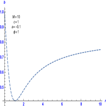
(a)

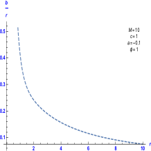
(b)

Figure 1: For $n=\frac{1}{2}$. Left plot: shape function $b$ versus $r$. Right plot: $\frac{b}{r}$ versus $r$.

From the above calculations, it is evident that the considered Lorentz distribution of a particle-like gravitational source is positive for smeared mass source parameter in our calculations. We also obtain the shape function $b(R)$ for different values of $n$ with respect to the modified $f(R)$ gravitational model in relation to wormhole. The redshift function $\Phi(r)$ is also assumed to be constant at all points.

From Fig. 1(a), it is obvious that the shape function increases with respect to $r$. Fig. 1(b) reflects that $b/r$ takes asymptotically large value when $r\rightarrow 0$, which suggests that the asymptotically flat condition is being satisfied.

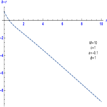
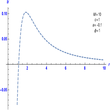
Figure 2: For $n=\frac{1}{2}$. Left plot: $b-r$ versus $r$ and right plot: $b^{\prime}$ versus $r$.

Also, one can see from the figure 2, the value of throat radius for the wormhole is estimated as $(r_{0}\approx 1)$ as curve cuts the $r$ axis at this point. Fig. 2 is plotted to check the validity of the condition $b^{\prime}(r_{0})<1$. From the plot it can be clearly seen that the corresponding condition holds. Consequently, the shape function fulfills all the requirements of warm hole structure. Figs. 3 and 3 show $\rho+P_{r}$ and $\frac{P_{r}}{\rho}$ versus $r$.

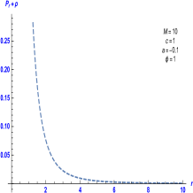
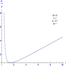
Figure 3: For $n=\frac{1}{2}$. Left plot: $\rho+P_{r}$ versus $r$. Right plot: $\frac{P_{r}}{\rho}$ versus $r$.

The radial pressure and transverse pressure are also plotted in Fig. 4 and Fig. 5, respectively. We see here that radial pressure is negative and transverse pressure is positive. Here, we note that
(a) NEC is satisfied if $\rho+P_{r}\geq 0$ and $\rho+P_{t}\geq 0$;
(b) weak energy condition (WEC) is satisfied if $\rho\geq 0$, $\rho+P_{r}\geq 0$ and $\rho+P_{t}\geq 0$;
(c) strong energy condition (SEC) is validated if $\rho+P_{r}\geq 0$ , $\rho+P_{t}\geq 0$ and $\rho+P_{r}+2P_{t}\geq 0$.
The equation of state $\omega$ in terms of radial pressure is given by $P_{r}=\omega\rho$ and the anisotropy parameter $\Delta$ is defined by $P_{t}-P_{r}$. The satisfaction and violation of the energy condition are depicted in Figs. 3, 4 and 5. The behavior of equation of state and anisotropy parameter can be seen from Figs. 3 and 6, respectively.

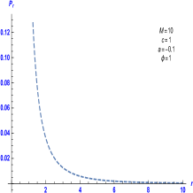
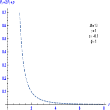
Figure 4: For $n=\frac{1}{2}$. Left plot: $P_{r}$ versus $r$. Right plot: and ($\rho+P_{r}+2P_{t}$) versus $r$.

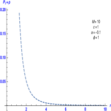
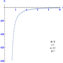
Figure 5: For $n=\frac{1}{2}$. Left plot: $\rho+P_{t}$ versus $r$. Right plot: $P_{t}$ versus $r$.

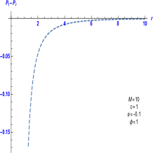
Figure 6: For $n=\frac{1}{2}$. Plot: $P_{t}-P_{r}$ versus $r$.

3.2 Negative linear model

In the case of $n=1$, we have $f(R)=-\frac{R}{2}+a$ which is a negative linear term. So, we calculate shape function for $n=1$ case as following,

$$b(r)=\frac{Mr\sqrt{\phi}}{\pi^{2}(r^{2}+\phi)}-\frac{M\arctan(\frac{r}{\sqrt{\phi}})a}{\pi^{2}}+c,$$ (3.7)

where $c$ is an integration constant. The expression of curvature scalar ($R$) for this case is given by,

$$R(r)=-\frac{2M\sqrt{\phi}((1+a)r^{2}+(-1+a)\phi)}{\pi^{2}r^{2}(r^{2}+\phi)^{2}}.$$ (3.8)

Exploiting expressions (2.8) and (3.7), the radial pressure and tangential pressure are given, respectively, by

$$P_{r} = \frac{c+\frac{Mr\sqrt{\phi}}{\pi^{2}(r^{2}+\phi)}-\frac{aM\arctan(\frac{r}{\sqrt{\phi}})}{\pi^{2}}}{2r^{3}},$$ (3.9)

$$P_{t} = \frac{c+\frac{Mr\sqrt{\phi}(a\phi+(2+a)r^{2})}{\pi^{2}(r^{2}+\phi)^{2}}-\frac{aM\arctan(\frac{r}{\sqrt{\phi}})}{\pi^{2}}}{4r^{3}}.$$ (3.10)

After having the required expressions for the case of $n=1$, we can analyze the results by plotting graphs.
For this case, in contrast to the previous case, we observe that the shape function is a decreasing function of $r$ as depicted in Fig. 7. Also, behavior of $\frac{b}{r}$ illustrated by Fig. 7.

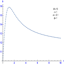
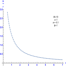
Figure 7: For $n=1$. Left side: $b$ versus $r$. Right side: $\frac{b}{r}$ versus $r$.

In Fig. 8, we draw $b-r$ versus $r$ to show that is decreasing function of radius. From Fig. 8, we see that $b^{\prime}$ takes only negative values but still follows $b^{\prime}<1$ condition.

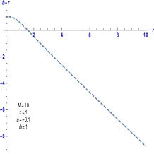
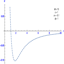
Figure 8: For $n=1$. Left side: $b-r$ versus $r$. Right side: $b^{\prime}$ versus $r$.

We draw $\rho+P_{r}$ versus $r$ by Fig. 9 and show that is decreasing function of $r$. From Fig. 9, we see that the equation of state shows opposite behavior to that of the previous case.

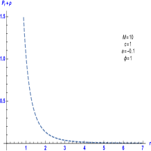
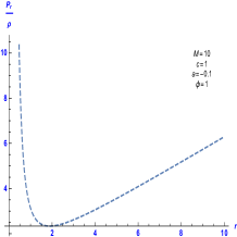
Figure 9: For $n=1$. Left plot: $\rho+P_{r}$ versus $r$. Right plot: $\frac{P_{r}}{\rho}$ versus $r$.

Also, from Figs. 10 and 11, we find that the radial pressure ($P_{r}$) and the transverse pressure ($P_{t}$) are showing opposite behavior as to the case of $n=\frac{1}{2}$. On the other hand, from Figs. 10 and 11, we see some damping periodic behavior for $\rho+P_{r}+2P_{t}$ and $\rho+P_{t}$ respectively.

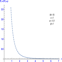
Figure 10: For $n=1$. Left plot: $P_{r}$ versus $r$. Right plot: $\rho+P_{r}+2P_{t}$ versus $r$.

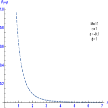
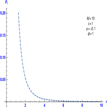
Figure 11: For $n=1$. Left plot: $\rho+P_{t}$ versus $r$. Right plot: $P_{t}$ versus $r$.

The NEC, WEC and SEC as mentioned in the previous subsection can also be studied in this case also. The anisotropy parameter in this case take negative values only as depicted from 12.

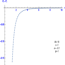
Figure 12: For $n=1$. Plot: $P_{t}-P_{r}$ versus $r$.

3.3 Squared plus negative linear model

In this part, we investigate another component of the modified $f(R)$ gravitational model, namely $n=0$, which yield $f(R)=-\frac{R}{2}+aR^{2}$. The computational process of this part is exactly the same as the previous two parts, but we deal with complicated equations which have not analytical solutions. The shape function can be obtained by using the equations (2.7), (3.1) and (3.2). We obtain the values related to curvature scalar $R$, the radial pressure $P_{r}$, tangential pressure $P_{t}$ by using the numerical calculations for the shape function $b(r)$ with respect to equations (2.6) and (2.8). The remarkable thing about this modified $f(R)$ gravitational model is that we can obtain two independent solutions for the shape function $b(r)$ corresponding $n=0$. Here, we discuss the calculations associated with each value separately. For each case, the results will be fully described along with the location of the wormhole throat and the satisfaction/ violation of the energy conditions.

3.3.1 The first numerical solutions

For this case, we observe that shape function is an increasing function of $r$ as shown in Fig. 13. From Fig. 13, we find that $b/r$ takes asymptotically large value for small $r$ and asymptotically flat condition is being satisfied.

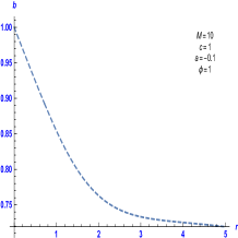
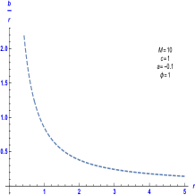
Figure 13: For $n=0$. Left plot: $b$ versus $r$. Right plot: $\frac{b}{r}$ versus $r$.

From Fig. 14, we see that two throat radii exist for wormhole. Also, from Fig. 14, we see that the shape function does not satisfy the required condition $b^{\prime}<1$.

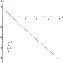
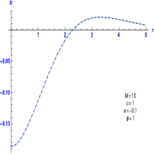
Figure 14: For $n=0$. Left plot: $b-r$ versus $r$. Right plot: $b^{\prime}$ versus $r$.

Fig. 15 $\rho+P_{r}$ versus $r$ shows that there is a minimum at small radii. From Fig. 15, we see that the equation of state shows different behavior to the previous two cases.

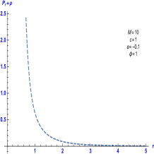
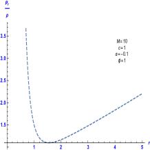
Figure 15: For $n=0$. Left plot: $\rho+P_{r}$ versus $r$. Right plot: $\frac{P_{r}}{\rho}$ versus $r$.

In the plots 16 and 17, we can see that the radial pressure ($P_{r}$) and the transverse pressure ($P_{t}$) are showing opposite behavior. The region where NEC, WEC and SEC are satisfied/violated can be studied from the plots 15, 16 and 17. The $\rho+P_{r}$ and $\rho+P_{r}+2P_{t}$ showing similar behavior in contrast to above cases.

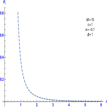
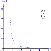
Figure 16: For $n=0$. Left plot: $P_{r}$ versus $r$. Right plot: $\rho+P_{r}+2P_{t}$ versus $r$.

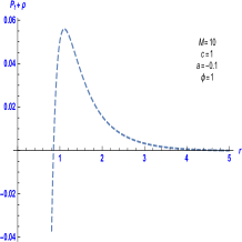
Figure 17: For $n=0$. Left plot: $\rho+P_{t}$ versus $r$. Right plot: $P_{t}$ versus $r$.

Anisotropy parameter curve shows behavior like nuclear potential as depicted in Fig. 18, which including a minimum at small radii.

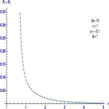
Figure 18: For $n=0$. Plot: $P_{t}-P_{r}$ versus $r$.

3.3.2 The second numerical solutions

In the second case of $n=0$, on the contrary, we observe that shape function is a decreasing function of $r$ as shown in Fig. 19. From Fig. 19, we find that $b/r$ takes asymptotically large value for small $r$ and asymptotically flat condition is being satisfied here also.

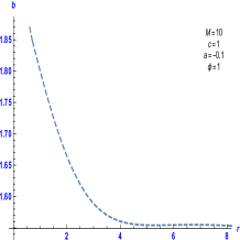
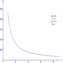
Figure 19: For $n=0$. Left plot: $b$ versus $r$. Right plot: $\frac{b}{r}$ versus $r$.

From Fig. 20, we see that the throat radius take value $r\approx 1$ for wormhole. Moreover, from Fig. 20, we see that the shape function satisfies the required condition $b^{\prime}<1$.

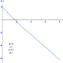
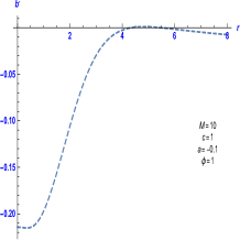
Figure 20: For $n=0$. Left plot: $b-r$ versus $r$. Right plot: $b^{\prime}$ versus $r$.

From 21, we see that the equation of state takes asymptotically small value for small $r$. In the plots 22 and 23, we can see that the radial pressure ($P_{r}$) and the transverse pressure ($P_{t}$) show opposite nature to the first case of $n=0$. Anisotropy parameter curve shows similar behavior of equation of state as depicted in figure 24. The region where NEC, WEC and SEC are satisfied/violated can be studied from the plots 21, 22 and 23. The $\rho+P_{r}$ and $\rho+P_{r}+2P_{t}$ showing similar behavior in contrast to $n=1/2,1$ cases.

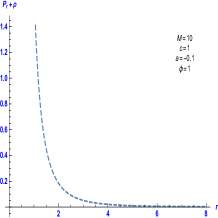
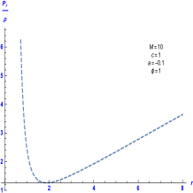
Figure 21: For $n=0$. Left plot: $\rho+P_{r}$ versus $r$. Right plot: $\frac{P_{r}}{\rho}$ versus $r$.

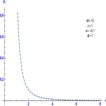
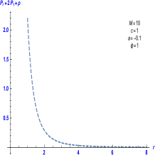
Figure 22: For $n=0$. Left plot: $P_{r}$ versus $r$. Right plot: $\rho+P_{r}+2P_{t}$ versus $r$.

Figure 23: For $n=0$. Left plot: $\rho+P_{t}$ versus $r$. Right plot: $P_{t}$ versus $r$.

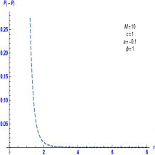
Figure 24: For $n=0$. Plot: $P_{t}-P_{r}$ versus $r$.

We end up this section by stating that these concepts expressed here can be applied to other models as well. The more interesting point here is that by introducing different wormholes and recently proposed conditions such as weak gravity conjecture, one can shed new light on the structure associated with wormholes.

At the end of this section, the energy conditions for different $n$ for this model can be briefly expressed in the following form.
$\bullet$ for $n=\frac{1}{2}$, $NEC$, $WEC$, and $SEC$ are satisfied.
$\bullet$ for $n=1$, $NEC$, $WEC$, and $SEC$ are satisfied.
$\bullet$ for $n=0(I)$ , $NEC$, $WEC$, and $SEC$ are satisfied in $(r>1)$
$\bullet$ for $n=0(II)$ , $NEC$, $WEC$, and $SEC$ are satisfied

4 Specific solutions for the power law model

In this section, we consider another model where $f(R)$ specifies as[47, 48, 49, 50]

$$f(R)=\frac{\alpha}{R^{n}},$$ (4.1)

where $\alpha$ and $n$ are some constants. In fact, our main goal is to obtain the field equations using non-commutative geometry with Lorentzian distribution. So, we express the energy density $(\rho)$ associated with spherical symmetry and particle-like gravitational source Which is mentioned in equation (3.2)[38]: Now, with respect to equations (2.6) and (4.1) we have

$$f(R)=\frac{\alpha}{\left(2\frac{b^{\prime}}{r^{2}}\right)^{n}}.$$ (4.2)

Now by plugging expression (3.2) and (4.2) in equation (2.7), we obtain the shape function $b(r)$ given by

$$b(r)=\int\pi^{\frac{2}{n-1}}\left(\frac{2^{n}M(\frac{1}{r^{2}})^{n-1}\sqrt{\phi}}{\alpha(r^{2}+\phi)^{2}}\right)^{\frac{1}{n-1}}dr.$$ (4.3)

Then, we shall study the specific cases corresponding to different values of $n$.

4.1 Shape function, energy condition and equation of states for $n=\frac{1}{2}$

For $n=\frac{1}{2}$, the shape function (4.3) simplifies to

$$b(r)=\frac{M^{2}}{24\alpha^{2}\pi^{4}\phi^{\frac{3}{2}}}\left[-\frac{\sqrt{\phi}r(\phi-3r^{2})(3\phi+r^{2})}{(\phi+r^{2})^{3}}+3\arctan\left(\frac{r}{\sqrt{\phi}}\right)\right]+c,$$ (4.4)

where $c$ is an integration constant.

Utilizing expressions (4.4) and (2.6), we obtain the specific form of curvature scalar as following:

$$R(r)=\frac{4M^{2}\phi}{\alpha^{2}\pi^{4}(\phi+r^{2}){4}}$$ (4.5)

With the help of expressions (4.4) and (2.8), the radial pressure and tangential pressure are computed, respectively, as

$$P_{r} = \frac{A}{B},$$ (4.6)

$$A = -\alpha\sqrt{\frac{M^{2}\phi^{2}}{\alpha^{2}(\phi+r^{2})^{4}}}\left(-\sqrt{\phi}(24\alpha^{2}c\pi^{4}\phi(\phi+r^{2})^{4}+M^{2}r(-\phi+r^{2})(3\phi^{2}+14\phi r^{2}+3r^{4})\right)$$ (4.7)

$$- 3M^{2}(\phi+r^{2})^{4}\arctan(\frac{r}{\sqrt{\phi}}),$$

$$B = 32M^{2}\pi^{2}\phi^{\frac{5}{2}}r^{3},$$ (4.8)

$$P_{t} = \frac{C}{D},$$ (4.9)

$$C = -\alpha\sqrt{\frac{M^{2}\phi}{\alpha^{2}(\phi+r^{2})^{4}}}(-\sqrt{\phi}r(16\alpha^{2}\pi^{4}\phi)(\phi+r^{2})^{4}+M^{2}(\phi-r^{2})$$ (4.10)

$$\times(3\phi^{2}+14\phi r^{2}+3r^{4})-3M^{2}(\phi+r^{2})^{4}\arctan(\frac{r}{\sqrt{\phi}})),$$

$$D = 32\pi^{2}M^{2}\phi^{\frac{5}{2}}r^{3}.$$ (4.11)

Now, to analyze these results, we plot graphs.

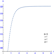
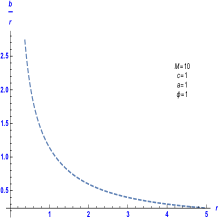
Figure 25: For $n=\frac{1}{2}$. Left plot: $b$ versus $r$. Right plot: $\frac{b}{r}$ versus $r$.

From Fig. LABEL:25a, it is obvious that the shape function increases rapidly and saturates after a point along with $r$. In Fig. LABEL:25b, we see that similar to other cases here also $b/r$ takes asymptotically large value when $r\rightarrow 0$, which suggests that the asymptotically flat condition is being satisfied.
In this case of $f(R)$ model, the value of throat radius for the wormhole in this model is $(r_{0}\approx 1.2)$ as depicted in the figure 26. In Fig. 26, justifies the validity of the condition $b^{\prime}(r_{0})<1$ and, hence, the shape function satisfies all the requirements of warm hole structure.

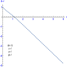
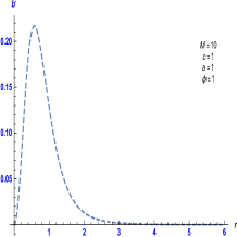
Figure 26: For $n=\frac{1}{2}$. Left plot: $b-r$ versus $r$. Right plot: $b^{\prime}$ versus $r$.

We draw $\rho+P_{r}$ versus $r$ in Figs. 27. The radial pressure plotted in Figs. 27. We see here that radial pressure is negative as well as $\rho+P_{r}$.

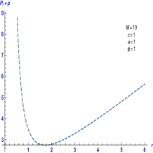
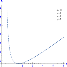
Figure 27: For $n=\frac{1}{2}$. Left plot: $\rho+P_{r}$ versus $r$. Right plot: $P_{r}$ versus $r$.

The satisfaction and violation of the energy condition are depicted in Figs. 27, 28 and 29. The transverse pressure is also plotted in Figs. 29, to see that transverse pressure has both positive and negative values.

The behavior of equation of state and anisotropy parameter can be seen from Figs. 28 and 30, respectively.

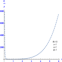
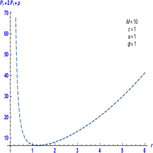
Figure 28: For $n=\frac{1}{2}$. Left plot: $\frac{P_{r}}{\rho}$ versus $r$. Right plot: $\rho+P_{r}+2P_{t}$ versus $r$.

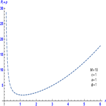
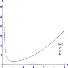
Figure 29: For $n=\frac{1}{2}$. Left plot: $\rho+P_{t}$ versus $r$. Right plot: $P_{t}$ versus $r$.

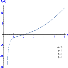
Figure 30: For $n=\frac{1}{2}$. Plot: $P_{t}-P_{r}$ versus $r$.

In the upcoming subsections, we shall study the other components of modified $f(R)$ gravity, namely, $n=\frac{3}{2}$ and $n=\frac{1}{10}$. One can see the effect of different value of $n$ on location of the wormhole throat and also radial pressure $P_{r}$ and transverse pressure ($P_{t}$) as well as the different energy conditions corresponding to NEC, WEC and SEC.

4.2 Shape function, energy condition and equation of states for $n=\frac{9}{10}$

In the case of $n=\frac{9}{10}$, we obtain the following value of shape function:

$$b(r)=1.94604\times 10^{-8}r(\frac{M\sqrt{\phi}}{\alpha(\frac{1}{r^{2}})^{\frac{1}{10}}(\phi+r^{2})^{2}})^{10}(1+\frac{r^{2}}{\phi})^{20}\mathcal{H}\bigg{[}1.5,20,2.5,-\frac{1.1r^{2}}{\phi}\bigg{]},$$ (4.12)

where $\mathcal{H}$ is Hypergeometric ${}_{2}F_{1}$ function. Now, like the previous parts we study the energy condition for this model by plotting graphs. From Fig. 31, one can see that the shape function is an increasing function of $r$ and takes infinitesimally small for small $r$. In Fig. 31, we see that $b/r$ takes only positive value and becomes asymptotically large when $r\rightarrow 0$ as well as $r>1.5$.

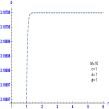
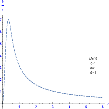
Figure 31: For $n=\frac{9}{10}$. Left plot: $b$ versus $r$. Right plot: $\frac{b}{r}$ versus $r$.

In Fig. 32, we observe that $b-r$ cut the $r$-axis but approaches very closely around $r=3$. Fig. 32 justifies the violation of validity of the condition $b^{\prime}(r_{0})<1$. This suggests that the shape function does not satisfy all the requirements of warm hole structure.

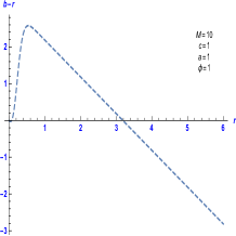
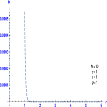
Figure 32: For $n=\frac{9}{10}$. Left plot: $b-r$ versus $r$. Right plot: $b^{\prime}$ versus $r$.

The radial pressure and transverse pressure are also plotted in figures 33 and 35, respectively. Here, we see that the radial pressure and transverse pressure both have asymptotically positive value when $r\rightarrow 0$. However, for large $r$ both takes very small values but of opposite nature. The satisfaction and violation of different energy condition are depicted in Figs. 33, 34 and 35. The Fig. 34 suggests that equation of state becomes negative for small values of $r$ and and takes asymptotically large value when $r\rightarrow 0$. The anisotropy parameter is plotted in 36. The plot shows that $P_{t}$ dominates over $P_{r}$.

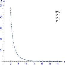
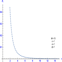
Figure 33: For $n=\frac{9}{10}$. Left plot: $\rho+P_{r}$ versus $r$. Right plot: $P_{r}$ versus $r$.

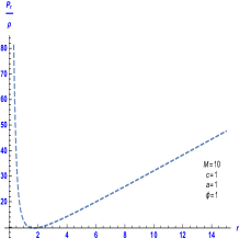
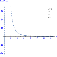
Figure 34: For $n=\frac{9}{10}$. Left plot: $\frac{P_{r}}{\rho}$ versus $r$. Right plot: $\rho+P_{r}+2P_{t}$ versus $r$.

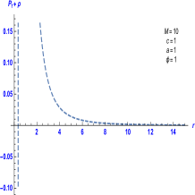
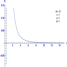
Figure 35: For $n=\frac{9}{10}$. Left plot: $\rho+P_{t}$ versus $r$. Right plot: $P_{t}$ versus $r$.

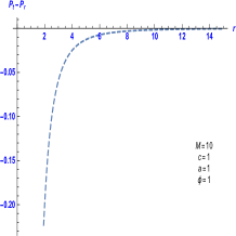
Figure 36: For $n=\frac{9}{10}$. Plot: $P_{t}-P_{r}$ versus $r$.

4.3 Shape function, energy condition and equation of states for $n=\frac{1}{10}$

We start this subsection by writing the shape function for the case of $f(R)$ gravity for $n=0.1$ as follows

$$b(r)=0.03r\left[\frac{M\sqrt{\phi}}{\alpha(\frac{1}{r^{2}})^{0.9}}(r^{2}+\phi)^{2}\right]^{1.1}\left(1+\frac{r^{2}}{\phi}\right)^{2.22}{}_{2}F_{1}\left[1.5,2.22,2.5,-\frac{r^{2}}{\phi}\right]+c.$$ (4.13)

By plugging this value of shape function in (2.6), one can obtained the curvature scalar ($R$). It is difficult to solve the other equations numerically as the shape function contains hypergeometric function. So, we try to describe the results by plotting some figures as following.

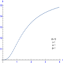
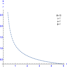
Figure 37: For $n=\frac{1}{10}$. Left plot: $b$ versus $r$. Right plot: $\frac{b}{r}$ versus $r$.

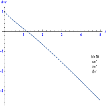
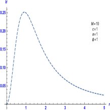
Figure 38: For $n=\frac{1}{10}$. Left plot: $b-r$ versus $r$. Right plot: $b^{\prime}$ versus $r$.

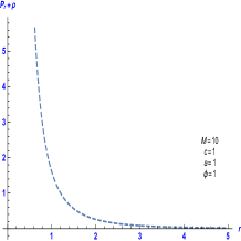
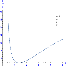
Figure 39: For $n=\frac{1}{10}$. Left plot: $\rho+P_{r}$ versus $r$. Right plot: $\frac{P_{r}}{\rho}$ versus $r$.

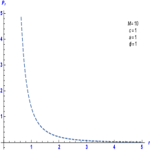
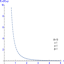
Figure 40: For $n=\frac{1}{10}$. Left plot: $P_{r}$ versus $r$. Right plot: $\rho+P_{r}+2P_{t}$ versus $r$.

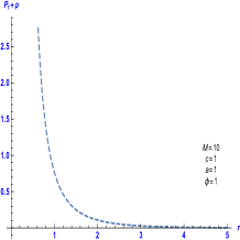
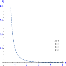
Figure 41: For $n=\frac{1}{10}$. Left plot: $\rho+P_{t}$ versus $r$. Right plot: $P_{t}$ versus $r$.

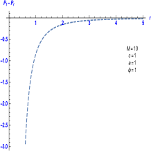
Figure 42: For $n=\frac{1}{10}$. Plot $P_{t}-P_{r}$ versus $r$.

From Fig. 37, one can see that the shape function is an increasing function of $r$ and and depends on $r$ more or less linearly. Fig. 37 confirms that asymptotically flat condition is being satisfied. In the figure 38, we observe that $b-r$ curve cuts the $r$-axis around $r=1.2$ which confirms the value of throat radius in this case. From the Fig. 38, we observe that the validity of the condition $b^{\prime}(r_{0})<1$ holds and therefore the shape function satisfies all the requirements of warm hole structure. The radial pressure is plotted in figure 40, which confirms that the radial pressure takes asymptotically negative value when $r\rightarrow 0$ and takes zero value for large $r$. The transverse pressure is plotted in figure 41. Plot suggests that transverse pressure is just negative to that of radial pressure. The satisfaction and violation of different energy condition are depicted in Figs. 39, 40 and 41. The behavior of equation of state can be seen from Fig. 39. The anisotropy parameter is plotted in 42 which shows that $P_{t}$ is a decreasing function of $r$ and dominates over $P_{r}$. The important point in examining the two models in this paper is that problems arise for the energy condition for the first model in (n=0), i.e., SEC. Still, for certain values of r, energy conditions are fully established. Also, for the second model, the energy conditions in the range $0<n<1$ are well established, but when I consider ($n=0$), the wormhole throat and energy conditions have problems. Also, as we get closer to 1, both the wormhole throat and the energy conditions are accompanied by problems. From $0<n<1/2$, the energy conditions are favorable. When we are moving forward the values as $n>1/2$, the problems gradually occur, i.e., the energy conditions are no longer established for certain $r$.

At the end of this section, the energy conditions for different $n$ for this model can be briefly expressed in the following form.
$\bullet$ for $n=\frac{1}{2}$, $NEC$, $WEC$, and $SEC$ are satisfied.
$\bullet$ for $n=\frac{9}{10}$, $NEC$, $WEC$, and $SEC$ are satisfied in $n\gtrapprox 1$ .
$\bullet$ for $n=\frac{1}{10}$ , $NEC$, $WEC$, and $SEC$ are satisfied

We end up this section by commenting that different conditions corresponding to different energy conditions were examined by determining the shape function for the modified $f(R)$ gravitational model. The results are interesting as the energy condition and validity of shape function depends on the value of $n$ in the particular choice of the model. So, the results can be used in searching appropriate modified $f(R)$ model for wormhole.

5 Concluding remarks

It is known that wormholes are a series of imaginary objects whose geometry can solve Einstein equations by tolerating the violation of NEC. In the recent past, researchers have studied diverse wormholes according to different criteria, and they achieved elegance, bizarre, and exciting results that may be able to solve many mysteries. Keeping this in mind, we have investigated a series of exact solutions for a static wormhole following smeared mass source geometry in the modified $f(R)$ gravitational model where Lorentzian distribution resulting from a particle-like source has been considered. In particular, we have studied two particular models of modified $f(R)$ gravity model and have analyzed the results corresponding to different cases of these models. We have first derived shape function for different values of $n$ in both the $f(R)$ models. From the shape function, we have calculated the scalar curvature, radial pressure and transverse pressure. Furthermore, we have studied the behavior of quantities by plotting the graph and validity of different energy condition, in particular, NEC, WEC and SEC. The energy of state and anisotropy parameter have also been emphasized for each case. From the plots, we can estimate the value of throat radius for the wormhole. Remarkable, we have found that for $n=0$, there exist two shape functions showing different behavior. The results are really interesting which can be useful in exploring a suitable model for wormhole. It will be interesting to study further the wormhole under different conditions. Also, it is interesting to consider some corrections on $f(R)$ like logarithmic correction [44] or use $f(R,L)$ theories [45].

References

- [1] L. Flamm, Physik Z. 17, 448 (1916).
- [2] A. Einstein and N. Rosen, Ann. Phys. 242, 2 (1935).
- [3] I. D. Novikov, A.A. Shatskiy and D. I. Novikov, [arXiv:1412.3749].
- [4] J. Maldacena, A. Milekhin, F. Popov, [arXiv:1807.04726].
- [5] J. L. Blazquez-Salcedo, C. Knoll, E. Radu, [arXiv:2010.07317].
- [6] E. Teo, Phys. Rev. D 58 024014 (1998).
- [7] P. K. F. Kuhfittig, Phys. Rev. D 67, 064015 (2003).
- [8] P. E. Kashargin and S.V. Sushkov, Grav. Cosmol. 14, 80 (2008).
- [9] M. Jamil, P. K. F. Kuhfittig, F. Rahaman and S. A Rakib, Eur. Phys. J. C 67, 513 (2010).
- [10] G. Clement, Phys. Rev. D 51 6803 (1995).
- [11] J. P. S. Lemos et al, Phys. Rev. D 68 064004 (2003).
- [12] F. Rahaman et al, Gen. Rel. Grav. 39 145 (2007).
- [13] J. P. S. Lemos and F. S. N. Lobo, Phys. Rev. D 78, 044030 (2008).
- [14] F. Rahaman et. al, Gen. Rel. Grav. 38, 1687 (2006).
- [15] F. Rahaman et. al, Mod. Phys. Lett. A24, 53 (2009).
- [16] F. Rahaman et. al, Class. Quant. Grav. 28, 155021 (2011).
- [17] F. Rahaman et .al, Int. J. Theor. Phys. 51, 1680(2012).
- [18] S.-W. Kim and H. Lee, Phys. Rev. D 63, 064014 (2001).
- [19] F. Rahaman et. al, Int. J. Theor. Phys. 48, 1637 (2009).
- [20] F. S. N. Lobo, Classical and Quantum Gravity Research, 1-78 (2008), Nova Sci. Pub.
- [21] M. S. Morris and K. S. Thorne, Am. J. Phys. 56, 395 (1988).
- [22] M. S. Morris et. al, Phys. Rev. Lett. 61, 1446 (1988).
- [23] T. A. Roman, Phys. Rev. D 47, 1370 (1993).
- [24] S. W. Hawking, Phys. Rev. D 46, 603(1992).
- [25] F. Rahaman, S. Sarkar, K. N. Singh and N. Pant, Mod. Phys. Lett. A 34, 1950010 (2019).
- [26] N. Godani and G. C. Samanta, Mod. Phys. Lett. A 34, 1950226 (2019).
- [27] N. Godani and G. C. Samanta, New Astron. 80, 101399 (2020).
- [28] N. Godani and G. C. Samanta, Eur. Phys. J. C 80, 30 (2020).
- [29] G. C. Samanta and N. Godani, Eur. Phys. J. C 79, 623 (2019).
- [30] O. L. Andino and C. L. Vasconez, [arxiv:2007.10422].
- [31] N. Sorokhaibam, [arxiv:2007.07169].
- [32] P. K. F. Kuhfittig, J. Appl. Math. and Phys. 8, 1263 (2020).
- [33] A. C. L. Santos, C. R. Muniz and L. T. Oliveira, [arxiv:2007.00227].
- [34] M. Chernicoff, E. Garcia, G. Giribet and E. Rubin de Celis, JHEP 2020, 19 (2020) [arxiv:2006.07428].
- [35] C. X. Yan, T. Gansukh and Y. D.-han, [arxiv:2006.04344].
- [36] I. Fayyaz and M. F. Shamir, Eur. Phys. J. C 80, 430 (2020).
- [37] F. S. N. Lobo and M. A. Oliveira, Phys. Rev. D 80, 104012 (2009).
- [38] S. H. Mehdipour, Eur. Phys. J. Plus 127, 80 (2012).; F. Rahaman et al., Phys. Rev. D 86, 106010 (2012); F. Rahaman et al., Phys. Lett. B 746, 73 (2015); F. Rahaman et al., Int. J. Theor. Phys. 54, 699 (2015).
- [39] M. Khurshudyan, B. Pourhassan, A. Pasqua, Can. J. Phys. 93, 449 (2015).
- [40] S. Capozziello, M. Faizal, M. Hameeda, B. Pourhassan, V. Salzano, S. Upadhyay, MNRAS 474, 2430 (2018)
- [41] O. Bertolami et. al, Phys. Rev. D 75, 104016. (2007).
- [42] M. Rostami, J. Sadeghi, S. Miraboutalebi, A. A. Masoudi, B. Pourhassan, Int. J. Geom. Meth. Mod. Phys. 17, 2050136 (2020).
- [43] M., Cataldo, et al., Phys. Rev. D 79, 024005 (2009).
- [44] J. Sadeghi, B. Pourhassan, A.S. Kubeka, M. Rostami, Int. J. Mod. Phys. D 25, 1650077 (2016).
- [45] B. Pourhassan and P. Rudra, Phys. Rev. D 101, 084057 (2020).
- [46] Phongpichit Channuie, arXiv:1907.10605 (2019).
- [47] L. Sebastiani, G. Cognola, R. Myrzakulov, S. D. Odintsov and S. Zerbini, Phys. Rev. D 89 2, 023518 (2014).
- [48] R. Myrzakulov, S. Odintsov and L. Sebastiani, Phys. Rev. D 91 8, 083529 (2015).
- [49] K. Bamba, R. Myrzakulov, S. D. Odintsov and L. Sebastiani, Phys. Rev. D 90 4, 043505 (2014).
- [50] A. Codello, J. Joergensen, F. Sannino and O. Svendsen, JHEP 1502 050(2015).