Fast Road Segmentation via Uncertainty-aware Symmetric Network

Abstract

The high performance of RGB-D based road segmentation methods contrasts with their rare application in commercial autonomous driving, which is owing to two reasons: 1) the prior methods cannot achieve high inference speed and high accuracy in both ways; 2) the different properties of RGB and depth data are not well-exploited, limiting the reliability of predicted road. In this paper, based on the evidence theory, an uncertainty-aware symmetric network (USNet) is proposed to achieve a trade-off between speed and accuracy by fully fusing RGB and depth data. Firstly, cross-modal feature fusion operations, which are indispensable in the prior RGB-D based methods, are abandoned. We instead separately adopt two light-weight subnetworks to learn road representations from RGB and depth inputs. The light-weight structure guarantees the real-time inference of our method. Moreover, a multi-scale evidence collection (MEC) module is designed to collect evidence in multiple scales for each modality, which provides sufficient evidence for pixel class determination. Finally, in uncertainty-aware fusion (UAF) module, the uncertainty of each modality is perceived to guide the fusion of the two subnetworks. Experimental results demonstrate that our method achieves a state-of-the-art accuracy with real-time inference speed of 43+ FPS. The source code is available at https://github.com/morancyc/USNet.

I INTRODUCTION

Road segmentation aims to classify each pixel of an image as drivable or undrivable and provides the drivable region to other modules in self-driving system for safe navigation. Obviously, both high efficiency and reliability are necessary for road segmentation. In recent years, many algorithms have been proposed to segment road based on vision sensors, i.e., 3D LiDAR, monocular and stereo camera. Compared to the works using low-cost monocular [1, 2, 3] and expensive LiDAR sensors [4, 5, 6], the road segmentation methods using affordable stereo camera [7, 8, 9], namely RGB-D based methods, achieve a better trade-off between cost and reliability. Thus, they are valued by the community recently.

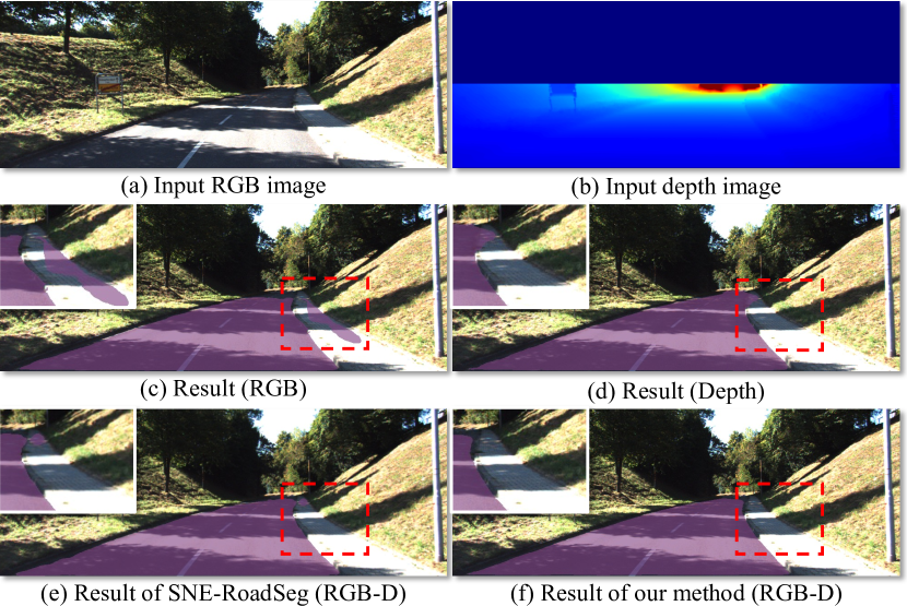
Figure 1: Segmentation results of different models. (a) RGB image. (b) Depth image. (c) Result of the model using RGB as input. (d) Result of the model using Depth as input. (e) Result of SNE-RoadSeg [7]. (f) Result of our method. The segmented road are marked in purple, and the images are zoomed to clearly show the details.

However, the prevalence of RGB-D based methods contrasts with their rare application. One of the reasons is that although a great breakthrough in performance has been made, the previous RGB-D based road segmentation methods still cannot run in real-time. Another reason is that the previous methods are limited on the reliability of predicted road, as they cannot fully utilize the particular characteristics of RGB and depth data. Theoretically, RGB and depth data are two basic visual modalities that express the 2D space and 3D space, respectively. They hold different characteristics: RGB data is sensitive to light-dark contrast in the 2D spatial domain, while depth data is sensitive to distance change in the 3D spatial domain. How to perceive the characteristic difference is a key issue for RGB-D based road segmentation. The previous methods [7, 8, 9] commonly merge RGB and depth data by summing features of the two modalities to form a unified representation of road. However, RGB and depth features are indiscriminately fused in this design, bringing in conflict of feature representation in the sensitive region of RGB and depth data. It would lead to wrong segmentation inside these sensitive regions. To better explain this issue, we trained two networks that utilize RGB and depth image as input respectively. As shown in Fig.1 (c) (d), the RGB-based and depth-based models show different false positives, which are caused by their different representations of the road. This conflict cannot be eliminated by adding the two modality features [7], as shown in Fig.1 (e).

To address this issue, we abandon the mainstream idea of boosting the discriminative power of features adopted by many works [10, 11, 12, 13, 14] on other vision tasks. In this paper, we introduce evidence theory to fuse RGB and depth data and gain state-of-the-art performance with low computational cost. To this end, an uncertainty-aware symmetric network (USNet) is proposed, which perceives the uncertainties of each modality, and incorporates the uncertainties into the fusion process. Firstly, the cross-modal feature fusion utilized by previous works [7, 8, 9] is abandoned. We instead design two light-weight subnetworks to learn road representations from RGB and depth inputs, avoiding feature-level conflict. Secondly, for each modality, a multi-scale evidence collection (MEC) module is proposed to collect evidence of a pixel belonging to road or non-road in multiple scales. Thirdly, based on the evidence given by the two subnetworks, an uncertainty-aware fusion (UAF) module is designed to perceive the uncertainty of each modality, and determine the probability and uncertainty that a pixel belongs to road or non-road. In practical application, the perceived uncertainty can be provided to the self-driving system for further obstacle discovery [15, 16]. As shown in Fig. 1 (f), by considering the uncertainty of each modality, our method eliminates the wrong segmentation completely. Our network achieves comparable performance with the state-of-the-art methods with an inference speed of 43$+$ FPS, 4$\times$$\sim$10$\times$ faster than the former state-of-the-art methods. The contributions of our approach lie in:

• The conflict of RGB and depth data in feature space is revealed, which guides us to propose a light-weight symmetric paradigm for RGB-D based road segmentation to avoid the feature conflict of different modalities.

• Based on the evidence theory, a multi-scale evidence collection (MEC) module is proposed to obtain sufficient evidence of road and non-road, so that the well-designed uncertainty-aware fusion (UAF) module makes full use of the characteristics of RGB and depth data.

• Our method gains state-of-the-art accuracy on both the KITTI benchmark [17] and the Cityscapes dataset [18], while with a low cost of computation and parameter.

II Related Work

II-A Road Segmentation

Road segmentation has been studied for decades. It is vital in self-driving and mobile robot applications [19, 20]. After Long et al. [21] proposed the pioneering work, i.e., Fully Convolutional Network (FCN), for semantic segmentation, many methods based on the FCN framework have arisen. Previous methods can be divided into three groups: RGB-based methods [22, 23], RGB-LiDAR based methods [4, 5], and RGB-D based methods [7, 9, 24].

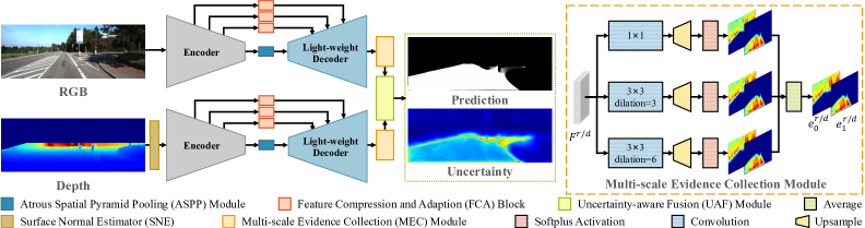
Figure 2: Network architecture of USNet. It uses SNE [7] to calculate the surface normal. Our network is composed of two subnetworks that take RGB and depth image as input, respectively. The detailed structure of the multi-scale evidence collection (MEC) module is shown in the right.

The RGB-based methods [2, 3] improve the accuracy of road segmentation by introducing extra cue, such as boundary [25, 13] and object [26, 27]. However, they may fail when there exist illumination variations in the RGB image. Considering the above problem, many approaches use LiDAR or Depth data as a supplement [4, 5, 24]. As for the RGB-D based methods, Wang et al. [24] propose an effective and efficient data-fusion strategy named DFM to fuse RGB and depth features. Based on the hypothesis that the road area in one image is coplanar, [7, 8, 9] propose to estimate surface normal from the depth image and utilize the surface normal as the input of the network. However, the different characteristics of RGB and depth data have not been well utilized by the above-mentioned methods, thus leaving room for performance improvement.

II-B Evidence-based Learning

Vanilla neural networks make predictions by a deterministic learning pipeline. However, accurate predictions achieved on datasets are not sufficient to cope with the real world. It is also significant to obtain the reliability of the prediction. To this end, evidence-based methods propose a way to model the uncertainty of prediction [28, 29]. The idea of evidence-based learning comes from Dempster–Shafer Theory of Evidence (DST) [30]. Subjective Logic (SL) [31] defines a framework that formalizes DST’s notion of belief assignments as a Dirichlet Distribution. Based on the SL, Sensoy et al. [28] propose a framework to model the uncertainty of classification tasks. After that, Han et al. [29] accomplish trusted classification by using Dempster’s combination rule to fuse classifications of multiple views. Inspired by [29], we follow the evidence-based fusion strategy to realize uncertainty-aware RGB-D road segmentation.

III Background

The theoretical basis of uncertainty modeling in our method is Subjective Logic (SL) [31]. In this section, we give a brief review of it.

For $K$-class classification, a front-end model is utilized to extract evidence, namely, information that supports a sample to be classified into a certain class. Based on the extracted evidence, SL assigns a probability (called belief mass) to each class, and generates an overall uncertainty (called uncertainty mass) of this assignment. The belief assignment is formalized as a Dirichlet distribution in SL, and the concentration parameters of the Dirichlet distribution are related to the evidence. To be specific, the evidence of each class is denoted as $e_{k},\ k=1,...,K$, where $e_{k}\geq 0$. And the concentration parameters $\alpha_{k}$ of this Dirichlet distribution is pre-defined as $\alpha_{k}=e_{k}+1$. Then the belief mass $b_{k}$ and the uncertainty $u$ can be computed by:

$$b_{k}=\frac{e_{k}}{S}=\frac{\alpha_{k}-1}{S}\quad and\quad u=\frac{K}{S}$$ (1)

where $S={\sum_{k=1}^{K}}(e_{k}+1)={\sum_{k=1}^{K}}\alpha_{k}$ is the Dirichlet strength. Intuitively, the uncertainty $u$ is inversely proportional to the total evidence $\sum_{k=1}^{K}e_{k}$, which means the more evidence collected, the lower the uncertainty. According to Eq. 1, the $K$ belief masses $b_{k}$ and $u$ are all non-negative and their sum is one: $u+\sum\nolimits_{k=1}^{K}b_{k}=1$. Given the belief assignment, the expected probability for the $k$-th class is the mean of the corresponding Dirichlet distribution:

$$\hat{p}_{k}=\frac{\alpha_{k}}{S}$$ (2)

In this paper, we use a CNN to collect evidence from input images, and calculate the uncertainty of each pixel to guide the fusion of predicted road from RGB and depth data.

IV METHODOLOGY

In this section, we propose an uncertainty-aware symmetric network (USNet), which is illustrated in Fig. 2. Note that, the depth image is processed by the surface normal estimator (SNE) [7] to generate a three-channel surface normal that is taken as the input for the depth subnetwork. This transformation is important for our method as it provides a more effective representation of the road. Different from the previous road segmentation methods [7, 8, 9] which conduct cross-modal feature fusion, the USNet learns two feature representations of road from RGB and depth image by two independent subnetworks (see Sec. IV-A), respectively. Then, sufficient evidence is collected from the well-designed multi-scale evidence collection (MEC) module (see Sec. IV-B). Finally, an uncertainty-aware fusion (UAF) module is introduced to determine the pixel class based on evidence of the two modalities (see Sec. IV-C).

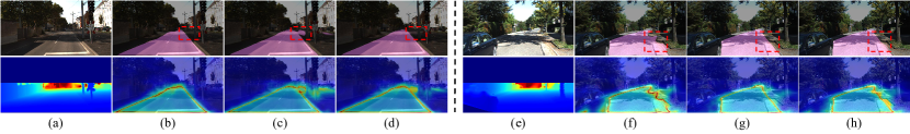
Figure 3: Visualization of uncertainty-aware fusion. (a) and (e): RGB and depth images. (b) and (f): $b_{1}^{\mathbf{r}}$ and $u^{\mathbf{r}}$ of the RGB subnetwork. (c) and (g): $b_{1}^{\mathbf{d}}$ and $u^{\mathbf{d}}$ of the depth subnetwork. (d) and (h): $b_{1}$ and $u$ after fusion. The density of the color map indicates the magnitude of value.

IV-A Unimodal Subnetwork to Obtain Road Representation

In USNet, the subnetwork for unimodal aims to extract the feature representation of road from an RGB or depth image. The subnetwork is mainly composed of an encoder and a light-weight decoder. To be specific, the ResNet-18 [32] is exploited as the encoder for low latency. At the end of the encoder, inspired by [33], an atrous spatial pyramid pooling (ASPP) module [34] is employed to perceive multi-scale context for road segmentation. Subsequently, the side-outputs of the encoder are extended by several simple blocks, called feature compression and adaptation (FCA) blocks. In an FCA block, a $1\times 1$ convolution is applied to reduce the number of channels to 64, followed by a channel-wise attention extractor [35] to enhance the discriminative channels for road representation. The FCA block helps the subnetwork to restore scene details by incorporating the compressed feature into the decoder. The decoder part of the subnetwork follows a zero-parameter structure to reduce model complexity. It consists of three upsampling-summing stages to gradually upsample the feature to $1/4$ size of the original image. Each stage straightforwardly sums the upsampled feature from the previous stage with the feature from the corresponding FCA block. Note that the first stage takes ASPP output as the input. And the last stage of the decoder yields the finest 64-channel feature. In summary, the light-weight design ensures the high inference speed of USNet.

IV-B Multi-scale Evidence Collection (MEC) Module

To sufficiently gain evidence for judging a pixel’s class, we append a multi-scale evidence collection (MEC) module after each subnetwork. The detailed structure of MEC is shown in Fig. 2. For the MEC of RGB subnetwork, given the RGB feature output by the decoder, denoted as $F^{\mathbf{r}}$, the MEC outputs two evidence maps $\{e_{0}^{\mathbf{r}},e_{1}^{\mathbf{r}}\}$, where $e_{0}^{\mathbf{r}}$ indicates the pixel-wise evidence of non-road, and $e_{1}^{\mathbf{r}}$ for that of road.

Specifically, MEC consists of three parallel paths. In each path, a convolution is first employed to gain a two-channel feature map at multiple scales. The kernel sizes of the convolution in these paths are $1\times 1$, $3\times 3$, and $3\times 3$, and the dilation rates of the two $3\times 3$ convolutions are $3$, $6$, respectively. Then, an upsample layer is employed to upscale the two-channel feature map to the size of the original image. At the end of each path, a softplus activation layer is used to realize the non-negativity of all feature values, obtaining evidence maps $\{[e_{0}^{\mathbf{r}}]^{h},[e_{1}^{\mathbf{r}}]^{h}\}$, where $h=1,2,3$ is the index of the path. Then the final evidence of the RGB subnetwork is defined as the mean of these evidence maps in all paths:

$$e^{\mathbf{r}}_{k}=\frac{1}{3}\sum\nolimits_{h=1}^{3}[e_{k}^{\mathbf{r}}]^{h},\quad k=0,1$$ (3)

For the depth subnetwork, we use another MEC to capture evidence maps $\{e_{0}^{\mathbf{d}},e_{1}^{\mathbf{d}}\}$ from the depth feature.

By using the convolutions with different receptive fields, MEC is able to extract multi-scale evidence, which makes our method more reliable in determining each pixel’s class.

IV-C Uncertainty-aware Fusion (UAF) Module

To accurately segment the road by considering modal characteristics, an uncertainty-aware fusion (UAF) module is proposed, which combines the evidence of RGB and depth modal under the guidance of uncertainty. Specifically, given the output evidence of MEC modules, i.e., $\{e_{0}^{\mathbf{r}},e_{1}^{\mathbf{r}}\}$ for RGB modality and $\{e_{0}^{\mathbf{d}},e_{1}^{\mathbf{d}}\}$ for depth modality, the probability of each pixel belonging to road is predicted by three steps.

The first step generates the belief masses and uncertainty of each modality. As illustrated in Sec. III, the belief assignment is formulated as a Dirichlet distribution. For the evidence maps $\{e_{0}^{\mathbf{r}},e_{1}^{\mathbf{r}}\}$ of RGB modality, a Dirichlet strength map is defined as $S^{\mathbf{r}}={\sum_{k=0}^{1}}(e_{k}^{\mathbf{r}}+1)=e^{\mathbf{r}}_{0}+e^{\mathbf{r}}_{1}+2$. Then the belief masses $b_{k}^{\mathbf{r}}$ of non-road and road and the uncertainty map $u^{\mathbf{r}}$ are obtained by using Eq. 1: $b_{0}^{\mathbf{r}}=e_{0}^{\mathbf{r}}/S^{\mathbf{r}}$, $b_{1}^{\mathbf{r}}=e_{1}^{\mathbf{r}}/S^{\mathbf{r}}$, and $u^{\mathbf{r}}=2/S^{\mathbf{r}}$. Note that the ’$/$’ denotes pixel-wise division in this subsection. We use $\{b_{0}^{\mathbf{r}},b_{1}^{\mathbf{r}},u^{\mathbf{r}}\}$ to denote the belief assignment of RGB subnetwork. For a pixel, if its evidence of non-road and road, i.e., $e_{0}^{\mathbf{r}},e_{1}^{\mathbf{r}}$, are both small, it means that we lack evidence of the RGB modality to determine the category of the pixel. In this case, the pixel’s uncertainty would be very large. In the same way, the belief assignment of depth subnetwork can be obtained: $\{b_{0}^{\mathbf{d}},b_{1}^{\mathbf{d}},u^{\mathbf{d}}\}$.

Referring to Dempster’s combination rule [30], the second step merges the belief masses of two modalities into a fused belief assignment $\{b_{0},b_{1},u\}$. In this step, the uncertainty of one modality is employed to re-weight the belief mass of the other modality in fusion:

$$b_{k}=\frac{1}{1-C}(b_{k}^{\mathbf{r}}\odot b_{k}^{\mathbf{d}}+u^{\mathbf{d}}\odot b_{k}^{\mathbf{r}}+u^{\mathbf{r}}\odot b_{k}^{\mathbf{d}}),\quad u=\frac{u^{\mathbf{r}}\odot u^{\mathbf{d}}}{1-C}$$ (4)

where $\odot$ is element-wise multiplication, $b_{k}$ is the fused belief mass, $u$ is the fused uncertainty. $C=b_{0}^{\mathbf{r}}\odot b_{1}^{\mathbf{d}}+b_{1}^{\mathbf{r}}\odot b_{0}^{\mathbf{d}}$ measures the amount of conflict between the two assignments and $\frac{1}{1-C}$ is the normalization term. Observably, the modality with a lower uncertainty has a greater impact on the fused belief mass $b_{k}$. In addition, the fused uncertainty $u$ becomes large iff uncertainties $u^{\mathbf{r}},u^{\mathbf{d}}$ are both large.

The third step aims to predict the road probability of each pixel based on the fused belief assignment. As noted in the first step, a belief assignment follows a Dirichlet distribution. Thus, we can calculate the concentration parameter $\alpha_{k}$ of Dirichlet distribution for the fused belief assignment:

$$S=\frac{K}{u}\quad and\quad\alpha_{k}=(b_{k}\odot S)+1$$ (5)

where $K=2$ is the class number in road segmentation, and $S$ is the Dirichlet strength map. The road probability map $P$ is formulated as the mean of this Dirichlet distribution for the road class: $P=\alpha_{1}/S$. Finally, UAF outputs the road probability map $P$ and uncertainty map $u$.

Comments: We visualize the belief masses of road and the uncertainties obtained by our model in Fig. 3. In the first example, UAF perceives the high uncertainty of depth modality around the distant boundary (see Fig. 3 (c)), and uses low-uncertain RGB modality to eliminate the error (see Fig. 3 (d)). In the second example, UAF gives a high uncertainty to the tree shade in RGB modality (see Fig. 3 (f)), which also helps to eliminate the false prediction by using depth modality (see Fig. 3 (h)).

TABLE I: Comparisons on the KITTI benchmark. ’MS’ denotes multi-scale version. For models using RGB and depth, 1-st results are shown in bold type, 2-nd results are shown in underline type.

Methods	Input	MaxF(%)$\uparrow$	PRE(%)$\uparrow$	REC(%)$\uparrow$	FPR(%)$\downarrow$	FNR(%)$\downarrow$	Runtime$\downarrow$
s-FCN-loc [23]	RGB	93.26	94.16	92.39	3.16	7.61	0.40 s
MultiNet [2]	RGB	94.88	94.84	94.91	2.85	5.09	0.17 s
RBNet [22]	RGB	94.97	94.94	95.01	2.79	4.99	0.18 s
RBANet [3]	RGB	96.30	95.14	97.50	2.75	2.50	0.16 s
LidCamNet [4]	RGB + LiDAR	96.03	96.23	95.83	2.07	4.17	0.15 s
CLCFNet [5]	RGB + LiDAR	96.38	96.38	96.39	1.99	3.61	0.02 s
PLARD [6]	RGB + LiDAR	96.83	96.79	96.86	1.77	3.14	0.16 s
PLARD (MS) [6]	RGB + LiDAR	97.03	97.19	96.88	1.54	3.12	1.50 s
NIM-RTFNet [8]	RGB + Depth	96.02	96.43	95.62	1.95	4.38	0.05 s
SNE-RoadSeg [7]	RGB + Depth	96.75	96.90	96.61	1.70	3.39	0.10 s
DFM-RTFNet [24]	RGB + Depth	96.78	96.62	96.93	1.87	3.07	0.08 s
SNE-RoadSeg+ [9]	RGB + Depth	97.50	97.41	97.58	1.43	2.42	0.08 s
Ours	RGB + Depth	96.89	96.51	97.27	1.94	2.73	0.02 s

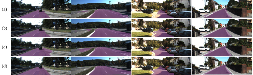
Figure 4: Example results on the KITTI benchmark: (a) MultiNet [2], (b) SNE-RoadSeg [7], (c) PLARD [6], and (d) Ours. Note that the outputs of these methods are probability maps of road, and we use 0.5 as the threshold to generate segmentation maps.

IV-D Loss Functions for Uncertainty Learning and Fusion

Given an image $I\in\mathbb{R}^{H\times W\times 3}$, we assign a one-hot label $\mathbf{y}\in\mathbb{R}^{H\times W\times 2}$, where $H,W$ denote height and width. Here, $\mathbf{y}_{i}\in\mathbb{R}^{2}$ is the labels of pixel $i$, $\mathbf{y}_{i,k}\in\{0,1\}$ is a binary value with $\mathbf{y}_{i,1}$ meaning the value of pixel $i$ in the road mask, and $\mathbf{y}_{i,0}$ for that in the non-road mask, where $i\in\{1,2...,HW\}$. $\bm{\alpha}=[\alpha_{0},\alpha_{1}]$ denotes the total concentration parameter of both road and non-road, and $\bm{\alpha}_{i}$ denotes pixel $i$ on $\bm{\alpha}$. The Dirichlet distribution can be formed as $D(\mathbf{p}_{i}|\bm{\alpha}_{i})$, where $\mathbf{p}_{i}$ is the class assignment probabilities of pixel $i$ on a simplex, and $\mathbf{p}_{i,k}$ is the pixel’s probability of class $k$. Referring to [28], the adjusted cross-entropy loss is used to guide USNet to generate more evidence for the correct prediction:

$$L_{a}(\!\bm{\alpha}_{i}\!)\!= \int\!\![\sum\nolimits_{k=0}^{1}\!-\mathbf{y}_{i,k}log(\!\mathbf{p}_{i,k}\!)\!]\!\frac{1}{B(\bm{\alpha}_{i})}\!\!\prod\nolimits_{k=0}^{1}\!(\!\mathbf{p}_{i,k}\!)^{\bm{\alpha}_{i,k}\!-\!1}d\mathbf{p}_{i}$$ (6)

$$\!= \sum\nolimits_{k=0}^{1}\mathbf{y}_{i,k}(\psi(S_{i})-\psi(\bm{\alpha}_{i,k}))$$

where $B(\cdot)$ is the beta function and $\psi(\cdot)$ is the digamma function. And the following Kullback-Leibler (KL) divergence [28] is used to limit the evidence for the negative label to $0$:

$$KL[D(\mathbf{p}_{i}\mid\tilde{\bm{\alpha}}_{i})\parallel D(\mathbf{p}_{i}\mid\mathbf{1})]=log(\frac{\Gamma({\sum_{k=0}^{1}}\tilde{\alpha}_{i,k})}{\Gamma(2){\prod_{k=0}^{1}}\Gamma(\tilde{\alpha}_{i,k})})+$$ (7)

$${\sum\nolimits_{k=0}^{1}}(\tilde{\alpha}_{i,k}-1)[\psi(\tilde{\alpha}_{i,k})-\psi({\sum\nolimits_{l=0}^{1}}\tilde{\alpha}_{i,l})]$$

where $\tilde{\bm{\alpha}}_{i}=\mathbf{y}_{i}+(\textbf{1}-\mathbf{y}_{i})\odot\bm{\alpha}_{i}$ is a filtered Dirichlet parameter, which is used to avoid the punishment to the positive label. $\Gamma(\cdot)$ is the gamma function. Then, the adjusted cross-entropy loss and this KL term are unified as follows:

$$L(\bm{\alpha}_{i})=L_{a}(\bm{\alpha}_{i})+\lambda_{t}KL[D(\mathbf{p}_{i}\mid\tilde{\bm{\alpha}}_{i})\parallel D(\mathbf{p}_{i}\mid\mathbf{1})]$$ (8)

where $\lambda_{t}=min(1,t/50)\in[0,1]$ is the balance factor, $t$ is the index of the current training epoch. We employ the unified loss to optimize the two subnetworks and the final prediction:

$$\mathcal{L}\!=\!\!\sum_{i=1}^{HW}\!\Big{(}\!\beta L(\bm{\alpha}_{i})\!+\!L(\bm{\alpha}_{i}^{\mathbf{r}})\!+\!L(\bm{\alpha}_{i}^{\mathbf{d}})\!+\!\sum_{h=1}^{3}\!\!\big{(}L([\bm{\alpha}_{i}^{\mathbf{r}}]^{h})\!+\!L([\bm{\alpha}_{i}^{\mathbf{d}}]^{h})\big{)}\!\!\Big{)}$$ (9)

where $\beta$ is a factor empirically set to $2$. $\bm{\alpha}^{\mathbf{r}}=[e_{0}^{\mathbf{r}}+1,e_{1}^{\mathbf{r}}+1]$ and $\bm{\alpha}^{\mathbf{d}}=[e_{0}^{\mathbf{d}}+1,e_{1}^{\mathbf{d}}+1]$ denote the parameters of the Dirichlet distribution of RGB and depth subnetworks, respectively. $h$ is the index of path of the MEC module. Our network is trained end-to-end based on the unified loss.

V EXPERIMENTS

In this section, we conduct comprehensive experiments to validate the performance of the proposed network.

V-A Experiment Setup

Datasets: Our experiments are carried out on the KITTI road dataset [17] and Cityscapes dataset [18]. The KITTI dataset is one of the most popular datasets for road segmentation. It contains 289 training images and 290 testing images. In the ablation study, we split the training set into two subsets: 253 samples for training and 36 samples for validating. The Cityscapes dataset is collected for urban scene semantic segmentation. It contains 2975 training images and 500 validating images annotated in 19 classes, while in our work, we only reserve the label for the road and re-label other classes as non-road.

Evaluation Metrics: For quantitative evaluation, we take the widely used pixel-wise segmentation metrics of road segmentation. The metrics include maximum F1-measure (MaxF), precision (PRE), recall (REC), false-positive rate (FPR) and false-negative rate (FNR). It is worth noting that the metrics are computed in the Birds Eye View (BEV) for the KITTI dataset as a common practice. We also evaluate the parameters, FLOPs, and inference time of our network.

Implementation Details: Our network is implemented using Pytorch and trained on a single NVIDIA GTX 1080Ti GPU. A ResNet-18 [32] model pre-trained on ImageNet [36] is employed as the backbone of USNet. In our experiment, the input images are resized to $384\times 1248$ for the KITTI dataset and $512\times 1024$ for the Cityscapes dataset. The loss is optimized by the AdamW [37] optimizer. We set the learning rate to $1e^{-4}$ for parameters of the backbone and $1e^{-3}$ for other parameters during training. For data augmentation, we use Gaussian blur, Gaussian noise, random horizontal flip, and random color jitter on the input images.

V-B Evaluation Results

In this subsection, the results on the KITTI dataset and the Cityscapes dataset are given.

KITTI Benchmark: We report the performance on the KITTI benchmark in Table I. Our method exhibits a MaxF of $96.89\%$, which outperforms all RGB-based methods and most RGB-LiDAR and RGB-D based methods. The boosting is mainly owing to the use of a more efficient uncertainty-aware RGB-D fusion strategy. Note that, the PLARD [6] that has a MaxF of $97.03\%$ is trained on multiple datasets, while our USNet is only trained on the KITTI dataset. Although the recent proposed SNE-RoadSeg+ [9] achieves a higher MaxF, it is 4$\times$ slower than our method (80 ms vs. 20 ms). Thus, our method achieves a better trade-off between the accuracy and model’s capacity. Moreover, the pixel-wise uncertainty given by USNet has great significance in guiding other self-driving modules, e.g., obstacle avoidance, path planning, etc., which is not available in existing methods.

Qualitative results are shown in Fig. 4. In detail, the first column visualizes a street where the boundary between road and sidewalk is unclear, MultiNet [2] and PLARD [6] suffer from the false positives, while USNet and SNE-RoadSeg [7] segment the road accurately with the assist of depth image. In the second column, other methods generate false segmentation in the left lane, but our method avoids this mis-classification. The third column shows a scene with over-exposure. Our method outperforms the other three methods in this situation, as depth data is used to compensate for the weakness of the RGB image in this scene effectively. The last scene has the same problem as the first column, and our method consistently generates precise segmentation. These results prove the effectiveness and reliability of our method.

Cityscapes Dataset: We also conduct experiments on the Cityscapes dataset. In the training process, we only reserve the label for road and treat other classes as non-road. The samples containing no road pixels are excluded from our evaluation. As shown in Table II, our method exceeds all other methods, especially outperforming RBANet [3] by $0.27\%$ MaxF, $0.39\%$ precision, and $0.15\%$ recall, which proves the generalization of our method.

TABLE II: Evaluation results on the Cityscapes validation set

Methods	MaxF(%)	PRE(%)	REC(%)
Zohourian et al. [38]	92.44	89.08	96.76
FCN [21]	94.68	93.69	95.70
s-FCN-loc [23]	95.36	94.63	96.11
SegNet [39]	95.81	94.55	97.11
RBANet [3]	98.00	97.87	98.13
Ours	98.27	98.26	98.28

V-C Ablation Studies

TABLE III: comparison with feature fusion models

Fusion settings	MaxF(%)	PRE(%)	REC(%)	FPR(%)	FNR(%)
Add	96.96	97.13	96.79	1.70	3.21
Cat+Conv	96.97	96.91	97.03	1.84	2.97
RFNet [40]	97.04	96.67	97.41	2.00	2.59
ACNet [41]	97.02	96.76	97.28	1.94	2.72
SA-Gate [42]	97.12	96.67	97.58	2.00	2.42
Ours	97.31	97.20	97.42	1.67	2.58

TABLE IV: Effectiveness analysis of proposed modules.

Settings	MaxF(%)	PRE(%)	REC(%)	FPR(%)	FNR(%)
RGB	95.28	94.44	96.12	3.37	3.88
Depth	96.64	96.14	97.15	2.32	2.85
RGB-D	97.01	96.65	97.38	2.01	2.62
RGB-D+MEC	97.16	96.99	97.33	1.80	2.67
RGB-D+UAF	97.19	97.04	97.34	1.76	2.66
Ours	97.31	97.20	97.42	1.67	2.58

TABLE V: Comparison of efficiency on the KITTI dataset

Methods	Params(M)	FLOPs(G)	FPS	MaxF(%)
MultiNet [2]	134.3	406.5	11.6	94.88
SNE-RoadSeg [7]	201.3	1950.2	4.5	96.75
PLARD [6]	76.9	1147.6	4.3	96.83
Ours	30.7	78.2	43.6	96.89

This section gives considerable experiments to thoroughly analyze our network on the KITTI dataset.

Comparison with Feature Fusion Models: To verify the superiority of our fusion paradigm compared to previous works [7, 8, 24, 9], we test several feature fusion strategies by five variants. Each variant contains two encoders and one decoder, and the feature maps of corresponding layers in the two encoders are fused in different ways. As shown in Table III, the ‘Add’ indicates directly summing the feature of RGB and depth, and ‘Cat+Conv’ indicates fusing by concatenation and convolution. ‘RFNet’, ‘ACNet’ and ‘SA-Gate’ indicate using the fusion strategy proposed in the semantic segmentation networks [40, 41, 42], respectively. Our USNet achieves the best MaxF than those models using other fusion strategies. The comparison indicates that the different characteristics of the RGB and depth are not well perceived by directly fusing the features of the two modalities.

Effectiveness of Proposed Modules: We verify the effectiveness of each component in the proposed network, including two subnetworks, the multi-scale evidence collection (MEC) module, and the uncertainty-aware fusion (UAF) module. First, to evaluate the necessity of the two subnetworks, we conduct experiments based on only one modality. As shown in Table IV, the RGB-based model and depth-based model achieve $95.28\%$ and $96.64\%$ in terms of MaxF, while RGB-D based model improves the MaxF to $97.01\%$, Note that, in the RGB-D based model, we fuse the segmentation result of the two subnetworks by simple addition. Furthermore, when MEC and UAF modules are utilized separately, the MaxF increases by $0.15\%$ and $0.18\%$ respectively, proving the effectiveness of MEC and UAF. Finally, when all these components are used, we obtain the best MaxF of $97.31\%$. The reason is that the MEC provides more evidence to UAF for more sufficient determination.

V-D Efficiency Analysis

We analyze the computational efficiency of the proposed method in comparison with three open-source methods. All speeds are gained on a same computer equipped with an NVIDIA GTX 1080Ti GPU, and the input images are scaled into $384\times 1248$ resolution for a fair comparison. As observed in Table V, the parameters and FLOPs of our network is much fewer than other methods, which is owing to the simplified backbone and zero-parameter decoder. Meanwhile, our network can run at 43.6 FPS, 4$\times$ faster than MultiNet [2], and 10$\times$ faster than PLARD [6] and SNE-RoadSeg [7]. In particular, compared to SNE-RoadSeg [7], i.e., an RGB-D based method, USNet reduces the parameter by $85\%$, and the FLOPs by $96\%$, but gains $0.14\%$ improvement on MaxF (see Table I). Thus, the USNet is more suitable for real-time applications intuitively and has the potential to further boost the speed to reach the requirement of embedded platforms.

VI Conclusion

In this work, we propose a novel low-latency RGB-D road segmentation network named USNet, which adopts a light-weight symmetric network to separately perceive road representations based on RGB and depth data. For collecting more valuable evidence from each subnetwork, an MEC is proposed. Besides, a UAF module is designed to obtain the uncertainty of the two modalities and generate the final segmentation. All these effective designs enable our model to work satisfyingly in terms of both accuracy and computational cost.

References

- [1] G. L. Oliveira, W. Burgard, and T. Brox, “Efficient deep models for monocular road segmentation,” in IEEE/RSJ International Conference on Intelligent Robots and Systems (IROS), 2016.
- [2] M. Teichmann, M. Weber, M. Zöllner, R. Cipolla, and R. Urtasun, “Multinet: Real-time joint semantic reasoning for autonomous driving,” in IEEE Intelligent Vehicles Symposium (IV), 2018.
- [3] J. Y. Sun, S. W. Kim, S. W. Lee, Y. W. Kim, and S. J. Ko, “Reverse and boundary attention network for road segmentation,” in IEEE/CVF International Conference on Computer Vision Workshop (ICCVW), 2019.
- [4] L. Caltagirone, M. Bellone, L. Svensson, and M. Wahde, “Lidar-camera fusion for road detection using fully convolutional neural networks,” Robotics and Autonomous Systems (RAS), vol. 111, pp. 125–131, 2019.
- [5] S. Gu, J. Yang, and H. Kong, “A cascaded lidar-camera fusion network for road detection,” in IEEE International Conference on Robotics and Automation (ICRA), 2021.
- [6] Z. Chen, J. Zhang, and D. Tao, “Progressive lidar adaptation for road detection,” IEEE/CAA Journal of Automatica Sinica (JAS), vol. 006, no. 003, pp. P.693–702, 2019.
- [7] R. Fan, H. Wang, P. Cai, and M. Liu, “SNE-RoadSeg: Incorporating surface normal information into semantic segmentation for accurate freespace detection,” in European Conference on Computer Vision (ECCV), 2020.
- [8] H. Wang, R. Fan, Y. Sun, and M. Liu, “Applying surface normal information in drivable area and road anomaly detection for ground mobile robots,” in IEEE/RSJ International Conference on Intelligent Robots and Systems (IROS), 2020.
- [9] H. Wang, R. Fan, P. Cai, and M. Liu, “SNE-RoadSeg+: Rethinking depth-normal translation and deep supervision for freespace detection,” in IEEE/RSJ International Conference on Intelligent Robots and Systems (IROS), 2021.
- [10] Y. Gao, X. Li, J. Zhang, Y. Zhou, D. Jin, J. Wang, S. Zhu, and X. Bai, “Video text tracking with a spatio-temporal complementary model,” IEEE Transactions on Image Processing (TIP), vol. 30, pp. 9321–9331, 2021.
- [11] Y. Zhou, X. Bai, W. Liu, and L. J. Latecki., “Similarity fusion for visual tracking,” International Journal of Computer Vision (IJCV), vol. 118, no. 3, pp. 337–363, 2016.
- [12] Y. Zhou, X. Bai, W. Liu, and L. Latecki, “Fusion with diffusion for robust visual tracking,” in Advances in Neural Information Processing Systems (NIPS), 2012.
- [13] J. Ma, A. Ming, Z. Huang, X. Wang, and Y. Zhou, “Object-level proposals,” in IEEE International Conference on Computer Vision (ICCV), 2017.
- [14] M. Zhou, J. Ma, A. Ming, and Y. Zhou, “Objectness-aware tracking via double-layer model,” in IEEE International Conference on Image Processing (ICIP), 2018.
- [15] F. Xue, A. Ming, M. Zhou, and Y. Zhou, “A novel multi-layer framework for tiny obstacle discovery,” in International Conference on Robotics and Automation (ICRA), 2019.
- [16] F. Xue, A. Ming, and Y. Zhou, “Tiny obstacle discovery by occlusion-aware multilayer regression,” IEEE Transactions on Image Processing (TIP), vol. 29, pp. 9373–9386, 2020.
- [17] J. Fritsch, T. Kühnl, and A. Geiger, “A new performance measure and evaluation benchmark for road detection algorithms,” in International IEEE Conference on Intelligent Transportation Systems (ITSC), 2013.
- [18] M. Cordts, M. Omran, S. Ramos, T. Rehfeld, M. Enzweiler, R. Benenson, U. Franke, S. Roth, and B. Schiele, “The cityscapes dataset for semantic urban scene understanding,” in IEEE Conference on Computer Vision and Pattern Recognition (CVPR), 2016.
- [19] R. Chandra, U. Bhattacharya, T. Randhavane, A. Bera, and D. Manocha, “Roadtrack: Realtime tracking of road agents in dense and heterogeneous environments,” in IEEE International Conference on Robotics and Automation (ICRA), 2020.
- [20] Y. Zhou., Y. Yang., Y. Meng., X. Bai, W. Liu, and L. J. Latecki., “Online multiple person detection and tracking from mobile robot in cluttered indoor environments with depth camera,” International Journal of Pattern Recognition and Artificial Intelligence (IJPRAI), vol. 28, no. 1, pp. 1 455 001.1–1 455 001.28, 2014.
- [21] J. Long, E. Shelhamer, and T. Darrell, “Fully convolutional networks for semantic segmentation,” in IEEE Conference on Computer Vision and Pattern Recognition (CVPR), 2015.
- [22] C. Zhe and Z. Chen, “Rbnet: A deep neural network for unified road and road boundary detection,” in International Conference on Neural Information Processing (ICONIP), 2017.
- [23] J. Gao, Q. Wang, and Y. Yuan, “Embedding structured contour and location prior in siamesed fully convolutional networks for road detection,” in IEEE International Conference on Robotics and Automation (ICRA), 2017.
- [24] H. Wang, R. Fan, Y. Sun, and M. Liu, “Dynamic fusion module evolves drivable area and road anomaly detection: A benchmark and algorithms,” IEEE Transactions on Cybernetics (TCYB), pp. 1–11, 2021.
- [25] S. Xie and Z. Tu, “Holistically-nested edge detection,” in IEEE International Conference on Computer Vision (ICCV), 2015.
- [26] S. Ren, K. He, R. Girshick, and J. Sun, “Faster r-cnn: Towards real-time object detection with region proposal networks,” IEEE Transactions on Pattern Analysis and Machine Intelligence (TPAMI), vol. 39, no. 6, pp. 1137–1149, 2017.
- [27] Z. Liu, X. Zhao, T. Huang, R. Hu, Y. Zhou, and X. Bai, “TANet: Robust 3d object detection from point clouds with triple attention,” in AAAI Conference on Artificial Intelligence(AAAI), 2020.
- [28] M. Sensoy, L. M. Kaplan, and M. Kandemir, “Evidential deep learning to quantify classification uncertainty,” in Neural Information Processing Systems (NIPS), 2018.
- [29] Z. Han, C. Zhang, H. Fu, and J. T. Zhou, “Trusted multi-view classification,” in International Conference on Learning Representations (ICLR), 2021.
- [30] A. P. Dempster, “A generalization of bayesian inference,” Journal of the Royal Statistical Society: Series B (Methodological), vol. 30, no. 2, pp. 205–232, 1968.
- [31] A. JSANG, Subjective Logic: A formalism for reasoning under uncertainty. Springer, 2018.
- [32] K. He, X. Zhang, S. Ren, and J. Sun, “Deep residual learning for image recognition,” in IEEE Conference on Computer Vision and Pattern Recognition (CVPR), 2016.
- [33] R. Lu, F. Xue, M. Zhou, A. Ming, and Y. Zhou, “Occlusion-shared and feature-separated network for occlusion relationship reasoning,” in IEEE/CVF International Conference on Computer Vision (ICCV), 2019.
- [34] L.-C. Chen, G. Papandreou, I. Kokkinos, K. Murphy, and A. L. Yuille, “Deeplab: Semantic image segmentation with deep convolutional nets, atrous convolution, and fully connected crfs,” IEEE Transactions on Pattern Analysis and Machine Intelligence (TPAMI), vol. 40, no. 4, pp. 834–848, 2018.
- [35] J. Hu, L. Shen, S. Albanie, G. Sun, and E. Wu, “Squeeze-and-excitation networks,” IEEE Transactions on Pattern Analysis and Machine Intelligence (TPAMI), vol. 42, no. 8, pp. 2011–2023, 2020.
- [36] J. Deng, W. Dong, R. Socher, L.-J. Li, K. Li, and L. Fei-Fei, “Imagenet: A large-scale hierarchical image database,” in IEEE Conference on Computer Vision and Pattern Recognition (CVPR), 2009.
- [37] D. P. Kingma and J. Ba, “Adam: A method for stochastic optimization,” in International Conference on Learning Representations (ICLR), 2015.
- [38] F. Zohourian, B. Antic, J. Siegemund, M. Meuter, and J. Pauli, “Superpixel-based road segmentation for real-time systems using cnn.” in International Joint Conference on Computer Vision, Imaging and Computer Graphics Theory and Applications (VISIGRAPP), 2018.
- [39] V. Badrinarayanan, A. Kendall, and R. Cipolla, “Segnet: A deep convolutional encoder-decoder architecture for image segmentation,” IEEE Transactions on Pattern Analysis and Machine Intelligence (TPAMI), vol. 39, no. 12, pp. 2481–2495, 2017.
- [40] L. Sun, K. Yang, X. Hu, W. Hu, and K. Wang, “Real-time fusion network for rgb-d semantic segmentation incorporating unexpected obstacle detection for road-driving images,” IEEE Robotics and Automation Letters (RA-L), vol. 5, no. 4, pp. 5558–5565, 2020.
- [41] X. Hu, K. Yang, L. Fei, and K. Wang, “Acnet: Attention based network to exploit complementary features for rgbd semantic segmentation,” in IEEE International Conference on Image Processing (ICIP), 2019.
- [42] X. Chen, K.-Y. Lin, J. Wang, W. Wu, C. Qian, H. Li, and G. Zeng, “Bi-directional cross-modality feature propagation with separation-and-aggregation gate for rgb-d semantic segmentation,” in European Conference on Computer Vision (ECCV), 2020.