Riemann problem of Euler equations with singular sources

Abstract

This paper is concerned with the Riemann problem of one-dimensional Euler equations with a singular source. The exact solution of this Riemann problem contains a stationary discontinuity induced by the singular source, which is different from all the simple waves in the Riemann solution of classical Euler equations. We propose an eigenvalue-based monotonicity criterion to select the physical curve of this stationary discontinuity. By including this stationary discontinuity as an elementary wave, the structure of Riemann solution becomes diverse, e.g. the number of waves is not fixed and interactions between two waves become possible. Under the double CRP framework, we prove all possible structures of the Riemann solution.

Keywords: hyperbolic conservation law, Euler equation, Riemann problem, singular source, entropy condition

AMS subject classifications: 35L67,35Q31,76N30

1 Introduction

In governing equations for fluids, the effects other than convection and diffusion are usually described by source terms. Sources can exhibit singularities in some complex problems, such as surface tension [16, 24], evaporation[10, 11, 12], phase transition[22, 31, 36, 39], condensation[8], geometric constraints[9, 33, 35]. The singular source induces jumps in the state of flow and leads to new difficulties in the analysis of fluid motion.

This paper focuses on investigating the effect of singular sources on flow field for inviscid compressible fluids. The governing equations are

$$\partial_{t}U+\partial_{x}F(U)=\delta(x)S,$$ (1.1)

where

$$U=\begin{pmatrix}\rho\\ \rho u\\ E\end{pmatrix},F=\begin{pmatrix}\rho u\\ \rho u^{2}+p\\ (E+p)u\end{pmatrix},\delta(x)=\begin{cases}0,\ x\neq 0\\ \infty,\ x=0\end{cases}$$

Here, $\rho$, $p$ and $E$ denote the density, pressure and total energy, respectively. $u$ is the velocity. $S$ is the vector of souce term. $\delta(x)$ is the Dirac delta function, which means that the source term is only distributed at the origin.

Some existing studies on hyperbolic conservation laws with singular sources assume that the singular source depends continuously on the local state of the flow field, such as [41, 21, 10, 44, 25]. Since the states of the flow fields on either side of the singular source are generally discontinuous, we focus on a more general model in which the source depends explicitly on the states on either side in the present work. A typical example is the model of condensation of wet gas in a nozzle, where the rate of condensation is determined only by the state of upstream flow (see [40, 14, 8]).

For simplicity, we assume that the value of $S$ is proportional to the flux upstream of the origin.

$$S(U_{-},U_{+})=\begin{cases}S(F(U_{-}))=diag(k_{1},k_{2},k_{3})F(U_{-}),\ \text{if}\ u_{-}>0,u_{+}>0\\ S(F(U_{+}))=diag(k_{1},k_{2},k_{3})F(U_{+}),\ \text{if}\ u_{-}<0,u_{+}<0\\ 0,\ else\\ \end{cases}$$ (1.2)

where

$$U_{-}=U(0-,t),\ U_{+}=U(0+,t),$$

$diag(k_{1},k_{2},k_{3})$ is the diagonal matrix with constant diagonal element $k_{1}$, $k_{2}$ and $k_{3}$. The models in [14] can be considered as a special case of the above model.

A basic assumption is that the fluid cannot lose more mass, momentum and energy than the corresponding total amount flowing into the origin, which implies

$$k_{1}>-1,k_{2}>-1,k_{3}>-1.$$

When the fluid at the origin is in equilibrium, the upstream and downstream velocities have the same sign. For the non-equilibrium state where these two velocities have different signs, we set the value of source to zero. We assume that the fluid is polytropic ideal and thermally ideal, whose equation of state is given by

$$RT=p/\rho,\ p=(\gamma-1)\rho e,\ \gamma>1,$$

where $\gamma$ is the ratio of specific heats, $e$ is the internal energy, $T$ is the temperature and $R$ is the universal gas constant. The Riemann problem of (1.1) is a Cauchy problem with piecewise constant initial values

$$\begin{cases}\partial_{t}U+\partial_{x}F(U)=\delta(x)S\\ U(x,0)=\begin{cases}U_{L},\ x<0\\ U_{R},\ x>0\end{cases}\end{cases}$$ (1.3)

A typical feature of the Riemann solution of hyperbolic conservation law with singular sources is that it contains a new kind of wave, which appears as a stationary discontinuity. Without a restriction on this new discontinuity, the Riemann solution is not unique(see [20, 21]), thus we need to first set up an admissibility condition to select the physical solution. It is very difficult to establish an admissibility condition from the global solution, and very limited work has been done, such as a minimum principle proposed by J.M.Greenberg et al.[20] by a prior estimation. A simpler and more practical approach is to limit the state on both sides of this new discontinuity, that is, to restrict the steady solution near the stationary discontinuity rather than the global Riemann solution, as in the Lax shock inequality(see [28, 29]). The admissibility condition established in this way has been successfully applied to the shallow water equations(see [33, 34]), the equations of flows in a nozzle(see [26, 27, 32, 41]) and the equations of flow with heat addition(see [4, 8, 13, 14, 40]). We find that those admissibility condition for different equations are equivalent in the representation of eigenvalues, which motivates us to propose an eigenvalue-based condition in this work. We apply the present proposed condition to (1.1) and study the wave curve for the new disontinuity. Following the nomenclature in [26, 27, 32, 33, 34, 41, 42], the present proposed condition is still named as a monotonicity criterion, since it also leads to a kind of monotonicity of the new discontinuity.

In general, the singular source causes the structure of Riemann solution to become complicated. For example, the number of waves is not fixed, and the waves may interact with each other(see [3, 5, 8, 33, 34, 38, 41, 45, 46]). A common way to analyze such a kind of Riemann problem is to convert the original non-homogeneous system into a homogeneous system by adding an augmented equation, and the discontinuity induced by the singular sources can then be associated with a new linearly degenerate characteristic domain of augmented equations. There are a number of representative works that analyse Riemann problem by the augmented equations, and we refer readers to [5, 15, 17, 33, 38, 41] for details. In form, we can also convert the Riemann problem (1.3) into the Riemann problem of a homogeneous system:

$$\begin{cases}\partial_{t}\begin{pmatrix}U\\ h\end{pmatrix}+\partial_{x}\begin{pmatrix}F(U)\\ 0\end{pmatrix}-\begin{pmatrix}S\partial_{x}h\\ 0\end{pmatrix}=0,\\ U(x,0)=\begin{cases}U_{L},\ x<0\\ U_{R},\ x>0\end{cases}\ h(x,0)=\begin{cases}0,\ x<0\\ 1,\ x>0\end{cases}\end{cases}$$ (1.4)

The augmented system is nonconservative equations, and the term $S\partial_{x}h$ is the product of two distributions at the origin. The theory of nonconservative product has been developed to give a clear definition of this type of product, see [2, 6, 18, 19, 21, 30, 37, 23]. However, we would not use (1.4) to obtain the Riemann solution in this paper. The reason being that the discontinuity of $S$, which is different from other common singular sources, forces us to redesign reasonable non-conservative paths. In addition, Abgrall, Bacigaluppi and Tokareva (2018) commented that ”A nonconservative formulation of the system and getting the correct solution has been a long-standing debate”(p.10)[1].

In this paper we obtain the exact solution to Riemann problem (1.3) by a double classical Riemann problem(CRP) framework[45, 46]. In the x-t plane, the singular source is constantly located at the t-axis, so that the Riemann solutions in the left and right half-planes of the origin satisfy the classical Euler equations. Under the double CRP framework, the solution of CRP in the left half-plane, the steady solution near the singular source and the solution of CRP in the right half-plane are discussed separately and then coupled to obtain the Riemann solution in the full plane.

This paper is organized as follows. In Section2 we will present all the elementary waves of Riemann solution, including the three simple waves associated with the classical Euler equations and a new kind of discontinuity induced by singular sources. We will give the wave curve of that new discontinuity under the monotonicity criterion. Section3 contains the proof of all possible structures of Riemann solution. Finally, some conclusions will be given in Section4.

2 Elementary waves

In this section we present elementary waves in self-similar solutions of Riemann problem (1.3), including a new discontinuity induced by the singular source term, called the stationary wave, and elementary waves in the Riemann solutions of classical Euler equations.

2.1 Stationary wave

The singular source term causes the state of flow to jump when it passes through the origin. This discontinuity is called the stationary wave and is regarded as a new elementary wave of the Riemann solution. Its left-hand state $U_{-}$ and right-hand state $U_{+}$ satisfy the jump relation:

$$F(U_{-})+S(F(U_{-}))=F(U_{+}),$$ (2.1)

and the component-wise form is

$$\begin{cases}\rho_{-}u_{-}(1+k_{1})=\rho_{+}u_{+},\\ (\rho_{-}u_{-}^{2}+p_{-})(1+k_{2})=\rho_{+}u_{+}^{2}+p_{+},\\ (E_{-}+p_{-})u_{-}(1+k_{3})=(E_{+}+p_{+})u_{+}.\end{cases}$$ (2.2)

If the left-hand state $U_{-}$ and right-hand state $U_{+}$ of $U$ at the origin satisfy (2.1), then $U$ is a steady solution of (1.1) near the origin. $U_{-}$ and $U_{+}$ are called equilibrium states. By the first eqution of (2.2), we know that $u_{-}$ and $u_{+}$ have the same sign. One of the values of $u_{-}$ and $u_{+}$ being zero results in the other also being zero, which causes the source term to vanish and the governing equation (1.1) to degenerate to the classical Euler equations. Hence we will only consider the case of $u_{-}>0,u_{+}>0$, as the case of $u_{-}<0,u_{+}<0$ can be changed to that by a transformation $x\mapsto-x,u\mapsto-u$.

When $S=0(k_{1}=k_{2}=k_{3}=0)$, there are two $U_{+}$ that satisfy (2.1) for a given $U_{-}$, and the Mach numbers of $U_{+}$ are

$$M_{+}=M_{-}\ \text{or}\ \sqrt{\frac{(\gamma-1)M_{-}^{2}+2}{2\gamma M_{-}^{2}+1-\gamma}}.$$

When $S\neq 0$, we can obtain an explicit expression of $U_{+}$ by a tedious computation similar to that used in [45, 4, 8]. There are also two solutions of $U_{+}$, and their Mach numbers are denoted by

$$M_{+}^{(1)}=\sqrt{\frac{1-I}{1+\gamma I}},\quad M_{+}^{(2)}=\sqrt{\frac{1+I}{1-\gamma I}},$$ (2.3)

where

$$I=I(M_{-})=\frac{\sqrt{(\gamma M_{-}^{2}+1)^{2}-(\gamma+1)M_{-}^{2}[(\gamma-1)M_{-}^{2}+2](1+k_{1})(1+k_{3})/(1+k_{2})^{2}}}{\gamma M_{-}^{2}+1}.$$

$M_{+}^{(1)}$ is well-defined iff

$$(\gamma M_{-}^{2}+1)^{2}\geq(\gamma+1)M_{-}^{2}[(\gamma-1)M_{-}^{2}+2](1+k_{1})(1+k_{3})/(1+k_{2})^{2}.$$ (2.4)

$M_{+}^{(2)}$ is well-defined iff

$$\text{equation}(\ref{equ: Mach number condition1})\ \&\ \gamma I\leq 1.$$ (2.5)

Since $I$ is not less than zero, we have

$$M_{+}^{(1)}\leq 1,\ M_{+}^{(2)}\geq 1.$$ (2.6)

$M_{+}^{(1)}$ and $M_{+}^{(2)}$ are referred to as the subsonic and supersonic branches, respectively. Besides, a standard computation(see [4]) gives rise to

$$\frac{\rho_{+}}{\rho_{-}}=\left(\frac{M_{-}}{M_{+}}\right)^{2}\frac{\gamma M_{+}^{2}+1}{\gamma M_{-}^{2}+1}\frac{(1+k_{1})^{2}}{1+k_{2}},$$

$$\frac{u_{+}}{u_{-}}=\left(\frac{M_{+}}{M_{-}}\right)^{2}\frac{\gamma M_{-}^{2}+1}{\gamma M_{+}^{2}+1}\frac{1+k_{2}}{1+k_{1}},$$

$$\frac{p_{+}}{p_{-}}=\frac{\gamma M_{-}^{2}+1}{\gamma M_{+}^{2}+1}(1+k_{2}).$$

That is, the ratio of other states between downstream and upstream can be determined by the Mach numbers $M_{-}$ and $M_{+}$. With $M_{-}\in(0,\infty)$ as an independent variable, $M_{+}^{(1)}$ and $M_{+}^{(2)}$ defined by (2.3) can be regarded as functions of $M_{-}$, then it can be proved that

Property 2.1

Under (2.4), $M_{+}^{(1)}(M_{-})$ is increasing when $M_{-}\in(0,1]$ and decreasing when $M_{-}\in[1,\infty)$. Under (2.5), $M_{+}^{(2)}(M_{-})$ is decreasing when $M_{-}\in(0,1]$ and increasing when $M_{-}\in[1,\infty)$.

The quasilinear form of the inhomogeneous Euler equations (1.1) is

$$\partial_{t}U+A(U)\partial_{x}U=\delta(x)S,$$

where $A(U)=\partial F/\partial U$. This equation is strictly hyperbolic, and the eigenvalues of $A(U)$ are

$$\lambda_{1}=u-a<\lambda_{2}=u<\lambda_{3}=u+a,$$

where $a$ is the speed of sound.

The two solutions (2.3) of $M_{+}$ may be nonphysical, therefore an admissibility condition called monotonicity criterion is given below to select the physical solution of (2.1).

Monotonicity Criterion 1

Given coefficients $k_{1}$, $k_{2}$ and $k_{3}$, the left-hand state $U_{-}$ and right-hand state $U_{+}$ of a statiaonry wave satisfies $\lambda_{k}(U_{-})\cdot\lambda_{k}(U_{+})\geq 0,\forall 1\leq k\leq 3$.

Criterion1 restricts each corresponding eigenvalue of the left-hand and right-hand states of stationary wave from having opposite signs. When a certain eigenvalue of the state on one side is zero, Criterion1 loses its restriction on the corresponding eigenvalue of the state on the other side. Following the definition of thermal choke in [14, 13, 8, 4], we define this particular state as choke as well.

Definition 2.1

A stationary wave is said to be choked if its left-hand state $U_{-}$ and right-hand state $U_{+}$ satisfy $\exists 1\leq k\leq m,s.t.\ \lambda_{k}(U_{-})\cdot\lambda_{k}(U_{+})=0$.

A Riemann solution is said to be choked if it contains a choked stationary wave.

Remark 2.1

Criterion1 can be applied to Generalized hyperbolic conservation laws with singular source terms:

$$\partial_{t}U+\partial_{x}F(U)=\delta(x)S,$$ (2.7)

where $U$, $F$ and $S$ are all vector-valued functions of m components. If the self-similar solution to the Riemann problem of (2.7) contains a stationary wave on the t-axis with the left-hand state $U_{-}$ and the right-hand state $U_{+}$, then it satisfies $\lambda_{k}(U_{-})\cdot\lambda_{k}(U_{+})\geq 0,\forall 1\leq k\leq m$, where $\lambda_{k}(1\leq k\leq m)$ is the kth eigenvalue of the $m\times m$ matrix $\partial F/\partial U$.

Remark 2.2

Greenberg, Leroux, Baraille and Noussair[20] studied the Riemann problem of the scalar equation with a singular source term

$$\begin{cases}\partial_{t}U+\partial_{x}F(U)=c\delta(x),\\ U(x,0)=\begin{cases}U_{L},\ x<0\\ U_{R},\ x>0\end{cases}\end{cases}$$ (2.8)

where $U(x,t),F(U)$ are both scalar-valued functions, $F(0)=0,F^{\prime\prime}>0$, and $c$ is a constant coefficient. Greenberg et al. proposed a minimum principle, which is based on a priori estimate of the integral equation, to select the physical Riemann solutions. The expression of Criterion1 applied to (2.8) is $U_{-}\cdot U_{+}\geq 0$, by which we can obtain the values of $U_{-}$ and $U_{+}$ of Riemann solution. It’s easy to verify that the Riemann solutions based on Greenberg’s principle and the Riemann solutions based on the present Monotonicity Criterion are exactly the same in all cases.

Remark 2.3

The shallow water equations with discontinuous topography is a widely studied hyperbolic conservation law with singular source terms, and its Riemann problem is

$$\begin{cases}\frac{\partial h}{\partial t}+\frac{\partial hu}{\partial x}=0,\\ \frac{\partial hu}{\partial t}+\frac{\partial(h(u^{2}+gh/2))}{\partial x}=-gh\frac{\partial a}{\partial x},\\ (h,u,a)(x,0)=\begin{cases}(h_{L},u_{L},a_{L}),\quad x<0\\ (h_{R},u_{R},a_{R}),\quad x>0\end{cases}\end{cases}$$

Here, $h$ denotes the height of the water from the bottom to the surface, $u$ the velocity of the fluid, $g$ the gravity constant, and $a$ the height of the river bottom from a given level. The source term of shallow water equations differs from (1.1) in that it is continuously dependent on the conservative variable, therefore additional approximations are required to give a jump relation. The jump relation used in [34, 33, 3] is

$$\begin{cases}h_{-}u_{-}=h_{+}u_{+},\\ h_{-}+\frac{u_{-}^{2}}{2g}+a_{L}=h_{+}+\frac{u_{+}^{2}}{2g}+a_{R},\end{cases}$$

The subscripts ”_” and ”+” still denote the left-hand and right-hand states of t-axis of Riemann solution. The expression for Criterion1 applied to the shallow water equations is $F_{-}\cdot F_{+}\geq 0$, where $F$ is Froude number, which can be proved to be equivalent to the admissible principles used in previous literature(see [34, 33, 42]).

Remark 2.4

The jump relation (2.1) with $k_{1}=k_{2}=0,k_{3}>0$ is called equilibrium equation of heat addition problem(see [40, 14, 13]). The Euler equations with this particular source term has been used to study the condensation-induced waves in a slender Laval nozzle in [8]. The physical properties force the change of the state during heating not to cross the maximum entropy point in the Rayleigh line (see [4]), which equates to the Criterion1.

We call $U_{+}$ the solution to a stationary wave if $U_{+}$ satisfies (2.1) and Criterion1 for given $U_{-}$ and coefficients $k_{1},k_{2},k_{3}$. According to Criterion1 and (2.6), we can select the physical solutions between the two branches $M_{+}^{(1)}$ and $M_{+}^{(2)}$:

$$M_{+}=\begin{cases}M_{+}^{(1)}=\sqrt{\frac{1-I}{1+\gamma I}},\ \text{if}\ M_{-}\leq 1\\ M_{+}^{(2)}=\sqrt{\frac{1+I}{1-\gamma I}},\ \text{if}\ M_{-}\geq 1\end{cases}$$ (2.9)

According to (2.9), (2.4) and (2.5), the range of $M_{-}$ that ensures the existence of the physical solutions is

$$\Gamma_{-,k_{1},k_{2},k_{3}}\mathop{=}\limits^{def}\left((0,1]\cup\left([1,+\infty)\cap\left\{M_{-}|\gamma I(M_{-})\leq 1\right\}\right)\right)\cap$$

$$\left\{M_{-}|(\gamma M_{-}^{2}+1)^{2}\geq(\gamma+1)M_{-}^{2}[(\gamma-1)M_{-}^{2}+2](1+k_{1})(1+k_{3})/(1+k_{2})^{2}\right\},$$

which will be written simply as $\Gamma_{-}$ when no confusion can arise. We can now give a clear definition of the stationary wave.

Proposition 2.1 (Stationary wave curves)

Given a left-hand state $U_{-}$ with $u_{-}>0$, the stationary wave curve $\mathcal{D}(U_{-},k_{1},k_{2},k_{3})$ consisting of all right-hand states $U_{+}$ that can be connected to $U_{-}$ by a stationary wave with given coefficients $k_{1},k_{2},k_{3}$ under Criterion1, is

$$\mathcal{D}(U_{-},k_{1},k_{2},k_{3}): M_{+}=\begin{cases}M_{+}^{(1)}=\sqrt{\frac{1-I}{1+\gamma I}},\ M_{-}\in\Gamma_{-}\cap(0,1]\\ M_{+}^{(2)}=\sqrt{\frac{1+I}{1-\gamma I}},\ M_{-}\in\Gamma_{-}\cap[1,+\infty)\end{cases}$$

$$\rho_{+}=\rho_{-}\left(\frac{M_{-}}{M_{+}}\right)^{2}\frac{\gamma M_{+}^{2}+1}{\gamma M_{-}^{2}+1}\frac{(1+k_{1})^{2}}{1+k_{2}},$$

$$u_{+}=u_{-}\left(\frac{M_{+}}{M_{-}}\right)^{2}\frac{\gamma M_{-}^{2}+1}{\gamma M_{+}^{2}+1}\frac{1+k_{2}}{1+k_{1}},$$

$$p_{+}=p_{-}\frac{\gamma M_{-}^{2}+1}{\gamma M_{+}^{2}+1}(1+k_{2}).$$

Note 2.1

Although we refer to the set $\mathcal{D}(U_{-},k_{1},k_{2},k_{3})$ of solutions as a wave curve, it is not a one-parameter family. If the coefficients $k_{1},k_{2},k_{3}$ are taken as parameters, it is actually a three-parameter family. For given parameters $k_{1},k_{2},k_{3}$, each left-hand state $U_{-}$ determines its corresponding right state $U_{+}$, and we therefore say that the stationary wave has no degrees of freedom.

Property 2.2

The $M_{+}$ defined by (2.9) is a monotone increasing function of $M_{-}\in\Gamma_{-}\cap(0,1]$ and $M_{-}\in\Gamma_{-}\cap[1,+\infty)$.

It is clear from PropertyProperty2.1 that both branches $M_{+}^{(1)},M_{+}^{(2)}$ as a function of $M_{-}$ have a unique extreme value at $M_{-}=1$, and PropertyProperty2.2 shows that the Criterion1 works by choosing a branch such that the Mach number $M_{+}$ of physical solution is a piecewise monotonic function of $M_{-}$.

The solution of a stationary wave depends on the solution of Mach number $M_{+}$, as each $M_{+}$ corresponds to a unique state $U_{+}$. Similarly, we denote by $\Gamma_{+,k_{1},k_{2},k_{3}}$ the set of $M_{+}$, which is also written as $\Gamma_{+}$ when no confusion can arise. As will be seen in the next section, $\Gamma_{-}$ and $\Gamma+$ significantly affect the structure of the Riemann solution, therefore we give more explicit expressions for $\Gamma_{-}$ and $\Gamma_{+}$ below.

With the specific eigenvalues of Euler equations, an equivalent expression for Criterion1 as applied to one-dimensional Euler equations is

Monotonicity Criterion 2

Given coefficients $k_{1}$, $k_{2}$ and $k_{3}$, the left-hand state $U_{-}$ and right-hand state $U_{+}$ of a stationary wave satisfies $u_{-}\cdot u_{+}\geq 0$ and $(M_{-}-1)\cdot(M_{+}-1)\geq 0$.

The admissible region of Criterion2 in $M_{-}-M_{+}$ plane is $(0,1]\times(0,1]\cup[1,+\infty)\times[1,+\infty)$, as shown in the gray area in Figure1. We divide this area into four sub-areas as follows.

$$\Omega_{1}=\left\{(M_{-},M_{+})|0<M_{-}\leq 1,0<M_{+}\leq 1,M_{+}>M_{-}\right\}$$

$$\Omega_{2}=\left\{(M_{-},M_{+})|0<M_{-}\leq 1,0<M_{+}\leq 1,M_{+}<M_{-}\right\}$$

$$\Omega_{3}=\left\{(M_{-},M_{+})|M_{-}\geq 1,M_{+}\geq 1,M_{+}>M_{-}\right\}$$

$$\Omega_{4}=\left\{(M_{-},M_{+})|M_{-}\geq 1,M_{+}\geq 1,M_{+}<M_{-}\right\}$$

Property 2.3

For given $U_{-}$ and coefficients $k_{1},k_{2},k_{3}$, the $U_{+}\in D(U_{-},k_{1},k_{2},k_{3})$ satisfies

• if $k>0$, then $|M_{+}-1|<|M_{-}-1|$;

• if $-1<k<0$, then $|M_{+}-1|>|M_{-}-1|$;

• if $k=0$, then $|M_{+}-1|=|M_{-}-1|$,

where $k=(1+k_{3})(1+k_{1})/(1+k_{2})^{2}-1$.

The proof is straightforward. Property2.3 shows that the physical solution of $M_{+}$ is located in $\Omega_{1}\cup\Omega_{4}$ when $k>0$, and is located in $\Omega_{2}\cup\Omega_{3}$ when $k<0$.

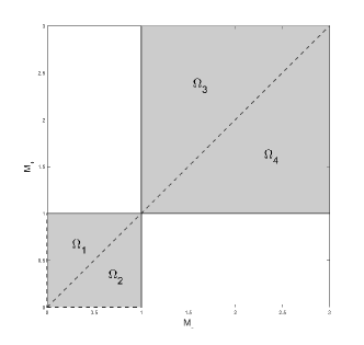
Figure 1: The admissible region of monotonicity criterion in $M_{-}-M_{+}$ graph.

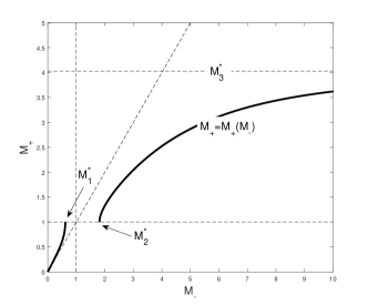
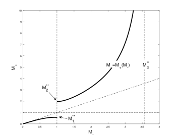
Figure 2: The function $M_{+}=M_{+}(M_{-})$ defined by (2.9). Left: $\gamma=1.4,k=0.2$. Right: $\gamma=1.4,k=-0.2$.

We first consider the case of $k>0$. A typical example of the function $M_{+}(M_{-})$ for $k>0$ is shown in the left diagram in Figure2. When $M_{-}\in\Gamma_{-}\cap(0,1]$, simple computation gives rise to

$$\lim_{M_{-}\to 0}M_{+}(M_{-})=0,$$

$$\left(M_{+}^{(1)}\right)^{-1}(1)=\begin{cases}\sqrt{\frac{k\gamma+k+1-(\gamma+1)\sqrt{k(k+1)}}{k+1-k\gamma^{2}}}<1,\ &\text{if}\ k>0,\ k\neq\frac{1}{\gamma^{2}-1}\\ \sqrt{\frac{\gamma-1}{2\gamma}}<1,\ &\text{if}\ k=\frac{1}{\gamma^{2}-1}\end{cases}.$$

When $M_{-}\in\Gamma_{-}\cap[1,+\infty)$, we assume that $k<\frac{1}{\gamma^{2}-1}$, since $M_{+}$ is unsolvable when $k\geq\frac{1}{\gamma^{2}-1}$. It follows that

$$\lim_{M_{-}\to+\infty}M_{+}(M_{-})=\sqrt{\frac{\gamma+\sqrt{1-k(\gamma^{2}-1)}}{\gamma-\gamma\sqrt{1-k(\gamma^{2}-1)}}}>1$$

$$\left(M_{+}^{(2)}\right)^{-1}(1)=\sqrt{\frac{k\gamma+k+1+(\gamma+1)\sqrt{k(k+1)}}{k+1-k\gamma^{2}}}>1$$

We use the following notations to denote these critical Mach numbers:

$$M_{1}^{*}=\begin{cases}\sqrt{\frac{k\gamma+k+1-(\gamma+1)\sqrt{k(k+1)}}{k+1-k\gamma^{2}}},\ &\text{if}\ k\neq\frac{1}{\gamma^{2}-1},\ k>0\\ \sqrt{\frac{\gamma-1}{2\gamma}},\ &\text{if}\ k=\frac{1}{\gamma^{2}-1}\end{cases}$$ (2.10)

$$M_{2}^{*}=\begin{cases}\sqrt{\frac{k\gamma+k+1+(\gamma+1)\sqrt{k(k+1)}}{k+1-k\gamma^{2}}},\ &\text{if}\ 0<k<\frac{1}{\gamma^{2}-1}\\ +\infty,\ &\text{if}\ k\geq\frac{1}{\gamma^{2}-1}\end{cases}$$

$$M_{3}^{*}=\begin{cases}\sqrt{\frac{\gamma+\sqrt{1-k(\gamma^{2}-1)}}{\gamma-\gamma\sqrt{1-k(\gamma^{2}-1)}}},\ &\text{if}\ 0<k<\frac{1}{\gamma^{2}-1}\\ +\infty,\ &\text{if}\ k\geq\frac{1}{\gamma^{2}-1}\end{cases}$$

If $k\neq 0$, then $M_{1}^{*}<M_{2}^{*}$, which implies that the solution of a stationary wave may not exist. To be precise, the left-hand state $U_{-}$ and right-hand state $U_{+}$ of a stationary wave should satisfy

$$M_{-}\in(0,M_{1}^{*}]\&M_{+}\in(0,1]\ \text{or }M_{-}\in[M_{2}^{*},\infty)\&M_{+}\in[1,M_{3}^{*}).$$

Secondly, we consider the case of $-1<k<0$. A typical example of the function $M_{+}(M_{-})$ for $-1<k<0$ is shown in the right diagram in Figure2. It is obvious that (2.2) is equivalent to

$$\begin{cases}\rho_{-}u_{-}=\rho_{+}u_{+}\left(1+\frac{-k_{1}}{1+k_{1}}\right),\\ \rho_{-}u_{-}^{2}+p_{-}=(\rho_{+}u_{+}^{2}+p_{+})\left(1+\frac{-k_{2}}{1+k_{2}}\right),\\ (E_{-}+p_{-})u_{-}=(E_{+}+p_{+})u_{+}\left(1+\frac{-k_{3}}{1+k_{3}}\right),\end{cases}$$ (2.11)

$$\frac{\left(1+\frac{-k_{1}}{1+k_{1}}\right)\left(1+\frac{-k_{3}}{1+k_{3}}\right)}{\left(1+\frac{-k_{2}}{1+k_{2}}\right)^{2}}-1=\frac{-k}{1+k}.$$

Criterion2 is symmetric for $U_{-}$ and $U_{+}$, so we are able to use all the conclusions of case $k>0$ directly with the help of transformation (2.11). Set

$$M_{1}^{**}=\sqrt{\frac{1-\sqrt{-k}}{1+\gamma\sqrt{-k}}},$$ (2.12)

$$M_{2}^{**}=\begin{cases}\sqrt{\frac{1+\sqrt{-k}}{1-\gamma\sqrt{-k}}},\ &\text{if}\ -\frac{1}{\gamma^{2}}<k<0\\ +\infty,\ &\text{if}\ -1<k\leq-\frac{1}{\gamma^{2}}\end{cases}$$

$$M_{3}^{**}=\begin{cases}\sqrt{\frac{\gamma\sqrt{1+k}+\sqrt{1+k\gamma^{2}}}{\gamma\sqrt{1+k}-\gamma\sqrt{1+k\gamma^{2}}}},\ &\text{if}\ -\frac{1}{\gamma^{2}}<k<0\\ 1,\ &\text{if}\ -1<k\leq-\frac{1}{\gamma^{2}}\end{cases}$$

A trivial verification shows that when $-1<k<0$ the left-hand state $U_{-}$ and right-hand state $U_{+}$ should satisfy

$$M_{-}\in(0,1]\&M_{+}\in(0,M_{1}^{**}]\ \text{or }M_{-}\in[1,M_{3}^{**})\&M_{+}\in[M_{2}^{**},+\infty).$$

Finally, the range of left-hand Mach number and right-hand Mach number for the case $k=0$ is

$$M_{+}=M_{-}\in(0,+\infty).$$

For given $k_{1},k_{2},k_{3}>-1$, the sets of left-hand Mach number $M_{-}$ and right-hand Mach number $M_{+}$ are shown in table1. In addition to $M_{-}=1$, we can choose the solution branch of stationary wave according to $M_{-}$. When $M_{-}=1$, it can be shown that $M_{+}^{(1)}(1)=M_{+}^{(2)}(1)$ when and only when $k=0$, which means that the solution to stationary wave is unique when $k=0$, but not when $k<0$.

Property 2.4

For the stationary wave with given left-hand state $U_{-}$ and coefficients $k_{1},k_{2},k_{3}$,

• the solution does not exist iff

  $$k>0\ \&\ M_{1}^{*}<M_{-}<M_{2}^{*}\quad\text{or}\quad k<0\ \&\ M_{-}\geq M_{3}^{**};$$

• the solution is double iff $k<0\ \&\ M_{-}=1$;

• the solution exists and is unique in other cases.

Here is a practical definition of stationary wave.

Proposition 2.2 (Stationary wave curves)

Given a left-hand state $U_{-}$, the stationary wave curve $\mathcal{D}(U_{-},k_{1},k_{2},k_{3})$ consisting of all right-hand states $U_{+}$ that can be connected to $U_{-}$ by the stationary wave with coefficients $k_{1},k_{2},k_{3}$ which satisfies Criterion1, is

$$D(U_{-},k_{1},k_{2},k_{3}): \text{if}\ k>0,\ M_{+}=\begin{cases}\sqrt{\frac{1-I}{1+\gamma I}},\ 0<M_{-}\leq M_{1}^{*}\\ \sqrt{\frac{1+I}{1-\gamma I}},\ M_{2}^{*}\leq M_{-}<+\infty\end{cases}$$

$$\text{if}\ k<0,\ M_{+}=\begin{cases}\sqrt{\frac{1-I}{1+\gamma I}},\ 0<M_{-}\leq 1\\ \sqrt{\frac{1+I}{1-\gamma I}},\ 1\leq M_{-}<M_{3}^{**}\\ \end{cases}$$

$$\text{if}\ k=0,\ M_{+}=\begin{cases}\sqrt{\frac{1-I}{1+\gamma I}},\ 0<M_{-}\leq 1\\ \sqrt{\frac{1+I}{1-\gamma I}},\ 1<M_{-}<+\infty\\ \end{cases}$$

$$\rho_{+}=\rho_{-}\left(\frac{M_{-}}{M_{+}}\right)^{2}\frac{\gamma M_{+}^{2}+1}{\gamma M_{-}^{2}+1}\frac{(1+k_{1})^{2}}{1+k_{2}},$$

$$u_{+}=u_{-}\left(\frac{M_{+}}{M_{-}}\right)^{2}\frac{\gamma M_{-}^{2}+1}{\gamma M_{+}^{2}+1}\frac{1+k_{2}}{1+k_{1}},$$

$$p_{+}=p_{-}\frac{\gamma M_{-}^{2}+1}{\gamma M_{+}^{2}+1}(1+k_{2}).$$

Here,

$$I=\frac{\sqrt{(\gamma M_{-}^{2}+1)^{2}-(\gamma+1)M_{-}^{2}[(\gamma-1)M_{-}^{2}+2](1+k)}}{\gamma M_{-}^{2}+1},$$

$k=(1+k_{1})(1+k_{3})/(1+k_{2})^{2}-1$ and $M_{1}^{*},M_{2}^{*},M_{3}^{**}$ are defined by (2.10) and (2.12).

Table 1: The $\Gamma_{-,k_{1},k_{2},k_{3}}$ and $\Gamma_{+,k_{1},k_{2},k_{3}}$ for different $k$.

$k$	subsonic branch		supersonic branch
	$\Gamma_{-}$	$\Gamma_{+}$	$\Gamma_{-}$	$\Gamma_{+}$
$(0,+\infty)$	$(0,M_{1}^{*}]$	$(0,1]$	$\left[M^{*}_{2},+\infty\right)$	$\left[1,M_{3}^{*}\right)$
${0}$	$(0,1]$	$(0,1]$	$\left[1,+\infty\right)$	$\left[1,+\infty\right)$
$(-\infty,0)$	$(0,1]$	$(0,M_{1}^{**}]$	$\left[1,M_{3}^{**}\right)$	$\left[M_{2}^{**},+\infty\right)$

By the transformation (2.11), we can directly obtain the backward wave curve of a stationary wave.

Proposition 2.3 (Stationary wave curves)

Given a right-hand state $U_{+}$, the stationary wave curve $\mathcal{D}^{B}(U_{+},k_{1},k_{2},k_{3})$ consisting of all left-hand states $U_{-}$ that can be connected to $U_{+}$ by the stationary wave with coefficients $k_{1},k_{2},k_{3}$ which satisfies Criterion1, is

$$D^{B}(U_{+},k_{1},k_{2},k_{3}): \text{if}\ k>0,\ M_{-}=\begin{cases}\sqrt{\frac{1-I^{B}}{1+\gamma I^{B}}},\ 0<M_{+}\leq 1\\ \sqrt{\frac{1+I^{B}}{1-\gamma I^{B}}},\ 1\leq M_{+}<M^{*}_{3}\\ \end{cases}$$

$$\text{if}\ k<0,\ M_{-}=\begin{cases}\sqrt{\frac{1-I^{B}}{1+\gamma I^{B}}},\ 0<M_{+}\leq M^{**}_{1}\\ \sqrt{\frac{1+I^{B}}{1-\gamma I^{B}}},\ M^{**}_{2}\leq M_{+}<+\infty\end{cases}$$

$$\text{if}\ k=0,\ M_{-}=\begin{cases}\sqrt{\frac{1-I^{B}}{1+\gamma I^{B}}},\ 0<M_{-}\leq 1\\ \sqrt{\frac{1+I^{B}}{1-\gamma I^{B}}},\ 1<M_{-}<+\infty\\ \end{cases}$$

$$\rho_{-}=\rho_{+}\left(\frac{M_{+}}{M_{-}}\right)^{2}\frac{\gamma M_{-}^{2}+1}{\gamma M_{+}^{2}+1}\frac{1+k_{2}}{(1+k_{1})^{2}},$$

$$u_{-}=u_{+}\left(\frac{M_{-}}{M_{+}}\right)^{2}\frac{\gamma M_{+}^{2}+1}{\gamma M_{-}^{2}+1}\frac{1+k_{1}}{1+k_{2}},$$

$$p_{-}=p_{+}\frac{\gamma M_{+}^{2}+1}{\gamma M_{-}^{2}+1}\frac{1}{1+k_{2}}.$$

Here,

$$I^{B}=\frac{\sqrt{(\gamma M_{+}^{2}+1)^{2}-(\gamma+1)M_{+}^{2}[(\gamma-1)M_{+}^{2}+2]/(1+k)}}{\gamma M_{+}^{2}+1},$$

$k=(1+k_{1})(1+k_{3})/(1+k_{2})^{2}-1$ and $M_{1}^{**},M_{2}^{**},M_{3}^{*}$ are defined by (2.10) and (2.12).

By the above discussion we see that

Property 2.5

The $M_{+}$ defined by (2.9) is a global monotone increasing function of $M_{-}$.

2.2 Shock waves, rarefaction waves and contact discontinuities

In this section we will introduce the elementary waves other than stationary waves, including Lax shock waves, rarefaction waves and contact discontinuities. These three elementary waves are associated with the characteristic domains of matrix $A=\partial F/\partial U$ and therefore referred to as classical elementary waves. Here we only list some conclusions to be used in this paper. For detailed introductions, we refer the reader to [43, 7].

The characteristic domains of $\lambda_{1}=u-a$ and $\lambda_{3}=u+a$ are both genuinely nonlinear. The elementary wave associated with these two characteristic domains is either a shock wave or a rarefaction wave. A Lax shock wave is the discontinuity travelling at the speed $\sigma$, the left-hand and right-hand states of which are denoted as $U_{1}$ and $U_{2}$, respectively. Subject to the Lax shock inequality([28, 29])

$$\text{1-shock: }\lambda_{1}(U_{1})>\sigma>\lambda_{1}(U_{2}),$$

$$\text{3-shock: }\lambda_{3}(U_{1})>\sigma>\lambda_{3}(U_{2}),$$

we can obtain the wave curve by the Rankine-Hugoniot condition:

$$F(U_{2})-F(U_{1})=\sigma(U_{2}-U_{1}).$$

Proposition 2.4 (Shock wave curves)

Given a left-hand state $U_{0}$, the 1-shock curve $\mathcal{S}_{1}(U_{0})$ consisting of all right-hand states $U$ that can be connected to $U_{0}$ by a Lax shock is

$$\mathcal{S}_{1}(U_{0}): \rho=\rho(p,U_{0})=\rho_{0}\frac{(\gamma-1)p_{0}+(\gamma+1)p}{(\gamma-1)p+(\gamma+1)p_{0}},\ p\geq p_{0}$$

$$u=u(p,U_{0})=u_{0}-(p-p_{0})\sqrt{\frac{1}{\rho_{0}}\frac{2}{(\gamma+1)p+(\gamma-1)p_{0}}},\ p\geq p_{0}$$

Given a right-hand state $U_{0}$, the 3-shock curve $\mathcal{S}_{3}(U_{0})$ consisting of all left-hand states $U$ that can be connected to $U_{0}$ by a Lax shock is

$$\mathcal{S}_{3}(U_{0}): \rho=\rho(p,U_{0})=\rho_{0}\frac{(\gamma-1)p_{0}+(\gamma+1)p}{(\gamma-1)p+(\gamma+1)p_{0}},\ p\geq p_{0}$$

$$u=u(p,U_{0})=u_{0}+(p-p_{0})\sqrt{\frac{1}{\rho_{0}}\frac{2}{(\gamma+1)p+(\gamma-1)p_{0}}},\ p\geq p_{0}$$

A rarefaction wave is a piecewise smooth self-similar solution. The Riemann invariants across the 1-rarefaction and 3-rarefaction are

$$u+\frac{2a}{\gamma-1}=\text{constant},\ s=\text{constant}(\text{across}\ \lambda_{1}),$$

$$u-\frac{2a}{\gamma-1}=\text{constant},\ s=\text{constant}(\text{across}\ \lambda_{3}),$$

where $s$ is the entropy. Then we can get the wave curve of rarefaction waves.

Proposition 2.5 (Rarefaction wave curves)

Given a left-hand state $U_{0}$, the 1-rarefaction curve $\mathcal{R}_{1}(U_{0})$ consisting of all right-hand states $U$ that can be connected to $U_{0}$ by a rarefaction wave is

$$\mathcal{R}_{1}(U_{0}): \rho=\rho(p,U_{0})=\rho_{0}\left(\frac{p}{p_{0}}\right)^{\frac{1}{\gamma}},\ p\leq p_{0}$$

$$u=u(p,U_{0})=u_{0}-\frac{2a_{0}}{\gamma-1}\left[\left(\frac{p}{p_{0}}\right)^{\frac{\gamma-1}{2\gamma}}-1\right],\ p\leq p_{0}$$

Given a right-hand state $U_{0}$, the 3-rarefaction curve $\mathcal{S}_{3}(U_{0})$ consisting of all left-hand states $U$ that can be connected to $U_{0}$ by a rarefaction wave is

$$\mathcal{R}_{3}(U_{0}): \rho=\rho(p,U_{0})=\rho_{0}\left(\frac{p}{p_{0}}\right)^{\frac{1}{\gamma}},\ p\leq p_{0}$$

$$u=u(p,U_{0})=u_{0}+\frac{2a_{0}}{\gamma-1}\left[\left(\frac{p}{p_{0}}\right)^{\frac{\gamma-1}{2\gamma}}-1\right],\ p\leq p_{0}$$

The characteristic domain of $\lambda_{2}=u$ is linearly degenerate. The elementary wave associated with the $\lambda_{2}$ characteristic domain is the contact discontinuity.

Proposition 2.6 (contact discontinuity curves)

Given a left-hand state $U_{0}$, the 2-contact discontinuity curve $\mathcal{R}_{1}(U_{0})$ consisting of all right-hand states $U$ that can be connected to $U_{0}$ by a contact discontinuity is

$$\mathcal{C}_{2}(U_{0}):\ u=u_{0},\ p=p_{0}.$$

3 Structures of Riemann solution

The Riemann problem is a Cauchy problem of (1.1) with piecewise constant initial conditions:

$$\left\{\begin{aligned} &\frac{\partial U}{\partial t}+\frac{\partial F}{\partial x}=\delta(x)S,\\ &U(x,0)=\begin{cases}U_{L},\ x<0\\ U_{R},\ x>0\end{cases}\end{aligned}\right.$$ (3.1)

The Riemann problem of classical Euler equations with the same initial value, which is also called associate Riemann problem, is

$$\left\{\begin{aligned} &\frac{\partial U}{\partial t}+\frac{\partial F}{\partial x}=0,\\ &U(x,0)=\begin{cases}U_{L},\ x<0\\ U_{R},\ x>0\end{cases}\end{aligned}\right.$$ (3.2)

The solution of the associative Riemann problem (3.2) is self-similar and contains four constant regions, which are divided by three classical elementary waves, as shown in the left figure of Figure3. Although the governing equation (1.1) contains source terms, it is clearly still self-similar, thus we only consider self-similar solutions of the Riemann problem (3.1). The following assumption will be needed throughout the paper.

Assumption 3.1

The solutions of Riemann problem (3.1) is self-similar

$$U(x,t)=U\left(\frac{x}{t}\right).$$

The self-similar solution of Riemann problem (3.1) and associate Riemann problem (3.2) with the initial value condition $U_{L}$ and $U_{R}$ are denoted as $U^{R}\left(\frac{x}{t},U_{L},U_{R}\right),\ U^{A-R}\left(\frac{x}{t},U_{L},U_{R}\right)$, respectively. Under Assumption3.1, $U_{-}=U^{R}\left(\frac{x}{t}=0-,U_{L},U_{R}\right)$ and $U_{+}=U^{R}\left(\frac{x}{t}=0+,U_{L},U_{R}\right)$ are both time-independent vectors.

Double classical Riemann problem(CRP) framework will be used to analyze the structures of Riemann solutions in this section.

Proposition 3.1 (Double CRP framework)

The self-similar solution of the Riemann problem consists of seven discontinuities at most. They are a stationary wave at $x=0$, two genuinely nonlinear waves and a contact discontinuity left to $x=0$, two genuinely nonlinear waves and a contact discontinuity right to $x=0$ respectively.

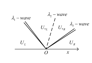
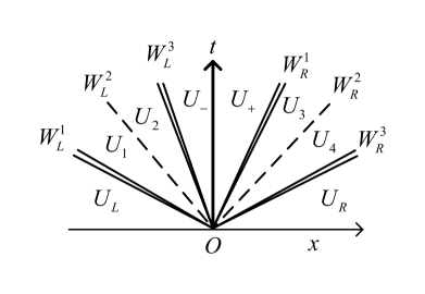
Figure 3: The general structure of Riemann solutions. Left: associate Riemann problem (3.1). Right: Riemann problem (3.2).

According to Proposition3.1, the general structure of Riemann solutions is shown in the right figure of Figure3. The elementary waves on the left and right sides are denoted as $W_{L}^{1}$, $W_{L}^{2}$, $W_{L}^{3}$ and $W_{R}^{1}$, $W_{R}^{2}$, $W_{R}^{3}$, respectively. $W_{L}^{1}$, $W_{L}^{3}$, $W_{R}^{1}$ and $W_{R}^{3}$ can be shock waves or rarefaction waves, and both $W_{L}^{2}$ and $W_{R}^{2}$ are contact discontinuities. The t-axis is a stationary wave and $U_{-}\neq U_{+}$. We follow the notation of [32, 41] to express the structure of Riemann solutions. For example, $\mathcal{S}(U_{L},U_{1})$ and $\mathcal{R}(U_{L},U_{1})$ mean that two states $U_{L}$ and $U_{1}$ are connected by a shock and a rarefaction wave, respectively. The symbol $\mathcal{W}(U_{L},U_{1})$ means that $U_{L}$ and $U_{1}$ are connected by a shock wave or a rarefaction wave. $\mathcal{C}(U_{1},U_{2})$ means that $U_{1}$ and $U_{2}$ are connected by a contact discontinuity, and $\mathcal{D}(U_{-},U_{+})$ means that $U_{-}$ and $U_{+}$ are connected by a stationary wave. The connection between multiple elementary waves and constant regions is represented by the symbol ”$\oplus$”. For example, $\mathcal{S}(U_{L},U_{1})\oplus\mathcal{C}(U_{1},U_{2})$ means that $U_{L}$ and $U_{1}$ are connected by a shock and a shock wave, followed by a contact discontinuity with the left-hand state $U_{1}$ and the right-hand state $U_{2}$.

Theorem 3.1

There are seven structures of the Riemann solution:

• non-choked structures:

  • Type1: $\mathcal{W}(U_{L},U_{-})\oplus\mathcal{D}(U_{-},U_{+})\oplus\mathcal{C}(U_{+},U_{4})\oplus\mathcal{W}(U_{4},U_{R})$.

  • Type2: $\mathcal{D}(U_{L},U_{+})\oplus\mathcal{W}(U_{+},U_{3})\oplus\mathcal{C}(U_{3},U_{4})\oplus\mathcal{W}(U_{4},U_{R})$.

• choked structures:

  • Type3: $\mathcal{W}(U_{L},U_{-})\oplus\mathcal{D}(U_{-},U_{+})\oplus\mathcal{R}(U_{+},U_{3})\oplus\mathcal{C}(U_{3},U_{4})\oplus\mathcal{W}(U_{4},U_{R})$ with $M_{+}=1$.

  • Type4: $\mathcal{D}(U_{L},U_{+})\oplus\mathcal{R}(U_{+},U_{3})\oplus\mathcal{C}(U_{3},U_{4})\oplus\mathcal{W}(U_{4},U_{R})$ with $M_{+}=1$.

  • Type5: $\mathcal{R}(U_{L},U_{-})\oplus\mathcal{D}(U_{-},U_{+})\oplus\mathcal{W}(U_{+},U_{3})\oplus\mathcal{C}(U_{3},U_{4})\oplus\mathcal{W}(U_{4},U_{R})$ with $M_{-}=1$.

  • Type6: $\mathcal{R}(U_{L},U_{-})\oplus\mathcal{D}(U_{-},U_{+})\oplus\mathcal{C}(U_{+},U_{4})\oplus\mathcal{W}(U_{4},U_{R})$ with $M_{-}=1$.

  • Type7: $\mathcal{R}(U_{L},U_{-})\oplus\mathcal{D}(U_{-},U_{+})\oplus\mathcal{R}(U_{+},U_{3})\oplus\mathcal{C}(U_{3},U_{4})\oplus\mathcal{W}(U_{4},U_{R})$ with $M_{-}=M_{+}=1$.

Proof 3.1

Following the idea of double CRP framework, we first give the relations between the waves in the left and right half-planes with respect to states $U_{-}$ and $U_{+}$ respectively, and then combine these two sets of waves to form the structure of global Riemann solution under Criterion1.

We begin by considering the structure of the left half-plane.

We use a contradiction to prove that the wave $W_{L}^{3}$ do not exist. If the assertion would not hold, then it follows from $u_{-}+a_{-}>u_{-}>0$ that $W_{L}^{3}$ cannot be a rarefaction wave, therefore $W_{L}^{3}$ is a shock wave. Let $\sigma_{L,3}$ denotes the speed of $W_{L}^{3}$. It follows from Lax entropy condition that $\sigma_{L,3}>u_{-}+a_{-}>0$, which contradicts $\sigma_{L,3}<0$. We have proved that $W_{L}^{3}$ does not exist, then it follows from $u_{-}>0$ that the wave $W_{L}^{2}$ does not exist either.

We now consider the wave $W_{L}^{1}$ in the following three cases.

First, if $0<M_{-}<1$, then it is clear that wave $W_{L}^{1}$ is possible in the solution.

Second, if $M_{-}>1$, then we assert that $W_{L}^{1}$ does not exist. Otherwise, if $W_{L}^{1}$ exists, then it must be a shock wave with negative speed. Let $\sigma_{L,1}$ denotes the speed of $W_{L}^{1}$. According to Lax entropy condition, we have $0>\sigma_{L,1}>u_{-}-a_{-}>0$, which is impossible.

Finally, if $M_{-}=1$, then we assert that $W_{L}^{1}$ is a rarefaction wave. If $W_{L}^{1}$ exists and is a shock wave, then Lax entropy condition shows that $\sigma_{L,1}>u_{-}-a_{-}=0$, which is contrary to $\sigma_{L,1}\leq 0$. In addition, the nonexistence of $W_{L}^{1}$ can be regarded as the degeneration of a rarefaction wave, hence $W_{L}^{1}$ is a rarefaction wave.

We have thus related the structure of left half-plane to the value of $M_{-}$ as follows.

• If $0<M_{-}<1$, then the Riemann solution contains only a classical nonlinear wave $W_{L}^{1}$ in the left half-plane.

• If $M_{-}=1$, then the Riemann solution contains only a rarefaction wave $W_{L}^{1}$ in the left half-plane.

• If $M_{-}>1$, then the Riemann solutions do not contain waves in the left half-plane.

Using a similar approach, we can then prove the relations between elementary waves and $U_{+}$ in the right half-plane as follows.

• If $0<M_{+}<1$, then the structure of Riemann solution in the right half-plane is $\mathcal{C}(U_{+},U_{4})\oplus\mathcal{W}(U_{4},U_{R})$.

• If $M_{+}=1$, then the structure of Riemann solution in the right half-plane is $\mathcal{W}(U_{+},U_{3})\oplus\mathcal{C}(U_{3},U_{4})\oplus\mathcal{W}(U_{4},U_{R})$.

• If $M_{+}>1$, then the structure of Riemann solution in the right half-plane is $\mathcal{R}(U_{+},U_{3})\oplus\mathcal{C}(U_{3},U_{4})\oplus\mathcal{W}(U_{4},U_{R})$.

The final step of the proof is to couple the left and right parts of elementary waves under Criterion2. According to Criterion2, there are two cases of $M_{-}$ and $M_{+}$ for non-choked structures. If $0<M_{-},M_{+}<1$, the structure of solution is

$$\mathcal{W}(U_{L},U_{-})\oplus\mathcal{D}(U_{-},U_{+})\oplus\mathcal{C}(U_{+},U_{4})\oplus\mathcal{W}(U_{4},U_{R}).$$

If $M_{-},M_{+}>1$, the structure of solution is

$$\mathcal{D}(U_{L},U_{+})\oplus\mathcal{W}(U_{+},U_{3})\oplus\mathcal{C}(U_{3},U_{4})\oplus\mathcal{W}(U_{4},U_{R}).$$

The structure of choked solution is different for different signs of $k$. When $k>0$, it follows from 1 that $M_{-}=M_{1}^{*},M_{+}=1$ or $M_{-}=M_{2}^{*},M_{+}=1$, then the two structures of choked solution are

$$\mathcal{W}(U_{L},U_{-})\oplus\mathcal{D}(U_{-},U_{+})\oplus\mathcal{R}(U_{+},U_{3})\oplus\mathcal{C}(U_{3},U_{4})\oplus\mathcal{W}(U_{4},U_{R}),$$

$$\mathcal{D}(U_{L},U_{+})\oplus\mathcal{R}(U_{+},U_{3})\oplus\mathcal{C}(U_{3},U_{4})\oplus\mathcal{W}(U_{4},U_{R}).$$

When $k<0$, the choked solution satisfies $M_{-}=1,M_{+}=M_{1}^{**}$ or $M_{-}=1,M_{+}=M_{2}^{**}$, and its structures are

$$\mathcal{R}(U_{L},U_{-})\oplus\mathcal{D}(U_{-},U_{+})\oplus\mathcal{W}(U_{+},U_{3})\oplus\mathcal{C}(U_{3},U_{4})\oplus\mathcal{W}(U_{4},U_{R}),$$

$$\mathcal{R}(U_{L},U_{-})\oplus\mathcal{D}(U_{-},U_{+})\oplus\mathcal{C}(U_{+},U_{4})\oplus\mathcal{W}(U_{4},U_{R}).$$

When $k=0$, the choked solution satisfies $M_{-}=M_{+}=1$, and its structure is

$$\mathcal{R}(U_{L},U_{-})\oplus\mathcal{D}(U_{-},U_{+})\oplus\mathcal{R}(U_{+},U_{3})\oplus\mathcal{C}(U_{3},U_{4})\oplus\mathcal{W}(U_{4},U_{R}).$$

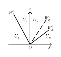
(a) Type1

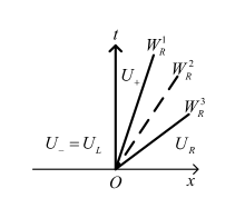
(b) Type2

Figure 4: The non-choked structures of Riemann solutions.

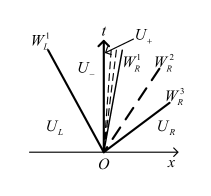
(a) Type3

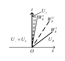
(b) Type4

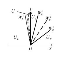
(c) Type5

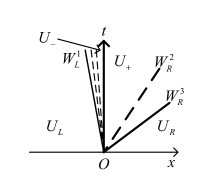
(d) Type6

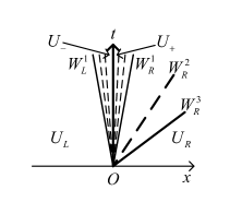
(e) Type7

Figure 5: The choked structures of Riemann solutions.

The sketches of these seven structures are shown in FigureLABEL:figure:_non-choked_structures,figure:_choked_structures. The non-choked structure is in the form of a stationary wave bisecting a certain constant region of a classical Riemann solution, and these two new regions satisfy the jump relation equation (2.1). The choked structure is more complex, where the elementary wave associated with a certain characteristic domain appears twice, and one of these two waves is a rarefaction wave and in contact with the stationary wave. From the proof of Thoerem3.1 we have obtained all possible structures of Riemann solutions for the three ranges of coefficients $k$, as follows.

Corollary 3.1

• If $k>0$, then all possible structures of the Riemann solutions are Type1, Type2, Type3 and Type4.

• If $k<0$, then all possible structures of the Riemann solutions are Type1, Type2, Type5 and Type6.

• If $k=0$, then all possible structures of the Riemann solutions are Type1, Type2 and Type7.

The possible structures of solutions for different $k$ and their corresponding ranges of Mach numbers on either side of stationary wave are shown in table2.

Table 2: For each $k$, the possible structure of the Riemann solution and the range of Mach numbers on both sides of the stationary wave.

Coefficients	Solution structure	Upstream Mach number	Downstream Mach number
$k>0$	Type1	$0<M_{-}<M^{*}_{1}$	$0<M_{+}<1$
	Type2	$M_{-}>M^{*}_{2}$	$1<M_{+}<M^{*}_{3}$
	Type3	$M_{-}=M^{*}_{1}$	$M_{+}=1$
	Type4	$M_{-}=M^{*}_{2}$	$M_{+}=1$
$k<0$	Type1	$0<M_{-}<1$	$0<M_{+}<M^{**}_{1}$
	Type2	$1<M_{-}<M^{**}_{3}$	$M_{+}>M^{**}_{2}$
	Type5	$M_{-}=1$	$M_{+}=M^{**}_{1}$
	Type6	$M_{-}=1$	$M_{+}=M^{**}_{2}$
$k=0$	Type1	$0<M_{-}<1$	$0<M_{+}<1$
	Type2	$M_{-}>1$	$M_{+}>1$
	Type7	$M_{-}=1$	$M_{+}=1$

In some special cases, there are two admissible branches of the wave curve of the stationary wave. We show below that it does not lead to the Riemann problem being ill-posed.

The case of multiple solutions of the wave curve 2.2 satisfies

$$k>0,M_{-}=M_{1}^{*}\text{ or }M_{1}^{**},M_{+}=1.$$ (3.3)

Property 3.1

Suppose the initial values of the Riemann solution $U_{1}(x,t)$ are $U_{L,1}$ and $U_{R,1}$ and $M_{-}=M_{1}^{*},M_{+}=1$ are satisfied, and the initial values of the Riemann solution $U_{2}(x,t)$ are $U_{L,2}$ and $U_{R,2}$ and $M_{-}=M_{1}^{**},M_{+}=1$ are satisfied. If $U_{L,1}=U_{L,2},U_{R,1}=U_{R,2}$, then

$$U_{1}(x,t)=U_{2}(x,t),\forall x\in\mathbb{R},t\geq 0.$$

Proof 3.2

The structure of $U_{1}$ is Type3, and the structure of $U_{2}$ is Type4. If $U_{L,1}=U_{L,2}$, then $M_{L,1}=M_{1}^{**}$.

For $U_{1}$, we have $M_{-}=M_{1}^{*}$. From the fact that $M_{1}^{*}$ and $M_{1}^{**}$ satisfy the Prandtl relation

$$(M_{1}^{**})^{2}=\frac{1+[(\gamma-1)/2(M_{1}^{*})^{2}]}{\gamma(M_{1}^{*})^{2}-(\gamma-1)/2}$$

we know that the wave $W_{L}^{1}$ is a normal shock wave, therefore

$$U_{1}(x,t)=U_{2}(x,t)\equiv U_{L},\forall x<0,t\geq 0.$$

By $U_{1}(0+,t)=U_{2}(0+,t)$ and the uniqueness of classical Riemann solution, we have

$$U_{1}(x,t)=U_{2}(x,t),\forall x>0,t\geq 0.$$

The case of multiple solutions of the wave curve Proposition2.3 satisfies

$$k<0,M_{-}=1,M_{+}=M_{2}^{*}\text{ or }M_{2}^{**}.$$ (3.4)

Property 3.2

Suppose the initial values of the Riemann solution $U_{1}(x,t)$ are $U_{L,1}$ and $U_{R,1}$ and $M_{-}=1,M_{+}=M_{2}^{*}$ are satisfied, and the initial values of the Riemann solution $U_{2}(x,t)$ are $U_{L,2}$ and $U_{R,2}$ and $M_{-}=1,M_{+}=M_{2}^{**}$ are satisfied. If $U_{L,1}=U_{L,2},U_{R,1}=U_{R,2}$, then

$$U_{1}(x,t)=U_{2}(x,t),\forall x\in\mathbb{R},t\geq 0.$$

The proof of this result is quite similar to that of Property3.1 and so is omitted. Property3.1 and Property3.2 show that the multiple admissible branches of stationary wave curves do not lead to the multiple solutions of the Riemann problem.

4 Conclusions

The Riemann problem of Euler equations with a singular source was studied. We proposed an eigenvalue-based monotonicity criterion for selecting the physical solution of stationary waves. The criterion is also valid for singular source-induced discontinuities in other equations, such as the shallow water equations. We analyzed all possible structures of Riemann solution under the double CRP framework. The theoretical conclusions in this paper on the stationary wave and the Riemann problem are very helpful in the design of numerical schemes, and the related work will be given in a subsequent paper.

References

- [1] Remi Abgrall, P Bacigaluppi, and S Tokareva. A high-order nonconservative approach for hyperbolic equations in fluid dynamics. Computers & Fluids, 169:10–22, 2018.
- [2] Rémi Abgrall and Smadar Karni. A comment on the computation of non-conservative products. Journal of Computational Physics, 229(8):2759–2763, 2010.
- [3] Francisco Alcrudo and Fayssal Benkhaldoun. Exact solutions to the riemann problem of the shallow water equations with a bottom step. Computers & Fluids, 30(6):643–671, 2001.
- [4] John David Anderson. Modern compressible flow: with historical perspective, volume 12. McGraw-Hill New York, 1990.
- [5] Roberto Bernetti, Vladimir A Titarev, and Eleuterio F Toro. Exact solution of the riemann problem for the shallow water equations with discontinuous bottom geometry. Journal of Computational Physics, 227(6):3212–3243, 2008.
- [6] Manuel J Castro, Alberto Pardo Milanés, and Carlos Parés. Well-balanced numerical schemes based on a generalized hydrostatic reconstruction technique. Mathematical Models and Methods in Applied Sciences, 17(12):2055–2113, 2007.
- [7] Tung Chang and Ling Hsiao. The riemann problem and interaction of waves in gas dynamics. NASA STI/Recon Technical Report A, 90:44044, 1989.
- [8] Wan Cheng, Xisheng Luo, and MEH Van Dongen. On condensation-induced waves. Journal of fluid mechanics, 651:145–164, 2010.
- [9] Frédéric Coquel, Khaled Saleh, and Nicolas Seguin. A robust and entropy-satisfying numerical scheme for fluid flows in discontinuous nozzles. Mathematical Models and Methods in Applied Sciences, 24(10):2043–2083, 2014.
- [10] Pratik Das and HS Udaykumar. A sharp-interface method for the simulation of shock-induced vaporization of droplets. Journal of Computational Physics, 405:109005, 2020.
- [11] Pratik Das and HS Udaykumar. A simulation-derived surrogate model for the vaporization rate of aluminum droplets heated by a passing shock wave. International Journal of Multiphase Flow, 130:103299, 2020.
- [12] Pratik Das and HS Udaykumar. Sharp-interface calculations of the vaporization rate of reacting aluminum droplets in shocked flows. International Journal of Multiphase Flow, 134:103442, 2021.
- [13] Can F Delale, Günter H Schnerr, and Marinus EH van Dongen. Condensation discontinuities and condensation induced shock waves. In Shock Wave Science and Technology Reference Library, pages 187–230. Springer, 2007.
- [14] Mehv Dongen, X. Luo, G. Lamanna, and Djv Kaathoven. On condensation induced shock waves. In Proc. 10th Chinese Symposium on Shock Waves, 2002.
- [15] Michael Dumbser. A diffuse interface method for complex three-dimensional free surface flows. Computer Methods in Applied Mechanics and Engineering, 257:47–64, 2013.
- [16] Stefan Fechter, Claus-Dieter Munz, Christian Rohde, and Christoph Zeiler. Approximate riemann solver for compressible liquid vapor flow with phase transition and surface tension. Computers & Fluids, 169:169–185, 2018.
- [17] Paola Goatin and Philippe G LeFloch. The riemann problem for a class of resonant hyperbolic systems of balance laws. Annales de l’Institut Henri Poincaré (C) Non Linear Analysis, 21(6):881–902, 2004.
- [18] L Gosse. A well-balanced flux-vector splitting scheme designed for hyperbolic systems of conservation laws with source terms. Computers & Mathematics with Applications, 39(9-10):135–159, 2000.
- [19] Laurent Gosse. A well-balanced scheme using non-conservative products designed for hyperbolic systems of conservation laws with source terms. Mathematical Models and Methods in Applied Sciences, 11(02):339–365, 2001.
- [20] JM Greenberg, AY Leroux, R Baraille, and A Noussair. Analysis and approximation of conservation laws with source terms. SIAM Journal on Numerical Analysis, 34(5):1980–2007, 1997.
- [21] Joshua M Greenberg and Alain-Yves LeRoux. A well-balanced scheme for the numerical processing of source terms in hyperbolic equations. SIAM Journal on Numerical Analysis, 33(1):1–16, 1996.
- [22] Timon Hitz, Matthias Heinen, Jadran Vrabec, and Claus-Dieter Munz. Comparison of macro-and microscopic solutions of the riemann problem i. supercritical shock tube and expansion into vacuum. Journal of Computational Physics, 402:109077, 2020.
- [23] T. Y. Hou and P. G. Lefloch. Why nonconservative schemes converge to wrong solutions: error analysis. Math. Comp., 1994.
- [24] Ryan W Houim and Kenneth K Kuo. A ghost fluid method for compressible reacting flows with phase change. Journal of Computational Physics, 235:865–900, 2013.
- [25] Shi Jin. A steady-state capturing method for hyperbolic systems with geometrical source terms. ESAIM: Mathematical Modelling and Numerical Analysis, 35(4):631–645, 2001.
- [26] Dietmar Kröner, Philippe G LeFloch, and Mai-Duc Thanh. The minimum entropy principle for compressible fluid flows in a nozzle with discontinuous cross-section. ESAIM: Mathematical Modelling and Numerical Analysis, 42(3):425–442, 2008.
- [27] Dietmar Kröner and Mai Duc Thanh. Numerical solutions to compressible flows in a nozzle with variable cross-section. SIAM journal on numerical analysis, 43(2):796–824, 2005.
- [28] Peter D Lax. Hyperbolic systems of conservation laws ii. Communications on pure and applied mathematics, 10(4):537–566, 1957.
- [29] Peter D Lax. Hyperbolic systems of conservation laws and the mathematical theory of shock waves. SIAM, 1973.
- [30] Philippe Le Floch. Shock waves for nonlinear hyperbolic systems in nonconservative form. 1989.
- [31] Jaewon Lee and Gihun Son. A sharp-interface level-set method for compressible bubble growth with phase change. International Communications in Heat and Mass Transfer, 86:1–11, 2017.
- [32] Philippe G Lefloch and Mai Duc Thanh. The riemann problem for fluid flows in a nozzle with discontinuous cross-section. Communications in Mathematical Sciences, 1(4):763–797, 2003.
- [33] Philippe G LeFloch and Mai Duc Thanh. A godunov-type method for the shallow water equations with discontinuous topography in the resonant regime. Journal of Computational Physics, 230(20):7631–7660, 2011.
- [34] Philippe G LeFloch, Mai Duc Thanh, et al. The riemann problem for the shallow water equations with discontinuous topography. Communications in Mathematical Sciences, 5(4):865–885, 2007.
- [35] Gang Li, Jiaojiao Li, Shouguo Qian, and Jinmei Gao. A well-balanced ader discontinuous galerkin method based on differential transformation procedure for shallow water equations. Applied Mathematics and Computation, 395:125848, 2021.
- [36] Tian Long, Jinsheng Cai, and Shucheng Pan. A fully conservative sharp-interface method for compressible mulitphase flows with phase change. arXiv preprint arXiv:2110.07995, 2021.
- [37] Carlos Parés. Numerical methods for nonconservative hyperbolic systems: a theoretical framework. SIAM Journal on Numerical Analysis, 44(1):300–321, 2006.
- [38] Carlos Parés and Ernesto Pimentel. The riemann problem for the shallow water equations with discontinuous topography: The wet–dry case. Journal of Computational Physics, 378:344–365, 2019.
- [39] Thomas Paula, Stefan Adami, and Nikolaus A Adams. Analysis of the early stages of liquid-water-drop explosion by numerical simulation. Physical Review Fluids, 4(4):044003, 2019.
- [40] GH Schnerr. Unsteadiness in condensing flow: dynamics of internal flows with phase transition and application to turbomachinery. Proceedings of the Institution of Mechanical Engineers, Part C: Journal of Mechanical Engineering Science, 219(12):1369–1410, 2005.
- [41] Mai Duc Thanh. The riemann problem for a nonisentropic fluid in a nozzle with discontinuous cross-sectional area. SIAM Journal on Applied Mathematics, 69(6):1501–1519, 2009.
- [42] Mai Duc Thanh and Dao Huy Cuong. Properties of the wave curves in the shallow water equations with discontinuous topography. Bulletin of the Malaysian Mathematical Sciences Society, 39(1):305–337, 2016.
- [43] Eleuterio F Toro. Riemann solvers and numerical methods for fluid dynamics: a practical introduction. Springer Science & Business Media, 2013.
- [44] Yang Yang and Chi-Wang Shu. Discontinuous galerkin method for hyperbolic equations involving delta-singularities: negative-order norm error estimates and applications. Numerische Mathematik, 124(4):753–781, 2013.
- [45] Changsheng Yu, Chengliang Feng, Zhiqiang Zeng, and Tiegang Liu. Riemann problem for constant flow with single-point heating source. arXiv preprint arXiv:2203.03155, 2022.
- [46] Changsheng Yu, Tiegang Liu, and Chengliang Feng. Waves induced by the appearance of single-point heat source in constant flow. ADVANCES IN APPLIED MATHEMATICS AND MECHANICS, 2021.