Ground and excited states of coupled exciton liquids in electron-hole quadrilayers

Abstract

Interlayer excitons are bound states of electrons and holes confined in separate two-dimensional layers. Due to their repulsive dipolar interaction, interlayer excitons can form a correlated liquid. If another electron-hole bilayer is present, excitons from different bilayers can exhibit mutual attraction. We study such a quadrilayer system by a hypernetted chain formalism. We compute ground state energies, pair correlation functions, and collective mode velocities as functions of the exciton densities. We estimate the critical density for the transition to a paired biexciton phase. For a strongly unbalanced (unequal density) system, the excitons in the more dilute bilayer behave as polarons. We compute energies and effective masses of such exciton-polarons.

I Introduction

Indirect exciton or equivalently, interlayer exciton is a neutral quasi-particle in a semiconductor nanostructure that contains two parallel layers: one, filled with electrons and the other, with holes. An interlayer exciton can be created by a photoexcitation of an electron-hole (e-h) pair followed by separation of the two particles via interlayer tunneling induced by a strong out-of-plane electric field. Low-disorder $\rm{GaAs}$-based nanostructures have proved to be particularly suitable for realization of interlayer exciton systems with tunable density, long lifetime Lozovik and Yudson (1976); Butov et al. (2001), high mobility Dorow et al. (2018), and long diffusion length Hagn et al. (1995); Gärtner et al. (2006); Hammack et al. (2009); Leonard et al. (2009); Lazić et al. (2010); Alloing et al. (2012); Lazić et al. (2014); Finkelstein et al. (2017). In a theoretical analysis of such systems it has been common to treat excitons as composite bosons with no internal dynamics. (Henceforth, “exciton” always means interlayer exciton.) In this approximation each exciton has a permanent dipole moment proportional to the separation of the electron and hole layers. The interaction of such oriented dipoles located in the same two-dimensional (2D) plane is strictly repulsive.

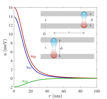
Figure 1: Exciton interaction potentials: $u_{11}$ and $u_{22}$ are intraplane potentials; $u_{12}$ is the interplane potential. The inset shows a schematic of the system (see text). Parameters: $d_{1}=20\,\mathrm{nm}$, $d_{2}=25\,\mathrm{nm}$, $D=43\,\mathrm{nm}$, $\kappa=13$, $c=5\,\mathrm{nm}$.

Recent experiments Hubert et al. (2019); Choksy et al. (2021) explored a more advanced type of $\rm{GaAs}/{\rm{Ga}}{\rm{Al}}{\rm{As}}$ nanostructures containing two e-h bilayers, as shown schematically in Fig. 1. In these e-h-e-h quadrilayer systems, the dipolar interaction between excitons that belong to different e-h bilayers can be of either sign. This interaction is repulsive at large but attractive at small in-plane distances $r$ between the excitons, see the curve labeled $u_{12}$ in Fig. 1. Experimental evidence for the interlayer attraction Hubert et al. (2019); Choksy et al. (2021) was deduced from the dependence of the exciton photoluminescence energy and the exciton density distribution Choksy et al. (2021) on the separately controlled average exciton densities in the two bilayers. Motivated by these experiments, in this paper we undertake a quantitative analysis of the ground state and excitations of an e-h-e-h quadrilayer system.

Our study is a continuation of extensive prior theoretical work on e-h bilayers and 2D dipolar bosons. For example, the phase diagram of a single e-h bilayer for the case where electrons and holes have equal densities $n$ and masses $m_{e}=m_{h}$ has been explored by several Monte-Carlo simulations De Palo et al. (2002); Tan et al. (2005); Lee et al. (2009); Maezono et al. (2013). Such simulations are considered to be the most reliable tool for the case of strong correlations. These studies have shown that the excitons are stable when $n$ is below a certain threshold (Mott critical density) $n_{c2}=c_{2}a_{e}^{-2}$. Here $c_{2}\sim 0.02$ is a numerical coefficient that depends on the dimensionless ratio $d/a_{e}$ of the e-h separation $d$ and the electron Bohr radius $a_{e}=\hbar^{2}\kappa/m_{e}e_{0}^{2}$ with $\kappa$ and $e_{0}$ being the dielectric constant and the elementary charge, respectively. Neglecting internal dynamics of excitons is justified if $n\ll n_{c2}$. The ground state of the system is determined by the competition between the kinetic energy of the excitons and their dipole repulsion that scales as $d^{2}$. In the experimentally relevant regime Hubert et al. (2019); Choksy et al. (2021) $d/a_{e}\sim 0.3$, excitons are expected to form a strongly correlated Bose liquid (which is a superfluid). At much larger or much smaller $d$’s, other phases of exciton matter, e.g., exciton solid are possible.

Phase diagram of 2D dipolar bosons inferred from Monte-Carlo simulations shows a close correspondence to that of the e-h bilayer in regards to the position of the liquid-solid phase boundary Astrakharchik et al. (2007, 2008); Büchler et al. (2007). Numerical results for the ground-state energy and density correlation function of 2D dipolar bosons have been conveniently summarized in Astrakharchik et al. (2009) and we will use some of them in this work. The excitation spectra of such systems Astrakharchik et al. (2007); Hufnagl et al. (2011); Abedinpour et al. (2012) have also been studied. Additional work in this subject area includes investigations of the thermal melting of dipolar solids Mora et al. (2007) and the scattering-length instability Bortolotti et al. (2006). The latter has implications for the normal-superfluid transition. For systems of dipoles whose orientation is tilted away from the vertical, a unidirectional density wave (stripe) phase was predicted to appear Macia et al. (2012, 2014a).

The most directly relevant to our work are Monte-Carlo simulations done for bilayer systems of magnetic dipolar bosons Macia et al. (2014b); Filinov (2016); Cinti et al. (2017), which have essentially the same interaction law as excitons. Based on these studies, we can surmise the following structure of the zero-temperature phase diagrams of e-h-e-h quadrilayers. To avoid confusion we will use the term “plane” in relation to excitons and “layer” for electrons or holes. (Hence, a plane is made of a pair of adjacent layers.) Let us start with a symmetric case, i.e., two parallel planes each filled with excitons of dipole moment $e_{0}d$ and density $n$. The planes are separated by a distance $D>d$. The dimensionless parameters of the problem are obtained by multiplying $D$, $n$, and $d$ by appropriate powers of the dipole length $a=d^{2}/a_{x}$, where $a_{x}=\hbar^{2}\kappa/me_{0}^{2}=a_{e}m_{e}/m$ is the effective exciton Bohr radius and $m=m_{e}+m_{h}$ is the exciton mass. As shown schematically in Fig. 2(a), if $D/a$ and $na^{2}$ are small, so that the mean in-plane exciton distance $n^{-1/2}$ is relatively large, the interplane attraction of excitons favors paired phases. This means that excitons from the opposite planes bind into biexcitons if $n$ is less than some critical density $n_{c1}=n_{c1}(D)$. The biexcitons would typically form a correlated liquid but a small region of the solid phase is also possible. When $D/a$ or $na^{2}$ is large, the intraplane repulsion dominates over the interplane attraction, so that the unpaired exciton fluids are stable. However, the excitons should dissociate once $n$ increases beyond the Mott critical density, which is the rightmost part of the phase diagram. The rectilinear phase boundaries in Fig. 2(a) are meant to be schematic only.

In principle, more exotic phases of matter are possible in this system. For example, intraplane exchange interaction and spin-related effects can become important at high exciton density. In this paper, we focus on the moderate and low-density regimes, and so we ignore such effects. Note that the interplane exchange interaction can be usually neglected at all exciton densities.

The dashed line in Fig. 2(a) indicates the interplane distance representative of the experiments cited above Hubert et al. (2019); Choksy et al. (2021). In such experiments, the exciton density $n$ can be controlled by photoexcitation power; however, very small or very larger $n$ are usually difficult to access due to, respectively, disorder and heating effects. Therefore, the biexciton and the unpaired exciton fluids are the most relevant phases.

In practice, excitons in the two planes may have different densities $n_{1}$ and $n_{2}$. In Fig. 2(b) we present a crude phase diagram for a representative range of $n_{1}$ and $n_{2}$. This diagram is based on the notion that plane $k$ contains unbound e-h pairs if $n_{k}>n_{c2}$ and unbound excitons if $n_{k}>n_{c1}$. In this work we estimate $n_{c1}$ and compute other basic many-body properties of the system as functions of $n_{1}$ and $n_{2}$. To do so we use the hypernetted chain (HNC) method, which is only slightly less accurate than the Monte-Carlo simulations.

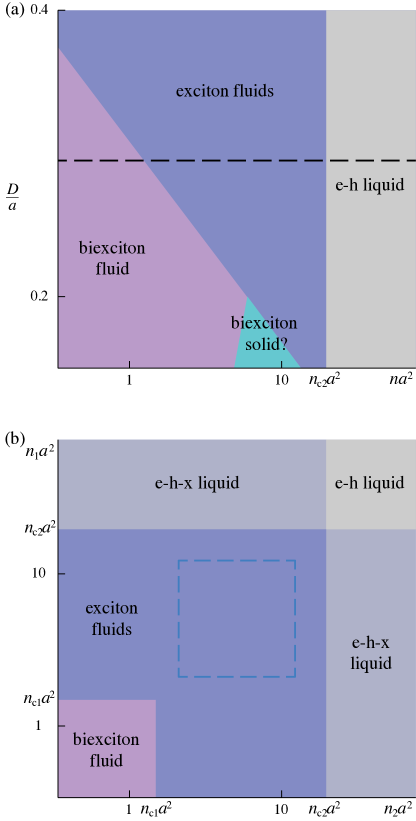
Figure 2: (a) Schematic zero-temperature phase diagram of a symmetric two-plane exciton system, $n_{1}=n_{2}\equiv n$. (b) Schematic phase diagram for arbitrary exciton densities $n_{1}$, $n_{2}$. The interplane distance $D$ is fixed at the position of the dashed line in panel (a); “e”, “h”, and “x” stand for electron, hole, and exciton, respectively. The biexciton fluid contains some unpaired excitons if $n_{1}\neq n_{2}$. The dashed square indicates the $n_{1}$–$n_{2}$ range plotted in Fig. 4.

The remainder of this article is organized as follows. In Sec. II, we define the model we study. In Sec. IV, we report the ground-state energies and sound velocities calculated for relatively high exciton densities. We verify the accuracy of our HNC method by comparing it with the available Monte-Carlo simulations for the single-plane problem. In Sec. V, we qualitatively discuss the low-density paired phase. In Sec. VI, we study the regime where only one of the planes is dilute. Here the analysis can be made more quantitative using the analogy to the polaron problem. We compute the energies and effective masses of such exciton-polarons. We give concluding remarks in Sec. VII. Additional calculations and technical details are presented in the Appendix.

II Model

Our model is sketched in the inset of Fig. 1. The white strips indicate the tunneling barrier regions, which are classically forbidden for the carriers. The dark strips represent the layers populated alternatively by electrons ($-$) and holes ($+$). We assume that all the electrons and holes are paired into excitons and that the pairing occurs only in the two top and two bottom layers that have center-to-center separations $d_{1}$ and $d_{2}$, respectively. We ignore the possibility of exciton formation by binding carriers from the two middle layers. This should be legitimate if the corresponding interlayer distance $D-(d_{1}+d_{2})/2$ is sufficiently large. We also ignore any internal dynamics of excitons, which allows us to treat the quadrilayer as two coupled planes of excitons. Here, as in Sec. I, the term “layer” pertains to electrons and holes, while “plane” describes a 2D sheet of excitons. Specifically, the exciton plane $\alpha=1$ ($2$) represents the two top (two bottom) layers seen as a unit. The effective Hamiltonian we study is the sum of the kinetic and interaction energies:

$$H =H_{1}+H_{2}+H_{12}\,,$$ (1)

$$H_{\alpha} =-\frac{\hbar^{2}}{2m}\sum_{i=1}^{N_{\alpha}}\nabla^{2}_{i}+\sum_{i<j}u_{\alpha\alpha}\left(\mathbf{r}^{i}_{\alpha}-\mathbf{r}^{j}_{\alpha}\right),$$ (2)

$$H_{12} =\sum_{i=1}^{N_{1}}\sum_{j=1}^{N_{2}}u_{12}\left(\mathbf{r}^{i}_{1}-\mathbf{r}^{j}_{2}\right).$$ (3)

Here $\mathbf{r}^{i}_{\alpha}$’s are the exciton coordinates, $N_{\alpha}$ is their number, and $n_{\alpha}=N_{\alpha}/\Omega$ is their density in plane $\alpha$; $\Omega$ is the system area. We assume that the effective mass $m$ of the excitons is the same in the two planes (approximately $0.20$ of the bare electron mass in $\rm{GaAs}/{\rm{Ga}}{\rm{Al}}{\rm{As}}$ nanostructures Choksy et al. (2021)).

In order to model the effective interaction potentials $u_{\alpha\beta}(r)$ we need to know the charge distribution of the exciton. In principle, it can be determined by solving the two-body e-h binding problem numerically. However, the result depends on many microscopic details, such as the thickness of the layers, the electric field, and the properties of the tunneling barriers Szymanska and Littlewood (2003); Sivalertporn et al. (2012). As a simpler alternative, we assume that the charge density distribution of every electron (hole) in a given layer $j$ is an isotropic Gaussian:

$$|\psi(r,z)|^{2}\propto\exp\left[-\frac{(z-z_{j})^{2}+r^{2}}{2c^{2}}\right]\,.$$ (4)

Here $r$ is the in-plane distance of the particle from the center of the exciton and $z$ is its out-of-plane coordinate, with $z_{j}$ being the midpoint $z$-coordinate of layer $j$. The Coulomb interaction energy of two such Gaussians of charge $e_{0}$ each has the following analytic form

$$v(r,z)=\frac{e_{0}^{2}}{\kappa\sqrt{r^{2}+z^{2}}}\,{\rm{erf}}\left(\frac{\sqrt{r^{2}+z^{2}}}{2c}\right),$$ (5)

which is familiar from the Ewald summation method. The second factor in Eq. (5), containing the error function $\mathrm{erf}(x)$, smooths out the short-range divergence of the Coulomb potential. Later we will need the 2D Fourier transform of $v(r,z)$ with respect to $r$, which is given by

$$\tilde{v}(k,z) \equiv\int v(r,z)e^{-i\mathbf{k}\cdot\mathbf{r}}d^{2}r$$ (6)

$$=\frac{e_{0}^{2}}{\kappa}\,\frac{\pi}{k}\sum_{\sigma=\pm 1}e^{k^{2}c^{2}+\sigma kz}{\rm{erfc}}\left(kc+\frac{\sigma z}{2c}\right),$$ (7)

where $k=|\mathbf{k}|$ and $\mathrm{erfc}(x)=1-\mathrm{erf}(x)$.

In our approximate model the charge density distribution of the exciton consists of two oppositely-charged Gaussians [Eq. (4)] aligned in-plane. Accordingly, the interplane $u_{12}(r)$ and intraplane $u_{\alpha\alpha}(r)$ exciton interaction potentials are given by

$$u_{12}(r) =v\left(r,D+\frac{d_{1}-d_{2}}{2}\right)+v\left(r,D-\frac{d_{1}-d_{2}}{2}\right)$$

$$-v\left(r,D+\frac{d_{1}+d_{2}}{2}\right)-v\left(r,D-\frac{d_{1}+d_{2}}{2}\right),$$ (8)

$$u_{\alpha\alpha}(r) =2v\left(r,0\right)-2v\left(r,d_{\alpha}\right).$$ (9)

These potentials are plotted in Fig. 1 for representative parameter values Choksy et al. (2021). In this example, $u_{11}(r)$ and $u_{22}(r)$ are always positive while $u_{12}(r)$ is negative at $r<57\,\mathrm{nm}$, see also Fig. 7(d) below. All the potentials decay as $u_{\alpha\beta}(r)\propto r^{-3}$ at large $r$, which classifies them as short-range interactions. The width $c$ of the Gaussian in Eq. (4) affects mainly the short-distance behavior of the intraplane potentials $u_{\alpha\alpha}(r)$. Since the excitons in the same plane strongly avoid each other (Sec. IV), this adjustable parameter has only a minor influence on the many-body properties. The properties of our main interest are the ground-state energy and the low-energy excitation spectrum. In the following Section we discuss methods we employ to study them.

III HNC formalism

The primary many-body quantities we were able to compute include the pair correlation functions (PCFs) $g_{\alpha\beta}(r)$, the structure factors $S_{\alpha\beta}(k)$, and the energy density per unit area $e=e(n_{1},n_{2})$. The PCF is defined by

$$g_{\alpha\beta}(r)=\frac{\Omega}{N_{\alpha}N_{\beta}}\sum_{i=1}^{N_{\alpha}}\sum_{j=1}^{N_{\beta}}\left\langle\delta\left(\mathbf{r}^{i}_{\alpha}-\mathbf{r}^{j}_{\beta}-\mathbf{r}\right)\right\rangle-\frac{\delta_{\alpha\beta}}{n_{\alpha}}\delta\left(\mathbf{r}\right).$$ (10)

The structure factor is $S_{\alpha\beta}(k)=\delta_{\alpha\beta}+\sqrt{n_{\alpha}n_{\beta}}\,\tilde{h}_{\alpha\beta}(k)$ where $h_{\alpha\beta}(r)\equiv g_{\alpha\beta}(r)-1$. The tilde in $\tilde{h}_{\alpha\beta}$ denotes the 2D Fourier transform, as in Eq. (6).

The energy density can be expressed in terms of the PCF. The simplest result is obtained within the mean-field approximation, $g_{\alpha\beta}=1$, $S_{\alpha\beta}=\delta_{\alpha\beta}$ that neglects correlations. This mean-field energy density is

$$e_{\mathrm{mf}}(n_{1},n_{2})=\frac{1}{2}\sum_{\alpha\beta}\tilde{u}_{\alpha\beta}(0)n_{\alpha}n_{\beta}\,.$$ (11)

For our model interaction potentials, we find

$$\tilde{u}_{\alpha\alpha}(0) =\int u_{\alpha\alpha}(r)d^{2}r=2\lim_{q\to 0}[\tilde{v}(q,0)-\tilde{v}(q,d_{\alpha})]$$ (12)

$$=\frac{4\pi e_{0}^{2}}{\kappa}\left[d_{\alpha}\,\mathrm{erf}\left(\frac{d_{\alpha}}{2c}\right)-\frac{2c}{\sqrt{\pi}}\left(1-e^{-\frac{d_{\alpha}^{2}}{4c^{2}}}\right)\right],$$ (13)

so that in the zero-thickness limit, $c\to 0$, we get

$$\tilde{u}_{\alpha\alpha}(0)\to\frac{4\pi e_{0}^{2}}{\kappa}\,d_{\alpha}\,,\qquad\tilde{u}_{12}(0)\to 0\,.$$ (14)

This simplified expression yields the “capacitor formula”

$$e_{\mathrm{cap}}(n_{1},n_{2})=\frac{2\pi e_{0}^{2}}{\kappa}\,\left(n_{1}^{2}d_{1}+n_{2}^{2}d_{2}\right),$$ (15)

which is so named because it resembles the total energy of two parallel-plate capacitors of dielectric thickness $d_{1}$ and $d_{2}$. There is no $n_{1}n_{2}$ term in this quadratic form since such parallel-plate capacitors do not produce external electric field, and so do not interact. Equation (15) implies that any appreciable effect of interplane interactions can arise only from correlations.

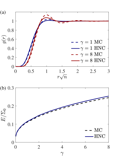
Figure 3: Comparison of our HNC calculations with prior Monte-Carlo results Astrakharchik et al. (2007, 2008); Büchler et al. (2007) for a model system of single-plane dipolar bosons. (a) PCF computed for two values of $\gamma=na^{2}$ representative of correlated exciton liquids in ${\rm{GaAs}}$ Choksy et al. (2021). Note that the liquid-solid transition occurs at $\gamma\approx 300$. (b) Energy per particle $E$ in units of the capacitor self-energy $\Sigma_{0}$ (see text) as a function of $\gamma$ for fixed $d=6a_{x}$.

To go beyond the mean-field theory we employed the zero-temperature HNC (more precisely, HNC/$0$) method for multi-species systems Chakraborty (1982a, b). In this method, the ground-state wavefunction $\Psi$ is assumed to be in the Jastrow-Feenberg product form:

$$\Psi=\prod_{\alpha=1,2}\,\prod_{i<j}f_{\alpha}\left(\mathbf{r}^{i}_{\alpha}-\mathbf{r}^{j}_{\alpha}\right)\prod_{i,\,j}f_{12}\left(\mathbf{r}^{i}_{1}-\mathbf{r}^{j}_{2}\right).$$ (16)

Functions $f_{1}$, $f_{2}$, $f_{12}$ obey a set of nonlinear equations

$$\left(-\frac{\hbar^{2}}{m}\nabla^{2}+u_{\alpha\beta}(r)+w_{\alpha\beta}(r)\right)\sqrt{g_{\alpha\beta}(r)}=0\,,$$ (17)

where the so-called induced potentials $w_{\alpha\beta}(r)$ are defined via their Fourier transforms

$$\tilde{w}_{\alpha\beta}(k)=\frac{\epsilon(k)}{2\sqrt{n_{\alpha}n_{\beta}}}\left[3\mathrm{I}-2\mathrm{S}-(\mathrm{S}^{-1})^{2}\right]_{\alpha\beta},$$ (18)

$\mathrm{S}$ is the $2\times 2$ matrix made of $S_{\alpha\beta}(k)$, $\mathrm{I}$ is the identity matrix, and

$$\epsilon(k)=\frac{\hbar^{2}k^{2}}{2m}$$ (19)

is the bare single-particle energy. These equations can be solved numerically by iterations Chakraborty (1982a, b). The energy density of the system is then calculated from Chakraborty (1982b)

$$e =\frac{1}{2}\int d^{2}r\sum_{\alpha\beta}n_{\alpha}n_{\beta}\left[g_{\alpha\beta}u_{\alpha\beta}+\frac{\hbar^{2}}{m}(\nabla\sqrt{g_{\alpha\beta}})^{2}\right]$$ (20)

$$-\frac{1}{4}\int\frac{d^{2}k}{(2\pi)^{2}}\epsilon(k)\,\mathrm{tr}\left(3\mathrm{I}-3\mathrm{S}+\mathrm{S}^{2}-\mathrm{S}^{-1}\right).$$ (21)

The performance of the HNC method has been previously shown to be very good Abedinpour et al. (2012) in a single-plane system, $N_{1}=0$. The corresponding ground-state wavefunction is obtained from Eq. (16) by dropping $f_{1}$ and $f_{12}$ terms while in the HNC equations one needs to set $S_{11}=1$, $S_{12}=0$, and solve for $g_{22}$ only. To simplify notations, we also drop the subscripts in $n_{2}$, $S_{22}$, $g_{22}$, etc. In this calculation the point-dipole limit $u(r)=e_{0}^{2}d^{2}/r^{3}$ was used for which Monte-Carlo results are available Astrakharchik et al. (2007, 2008); Büchler et al. (2007). Such a system can be characterized by the dimensionless interaction strength $\gamma=na^{2}$, where $a=d^{2}/a_{x}$ is the dipole length introduced in Sec. I. Note that $\gamma\sim 4$ for density $n\sim 1.0\times 10^{10}\,\mathrm{cm}^{-2}$ and dipole length $a\sim 200\,\mathrm{nm}$ typical of ${\rm{GaAs}}$ devices. We repeated this benchmark calculation on a denser grid of density points in the practical range $\gamma<8$ of moderately strong interactions. In Fig. 3 we present the results for the PCF and the energy per particle $E=e(n)/n$ in units of the “capacitor self-energy” $\Sigma_{0}=({4\pi e_{0}^{2}}/{\kappa})({nd})$. From Fig. 3, we can see that the HNC and the more accurate Monte-Carlo methods are indeed in a good agreement. Both methods predict that the particles strongly avoid each other at distances shorter than the average intraplane spacing $n^{-1/2}$, which enables them to reduce the system energy significantly below the mean-field value.

IV High to moderate exciton densities

Let us turn to our main subject, the two-plane exciton system. Including all three correlation factors $f_{1}$, $f_{2}$, $f_{12}$, and solving the HNC equations for a range of densities $n_{1},n_{2}$, we arrived at the results presented in Fig. 4. The geometrical and physical parameters used in the calculations are specified in the caption of Fig. 1. Qualitatively, the behavior of the obtained energy density $e(n_{1},n_{2})$ resembles the predictions of the mean-field theory. However, the energy density is greatly reduced compared to Eq. (15) and this reduction is stronger at small $n_{1}$, $n_{2}$, as in the single-plane test case, Fig. 3(b). The effect of many-body correlations can be seen more clearly in derivatives of function $e(n_{1},n_{2})$, which are also more directly connected to quantities measured in experiments. For example, the first derivatives, i.e., the chemical potentials

$$\Sigma_{\alpha}=\frac{\partial e}{\partial n_{\alpha}},\qquad\alpha=1,2,$$ (22)

are related to the exciton photoluminescence energies. Calculations of $\Sigma_{\alpha}$ and their comparison with experiments in ${\rm{GaAs}}$ systems have been reported in Ref. Choksy et al. (2021). Here we focus on the second derivatives $\partial^{2}e/\partial n_{\alpha}\partial n_{\beta}$ of the energy density, which determine another physical observable: the spectrum of low-energy excitations.

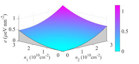
Figure 4: Energy density given by the HNC.

Recall that the elementary excitations of a single-component Bose liquid with short-range interactions are phonons with a linear dispersion at small momentum: $E(k)\simeq\hbar vk$. Our two-plane system supports two phonon modes that represent coupled oscillations of the exciton densities. Their velocities $v_{j}$, where $j=1,2$, satisfy the condition that $mv_{j}^{2}$ are the eigenvalues of a $2\times 2$ matrix with elements

$$\sqrt{n_{\alpha}n_{\beta}}\,\frac{\partial^{2}e}{\partial n_{\alpha}\partial n_{\beta}}\,.$$ (23)

We define $v_{2}$ ($v_{1}$) to be the larger (smaller) of the two velocities.

Within the mean-field theory, the second derivatives in question are equal to the plane-integrated interaction potentials, e.g.,

$$\frac{\partial^{2}e_{\mathrm{mf}}}{\partial n_{1}\partial n_{2}}=\tilde{u}_{12}(0)\,.$$ (24)

Since $\tilde{u}_{12}(0)$ is small, the mean-field theory predicts that the two phonon modes are nearly decoupled. The HNC method should give a superior approximation for the energy density, and thus for the coupling (“mode repulsion”) of the sound velocities. In Fig. 5(a, b) we plotted $v_{1}$ and $v_{2}$ deduced from the HNC for the same parameters as in Figs. 1 and 4. The typical magnitude of the sound velocities is a few times $10^{6}\,\mathrm{cm/s}$. For reference, the kinetic energy of a free exciton with such a velocity is of the order of several degrees $\mathrm{K}$. Figure 5(b) shows that as $n_{1}$ increases at fixed $n_{2}$, the dependence of $v_{2}$ on $n_{1}$ flattens out. Similar trend is observed when $n_{2}$ increases at fixed $n_{1}$. This occurs because the interplane correlations weaken at large densities. To reveal the mode coupling we plotted the difference $\Delta v=v_{2}-v_{1}$ in Fig. 5(c). The mode repulsion is evidenced by the appreciable value of $\Delta v$ at the bottom of the deep trough running roughly diagonally through this plot.

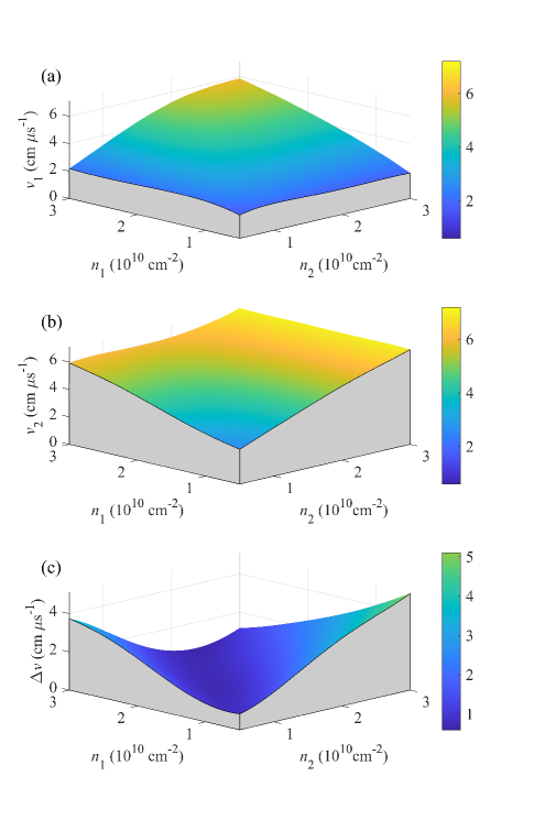
Figure 5: Sound velocities as functions of the exciton densities. (a) $v_{1}$, the slower velocity (b) $v_{2}$, the faster velocity (c) $\Delta v=v_{2}-v_{1}$, the difference of the two.

The full momentum dependence of particle density excitation spectra $E_{j}(k)$ can reveal further information about correlations. The mean-field (Gross-Pitaevskii) theory predicts

$$\begin{split}E_{\mathrm{mf}}^{2}(k)&=\epsilon^{2}(k)+\epsilon(k)(n_{1}\tilde{u}_{11}+n_{2}\tilde{u}_{22})\\ &\pm\epsilon(k)\sqrt{(n_{1}\tilde{u}_{11}-n_{2}\tilde{u}_{22})^{2}+4n_{1}n_{2}\tilde{u}^{2}_{12}}\,.\end{split}$$ (25)

On the other hand, the exact $E_{j}(k)$ are determined by the poles of the dynamic structure factor (more generaly, by the regions of the $k$–$E$ space where this factor has a nonzero imaginary part). Unfortunately, the dynamical structure factor is not available from the HNC. Following previous work Astrakharchik et al. (2008); Hufnagl et al. (2011); Macia et al. (2012); Abedinpour et al. (2012) we estimate $E_{j}(k)$ from the static structure factors $S_{\alpha\beta}(k)$ using the Bijl-Feynman approximation (BFA) Mahan (2013).

The BFA can be derived by diagonalizing the Hamiltonian in a subspace of density-wave states

$$|\mathbf{k}_{\alpha}\rangle\equiv\frac{1}{\sqrt{N_{\alpha}^{\phantom{\dagger}}}}|\rho^{\dagger}_{\alpha}(\mathbf{k})|0\rangle,$$ (26)

where $\rho_{\alpha}(\mathbf{k})=\sum_{j=1}^{N_{\alpha}}e^{-i\mathbf{k}\cdot\mathbf{r}_{\alpha}^{j}}$ is the density operator in plane $\alpha$. The key to the derivation are the following identities Mahan (2013)

$$\langle\mathbf{k}_{\alpha}|\mathbf{k}_{\beta}\rangle=S_{\alpha\beta}(k)+\sqrt{N_{\alpha}N_{\beta}}\,\delta_{\mathbf{k}=0},$$ (27)

$$\langle\mathbf{k}_{\alpha}|H^{\prime}|\mathbf{k}_{\beta}\rangle=\delta_{\alpha\beta}S_{\alpha\alpha}(k)\epsilon(k),$$ (28)

where $H^{\prime}=H-e\Omega$ is the Hamiltonian with the ground-state energy subtracted. Using these relations, one can obtain and easily solve a $2\times 2$ matrix eigenvalue problem. The result is

$$E_{1,2}(k)=\frac{2\epsilon(k)}{S_{11}+S_{22}\mp\sqrt{(S_{11}-S_{22})^{2}+4S_{12}^{2}}}$$ (29)

and a representative BFA spectrum is shown in Fig. 6(a). This Figure demonstrates that the dispersion of the two modes remains accurately linear up to $k\sim 1/\sqrt{n_{j}}$. At larger $k$ the deviations from the linearity start to be noticeable. The dispersions subsequently develop plateau-like structures indicative of strong short-range correlations in the system. At still larger $k$, the two modes merge together, as they both approach the free-particle limit $E_{j}(k)\to\epsilon(k)$. Note that the BFA is somewhat misleading because the exact excitation spectrum at finite $k$ is not confined to two dispersion lines of infinitesimal width. It is known that the excitations span instead a continuum of energies and the BFA shows only the center-of-gravity (the first moment) of this continuum.

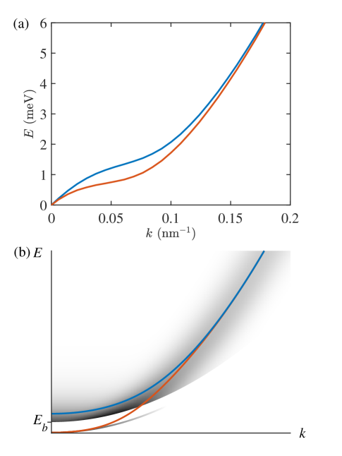
Figure 6: Collective mode spectra. (a) Mode dispersions for $n_{1}=n_{2}=2.0\times 10^{10}\,\mathrm{cm}^{-2}$ computed using the BFA. (b) A simplified sketch of the excitation spectrum in the biexciton phase. The grayscale shading represents the true spectral weight and the solid lines indicate the BFA.

V Low-density paired phase

At low densities our HNC simulations were hindered by the lack of convergence. We attribute this to the proximity of the paired superfluid phase, see Sec. I, which our standard implementation of the HNC does not describe. Hence, we can offer only a qualitative analysis of the paired phase. We focus on the symmetric case, $n_{1}=n_{2}\equiv n$, where all the excitons should pair up into biexcitons. The biexciton is a bosonic quasiparticle with the effective mass $2m$ and a certain binding energy $E_{b}$ to be discussed below. For simplicity, we suppose that no other bound exciton states exist. At energies much smaller than $E_{b}$, the system can be modeled as a single-component Bose liquid with the repulsive interaction potential

$$u_{b}(r)=u_{1}(r)+u_{2}(r)+2u_{12}(r)\,.$$ (30)

Therefore, the lowest energy excitation mode $E_{1}(k)$ is again acoustic. As $k$ increases, the dispersion of $E_{1}(k)$ should change from linear to the parabolic law for mass-$2m$ particles: $E_{1}(k)\simeq\hbar^{2}k^{2}/4m=\epsilon(k)/2$. We expect this excitation branch to gradually loose spectral weight as $k$ increases, as showed schematically by diminishing shading in Fig. 6(b). The mode should become essentially extinct at $E_{1}(k)>E_{b}$. The spectral weight gets transferred from this mode to the aforementioned excitation continuum. The boundary of the continuum

$$E(k)=E_{b}+\frac{\hbar^{2}k^{2}}{4m}$$ (31)

can be viewed as a Higgs-like mode predicted to exist in superconductors Littlewood and Varma (1982) and electron-hole bilayers Xue et al. (2020). The gap in the spectrum is the hallmark of the paired phase.

We used two methods to compute the important energy scale $E_{b}$. First, we treated the biexciton as a bound state of a pair of rigid excitons confined to two separate planes. This problem amounts to solving for the ground state of a single particle of reduced mass $\mu=m/2$ in a potential $u_{12}(r)$ where $r$ is the distance between the excitons forming the pair. For the parameters used throughout this article, we found

$$E_{b}=0.286\,\mathrm{meV}.$$ (32)

The structure of the biexciton within this approximation is described by wavefunction $\psi_{0}(r)$ shown in Fig. 7(d).

The second, more rigorous approach was to solve for the ground state of four particles, two electrons and two holes, in a quadrilayer. For this task we adopted a stochastic variational method (SVM) previously shown to be highly accurate for such few-body problems Meyertholen and Fogler (2008). The SVM result $E_{b}=0.345\,\mathrm{meV}$ was only $20\%$ larger than that of the simplified first method. [For simplicity, the SVM calculation was done in the limit $c\to 0$ in Eq. (4).]

The existence of gapped mode can also be deduced from the BFA. Indeed, let $S_{b}(k)=1+n\,\tilde{h}_{b}(k)$ be the structure factor and $g_{b}(r)=1+h_{b}(r)$ be the PCF of “rigid” biexcitons, i.e., the single-species bosonic system with the interaction potential $u_{b}(r)$ [Eq. (30)]. The intraplane structure factors and PCFs of our biexciton superfluid can then be approximated by

$$S_{\alpha\alpha}(k)=S_{b}(k)\,,\quad g_{\alpha\alpha}(r)=g_{b}(r)\,,\quad\alpha=1,2\,.$$ (33)

In turn, the interplane structure factor and PCF are

$$S_{12}(k) =S_{b}(k)+\tilde{\rho}_{0}(k)\,,$$ (34)

$$g_{12}(r) =g_{b}(r)+n^{-1}\rho_{0}(r)\,,$$ (35)

where $\rho_{0}(r)=|\psi_{0}(r)|^{2}$. At small $k$, we must have $\tilde{\rho_{0}}(k)=1-bk^{2}$ with some coefficient $b$. Equation (29) then implies a finite energy gap $E_{2}(0)=\hbar^{2}/(2mb)$. The dispersion of the two BFA branches is sketched in Fig. 6(b). The described calculation can be easily performed by the HNC. We do not show results of such calculations because the BFA does not accurately predict the true gap $E_{2}(0)=E_{b}$ and it does not describe the full distribution of the spectral weight [shading in Fig. 6(b)]. As already mentioned, the BFA determines only the first moments of the eigenmodes of the spectral weight matrix.

In the next Section we examine the case where only one plane is dilute. We show that such a regime can be studied using methods developed for the polaron problem.

VI Low density in one of the planes only

The HNC calculations become slowly converging when the exciton densities in both planes is low. However, if only one plane, say $1$, is dilute, so that $n_{1}\ll n_{2}$, then we can simplify the problem by ignoring the interactions in that plane. The implementation of HNC in such a regime has been considered to study impurities in correlated Bose liquids Chakraborty (1982b); Owen (1981); Pietiläinen and Kallio (1983). Essentially, one needs to take the $n_{1}\to 0$ limit of the full HNC equations in Sec. III. In doing so, it is convenient to redefine $S_{12}$,

$$S_{12}(k)\equiv\sqrt{N_{2}}\,S_{12}^{\mathrm{old}}(k)=n_{2}\tilde{h}_{12}(k)$$ (36)

to avoid indeterminate divide-by-zero expressions. Note that $S_{11}(k)=1$. After some algebra, the interplane “induced potential” $\tilde{w}_{12}(k)$ in Eq. (18) reduces to Chakraborty (1982b)

$$\tilde{w}_{12}(k)=-\frac{(S_{22}-1)(2S_{22}+1)}{2S_{22}^{2}}\,\frac{S_{12}}{n_{2}}\,\epsilon(k)$$ (37)

and the chemical potential $\Sigma_{1}$ to

$$\Sigma_{1}=-n_{2}\tilde{w}_{12}(0)-\frac{1}{2\Omega}\sum_{\mathbf{k}\neq 0}S_{12}(k)\tilde{w}_{12}(k)\,.$$ (38)

In the limit of high density, we can evaluate this expression analytically using the formulas

$$S_{22}(k) \simeq\frac{\epsilon(k)}{\hbar v_{2}k}\simeq\left[\frac{\epsilon(k)}{2n_{2}\tilde{u}_{22}(k)}\right]^{1/2}\ll 1\,,$$ (39)

$$S_{12}(k) \simeq-\frac{\tilde{u}_{12}(k)}{\tilde{u}_{22}(k)}\,,$$ (40)

which follow from Eqs. (25) and (29). We obtain $\tilde{w}_{12}(0)\simeq-\tilde{u}_{12}(0)$ and

$$\Sigma_{1}\simeq n_{2}\tilde{u}_{12}(0)-\frac{1}{2\Omega}\sum_{\mathbf{k}}\frac{\tilde{u}_{12}^{2}(k)}{\tilde{u}_{22}(k)}\,,\quad n_{2}\to\infty.$$ (41)

The first term, which corresponds to a weak interplane repulsion, can be recognized as the mean-field result. The second term is due to interplane correlations, which lead to an effective attraction. The linear in $n_{2}$ behavior predicted by Eq. (41) is in agreement with the numerical evaluation of Eq. (38), which we present in Fig. 7(a). Note that $\Sigma_{1}$ is negative and becomes more negative as $n_{2}$ decreases, i.e., the interplane attraction dominates over repulsion. Next, the transition to the paired phase can be estimated from the criterion $\Sigma_{1}=-E_{b}$, marked by the stars in Fig. 7(a) and (d). It occurs at $n_{2}\approx 0.5\times 10^{10}\,\mathrm{cm}^{-2}$. Although these calculations can be extended to still lower $n_{2}$, we do not trust such results, and so do not include them in the plot. The onset of the exciton pairing can also be seen from the PFC shown in Fig. 7(c). The maximum of $g_{12}(r)$ at $r=0$ can be approximated by the biexciton wavefunction squared $\psi_{0}^{2}(r)$ [Fig. 7(d)] multiplied by a coefficient that increases as $n_{2}$ decreases. At the lowest density in the plot, this coefficient is close to $n_{2}^{-1}$, which is consistent with Eq. (35).

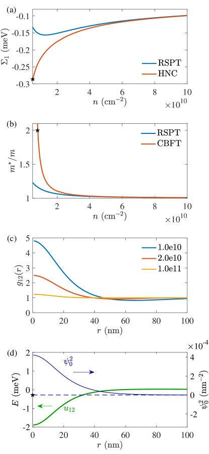
Figure 7: Parameters of a single exciton in plane $1$ interacting with a finite density plane $2$. (a) Chemical potential as a function of exciton density from the RSPT (blue) and HNC (red). (b) Effective mass from the RSPT (blue) and CBFT (red). (c) Interplane PCFs for densities indicated in the legend (in the units of $\mathrm{cm}^{-2}$). (d) The energy [dashed line, Eq. (32)] and the wavefunction squared (thin line) of a biexciton bound by the interplane interaction (solid line).

A complementary insight into the problem can be obtained by treating plane $2$ as a harmonic polarizable medium Hubert et al. (2019). In this formulation, the excitons of the low-density plane $1$ are analogous to polarons in materials with strong electron-phonon interaction Mahan (2013). Adopting the BFA for the phonon energies $E_{2}(k)$, we take the effective Hamiltonian of the higher density plane $2$ to be

$$H_{2} =\sum_{\mathbf{k}}E_{2}(k)a^{\dagger}_{\mathbf{k}}a_{\mathbf{k}}\,,$$ (42)

$$E_{2}(k) =\frac{\epsilon(k)}{S_{22}(k)}\,.$$ (43)

Here $a_{\mathbf{k}}^{\dagger}$ and $a_{\mathbf{k}}$ are the phonon creation and annihilation operators, which are related to the exciton density $\rho_{2}({\mathbf{k}})$ in plane $2$ via

$$\rho_{2}({\mathbf{k}})=\sqrt{{N_{2}}{S_{22}(k)}}\left(a_{\mathbf{k}}+a^{\dagger}_{-\mathbf{k}}\right),\quad\mathbf{k}\neq 0\,.$$ (44)

Note that Eq. (27) is satisfied. The effective Hamiltonian for a single exciton with position $\mathbf{r}$ and momentum $\mathbf{p}$ in plane $1$ has the Fröhlich form

$$H_{F}=H_{2}+\frac{p^{2}}{2m}+\frac{1}{\Omega}\sum_{\mathbf{k}\neq 0}\tilde{u}_{12}(k)e^{i\mathbf{k}\cdot\mathbf{r}}\rho_{2}({\mathbf{k}})+n_{2}\tilde{u}_{12}(0),$$ (45)

where the last term represents the $\mathbf{k}=0$ contribution.

The two commonly studied properties of a polaron are its energy shift and effective mass $m^{*}$. The former is equivalent to our chemical potential $\Sigma_{1}$ [Eq. (22)]. A simple starting point for estimating $\Sigma_{1}$ and $m^{*}$ is the Rayleigh-Schrödinger perturbation theory (RSPT) Mahan (2013). According to the RSPT, the self-energy $\Sigma(\mathbf{k})$ of the exciton in plane $1$ is

$$\Sigma(\mathbf{k})=n_{2}\tilde{u}_{12}(0)+\frac{n_{2}}{\Omega}\sum_{\mathbf{q}\neq 0}\frac{S_{22}(q)u_{12}^{2}(q)}{\epsilon(\mathbf{k})-\epsilon(\mathbf{k}-\mathbf{q})-E_{2}(q)}\,.$$ (46)

To compute $\Sigma_{1}$ and $m^{*}$ this self-energy is expanded near zero momentum to the order $O(k^{2})$:

$$\Sigma(\mathbf{k})=\Sigma_{1}-\frac{\hbar^{2}k^{2}}{2m}\eta+\ldots\,,$$ (47)

which yields

$$\Sigma_{1} =n_{2}\tilde{u}_{12}(0)-\frac{n_{2}}{\Omega}\sum_{\mathbf{k}\neq 0}\frac{\tilde{u}_{12}^{2}(k)}{\epsilon(k)}\frac{S_{22}^{2}(k)}{1+S_{22}(k)}\,,$$ (48)

$$\eta =\frac{2n_{2}}{\Omega}\sum_{\mathbf{k}\neq 0}\frac{\tilde{u}_{12}^{2}(k)}{\epsilon^{2}(k)}\,\frac{S_{22}^{4}(k)}{\left[1+S_{22}(k)\right]^{3}}\,.$$ (49)

The effective mass is given by

$$m^{*}=\frac{m}{1-\eta}\,.$$ (50)

We evaluated these expressions using the structure factor $S_{22}(k)$ supplied by the single-plane HNC and plotted the results in Fig. 7(a) and (b). Comparing them with the more reliable HNC calculations, we can conclude that RSPT can be adequate only at densities above $n_{2}\sim 2\times 10^{10}\,\mathrm{cm}^{-2}$. In that regime, the mass renormalization is still less than $10\%$, see Fig. 7(b). A possible improvement of the RSPT is the Brillouin-Wigner perturbation theory. Besides $\Sigma_{1}$ and $m^{*}$, this theory (Appendix A) also predicts some intriguing effects such as repulsive polarons. However, it is difficult to judge how reliable these predictions are.

Another polaron-theory-like approach for calculating the effective mass is the correlated basis functions perturbation theory (CBFT) Fabrocini et al. (2002). As described in Appendix B, the CBFT gives

$$\eta=\frac{1}{2n_{2}\Omega}\sum_{\mathbf{k}}\frac{S_{12}^{2}(k)}{1+S_{22}(k)}\,.$$ (51)

The corresponding $m^{*}$ as a function of $n_{2}$ is shown in Fig. 7(b). One can see that the CBFT and RSPT agree at high density. [This can also be verified using Eqs. (39) and (40).] As $n_{2}$ decreases, the two perturbation theories diverge from one another. The CBFT predicts a steep increase of the effective mass $m^{*}$ of the exciton-polaron at low $n_{2}$, see Fig. 7(b). From this plot we can infer the paired-phase boundary using the criterion $m^{*}=2m$. The corresponding density $n_{2}\approx 0.8\times 10^{10}\,\mathrm{cm}^{-2}$ [marked by the star in Fig. 7(b)] is somewhat larger than our previous estimate based on $\Sigma_{1}$ [the star in Fig. 7(a)]. We speculate that the true phase boundary may be located somewhere in between these two estimates.

VII Discussion

Our work was motivated by recent experiments with e-h-e-h quadrilayer systems Hubert et al. (2019); Choksy et al. (2021) that showed evidence for attraction of interlayer excitons. We modeled the quadrilayer as a two-plane system of excitons with competing (attractive and repulsive) dipolar interactions. Using two-species HNC formalism, we calculated several zero-temperature properties of the system, including the exciton chemical potentials, in the strongly correlated low-density regime. Our calculations predict a much weaker attraction effect compared to what was observed experimentally. Within our model, the red shift of the chemical potentials and thus the exciton photoluminescence energy cannot exceed the interplane biexciton binding energy $\sim 0.3\,\mathrm{meV}$ [Eq. (32)]. On the other hand, photoluminescence red shifts as large as several $\mathrm{meV}$ have been observed in the experiments Hubert et al. (2019); Choksy et al. (2021). Disorder effects may play some role in explaining this discrepancy. As suggested in Ref. Choksy et al., 2021, trapping by defects effectively enhances the exciton mass, which in turn increases the polaron energy shift and the biexciton binding. However, such an increase does not seem to be large enough to fully account for the discrepancy between the theory and experiment, and so further study of this problem is needed.

Another possible line of future investigation of exciton interactions and correlations is probing their collective excitations. To this end we computed the velocities of the two gapless sound modes that should exist in our system. We also discussed qualitatively how one of the modes should become gapped in the dilute limit due to the formation of interplane biexcitons. To the best of our knowledge, collective modes of exciton condensates have not yet been discovered experimentally. However, dispersing modes have been detected in (intralayer) exciton-polariton systems Utsunomiya et al. (2008); Stepanov et al. (2019); Ballarini et al. (2020) using position- and angle-resolved optical spectroscopy. Additionally, discrete collective resonances have been observed in trapped exciton-polariton liquids Estrecho et al. (2021) using time-resolved imaging. The latter technique may be well suited for excitons because of their long lifetimes, relatively slow dynamics, and one’s ability to manipulate or “shake” the traps using external electric gates High et al. (2009a, b); Kuznetsova et al. (2010). If excitons are confined in a trap of size $L$, the lowest resonant frequency should be of the order of $f\sim{v}/{2L}$ where $v$ is the mode velocity. If we take $L\sim 50\,\mu\mathrm{m}$ and $v\sim 5\times 10^{6}\,\mathrm{cm}/\mathrm{s}$ (per Sec. IV), then $f\sim 5\,\mathrm{GHz}$. The detection of such a resonant mode does not require complicated ultrafast optics. Given the detailed geometry of the trap, more accurate computations of the resonant frequencies could be done using our results for the sound velocities as an input.

Note that exciton-polaritons have a very small effective mass and interact weakly, and so they do not typically form strongly correlated liquids. In fact, the measured collective mode dispersions are only slightly different from the free-particle ones and the difference can be adequatly described by the mean-field theory [similar to Eqs. (11), (25)]. In contrast, interlayer excitons are usually strongly correlated, so that more sophisticated many-body theory is needed to study them. We hope that our work will stimulate further experimental and theoretical work on e-h and e-h-e-h exciton systems.

Appendix A Brillouin-Wigner perturbation theory

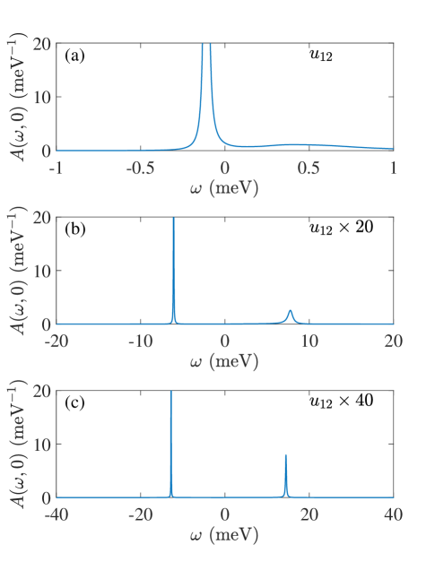
Figure 8: Spectral functions for the particles in the dilute layer for the (a) nominal (b) $10$ times enhanced, and (c) $40$ times enhanced interlayer interaction strength.

In this variant of the perturbation theory, the self-energy of the particle in plane $1$ is energy-dependent, i.e., not restricted to be on-shell:

$$\Sigma(k,E)=\frac{n_{2}}{\Omega}\sum_{\mathbf{q}}\frac{S_{22}(q)u_{12}^{2}(q)}{E-\epsilon({\mathbf{k}-\mathbf{q}})-E_{2}(q)+i\Gamma}\,,$$ (52)

where $\Gamma>0$ is a phenomenological damping parameter. The renormalized dispersion $E(k)$ of this particle is found from the maxima of the spectral function

$$A(k,E)=-2\,\mathrm{Im}\left[\frac{1}{E-\epsilon(k)-\Sigma(k,E)}\right].$$ (53)

As an example, we performed the calculation for $n_{2}=0.5\times 10^{10}\,{\mathrm{cm}^{-2}}$, $\mathbf{k}=0$, and $\Gamma=0.05\,\mathrm{meV}$. For the nominal interlayer interaction strength, we find a strong peak [Fig. 8(a)], whose location is near $\Sigma_{1}$ of the RSPT. Additionally, at higher energies there is a hint of another weak peak. The additional dispersion branch associated with this secondary peak is analogous to “repulsive polarons” in a system of excitons interacting with a Fermi sea of electrons Schmidt et al. (2012). To make the repulsive polaron more apparent, we repeated the calculation with the interaction potential $u_{12}(r)$ artificially enhanced by a factor of $20$ and $40$, see Fig. 8(b) and (c), respectively.

Appendix B Correlated basis functions perturbation theory

Let $|0\rangle$ and $|1\rangle$ be the ground states of the system containing respectively, zero and one excitons in plane $1$. The energy difference between these states is the self-energy of the exciton in plane $1$ at zero momentum, $\Sigma_{1}=\Sigma(0)$. The HNC results for $\Sigma_{1}$ have been discussed in Sec. VI. To obtain the exciton effective mass we need to know the self-energy $\Sigma(\mathbf{k})$ at finite momenta. Following previous work Fabrocini et al. (2002), we first consider a set of functions that are direct products of the density wave states in the two planes:

$$\left|\Psi_{\mathbf{k},\mathbf{q}}\right\rangle=\frac{1}{\sqrt{N_{2}^{\phantom{1}}}}e^{i(\mathbf{k}-\mathbf{q})\cdot\mathbf{r}}\rho^{\dagger}_{2}(\mathbf{q})|1\rangle,$$ (54)

We refer to the $\mathbf{q}\neq 0$ functions as the one-phonon states and the $\mathbf{q}=0$ function as the zero-phonon state. Next, we orthogonalize the former with respect to the latter:

$$|\mathbf{k},\mathbf{q}\rangle =\frac{\left|\Psi_{\mathbf{k},\mathbf{q}}\right\rangle-N_{2}^{-1}\left|\Psi_{\mathbf{k},0}\right\rangle\left\langle\Psi_{\mathbf{k},0}|\Psi_{\mathbf{k},\mathbf{q}}\right\rangle}{\mathcal{N}_{\mathbf{k},\mathbf{q}}^{1/2}},$$ (55)

$$\mathcal{N}_{\mathbf{k},\mathbf{q}} =\left\langle\Psi_{\mathbf{k},\mathbf{q}}|\Psi_{\mathbf{k},\mathbf{q}}\right\rangle-N_{2}^{-1}\left|\left\langle\Psi_{\mathbf{k},0}|\Psi_{\mathbf{k},\mathbf{q}}\right\rangle\right|^{2},$$ (56)

where $N_{2}=\left\langle\Psi_{\mathbf{k},0}|\Psi_{\mathbf{k},0}\right\rangle$ and $\mathcal{N}_{\mathbf{k},\mathbf{q}}$ are the normalization factors. Note that

$$\left\langle\Psi_{\mathbf{k},\mathbf{q}}|\Psi_{\mathbf{k},\mathbf{q}}\right\rangle =S_{22}(q)\,,$$ (57)

$$\left\langle\Psi_{\mathbf{k},0}|\Psi_{\mathbf{k},\mathbf{q}}\right\rangle =S_{12}(q)\,.$$ (58)

Ignoring the terms of order $O(N_{2}^{-1})$, the matrix elements of the Hamiltonian in this basis are

$$\langle\mathbf{k},\mathbf{q}|H^{\prime}|\mathbf{k},\mathbf{q}\rangle =\epsilon(\mathbf{k}-\mathbf{q})+E_{2}(q)\,,$$ (59)

$$\langle\mathbf{k},0|H^{\prime}|\mathbf{k},\mathbf{q}\rangle =-\frac{S_{12}(q)}{\sqrt{N_{2}S_{22}(q)}}\,\frac{\hbar^{2}}{2m}\,(\mathbf{k}\cdot\mathbf{q}).$$ (60)

The orthogonalization of the basis is important to get Eq. (60). The lowest-order perturbative correction to the energy of $\left|\Psi_{\mathbf{k},0}\right\rangle$ state is

$$\Sigma(\mathbf{k})-\Sigma_{1}=\sum_{\mathbf{q}\neq 0}\frac{|\langle\mathbf{k},0|H^{\prime}|\mathbf{k},\mathbf{q}\rangle|^{2}}{\epsilon(\mathbf{k})-\langle\mathbf{k},\mathbf{q}|H^{\prime}|\mathbf{k},\mathbf{q}\rangle}\,.$$ (61)

Expanding this expression to the order $O(k^{2})$, as in Eq. (47), we recover Eq. (51) for the mass renormalization parameter $\eta$. The CBFT can also be done Fabrocini et al. (2002) Brillouin-Wigner style by replacing $\epsilon(\mathbf{k})$ with $E$ in Eq. (61) but we have not explored that.

References

- Lozovik and Yudson (1976) Y. E. Lozovik and V. I. Yudson, Journal of Experimental and Theoretical Physics 44, 389 (1976), URL http://jetp.ac.ru/cgi-bin/dn/e_044_02_0389.pdf.
- Butov et al. (2001) L. V. Butov, A. L. Ivanov, A. Imamoglu, P. B. Littlewood, A. A. Shashkin, V. T. Dolgopolov, K. L. Campman, and A. C. Gossard, Physical Review Letters 86, 5608 (2001).
- Dorow et al. (2018) C. J. Dorow, M. W. Hasling, D. J. Choksy, J. R. Leonard, L. V. Butov, K. W. West, and L. N. Pfeiffer, Applied Physics Letters 113, 212102 (2018).
- Hagn et al. (1995) M. Hagn, A. Zrenner, G. Böhm, and G. Weimann, Applied Physics Letters 67, 232 (1995).
- Gärtner et al. (2006) A. Gärtner, A. W. Holleitner, J. P. Kotthaus, and D. Schuh, Applied Physics Letters 89, 052108 (2006).
- Hammack et al. (2009) A. T. Hammack, L. V. Butov, J. Wilkes, L. Mouchliadis, E. A. Muljarov, A. L. Ivanov, and A. C. Gossard, Physical Review B 80, 155331 (2009).
- Leonard et al. (2009) J. R. Leonard, Y. Y. Kuznetsova, S. Yang, L. V. Butov, T. Ostatnicky, A. Kavokin, and A. C. Gossard, Nano Letters 9, 4204 (2009).
- Lazić et al. (2010) S. Lazić, P. V. Santos, and R. Hey, Physica E: Low-dimensional Systems and Nanostructures 42, 2640 (2010), URL http://www.sciencedirect.com/science/article/pii/S1386947709004238.
- Alloing et al. (2012) M. Alloing, A. Lemaître, E. Galopin, and F. Dubin, Physical Review B 85, 245106 (2012), URL https://doi.org/10.1103/PhysRevB.85.245106.
- Lazić et al. (2014) S. Lazić, A. Violante, K. Cohen, R. Hey, R. Rapaport, and P. V. Santos, Physical Review B 89, 085313 (2014), URL https://doi.org/10.1103/PhysRevB.89.085313.
- Finkelstein et al. (2017) R. Finkelstein, K. Cohen, B. Jouault, K. West, L. N. Pfeiffer, M. Vladimirova, and R. Rapaport, Physical Review B 96, 085404 (2017), URL https://doi.org/10.1103/PhysRevB.96.085404.
- Hubert et al. (2019) C. Hubert, Y. Baruchi, Y. Mazuz-Harpaz, K. Cohen, K. Biermann, M. Lemeshko, K. West, L. Pfeiffer, R. Rapaport, and P. Santos, Physical Review X 9, 021026 (2019), URL https://doi.org/10.1103/PhysRevX.9.021026.
- Choksy et al. (2021) D. J. Choksy, C. Xu, M. M. Fogler, L. V. Butov, J. Norman, and A. C. Gossard, Physical Review B 103, 045126 (2021), URL https://doi.org/10.1103/PhysRevB.103.045126.
- De Palo et al. (2002) S. De Palo, F. Rapisarda, and G. Senatore, Physical review letters 88, 206401 (2002), URL https://doi.org/10.1103/PhysRevLett.88.206401.
- Tan et al. (2005) M. Y. J. Tan, N. D. Drummond, and R. J. Needs, Physical Review B 71, 033303 (2005), URL https://doi.org/10.1103/PhysRevB.71.033303.
- Lee et al. (2009) R. M. Lee, N. D. Drummond, and R. J. Needs, Phys. Rev. B 79, 125308 (2009).
- Maezono et al. (2013) R. Maezono, P. L. Ríos, T. Ogawa, and R. J. Needs, Physical review letters 110, 216407 (2013), URL https://doi.org/10.1103/PhysRevLett.110.216407.
- Astrakharchik et al. (2007) G. E. Astrakharchik, J. Boronat, I. L. Kurbakov, and Y. E. Lozovik, Phys. Rev. Lett. 98, 060405 (2007), URL https://doi.org/10.1103/PhysRevLett.98.060405.
- Astrakharchik et al. (2008) G. E. Astrakharchik, J. Boronat, J. Casulleras, I. L. Kurbakov, and Y. E. Lozovik, in Recent Progress in Many-Body Theories, edited by J. Boronat, G. E. Astrakharchik, and F. Mazzanti (World Scientific, Singapore, 2008), vol. 11 of Advances in Quantum Many-Body Theory, pp. 245–250, eprint http://arxiv.org/abs/0707.4630v1, URL https://www.worldscientific.com/doi/abs/10.1142/9789812779885_0031.
- Büchler et al. (2007) H. P. Büchler, E. Demler, M. Lukin, A. Micheli, N. Prokof’ev, G. Pupillo, and P. Zoller, Phys. Rev. Lett. 98, 060404 (2007), URL https://link.aps.org/doi/10.1103/PhysRevLett.98.060404.
- Astrakharchik et al. (2009) G. E. Astrakharchik, J. Boronat, J. Casulleras, I. L. Kurbakov, and Y. E. Lozovik, Physical Review A 79, 051602 (2009).
- Hufnagl et al. (2011) D. Hufnagl, R. Kaltseis, V. Apaja, and R. E. Zillich, Phys. Rev. Lett. 107, 065303 (2011), URL https://doi.org/10.1103/PhysRevLett.107.065303.
- Abedinpour et al. (2012) S. H. Abedinpour, R. Asgari, and M. Polini, Physical Review A 86, 043601 (2012), URL https://doi.org/10.1103/PhysRevA.86.043601.
- Mora et al. (2007) C. Mora, O. Parcollet, and X. Waintal, Phys Rev B 76, 064511 (2007).
- Bortolotti et al. (2006) D. C. E. Bortolotti, S. Ronen, J. L. Bohn, and D. Blume, Phys. Rev. Lett. 97, 160402 (2006), URL https://doi.org/10.1103/PhysRevLett.97.160402.
- Macia et al. (2012) A. Macia, D. Hufnagl, F. Mazzanti, J. Boronat, and R. E. Zillich, Phys. Rev. Lett. 109, 235307 (2012), URL https://doi.org/10.1103/PhysRevLett.109.235307.
- Macia et al. (2014a) A. Macia, J. Boronat, and F. Mazzanti, Physical Review A 90, 061601 (2014a), URL https://doi.org/10.1103/PhysRevA.90.061601.
- Macia et al. (2014b) A. Macia, G. E. Astrakharchik, F. Mazzanti, S. Giorgini, and J. Boronat, Physical Review A 90, 043623 (2014b), URL https://doi.org/10.1103/PhysRevA.90.043623.
- Filinov (2016) A. Filinov, Physical Review A 94, 013603 (2016), URL https://doi.org/10.1103/PhysRevA.94.013603.
- Cinti et al. (2017) F. Cinti, D.-W. Wang, and M. Boninsegni, Physical Review A 95, 023622 (2017), URL https://doi.org/10.1103/PhysRevA.95.023622.
- Szymanska and Littlewood (2003) M. H. Szymanska and P. B. Littlewood, Physical Review B 67, 193305 (2003), URL https://doi.org/10.1103/PhysRevB.67.193305.
- Sivalertporn et al. (2012) K. Sivalertporn, L. Mouchliadis, A. L. Ivanov, R. Philp, and E. A. Muljarov, Physical Review B 85, 045207 (2012), URL https://doi.org/10.1103/PhysRevB.85.045207.
- Chakraborty (1982a) T. Chakraborty, Physical Review B 26, 6131 (1982a), URL https://doi.org/10.1103/PhysRevB.26.6131.
- Chakraborty (1982b) T. Chakraborty, Phys. Rev. B 25, 3177 (1982b), URL https://link.aps.org/doi/10.1103/PhysRevB.25.3177.
- Mahan (2013) G. D. Mahan, Many-particle physics (Springer Science & Business Media, 2013).
- Littlewood and Varma (1982) P. B. Littlewood and C. M. Varma, Phys. Rev. B 26, 4883 (1982), URL https://link.aps.org/doi/10.1103/PhysRevB.26.4883.
- Xue et al. (2020) F. Xue, F. Wu, and A. H. MacDonald, Phys. Rev. B 102, 075136 (2020), URL https://link.aps.org/doi/10.1103/PhysRevB.102.075136.
- Meyertholen and Fogler (2008) A. D. Meyertholen and M. M. Fogler, Phys. Rev. B 78, 235307 (2008), URL https://link.aps.org/doi/10.1103/PhysRevB.78.235307.
- Owen (1981) J. C. Owen, Phys. Rev. Lett. 47, 586 (1981), URL https://doi.org/10.1103/PhysRevLett.47.586.
- Pietiläinen and Kallio (1983) P. Pietiläinen and A. Kallio, Physical Review B 27, 224 (1983), URL https://doi.org/10.1103/PhysRevB.27.224.
- Fabrocini et al. (2002) A. Fabrocini, S. Fantoni, and E. Krotscheck, Introduction to modern methods of quantum many-body theory and their applications, vol. 7 (World Scientific, 2002).
- Utsunomiya et al. (2008) S. Utsunomiya, L. Tian, G. Roumpos, C. W. Lai, N. Kumada, T. Fujisawa, M. Kuwata-Gonokami, A. Löffler, S. Höfling, A. Forchel, et al., Nature Physics 4, 700 (2008), URL https://doi.org/10.1038/nphys1034.
- Stepanov et al. (2019) P. Stepanov, I. Amelio, J.-G. Rousset, J. Bloch, A. Lemaître, A. Amo, A. Minguzzi, I. Carusotto, and M. Richard, Nature Communications 10, 3869 (2019), ISSN 2041-1723, URL https://doi.org/10.1038/s41467-019-11886-3.
- Ballarini et al. (2020) D. Ballarini, D. Caputo, G. Dagvadorj, R. Juggins, M. De Giorgi, L. Dominici, K. West, L. N. Pfeiffer, G. Gigli, M. H. Szymańska, et al., Nature Communications 11, 217 (2020), URL https://doi.org/10.1038/s41467-019-13733-x.
- Estrecho et al. (2021) E. Estrecho, M. Pieczarka, M. Wurdack, M. Steger, K. West, L. N. Pfeiffer, D. W. Snoke, A. G. Truscott, and E. A. Ostrovskaya, Phys. Rev. Lett. 126, 075301 (2021).
- High et al. (2009a) A. A. High, A. T. Hammack, L. V. Butov, L. Mouchliadis, A. L. Ivanov, M. Hanson, and A. C. Gossard, Nano Lett. 9, 2094 (2009a), URL https://doi.org/10.1021/nl900605b.
- High et al. (2009b) A. A. High, A. K. Thomas, G. Grosso, M. Remeika, A. T. Hammack, A. D. Meyertholen, M. M. Fogler, L. V. Butov, M. Hanson, and A. C. Gossard, Phys. Rev. Lett. 103, 087403 (2009b), URL https://doi.org/10.1103/PhysRevLett.103.087403.
- Kuznetsova et al. (2010) Y. Y. Kuznetsova, A. A. High, and L. V. Butov, Appl. Phys. Lett. 97, 201106 (2010), URL https://doi.org/10.1063/1.3517444.
- Schmidt et al. (2012) R. Schmidt, T. Enss, V. Pietilä, and E. Demler, Physical Review A 85, 021602 (2012), URL https://doi.org/10.1103/PhysRevA.85.021602.