The Exact WKB analysis and the Stokes phenomena of the Unruh effect and Hawking radiation

Abstract

The physical observables of quantum theory can be described by perturbation theory, which is often given by diverging power series. This divergence is connected to the existence of non-perturbative phenomena, where resurgence allows us to study this connection. Applying this idea to the WKB expansion, the exact WKB analysis gives a clear connection to non-perturbative phenomena. In this paper, we apply the exact WKB analysis to the Unruh effect and Hawking radiation. The mechanism we found in this paper is similar to the Schwinger effect of a constant electric field, where the background is static but the Stokes phenomenon appears in the temporal part. Comparing this with a sonic black hole, our calculations show a clear discrepancy between them. Then, we briefly explain how quantum backreactions can be included in the exact WKB formalism.

1 Introduction

The Stokes phenomenon is a very important phenomenon that directly explains non-perturbative particle production. It has been studied in a very broad range of applications. If special functions are used for the solutions, the Stokes phenomenon is understood as a fundamental property of the special functions. Since the Stokes phenomenon is like a fingerprint, it can be used effectively to distinguish phenomena that appear to be identical. When discussing a model in which particles are generated from a vacuum, it is very useful to focus on the Stokes phenomenon.

The Schwinger effect is a very well-known model of non-perturbative particle production and has already been studied in detail.

If one studies Hawking radiation after learning about the Schwinger effect, one will notice that many textbooks mention the similarity between the Schwinger effect and Hawking radiation. Some may be tempted to try the same analytical methods that were successful with the Schwinger effect. Some may try to figure out the difference between the Schwinger effect and the Hawking radiation by comparing their Stokes phenomena. However, such people will be puzzled there, since no article or textbook describes the Stokes phenomenon of Hawking radiation as it appears in the Schwinger effect.

Some may try to find a way by making use of Hawking’s tunneling hypothesis. This is because tunneling phenomena in quantum theory can generally be described by the Stokes phenomenon. But here, too, one encounters a strange situation. The analysis using the tunneling hypothesis is about “phenomena that do not generate the Stokes phenomena”(with the exception of some analogues, which will be described later.)

To the best of our knowledge, the Stokes phenomenon directly related to radiation near the horizon has been an unsolved problem for about half a century since Hawking’s paper. (As we will mention later in this paper, the Stokes phenomena away from the horizon are already known and has been used in the analysis of the glaybody factor and quasinormal modes.)

In this section, we will explain the above questions in some detail. Once the details of the Stokes phenomena are known, the distinction from black hole analogues will become clearer. If the Stokes phenomenon is analyzed with the Exact WKB, quantum reactions can be treated more rigorously. We will discuss these issues in the latter part of this paper.

The tunneling problem in quantum mechanics is distinct from that in classical physics. The problem is usually discussed for quantum particles that pass through a potential barrier, which is forbidden in classical mechanics. The Wentzel Kramers Brillouin Jeffreys (WKB or WKBJ) approximation, a method for finding approximate solutions to linear differential equations, is considered the most useful for this problem Berry:1972na ; Landau-Lifshitz . The WKB approximation has been applied to quantum fields propagating in curved backgrounds, such as Hawking evaporating processes Kraus:1994fj ; Parikh:1999mf ; Keski-Vakkuri:1996wom ; Srinivasan:1998ty ; Shankaranarayanan:2000qv ; Banerjee:2009wb ; Arzano:2005rs ; Akhmedova:2008dz ; Singleton:2013 ; Dumlu:2020wvd and inflationary cosmological perturbations Martin:2002vn . It has also been widely used to determine quasi-normal modes of black holes Iyer:1986np ; Konoplya:2003ii ; Konoplya:2011qq .

For a particle with energy $E$ and rest mass $m$ moves in a one-dimensional potential $V(x)$ with $E<V(x)$ in the range $a\geq x\geq b$, the amplitude of the tunneling is described by

$$e^{-\frac{1}{\hbar}\int^{b}_{a}\sqrt{2m\left(V(x)-E\right)}dx} = e^{-\frac{1}{\hbar}\int^{b}_{a}p(x)dx},$$ (1)

where $p(x)$ denotes the canonical momentum. If $V(x)$ is given by an inverted quadratic potential, exact solutions described by special functions can be obtained. It is also known that the local analysis near a turning point is well described by the Airy function Berry:1972na ; Landau-Lifshitz .

For $E>V(x)$, a similar quantum effect can be seen in the reflection, since the reflection of the particle is quantum Berry:1972na ; Landau-Lifshitz . Describing this phenomenon using Eq.(1) is a good idea in practice, but in this case, the situation is less obvious Berry:1972na . First, the turning points defined by $p(x)=0$ are not on the real axis of $x$. In the simplest case of an inverted quadratic potential, the pair of turning points appears on the imaginary axis of $x$. In this model, one can find exact solutions described by special functions (e.g., Weber functions or parabolic cylinder functions).

In more general situations, the Exact WKB(EWKB) formalism is useful. Initially, the formalism was valid only for second-order equations, but later, with the discovery of new Stokes lines NBR and virtual turning points Virtual:2015HKT , it was found to be valid for higher-order differential equations. For more mathematical details on resurgence and the EWKB formalism, see Refs.RPN:2017 ; Virtual:2015HKT ; Voros:1983 ; Delabaere:1993 ; Silverstone:2008 ; Aoki:2009 ; Takei:2008 . Using the Borel resummation, the WKB expansion is cast into a so-called Borel panel, where finite and exact results are extracted. The EWKB consists of microlocal reduction of ordinary differential operators and its application to global analysis.

In resurgence, non-perturbative effects appear from divergence. On the other hand, WKB approximation has to discard higher terms, from which the divergence appears. The EWKB helps us to understand why fine results are computed using such an approximation. Without the EWKB, it is also difficult to understand how higher terms affect the Stokes lines and their Stokes phenomena. Note that the definition of turning points is also less rigorous in the WKB approximation when compared to the EWKB; the EWKB is exact about the $\hbar$ expansion, which removes such ambiguity. In physics, the EWKB gives connection formulae, which are used to calculate the Bogoliubov coefficients of quantum particle production Kofman:1997yn ; Enomoto:2020xlf and quantum transitions in the Landau-Zener model Zener:1932ws ; Enomoto:2021hfv ; for recent applications of the EWKB, see Ref.WKB-recent:2022 .

In this paper, the Stokes phenomenon for second-order ordinary differential equations is considered in the framework of the WKB formalism. The physical observables of quantum theory can be described by perturbation theory (WKB expansion), which often gives a diverging power series. This divergence is related to the existence of non-perturbative phenomena (Stokes phenomena), so the definition of the vacuum by the WKB approximation becomes ambiguous for non-perturbative phenomena; using EWKB, definition of the vacuum becomes rigorous.

Since the Stokes phenomenon does not occur within the Stokes domain (the domain bounded by the Stokes lines), we need to find the Stokes lines where (or when) the particles are created. On the other hand, if the definition of the vacuum is independent of the observer’s differential equation, the observer may see radiation because the two sets of vacuum definitions are not identical. Both the Unruh effect Unruh:1976db and Hawking radiation Hawking:1975vcx have a static curved background, but we found the Stokes phenomenon in the temporal part. Our calculation uses the discrepancy of the vacua and the Stokes phenomenon at the same time.

Applying the EWKB to quantum scattering due to an inverted quadratic potential with $E>V(x)$, the Stokes lines is a Merged pair of Turning Points (MTP), whose exact solutions are given by the Weber function; details are described in Sec.2. The MTP structure often appears in non-perturbative analysis where a local linear approximation is valid, such as particle production in standard preheating scenarios Kofman:1997yn ; Enomoto:2020xlf and the Landau-Zener transition Zener:1932ws ; Enomoto:2021hfv . In these models, the $x$-dependence is replaced by a $t$-dependence, and local linear approximations are found in the scalar mass ($m_{\varphi}(t)\simeq vt$) of the preheating scenario and in the linear diagonal elements ($D_{\pm}(t)\simeq\pm vt$) of the Landau-Zener model Enomoto:2022nuj .

When the differential equations have poles in addition to turning points, the situation becomes less straightforward, but the Stokes phenomenon can still be described in the EWKB formalism Koike:2000 . In the space part of the WKB formalism, the Stokes lines of the Unruh effect and Hawking radiation typically take a loop structure around a pole at the horizon, where the Stokes lines do not exist in the vicinity Dumlu:2020wvd . Since there is no Stokes line near the horizon, it is not possible to see the mixing of $\pm$ solutions near the horizon (at least in the spatial part). On the other hand, for an observer standing far from the black hole, the Stokes phenomenon may appear midway between the observer and the horizon. These Stokes phenomena have been used to calculate black hole excitations and greybody factors Dumlu:2020wvd , consistent with other calculations Maldacena:1997ih . To find discrepancies between the definition of the inertial vacuum and the observer’s vacuum, global analyses are often used, in which global analytic conditions on the complex plane of the given coordinate system are examined Birrell:1982ix ; Frolov:1998wf .

Since the Unruh effect (and Hawking radiation) are intuitively local events, it seems quite natural to expect that the effects extracted from the global analysis would be encoded in the local coordinate system. An analogy with the Schwinger effect would be useful to understand the effects in the local coordinate system. It is already known Frolov:1998wf that the Unruh effect is very similar to the Schwinger effect, but the corresponding Stokes phenomenon has not been found in the Unruh effect; using the EWKB approach, we find the Stokes phenomenon in the time part of the WKB formalism of the Unruh effect. As described in Sec. 10.2 of Ref.Frolov:1998wf , a naive application of the Schwinger effect to the Unruh effect (Hawking radiation) simply replaces the field strength with the proper acceleration (surface gravity) but requires a factor of 2 ($\beta=2$ in Ref.Frolov:1998wf ). The present calculation reproduces the factor two in the Unruh effect, but no such factor is required in Hawking radiation.

To compare the WKB approximation and the EWKB, we begin with the simplest calculation of the steepest descent path method of the WKB approximation. The method of steepest descent path was first applied to cosmological particle production in Ref. Chung:1998bt and extended for higher polynomials in Ref.Enomoto:2013mla ; Enomoto:2014hza . Consider an equation of motion given by

$$\ddot{\chi}_{k}+\left[k^{2}+m_{0}^{2}-V(t)\right]\chi_{k}=0,$$ (2)

where one can choose $V(t)=-\frac{g_{2n}^{2}}{M_{*}^{2(n-1)}}(vt)^{2n}$. (Here we temporarily assume $\hbar=1$ and $c=1$.) For $n=1$, this equation coincides with the original preheating scenario of Ref.Kofman:1997yn and is similar to the scattering problem by an inverted quadratic potential. One can write down the (conventional) WKB solution given by

$$\chi_{k}=\frac{\alpha_{k}}{\sqrt{2\omega_{k}}}e^{-i\int_{-\infty}^{t}dt^{\prime}\omega_{k}(t^{\prime})}+\frac{\beta_{k}}{\sqrt{2\omega_{k}}}e^{+i\int_{-\infty}^{t}dt^{\prime}\omega_{k}(t^{\prime})},$$ (3)

where

$$\omega_{k}\equiv\sqrt{k^{2}+m_{0}^{2}-V(t)}$$ (4)

and $\alpha_{k},\beta_{k}$ have to satisfy

$$|\alpha_{k}|^{2}-|\beta_{k}|^{2}=1.$$ (5)

We consider the additional constraint (the calculation corresponds to the simplest choice of parameters in Ref.Dabrowski:2016tsx )

$$0=\dot{\left(\frac{\alpha_{k}}{\sqrt{2\omega_{k}}}\right)}e^{-i\int_{-\infty}^{t}dt^{\prime}\omega_{k}(t^{\prime})}+\dot{\left(\frac{\beta_{k}}{\sqrt{2\omega_{k}}}\right)}e^{+i\int_{-\infty}^{t}dt^{\prime}\omega_{k}(t^{\prime})}.$$ (6)

Substituting the representation (3) into (2) with the above constraint, one obtains

$$\dot{\alpha}_{k} = \beta_{k}\frac{\dot{\omega}_{k}}{2\omega_{k}}e^{+2i\int_{-\infty}^{t}dt^{\prime}\omega_{k}},$$ (7)

$$\dot{\beta}_{k} = \alpha_{k}\frac{\dot{\omega}_{k}}{2\omega_{k}}e^{-2i\int_{-\infty}^{t}dt^{\prime}\omega_{k}}.$$ (8)

Supposing that the initial state has no particle, we have

$$\alpha_{k}(-\infty)=1,\qquad\beta_{k}(-\infty)=0.$$ (9)

One can estimate the Bogoliubov coefficients for $\beta_{k}\ll 1$ by the integration given by

$$\beta_{k}(+\infty)=\int_{-\infty}^{+\infty}dt\frac{\dot{\omega}_{k}(t)}{2\omega_{k}(t)}\exp{\left[-2i\int_{-\infty}^{t}dt^{\prime}\omega_{k}(t^{\prime})\right]}.$$ (10)

This corresponds to the so-called instantaneous Hamiltonian diagonalization method Haro:2010mx . The factor $1/\omega_{k}$ at $\omega_{k}(t)=0$ of the $t$-integral is important for the calculation in Ref.Chung:1998bt . The integral in Eq.(10) can be evaluated on the complex $t$ plane using the steepest descent method. For details of the calculation, see Ref.Chung:1998bt ; Enomoto:2013mla ; Enomoto:2014hza . Although the above formulation is very simple and convenient for numerical calculations, it does not account for resurgence. In fact, although resurgence is known to link the divergence of the WKB approximation to non-perturbative phenomena, such higher-order terms are discarded from the outset in the above calculation. This discrepancy is not trivial.

The calculation of the Unruh and Hawking effects by the WKB tunneling method is expected to explain the heuristic picture of Hawking described in Ref.Hawking:1975vcx . Hawking explains the effect as a tunneling outward of positive energy modes and a tunneling inward of negative energy modes. This heuristic picture has been explored later in Ref.Kraus:1994fj ; Srinivasan:1998ty ; Parikh:1999mf ; Shankaranarayanan:2000qv ; Banerjee:2009wb ; Arzano:2005rs ; Akhmedova:2008dz ; Singleton:2013 ; Dumlu:2020wvd ; Keski-Vakkuri:1996wom , in which the action of a particle picks up an imaginary contribution when it crosses the horizon (the integral path is taken on the complex plane), and the imaginary contribution was interpreted as tunneling probability. When the static black hole is viewed in Kruskal coordinates valid on both sides of the horizon, the factor computed by “tunneling” is nothing more than a factor necessary for the WKB approximate solutions to connect smoothly inside and outside the horizon Srinivasan:1998ty ; Banerjee:2009wb , and the Stokes phenomena do not appear in the computation. In fact, since the EWKB solutions of the spatial part are in the same Stokes domain, the Stokes phenomenon does not appear by the “tunneling”.

For an analog black hole (sonic black hole), Giovanazzi Giovanazzi:2004zv found that a microscopic description of Hawking radiation explains Hawking’s original picture of tunneling. Giovanazzi’s model explains how the Stokes phenomenon can be responsible for Hawking radiation in the analog system. These analog systems are expected to gain a better understanding of Hawking radiation avoiding theoretical problems of the original black hole radiation. However, comparing the Stokes phenomena of these systems, there seems to be a crucial discrepancy between them. In Sec.2, we will show some details of the Stokes phenomena to compare the mechanisms of these models.

Sec.3 briefly describes the Stokes phenomena of Hawking radiation and a sonic black hole when quantum effects are involved, and shows why the exact definition of the $\hbar$-expansion in the EWKB is important for understanding physics beyond the semiclassical approximations.

2 The EWKB for the Stokes phenomena and Hawking radiation

The mathematical formulation of the EWKB uses $\eta\equiv\hbar^{-1}\gg 1$ for the expansion, instead of using the Planck (Dirac) constant $\hbar$. Following Ref.Voros:1983 ; Virtual:2015HKT , we start with the “Schrödinger equation” in quantum mechanics described as

$$\left[-\frac{d^{2}}{dx^{2}}+\eta^{2}Q(x)\right]\psi(x,\eta) = 0.$$ (11)

Introducing the “potential” $V(x)$ and the “energy” $E$, we define

$$Q(x) = V(x)-E.$$ (12)

Although an explicit $\eta$-dependence is not required in this section, for our later argument we write it in the following form;

$$Q(x,\eta) = \sum^{\infty}_{j=0}\eta^{-j}Q_{j}(x).$$ (13)

Writing a WKB solution as $\psi(x,\eta)=e^{R(x,\eta)}$, we have for $S(x,\eta)\equiv\partial R/\partial x$,

$$\psi = e^{\int^{x}_{x_{0}}S(x,\eta)dx},$$ (14)

where $x_{0}$ is normally taken at a turning point of the Stokes domain. For $S$, we have

$$-\left(S^{2}+\frac{\partial S}{\partial x}\right)+\eta^{2}Q = 0.$$ (15)

If one expands $S$ as $S(x,\eta)=\sum_{n=-1}^{n=\infty}\eta^{-n}S_{n}$, one will find

$$S=\eta S_{-1}(x)+S_{0}(x)+\eta^{-1}S_{1}(x)+...,$$ (16)

which leads to the following recursive relations

$$S_{-1}^{2} = Q_{0}$$ (17)

$$2S_{-1}S_{j+1} = -\left[\sum_{k=0}^{j}S_{k}S_{j-k}+\frac{dS_{j}}{dx}-Q_{j+2}\right].$$ (18)

Points of $Q_{0}(x)=0$ (which is not always identical to $Q(x,\eta)=0$) are called turning points of the equation. See Ref.Aoki:1993 for details of the calculation when $Q(x,\eta)$ depends explicitly on $\hbar=\eta^{-1}$. Later we will consider $Q(x,\hbar)$ when quantum effects are involved, but here we temporarily assume $Q(x,\eta)=Q_{0}$ . After some calculation, one will have

$$\psi = \frac{1}{\sqrt{S_{odd}}}e^{\int^{x}_{x_{0}}S_{odd}dx}$$ (20)

$$S_{odd}\equiv\sum_{j\geq 0}\eta^{1-2j}S_{2j-1}.$$

Depending on the sign of the first $S_{-1}=\pm\sqrt{Q(x)}$, there are two solutions $\psi_{\pm}$, which are given by

$$\psi_{\pm} = \frac{1}{\sqrt{S_{odd}}}\exp\left(\pm\int^{x}_{x_{0}}S_{odd}dx\right)$$ (21)

$$= e^{\pm\eta\int\sqrt{Q}dx}\sum^{\infty}_{n=0}\eta^{-n-1/2}\psi_{\pm,n}(x).$$

The above WKB expansion is usually divergent but is Borel-summable. The Borel transform is taken as

$$\psi_{\pm}^{B} = \sum^{\infty}_{n=0}\frac{\psi_{\pm,n}(x)}{\Gamma(n+\frac{1}{2})}\left(y\pm s(x)\right)^{n-\frac{1}{2}}.$$ (22)

Theorems and proofs of the EWKB are mostly given on the “Borel panel” using $\psi^{B}_{\pm}$. For physics, what is important here is the shift of the integral of the inverse-Laplace integration. The shift is determined by $S_{-1}$ as

$$\psi_{\pm} \rightarrow \Psi_{\pm}\equiv\int^{\infty}_{\mp s(x)}e^{-y\eta}\psi_{\pm}^{B}(x,y)dy,$$ (24)

$$s(x)\equiv\int^{x}_{x_{0}}S_{-1}(x)dx,$$

where the $y$-integral is parallel to the real axis. The Stokes lines are defined as the solutions of $\mathrm{Im}[s(x)]=0$. In the EWKB, the Stokes lines are exact with respect to the $\hbar$ expansion, and they are computed from first-order terms. This is a striking result given that the Stokes lines determine the intrinsic properties of quantum systems; without the EWKB, it is difficult (or impossible) to prove that the Stokes lines are unaffected by higher order terms(e.g, $S_{0},S_{1},...$). (We are not showing proofs here. See RPN:2017 ; Delabaere:1993 ; Virtual:2015HKT for more details.) Such higher-order terms are often used to avoid discontinuities in the Stokes phenomena in semiclassical approximation Dabrowski:2016tsx , but as long as the WKB approximation is used, the dilemma was that the inclusion of such terms could easily change the structure of the Stokes lines. The Exact WKB removes the notorious uncertainty of the WKB approximation and redefines the semiclassical calculation.

In typical cases, the Stokes lines are often degenerate. In such cases, a gap may appear at $\mathrm{Im}[\eta]=0$ (between $\mathrm{Im}[\eta]>0$ and $\mathrm{Im}[\eta]<0$). This gap has already been resolved analytically by the normalization factor (called Voros coefficient Voros:1983 ), whose analytic calculation is given in Ref.Voros:1983 ; Silverstone:2008 ; Takei:2008 ; Aoki:2009 for MTP (Merged pair of simple Turning Points) and a loop structure of a Bessel-like equation Aoki:2019 . More simply, the normalization coefficient can be computed using a simple consistency relation Berry:1972na , but that method cannot determine the phase of the coefficient.

To explicitly show the calculation of the connection matrix using the EWKB, we begin with

$$\frac{d^{2}\psi}{dt^{2}}+\eta^{2}\left[E+g^{2}_{2}v^{2}t^{2}\right]\psi=0.$$ (25)

For $E<0$, turning points will appear on the real axis. This is a conventional tunneling problem of quantum mechanics.

For $E>0$, turning points will appear on the imaginary $t$-axis. In Fig.1, we show the Stokes lines for $V(x)=-1-t^{2}$ ($E=0$).

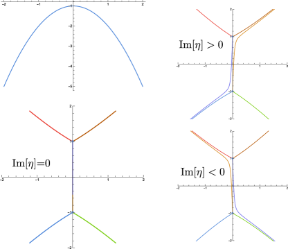
Figure 1: The potential $V(t)=-1-t^{2}$ ($E=0$) is shown on the upper left panel, in which the horizontal axis is real $t$. Other panels are the Stokes lines for Im$[\eta]=0$ (lower left), Im$[\eta]>0$(upper right) and Im$[\eta]<0$(lower right) shown on the complex $t$-plane. The Stokes lines have degenerated for Im$[\eta]=0$ and there is a gap between Im$[\eta]>0$ and Im$[\eta]<0$. The MTP structure has turning points at $t=\pm i$.

Assuming $E=k^{2}>0$, the connection matrix starting from $t=-\infty$ to $t=+\infty$ can be calculated using the EWKB, which gives (See Ref.Enomoto:2020xlf for calculational details)

$$\left(\begin{array}[]{cc}N^{2}\left(e^{-K_{ud}}+e^{K_{ud}}\right)&-ie^{-K_{ud}}\\ ie^{-K_{ud}}&\frac{e^{-K_{ud}}}{N^{2}}\\ \end{array}\right),$$ (28)

where we defined

$$K_{ud} \equiv \int^{t_{*}^{-}}_{t_{*}^{+}}S_{odd}dt$$ (29)

for $t_{*}^{\pm}\equiv\pm i\frac{k}{g_{2}v}$. To make the diagonal elements consistent, one may put a condition on the normalization factor $N$;

$$|N|^{-2}=\sqrt{1+e^{2K_{ud}}}.$$ (30)

Finally, the connection matrix becomes

$$\left(\begin{array}[]{cc}\sqrt{1+e^{-2K_{ud}}}&-ie^{-K_{ud}}\\ ie^{-K_{ud}}&\sqrt{1+e^{-2K_{ud}}}\\ \end{array}\right).$$ (33)

The result is consistent with the exact result obtained from the Weber function Enomoto:2020xlf .

The Schwinger effect can also be discussed in the same way Schwinger:1951nm ; Haro:2010mx ; Taya:2020dco ; Kitamoto:2020tjm ; Martin:2007bw ; Dumlu:2010ua . Consider a complex charged scalar field interacting with an electromagnetic field with the vector potential (constant electric field $E_{z}=E$)

$$A_{\mu}(t) = (0,0,0,-Et),$$ (34)

one will have

$$\hbar^{2}\frac{d^{2}\phi_{\mathbf{k}}}{c^{2}dt^{2}}+\left[m^{2}c^{2}+\left(\mathbf{p}-\frac{q}{c}\mathbf{A}(t)\right)^{2}\right]\phi_{\mathbf{k}} = 0,$$ (35)

which gives for the EWKB,

$$Q(t) = -m^{2}c^{4}-c^{2}\left(\mathbf{p}-\frac{q}{c}\mathbf{A}(t)\right)^{2}.$$ (36)

Using the EWKB, the Stokes lines can be easily drawn (changing the variable result in a simple form Haro:2010mx ) and the connection matrix of the solutions can be calculated. See also the exact solution given by the parabolic cylinder functions in Ref.Haro:2010mx . This situation is exactly the same as the cosmological particle production in the preheating model Kofman:1997yn . In the above equation, particle production appears to be a local event at a specific time, but given gauge symmetry, the time is arbitrary as long as the electric field is constant. See also Ref.Dumlu:2010ua for a discussion of the Stokes phenomena and Schwinger pair production in time-dependent laser pulses. Given the similarity between the Schwinger effect and Hawking radiation Frolov:1998wf , it seems quite natural that the Stokes phenomenon in Hawking radiation must be explained by a similar Stokes phenomenon in the temporal part. However, to the best of our knowledge, such a Stokes phenomenon has not been discussed yet in past studies. In this paper, we will show how the Stokes phenomenon appears in the Unruh effect and apply it to Hawking radiation.

2.1 The Stokes phenomena of the Unruh effect

Let us take a quick look at how the Stokes lines of the Unruh effect look in Rindler coordinates; in the WKB formalism, the spatial and temporal part can be separated. Here we consider a two-dimensional Rindler metric Birrell:1982ix

$$ds^{2} = -\left(1+\frac{ax_{R}}{c^{2}}\right)^{2}c^{2}dt_{R}^{2}+dx_{R}^{2}.$$ (37)

Assuming $c=1$, corresponding EWKB formulation has the space part given bySingleton:2013

$$Q(x_{R})=-\frac{E^{2}-m^{2}(1+ax_{R})^{2}}{(1+ax_{R})^{2}},$$ (38)

where two turning points and a pole appear at $x_{R}=(\pm E/m-1)/a$ and at the midpoint $x_{R}=-1/a$ (at the center of the loop structure of the Stokes lines in Fig.2). ($E$ in the scalar field equation must be discriminated form $E$ in the “Schwinger equation”.) In the $m\rightarrow 0$ limit, these turning points will flow to infinity. Since no Stokes line exists within the loop structure, the Stokes phenomenon is not expected in the space part. The “potential” and the Stokes lines are shown in Fig.2. Although there is no Stokes phenomenon in the space part of $x_{R}$, the “tunneling amplitude” at the pole (on the horizon) introduces $e^{-\pi\omega/2a}$. As discussed in Ref.Akhmedova:2008dz ; Singleton:2013 , the Unruh effect is accounted for using the WKB/tunneling method, but this calculation had a factor two problem. In Ref.Akhmedova:2008dz ; Singleton:2013 , a resolution of this discrepancy was advocated, in which authors pointed out that a time part contribution gives Im$[\omega\Delta t]=-\pi\omega/a$ upon crossing the horizon, where the time and the space coordinates reverse their time-like/space-like character. Using them as global analytic conditions Birrell:1982ix ; Frolov:1998wf ; Nakamura:2007vp and comparing the modes of inertial vacuum with the modes of an accelerating observer, one will find the Unruh effect.

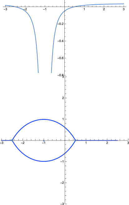
Figure 2: The upper panel is the “potential” of $Q(x_{R})=-\frac{E^{2}-m^{2}(1+ax_{R})^{2}}{(1+ax_{R})^{2}}$ for $a=1,E=0.3,m=0.2$ plotted for real $x_{R}$ (horizontal axis), and the lower panel shows the Stokes lines on the complex $x_{R}$ plane. A pole is shown at the center of the loop.

Since the Unruh effect is a local event, it is natural to expect that its information must be encoded in the local coordinate system. To understand what the observer sees in the inertial vacuum, we write a pair of $e^{\pm i\int\omega dt}$ solutions of the inertial observer’s vacuum using the accelerating observer’s time ($\tau$). The point of our observation is that $t$ is curved with respect to $\tau$, and such curvature can often introduce the Stokes phenomena.

Considering $ct=\frac{c^{2}}{a}\sinh\left(\frac{a}{c}\tau\right)$, we find $dt=\cosh\left(\frac{a}{c}\tau\right)d\tau$. Using $\alpha\equiv a/c$, we have

$$e^{\pm i\int\omega dt} = e^{\pm i\int\omega\cosh(\alpha\tau)d\tau},$$ (39)

which corresponds to the EWKB formalism with

$$\eta^{2}Q(\tau) = -\omega^{2}\cosh^{2}(\alpha\tau).$$ (40)

Here we have skipped the formal WKB expansion. Formally, one has to solve the differential equation using the WKB expansion. The equation is trivial for $t$ but it becomes non-trivial after changing the variable from $t$ to $\tau$. Considering a local series expansion of $Q(\tau)$ around $\tau=0$

$$\eta^{2}Q(\tau) = -\omega^{2}\cosh^{2}(\alpha\tau)$$ (41)

$$\simeq -\omega^{2}-\alpha^{2}\omega^{2}\tau^{2},$$

one can expect that the Stokes lines will form an MTP structure around $\tau=0$. The Stokes phenomenon of the MTP structure gives mixing of $\pm t$ (i.e, $\pm\tau$) solutions with $|e^{K_{ud}}|^{2}=e^{-\pi\omega/\alpha}$. Note that in the local coordinate system around $\tau=0$, we also have the expansion

$$\omega t = \omega\left(\frac{1}{\alpha}\sinh(\alpha\tau)\right)\simeq\omega\tau.$$ (42)

See also the remark on page 47 of Ref.Birrell:1982ix .

The structure of the Stokes lines is shown in Fig.3, which is the MTP structure surrounded by a pair of Stokes lines.

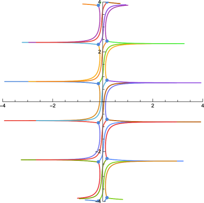
Figure 3: The Stokes lines for $Q(\tau)=-(\cosh^{2}2\tau+0.1+0.1i)(1+0.1i)$ are shown on the complex $\tau$ plane. The double turning points and the degenerated Stokes lines are both split by introducing small parameters. Note however that imaginary $\eta$ alone cannot solve all the degeneracy of this model.

Because of the Lorentz symmetry, $\tau=0$ is not special as far as $a$ is constant.

As we have mentioned previously, naive application of the Schwinger effect to the Unruh effect requires a factor of two. Our calculation of the local coordinate system gives $e^{-\pi\omega/\alpha}$ but the Unruh effect requires $e^{-2\pi\omega/\alpha}$. This indicates that the same problem occurs in our calculation. This result is not surprising since both calculations are local and the effect of the horizon is disregarded. In the next section, we will look at some details of the argument to see that this problem does not appear in Hawking radiation if the Hawking’s tunneling picture is properly incorporated.

2.2 The Stokes phenomena of Hawking radiation

We are going to see the Stokes phenomena of the modes that are defined with respect to the Killing time but viewed from an observer fixed at the horizon. Then, the local coordinate system would exhibit the Stokes phenomenon similar to the Schwinger effect. Despite their similarities, there is a very important difference between them. If a pair of particles is on the same side of the horizon, their total energy does not vanish, so this process is prohibited by the law of conservation of energy. Since the negative energy state must be located inside the horizon and its pair state must be outside, the production of observable (not virtual) particles must occur very close to the horizon (at least within Compton length of the particles), and only half of the created particles can be seen as “radiation from the horizon”. Since the Killing horizon in static spacetime is known to be the event horizon, (not virtual) particle production in a static gravitational system is only possible at the event horizon. In the case of black hole radiation, particle production must be pair production, and only half of the particles are observed. Then, the probability of particle production in the radiation must be squared, and an additional factor of two is introduced into the coefficient to obtain the correct Hawking temperature.

As mentioned earlier, the Stokes phenomena are not found in the space part of the WKB formalism, but they are found in the time part. Our idea is simple and straight. Since the Stokes phenomena of the Schwinger effect for a constant electric field are found in the time part Haro:2010mx , it is quite natural to expect that the Stokes phenomena of Hawking radiation must also be found in the time part, even though both models have “static” backgrounds. Our speculation was correct. The Stokes phenomena in the time part successfully explained Hawking radiation.

On the other hand, Giovanazzi Giovanazzi:2004zv found that a microscopic description of the space part of a sonic black hole explains the picture of “Hawking radiation as the tunneling”. Since Giovanazzi’s explanation of the tunneling conjecture implicitly uses the Stokes phenomena at the horizon, it must be important to compare these models in light of the Stokes phenomena. To explicitly show the difference between them, the next section describes the Stokes phenomena of the sonic black hole in some detail.

2.3 The Stokes phenomena of a sonic black hole

Considering a one-dimensional Fermi-degenerate liquid squeezed by a smooth barrier forming a transonic flow, Giovanazzi Giovanazzi:2004zv presented a microscopic description of Hawking radiation in sonic black holes.

The fundamental equations of fluid dynamics for an inviscid fluid in one dimension are the equation of continuity and Euler’s equation given by

$$\partial_{t}\rho\partial_{x}(\rho v) = 0$$

$$\rho(\partial_{t}v+v\partial_{x}v) = -\partial_{x}p-\frac{\rho}{m}\partial_{x}V(x),$$ (43)

where $\rho(t,x)$, $v(t,x)$, $p(t,x)$, $m$ and $V(x)$ are the density, velocity of flow, pressure, mass of a particle, and external potential of the particle, respectively. Then expand $\rho$ and $v$ as

$$\rho = \rho_{0}+\epsilon\rho_{1}+\epsilon^{2}\rho_{2}+...,$$

$$v = \rho_{0}+\epsilon v_{1}+\epsilon^{2}v_{2}+...,$$ (44)

where $\rho_{0}$ and $v_{0}$ denote the background flow, and $\rho_{i}$ and $v_{i}$ are giving the sound waves. Introducing the velocity potential $\phi$ such that $v_{1}=-\partial_{x}\phi$, one will find

$$\partial_{\mu}g^{\mu\nu}\partial_{\nu}\phi = 0,$$ (45)

where $\mu,\nu=t,x$. Here the “acoustic metric” is given by

$$g_{\mu\nu} = \frac{c_{s}^{2}}{\rho_{0}^{2}}\left(\begin{array}[]{cc}c_{s}^{2}-v_{0}^{2}&v_{0}\\ v_{0}&-1\end{array}\right),$$ (48)

where

$$c_{s} \equiv \sqrt{\frac{\partial p}{\partial\rho}}.$$ (49)

Choosing an appropriate potential $V(x)$, one will find that Hawking radiation is realized at the sound horizon which divides regions of $v_{0}<c_{s}$ and $v_{0}>c_{s}$. The temperature of the radiation at the horizon is

$$T=\frac{\hbar c_{s}}{4\pi k_{B}}\frac{\partial}{\partial x}\left(1-\frac{v_{0}^{2}}{c_{s}^{2}}\right)$$ (50)

Giovanazzi presented a microscopic description of Hawking radiation of sonic black holes in Ref.Giovanazzi:2004zv . A one-dimensional Fermi-degenerate liquid squeezed by a smooth barrier $V=-\frac{1}{2}\lambda x^{2}$ forms a transonic flow. Using $p=\hbar^{2}\pi^{2}\rho^{3}/3m^{4}$ for the Fermi-degenerate liquid and classical solutions

$$\rho_{0} = \frac{m}{2\pi\hbar}\left(\sqrt{2m(E_{F}+\lambda x^{2}/2)}-\sqrt{m\lambda}x\right)$$

$$v_{0} = \frac{1}{2m}\left(\sqrt{2m(E_{F}+\lambda x^{2}/2)}+\sqrt{m\lambda}x\right),$$ (51)

where $E_{F}$ is the energy of a particle on the Fermi surface, one will see that the sound horizon appears at $x=0$. Here the sound velocity is given by $c_{s}=\hbar\pi\rho_{0}/m^{2}$. After quantization, one will find that the temperature of Hawking radiation is given by

$$T=\frac{\hbar}{2\pi k_{B}}\sqrt{\frac{\lambda}{m}}.$$ (52)

By choosing $\lambda=m\omega_{x}^{2}$, we have

$$T=\frac{\hbar\omega_{x}}{2\pi k_{B}}.$$ (53)

Giovanazzi’s microscopic treatment of the quantum process shows a close relationship between sonic Hawking radiation and quantum tunneling (and quantum scattering) through the barrier.

To be more specific about the quantum processes, particles with $E>0$ radiate positive energy via quantum scattering (back outward the horizon), while particles with $E<0$ can tunnel the horizon barrier and enter the black hole. These quantum processes seem to explain Hawking’s original idea of “Hawking radiation as tunneling”. The temperature of the radiation given by Eq.(53) will be calculated either using special functions or from $e^{K_{ud}}$ of the EWKB, since this problem is nothing more than scattering by an inverted quadratic potential.

On the other hand, a comparison of this model with our calculation of the Stokes phenomena of the black hole shows a critical discrepancy between them.

3 How to include quantum backreactions in the EWKB

To illustrate the quantum correction to the Stokes phenomenon of Hawking radiation in the EWKB formalism, we first consider Hawking radiation from the sonic black hole. The result in this section can be easily applied to the Stokes phenomenon of black hole radiation. This is because in both cases the Stokes phenomena are explained by the MTP structure of the inverted quadratic potential. Given that Hawking radiation is described by the Stokes phenomenon of the local time coordinate system, the only parameter required for the Stokes phenomenon is the local surface gravity. Following Ref.Giovanazzi:2004zv , we consider the EWKB with a potential $V(x)=-\frac{1}{2}ma^{2}x^{2}$, which gives the temperature of the sonic black hole

$$T = \frac{\hbar}{2\pi k_{B}}a.$$ (54)

To compare the sonic black hole and the conventional Hawking radiation, we have relations

$$a \rightarrow \frac{c^{3}}{4GM}$$

$$\dot{M} = \frac{\hbar c^{4}}{15360\pi G^{2}}\frac{1}{M^{2}},$$ (55)

where we set $G$ and $M$ are the gravitational constant and the black hole mass, respectively. We also have $\dot{a}\propto\dot{M}/{M^{2}}\propto M^{-4}\hbar\propto a^{4}\hbar$.

For a real black hole, the radiation continuously takes away the mass of the black hole. Then, what an observer sees as the black hole mass depends on the distance from the horizon. To realize the same phenomenon in the sonic black hole, we consider a snapshot of the black hole and introduce $a(x)\simeq a_{0}+f(\hbar,x)$, where $a_{0}$ is defined at the horizon ($x=0$). Then the quantum correction can be expanded as

$$f(x,\hbar) = \sum^{\infty}_{j=1}\hbar^{j}f_{j}(x).$$ (56)

Now the problem becomes scattering by a potential

$$V(x,\hbar) = -\frac{m}{2}a_{0}^{2}x^{2}-\frac{m}{2}\sum^{\infty}_{j=1}\hbar^{j}f_{j}(x).$$ (57)

For the EWKB, we have

$$Q(x)_{0} = -E-\frac{m}{2}a_{0}^{2}x^{2},$$

$$Q(x)_{j} = -\frac{m}{2}f_{j}(x),$$ (58)

where $j\geq 1$. Then, what we have to do is (1) Draw the Stokes lines using $Q_{0}$ and (2) Calculate the $\hbar$-correction of the observables. Since the Stokes lines are defined by $Q(x)_{0}$, the Stokes lines are identical to the original model and quantum corrections must appear only in $K_{ud}$.

4 Conclusions and discussions

In this paper, the EWKB analysis and the Stokes phenomena are used to analyze the Unruh effect and Hawking radiation. The similarity between the Schwinger effect and the Unruh effect (Hawking radiation) has often been mentioned in textbooks, but there has been no clear explanation of the common Stokes phenomenon. Also, the Unruh effect and Hawking radiation seem to be local phenomena. To address these issues, we focused on the Schwinger effect in a constant electric field and examined its similarity to the Unruh effect and Hawking radiation. Writing down the modes of the inertial vacuum using the observer’s time, we found the Stokes phenomenon in the local time coordinate system. The calculation gives the correct Hawking temperature.

We then compared our analysis of the black hole with an analog black hole and found a crucial discrepancy between them.

To show why the exact $\hbar$ expansion is important for semiclassical calculations, we have briefly described how Hawking radiation is altered by the quantum radiation.

An application of these results is a bound on chaos Maldacena:2015waa . In order to investigate the chaos bound of a quantum system in detail, it is useful to investigate the Stokes phenomenon causing the quantum radiation. At the same time, an accurate way to describe the relationship between classical and quantum effects is needed Morita:2019bfr ; Shudo:2016 . In this paper, the Stokes phenomenon of Hawking radiation is analyzed with the EWKB, where the EWKB provides a way to describes the relationship between the classical and quantum theoretical effects in an accurate way, in the sense that its $\hbar$ expansion is rigorous.