The Exact WKB analysis for asymmetric scalar preheating

Abstract

Using the exact WKB analysis of the higher-order differential equations, we analyze the asymmetry in dynamical particle production of a complex scalar field. The solution requires the Stokes phenomena of the fourth-order differential equation. We found that the interference of different types of the Stokes phenomena causes matter-antimatter asymmetry. We also showed a specific example where asymmetry is forbidden in the exact calculation, but a false asymmetry appears in the perturbative expansion.

1 Introduction

One of the most important physical parameters of the Universe is the observed ratio of the baryon number density to photon density. The Planck resultPlanck:2018vyg suggests that the ratio is given byParticleDataGroup:2020ssz

$$n_{B}/n_{\gamma} = (6.12\pm 0.04)\times 10^{-10}.$$ (1)

The theoretical and phenomenological approach to explaining the ratio is called baryogenesis, which is usually based on Sakharov’s three conditionsSakharov:1967dj : (1) non-conservation of baryon number, (2) breaking of C and CP invariance, (3) deviation from thermal equilibrium. However, some interesting models of baryogenesis do not fit into Sakharov’s scenario. The model, which is called “spontaneous baryogenesis”, proposed the essential idea of such scenariosCohen:1987vi ; Cohen:1988kt ; Cohen:1991iu . The term “spontaneous” means spontaneous breaking of underlying symmetry (e.g, the global $U(1)$ symmetry of the conservation of the baryon number), which leads to

$${\cal L}_{sb} \sim (\partial_{\mu}\theta)J^{\mu}_{B},$$ (2)

where $\theta$ is the phase of a field, and the phase is related to the (pseudo) Nambu-Goldstone field of the symmetry. $J^{\mu}_{B}$ is the corresponding current. The point of their observation is that the above interaction can lead to nonconservation of the baryonic current of matter, but the nonconservation disappears when $\theta$ is neither inhomogeneous nor time-dependent. Normally, the term in Eq.(2) is identified with the chemical potential in the Hamiltonian density by using the relation

$${\cal H}_{chem}=-{\cal L}_{sb},$$ (3)

but this is not an obvious relation, as is discussed in Ref.Arbuzova:2016qfh . We will see shortly the point of Ref.Arbuzova:2016qfh in Sec.1.1.

The idea of spontaneous baryogenesis can be found in the Affleck-Dine baryogenesisAffleck:1984fy , which is one of the most popular scenarios of baryogenesis. The Affleck-Dine baryogenesis considers rotational motion of a field, which implies generation of the baryon number. Because of spatial instabilities of the Affleck-Dine field, the produced baryon number ($Q$) is believed to form Q-ballsKasuya:1999wu ; Enqvist:1998en .

An important aspect of our analysis is that these models consider a dynamical (time-dependent) scalar field with rotational motion, whereas the dynamical production of particles due to such motion has not been discussed using the Stokes phenomena. The term "dynamical particle production" here refers to particle generation from a vacuum, which is described using the Bogoliubov coefficients and the Stokes phenomena (mixing of solutions of a differential equation). Let us now look at the details of this problem by reviewing previous works. Since the emphasis in this paper is on identifying the origin of the asymmetry, the discussion is entirely qualitative.

1.1 The role of the chemical potential in dynamical particle production

The spontaneous baryogenesis scenario considers Eq.(2) to introduce the matter-antimatter asymmetry, but the validity of the identification (3) is questionableArbuzova:2016qfh . The point of the argument is that the transformation with respect to the “dynamical” fields $\phi_{a}$ and their canonical momentum conjugate $\pi_{a}={\partial\cal L}/{\partial\dot{\phi}_{a}}$ gives

$${\cal H}=\sum_{a}\pi_{a}\dot{\phi}_{a}-{\cal L}.$$ (4)

Applying the rule to the “field” $\theta$ with ${\cal L}_{sb}$, one cannot find the “chemical potential” because of $\pi_{\theta}$. As is described in Ref.Arbuzova:2016qfh , it could be possible to find a contribution similar to the chemical potential, but the process is far from trivial.

On the other hand, assuming that the field in motion is an external field, for which the momentum conjugate $\pi_{\theta}$ can be neglected, one will immediately find the desired “chemical potential” in the Hamiltonian.

Since the above situation is almost the same for fermionsArbuzova:2016qfh , it is natural to think that the “chemical potential” used in the spontaneous baryogenesis scenario requires further study. For us, this point is one of the primary reasons for considering original equations of motion for particle production instead of using an effective theory.

Let us see the meaning of the “chemical potential” of the spontaneous baryogenesis scenario in more detail. Suppose that the field in motion can be regarded as an external field. In that case, we knowArbuzova:2016qfh that ${\cal L}_{SB}$ can introduce the conventional chemical potential in the Hamiltonian formalism. Then, a naive question arises. “Does this chemical potential bias dynamical particle production ?” The answer to this naive question is far from trivial. To find an answer (not a no-go theorem) to this question, consider a simple solution of a bosonic field when ${\cal L}_{SB}$ has a constant and homogeneous $\mu\equiv\dot{\theta}$. In contrast to naive speculation, this model does not allow chemical potentials to bias particle production.

Consider the simplest scenario of bosonic preheating given by the actionEnomoto:2017rvc

$$S_{0} = \int d^{4}x\sqrt{-g}\left[\partial_{\mu}\phi^{*}\partial^{\mu}\phi-m^{2}|\phi|^{2}+\xi R|\phi|^{2}\right].$$ (5)

Using conformal time $\eta$, one can write the metric $g_{\mu\nu}=a^{2}(\eta){\rm diag}(1,-1,-1,-1)$ and $R=-6\ddot{a}/a^{3}$, where $a$ is the cosmological scale factor and the dot denotes time-derivative with respect to the conformal time. Defining a new field $\chi\equiv a\phi$, one will find a simple form

$$S_{0} = \int d^{4}x\left[|\dot{\chi}|^{2}-\omega^{2}|\chi|^{2}\right],$$ (6)

where

$$\omega^{2} \equiv a^{2}m^{2}+\left(-\Delta+\frac{\ddot{a}}{a}(6\xi-1)\right).$$ (7)

Here $\Delta$ is the Laplacian. Annihilation ($a,b$) and creation ($a^{\dagger},b^{\dagger}$) operators of “particle” and “antiparticle” appear in the standard decomposition

$$\chi = \int\frac{d^{3}k}{(2\pi)^{3/2}}\left[h(\eta)a(\bm{k})e^{i\bm{k}\cdot\bm{x}}+g^{*}(\eta)b^{\dagger}(\bm{k})e^{-i\bm{k}\cdot\bm{x}}\right].$$

For our calculation, we introduce conjugate momenta $\Pi^{\dagger}\equiv\dot{\chi}$, which can be decomposed as

$$\Pi^{\dagger} = \int\frac{d^{3}k}{(2\pi)^{3/2}}\left[\tilde{h}(\eta)a(\bm{k})e^{i\bm{k}\cdot\bm{x}}+\tilde{g}^{*}(\eta)b^{\dagger}(\bm{k})e^{-i\bm{k}\cdot\bm{x}}\right].$$

Following Ref.ZS-original , we expand $h,\tilde{h}$ (particles) and $g,\tilde{g}$ (antiparticles) as

$$h = \frac{e^{-i\int^{\eta}\omega d\eta^{\prime}}}{\sqrt{2\omega}}A_{h}+\frac{e^{i\int^{\eta}\omega d\eta^{\prime}}}{\sqrt{2\omega}}B_{h},$$

$$\tilde{h} = \frac{-i\omega e^{-i\int^{\eta}\omega d\eta^{\prime}}}{\sqrt{2\omega}}A_{h}+\frac{i\omega e^{i\int^{\eta}\omega d\eta^{\prime}}}{\sqrt{2\omega}}B_{h},$$ (10)

and

$$g = \frac{e^{-i\int^{\eta}\omega d\eta^{\prime}}}{\sqrt{2\omega}}A_{g}+\frac{e^{i\int^{\eta}\omega d\eta^{\prime}}}{\sqrt{2\omega}}B_{g},$$

$$\tilde{g} = \frac{-i\omega e^{-i\int^{\eta}\omega d\eta^{\prime}}}{\sqrt{2\omega}}A_{g}+\frac{i\omega e^{i\int^{\eta}\omega d\eta^{\prime}}}{\sqrt{2\omega}}B_{g},$$ (11)

where $A_{h,g}$ and $B_{h,g}$ are known as the Bogoliubov coefficients. (To avoid confusion, we are following the notations used in Ref.Enomoto:2017rvc , which are slightly different from the ones used in this paper.) For further simplification, we introduce $\alpha_{h,g}$ and $\beta_{h},g$, which are defined as

$$\alpha_{h,g} \equiv e^{-i\int^{\eta}\omega d\eta^{\prime}}A_{h,g}$$ (12)

$$\beta_{h,g} \equiv e^{i\int^{\eta}\omega d\eta^{\prime}}B_{h,g}.$$ (13)

Now the equation of motion can be written as

$$\dot{h}-\tilde{h} = 0$$ (14)

$$\dot{\tilde{h}}+\omega^{2}h = 0,$$ (15)

which are solved for $\dot{\alpha}$ and $\dot{\beta}$ as

$$\dot{\alpha}_{h} = -i\omega\alpha_{h}+\frac{\dot{\omega}}{2\omega}\beta_{h}$$

$$\dot{\beta}_{h} = i\omega\beta_{h}+\frac{\dot{\omega}}{2\omega}\alpha_{h}.$$ (16)

The same calculation gives $\dot{\alpha}_{g}$ and $\dot{\beta}_{g}$.

Let us see what happens when a constant chemical potential is introduced. After adding a chemical potential

$${\cal L} = \dot{\chi}\dot{\chi}^{*}-\omega^{2}|\chi|^{2}-i\mu_{\chi}\left(\chi\dot{\chi}^{*}-\chi^{*}\dot{\chi}\right),$$ (17)

we find

$$\ddot{\chi}-2i\mu_{\chi}\dot{\chi}+(\omega^{2}-i\dot{\mu}_{\chi})\chi = 0.$$ (18)

Two terms that might cause differences between $h$ and $g$ are $-2i\mu_{\chi}\dot{\chi}$ and $-i\dot{\mu}_{\chi}\chi$. If one assumes constant chemical potential, only the first term will remain.

As we have noted above, one can verify that the constant chemical potential does not generate asymmetry in this model. Here, the equation of motion becomes

$$\dot{h}-\tilde{h}-i\mu_{\chi}h = 0$$

$$\dot{\tilde{h}}+\omega^{2}h-i\mu_{\chi}\tilde{h} = 0.$$ (19)

One can solve these equations for $\dot{\alpha}$ and $\dot{\beta}$ to find

$$\dot{\alpha}_{h} = -i(\omega-\mu_{\chi})\alpha_{h}+\frac{\dot{\omega}}{2\omega}\beta_{h}$$

$$\dot{\beta}_{h} = \frac{\dot{\omega}}{2\omega}\alpha_{h}+i(\omega+\mu_{\chi})\beta_{h}.$$ (20)

The same calculation for $g$ gives

$$\dot{\alpha}_{g} = -i(\omega+\mu_{\chi})\alpha_{g}+\frac{\dot{\omega}}{2\omega}\beta_{g}$$

$$\dot{\beta}_{g} = \frac{\dot{\omega}}{2\omega}\alpha_{g}+i(\omega-\mu_{\chi})\beta_{g}.$$ (21)

One might be tempted to speculate that the shift of $\omega\pm\mu_{\chi}$ will bias the particle production, but this speculation fails in the present model. Using a simple calculation of $\frac{d|\beta_{h}|^{2}}{dt}$ and $\frac{d|\beta_{h}|^{2}}{dt}$, one can verify that the evolution of $|\beta_{h}|^{2}$ and $|\beta_{g}|^{2}$ are identical in this case, resulting in no asymmetry production. See ref.Enomoto:2017rvc for more details.

We have seen that the chemical potential may not bias particle production even if the field in motion is regarded as an external field. The above calculation also indicates that $\dot{\mu}\neq 0$ may resolve the degeneracy. See also RefsKusenko:2014uta ; Pearce:2015nga ; Adshead:2015jza ; Adshead:2015kza ; Enomoto:2021hfv for recent discussions on this topic. In fact, when considering chemical potentials in cosmology, they should be time-dependent, since $\mu$ is usually defined using a time-dependent parameter. Of course, if we consider the chemical potential of the external field in a system of Boltzmann equations, the complications described above for dynamical particle production do not appear; see also Refs.Kusenko:2014lra ; Yang:2015ida ; Wu:2019ohx for a recent discussion on the Higgs relaxation.

The rotational motion of a scalar field can be seen not only at the preheating stage of natural inflationFreese:1990rb ; Adams:1992bn , but also inside Q-ballsColeman:1985ki ; Kusenko:1997si or other cosmological defects in motionLiu:1992tn ; Matsuda:2002br ; Matsuda:2001yi . Particles generated by the oscillation will decay when it obtains a large mass from the oscillating field, breaking the coherent growth. If the particles do not decay, there could be “trapping”Kofman:2004yc ; Enomoto:2013mla of the oscillating field, which makes the global calculation chaotic. In this paper, we do not discuss the quantitative calculation but focus on the local event and seek the origin of the asymmetry.

1.2 Asymmetry in preheating scenarios

When fundamental parameters such as mass and interaction coefficients become time-dependent, particles can be produced from the vacuum, and there are various reasons why fundamental parameters can change during cosmological evolution. Among them, particle production by inflaton oscillations is known to be very important for solving the problem of reheating the universe after inflation.Traschen:1990sw ; Kofman:1997yn ; Felder:1998vq ; Kofman:2004yc .

A semiclassical calculation of fermionic particle production by a Nambu-Goldstone boson is performed in Ref.Dolgov:1994zq . They started with a simple model for a complex scalar field $\Phi$ and two fermions $Q$ and $L$:

$$S = \int d^{4}x\left[g^{\mu\nu}\partial_{\mu}\Phi^{*}\partial_{\nu}\Phi-V(\Phi^{*}\Phi)\right.$$ (22)

$$\left.+i\overline{Q}\gamma^{\mu}\partial_{\mu}Q+i\overline{L}\gamma^{\mu}\partial_{\mu}L+(g\Phi\overline{Q}L+h.c.)\right].$$

This action is invariant under a $U(1)$ symmetry. In Ref.Dolgov:1994zq , they have chosen

$$\Phi\rightarrow e^{i\alpha}\Phi, Q\rightarrow e^{i\alpha}Q, L\rightarrow L.$$ (23)

To introduce spontaneous breaking of the global symmetry, the potential is as

$$V(|\Phi|) = \lambda\left[\Phi^{*}\Phi-f^{2}/2\right]^{2},$$ (24)

which gives

$$\langle\Phi\rangle = fe^{i\phi/f}/\sqrt{2}$$ (25)

Just for simplicity of notation, the dimensionless angular field $\theta\equiv\phi/f$ has been introduced to obtain the effective Lagrangian for $\theta$:

$${\cal L} = \frac{f^{2}}{2}\partial_{\mu}\theta\partial^{\mu}\theta+i\overline{Q}\gamma^{\mu}\partial_{\mu}Q$$ (26)

$$+i\overline{L}\gamma^{\mu}\partial_{\mu}L+(gf\overline{Q}Le^{i\theta}+h.c.),$$

where the global symmetry is realized as

$$\theta\rightarrow\theta+\alpha, Q\rightarrow e^{i\alpha}Q, L\rightarrow L.$$ (27)

For $\alpha=-\theta$, one can rewrite the Lagrangian as

$${\cal L} = \frac{f^{2}}{2}\partial_{\mu}\theta\partial^{\mu}\theta+i\overline{Q}\gamma^{\mu}\partial_{\mu}Q+i\overline{L}\gamma^{\mu}\partial_{\mu}L$$ (28)

$$+(gf\overline{Q}L+h.c.)+\partial_{\mu}\theta J^{\mu}-U(\theta),$$

where $J^{\mu}=\overline{Q}\gamma^{\mu}Q$ denotes the fermion current of the $U(1)$ symmetry, and $U(\theta)$ is assumed to be given by

$$U(\theta) = \Lambda^{4}\left[1\pm\cos\theta\right].$$ (29)

Note that the model is inspired by the model of natural inflationFreese:1990rb ; Adams:1992bn and aims to propose baryogenesis caused by the preheating stage after natural inflation.

The baryon number asymmetry generated by the Pseudo-Nambu Goldstone Boson(PNGB) was calculated in Ref.Cohen:1987vi . Their result is $|\dot{n}_{B}|=\Gamma f^{2}|\dot{\theta}|$, where $\Gamma$ is the decay rate of the PNGB. However, the authors of Ref.Dolgov:1994zq alerted that the original calculation might be naive. Note that a similar question may arise for the decay of the Affleck-Dine field and a Q-ball. In Ref.Dolgov:1996qq , they have expanded the calculation to find that the baryon number should be given by

$$n_{B} \propto \Gamma f^{2}\theta_{i}^{3},$$ (30)

where the $\theta$-dependence is modified. Their calculation in Ref.Dolgov:1996qq uses the Bogoliubov transformation and two different kinds of expansion: small $g$ and small $\theta(t)$. We will see later that the expansion of Ref.Dolgov:1996qq may destroy the structure of the Stokes lines, to change the qualitative analysis of the model. What is important in the approachDolgov:1996qq is that they have explicitly included interaction between different species $Q$ and $L$.

Before going forward, we explain why the exact WKB (EWKB) is crucial for dynamical particle production. The equations of motion become higher-order differential equations when an interaction is introduced. (See the model described above.) Global asymptotic analysis of the higher-order differential equations was thought to be impossible to construct before the discovery of the “new Stokes lines” by H.L. Berk, W.M. Nevins, and K.V. RobertsNBR . Later by T. Aoki, T. Kawai, and Y. TakeiVirtual:2015HKT , the notion of a virtual turning point was discovered by applying microlocal analysis to Borel transformed WKB solutions. Since the virtual turning point cannot be detected by ordinary WKB solutions, the conversion of the study to the one in a different space, the Borel plane on which the Borel transformed WKB solutions are analyzed, was indispensable. We are using these ideas to discuss matter-antimatter asymmetry in a scalar preheating scenario with complex time-dependent parameters.

We are aware that the EWKB analysis is not yet common; one may be puzzled by the claim that the Borel resummation of the WKB expansion is not an approximation but gives an exact result. One might also wonder why the Stokes lines in the EWKB analysis are giving an exact result when they are computed from the first term of the expansion. Also, Stokes phenomena in ordinary differential equations may not be a popular topic in cosmology. Therefore, to avoid confusion, we will review these topics in this paper. Our discussions in the review sections are based on our previous papersEnomoto:2020xlf ; Enomoto:2021hfv and the textbookVirtual:2015HKT . We also refer the reader to Ref.Taya:2020dco ; Kitamoto:2020tjm ; Hashiba:2021npn . On the other hand, we do not review the mathematical details of the formulation. For details and proofs, see Refs.Virtual:2015HKT ; Voros:1983 ; Delabaere:1993 . We only describe how to use this useful tool in a cosmological particle generation scenario.

1.3 The Stokes phenomena and the Bogoliubov transformation in cosmological particle creation

First, we explain why the Bogoliubov transformation is explained by the Stokes phenomena, applying them to the standard preheating scenario.

The motion of the inflaton field is a damped oscillation. However, at least near the center of the oscillation, where particle production is likely to take place, a linear approximation with respect to $t$ can be made. Typically, the mass of a scalar field (e.g, $\chi$) is supposed to be given by

$$m^{2}_{\chi}(t) = m_{0}^{2}+g^{2}_{2}\phi(t)^{2},$$ (31)

where $\phi(t)$ is the oscillating inflaton field. If we consider the Lagrangian given by

$${\cal L}_{\chi} = \frac{1}{2}\partial_{\mu}\chi\partial^{\mu}\chi-\frac{1}{2}m_{0}^{2}\chi^{2}-\frac{1}{2}g_{2}^{2}\phi(t)^{2}\chi^{2},$$ (32)

the equation of motion becomes

$$\frac{d^{2}\chi}{dt^{2}}+\left[k^{2}+m^{2}_{\chi}(t)\right]\chi=0.$$ (33)

If one replaces $\phi(t)$ with $\phi(t)\simeq vt$, the above equation is equivalent to the Schrödinger equation of the scattering problem. Following the mathematician’s formulation, in which “$m$” in the original Schrödinger equation is removed by setting “$2m=1$”, we define inverted quadratic “potential” given by

$$V(t) = -\left(g_{2}^{2}v^{2}\right)t^{2},$$ (34)

where the corresponding “energy” is

$$E = k^{2}+m_{0}^{2}.$$ (35)

Note that $E>V$ is always true in this case. Therefore, there is no classical turning point in the scattering problem.

There are a variety of methods for finding the wave functions of the general one-dimensional scattering problem of quantum mechanics. For the inverted quadratic potential, one can find the exact solution (i.e, the Weber function, or the parabolic cylinder functions). Analytic continuation of the WKB expansion (complex WKB) and related topics have a long historyPokrovskii:1961 . For instance, it has been applied to pair production in a vacuum by an alternating fieldBrezin:1970xf . Note however that without the Borel resummation the definitions of the WKB expansion and the analytic continuation are vague. The most obvious confusion will be that without the Bore resummation the Stokes lines seem to be changed by introducing higher terms. Therefore, the EWKB is crucial for our argument.

Since the model gives the typical structure of the Stokes lines (the so-called “Merged pair of simple Turning Points(MTP)”), we are going to show explicitly the calculation in detail.

Typically, the (conventional) WKB expansion is used to find

$$\chi_{k}(t) = \frac{\alpha_{k}(t)}{\sqrt{2\omega_{k}}}e^{-i\int^{t}\omega dt}+\frac{\beta_{k}(t)}{\sqrt{2\omega}}e^{+i\int^{t}\omega dt},$$ (36)

where

$$\omega^{2}_{k}(t) \equiv k^{2}+m_{\chi}^{2}(t).$$ (37)

Here $\alpha_{k}=1$ and $\beta_{k}=0$ are considered for the initial vacuum state. These solutions are the asymptotic states of the exact solutions for which the number densities are defined. (Of course, in cosmology one is not considering exact $t\rightarrow\pm\infty$ limits for the states. The Stokes phenomenon is a local event.) The distribution of the particle in the final state is

$$n_{\chi}(k)=|\beta_{k}|^{2},$$ (38)

which can be found by solving the scattering problem of the corresponding Schrödinger equation. The connection formulae of the solutions, which give $\beta_{k}\neq 0$ for the final state, are nothing but the consequence of the Stokes phenomena.

To see what happens, we are going to solve the equation of motion explicitly using the Weber function. For the above model (i.e, scattering by the inverted quadratic potential), the following Weber equation

$$y^{\prime\prime}(z)+\left(\nu+\frac{1}{2}-\frac{1}{4}z^{2}\right)y(z)=0$$ (39)

has the solution $D_{\nu}(z),D_{-\nu-1}(iz)$. More specifically, one can define

$$z \equiv ie^{i\pi/4}\sqrt{2g_{2}v}t$$ (40)

in the original field equation to find

$$\frac{d^{2}\chi}{dz^{2}}+\left[\nu+\frac{1}{2}-\frac{1}{4}z^{2}\right]\chi=0.$$ (41)

Here we defined

$$\nu=\frac{k^{2}+m_{0}^{2}}{2g_{2}v}i-\frac{1}{2},$$ (42)

and for later use we define

$$\kappa \equiv \frac{k^{2}+m_{0}^{2}}{2g_{2}v}$$ (43)

and

$$\nu=i\kappa-\frac{1}{2}.$$ (44)

Here, $\kappa$ is an important parameter, which is later used to estimate particle production. In the next section, we will show how to calculate $\kappa$ in the EWKB. The asymptotic forms of the Weber function at $|z|\rightarrow\infty$ are given by

$$1. |\mathrm{arg}z|<\frac{3\pi}{4}, \,\,D_{\nu}(z)\rightarrow e^{-z^{2}/4}z^{\nu},$$ (45)

$$2. -\frac{5}{4}\pi<\mathrm{arg}z<-\frac{\pi}{4}, \,\,D_{\nu}(z)\rightarrow e^{-\frac{z^{2}}{4}}z^{\nu}-\frac{\sqrt{2\pi}}{\Gamma(-\nu)}e^{-i\nu\pi+\frac{z^{2}}{4}}z^{-\nu-1},$$ (46)

$$3. \frac{\pi}{4}<\mathrm{arg}z<\frac{5\pi}{4}, \,\,D_{\nu}(z)\rightarrow e^{-\frac{z^{2}}{4}}z^{\nu}-\frac{\sqrt{2\pi}}{\Gamma(-\nu)}e^{i\nu\pi+\frac{z^{2}}{4}}z^{-\nu-1}.$$ (47)

Since $z\equiv ie^{i\pi/4}\sqrt{2g_{2}v}t$ is used here, $t<0$ gives $\frac{5\pi}{4}<\mathrm{arg}z<\frac{9\pi}{4}$, which corresponds to region 1. Also, $t\rightarrow+\infty$ corresponds to region 3. Therefore, we find for $t\rightarrow-\infty$,

$$e^{-\frac{z^{2}}{4}} = e^{-i\frac{g_{2}v}{2}t^{2}}$$ (48)

$$z^{\nu} = e^{(i\kappa-\frac{1}{2})\log z}$$ (49)

$$= e^{(i\kappa-\frac{1}{2})\left(\log(\sqrt{2g_{2}v}|t|)+i\frac{3\pi}{4}\right)},$$

which gives ($t=-|t|=e^{\pi i}|t|$ is used here)

$$D_{\nu}(z) \simeq e^{-i\frac{g_{2}v}{2}t^{2}}e^{(i\kappa-\frac{1}{2})\left(\log(\sqrt{2g_{2}v}|t|)-i\frac{\pi}{4}\right)},$$ (50)

$$D_{-\nu-1}(iz) \simeq e^{+i\frac{g_{2}v}{2}t^{2}}e^{(-i\kappa-\frac{1}{2})\left(\log(\sqrt{2g_{2}v}|t|)+i\frac{\pi}{4}\right)}.$$ (51)

Note that the above solutions in the limit $t\rightarrow-\infty$ are giving the $\pm$ WKB solutions of Eq.(36). Therefore, we define

$$\chi_{-} \rightarrow D_{\nu}(z)$$ (52)

$$\chi_{+} \rightarrow D_{-\nu-1}(iz).$$ (53)

On the other hand, in the $t\rightarrow+\infty$ limit, we find

$$e^{-\frac{z^{2}}{4}} = e^{-i\frac{g_{2}v}{2}t^{2}}$$ (54)

$$z^{\nu} = e^{(i\kappa-\frac{1}{2})\log z}$$ (55)

$$= e^{(i\kappa-\frac{1}{2})\left(\log(\sqrt{2g_{2}v}t)+i\frac{3\pi}{4}\right)},$$

which gives in this limit,

$$D_{\nu}(z) \simeq e^{-i\frac{g_{2}v}{2}t^{2}}e^{(i\kappa+\frac{1}{2})\left(\log(\sqrt{2g_{2}v}t)+i\frac{3\pi}{4}\right)}$$

$$+i\frac{\sqrt{2\pi}}{\Gamma(-\nu)}e^{i\frac{g_{2}v}{2}t^{2}}e^{-\kappa\pi}e^{(-i\kappa-\frac{1}{2})\left(\log(\sqrt{2g_{2}v}t)+i\frac{3\pi}{4}\right)}.$$

Immediately, one will find that in the $t=+\infty$ limit the asymptotic form of the exact solution $D_{\nu}(z)$ is the mixture of the $\pm$ WKB solutions, which gives the connection formula of the Stokes phenomena. In this case, the connection formula gives the Bogoliubov transformation of the WKB solutions. In the calculation of the connection formula, we use

$$\Gamma(z)\Gamma(1-z) = \frac{\pi}{\sin\pi z}$$ (57)

$$\Gamma(\bar{z}) = \overline{\Gamma(z)}$$ (58)

$$1+\nu = 1+\left(i\kappa-\frac{1}{2}\right)=-\overline{\nu}$$ (59)

for the calculation of $\Gamma(-\nu)=\Gamma(-i\kappa+\frac{1}{2})$. This gives

$$|\Gamma(-\nu)|^{2} = \frac{\pi}{\sin\pi(-\nu)}$$ (60)

$$= \frac{2\pi i}{e^{-i\pi\nu}-e^{i\pi\nu}}$$

$$= \frac{2\pi}{e^{\pi\kappa}+e^{-\pi\kappa}}$$

$$\Gamma(-\nu) = \frac{\sqrt{2\pi}e^{-\pi\kappa/2}}{\sqrt{1+e^{-2\pi\kappa}}}e^{\mathrm{arg}\Gamma(-\nu)}.$$ (61)

Finally, one obtains the connection formula given by

$$\left(\begin{array}[]{c}\alpha_{k}^{R}\\ \beta_{k}^{R}\end{array}\right) = \left(\begin{array}[]{cc}\sqrt{1+e^{-2\pi\kappa}}e^{i\theta_{1}}&ie^{-\pi\kappa+i\theta_{2}}\\ -ie^{-\pi\kappa-i\theta_{2}}&\sqrt{1+e^{-2\pi\kappa}}e^{-i\theta_{1}}\end{array}\right)\left(\begin{array}[]{c}\alpha_{k}^{L}\\ \beta_{k}^{L}\end{array}\right),$$ (68)

where L and R denote $t\rightarrow-\infty$ and $t\rightarrow+\infty$, respectively. Here, all phase parameters are put into $\theta_{1,2}(k)$. Viewing the result as the solution of the scattering problem, the reflection and the penetration amplitudes are given by

$$|R_{k}| = \frac{e^{-\pi\kappa}}{\sqrt{1+e^{-2\pi\kappa}}}$$

$$|T_{k}| = \frac{1}{\sqrt{1+e^{-2\pi\kappa}}}.$$ (70)

In the above scenario, there is no classical reflection point. This means that classically reflection is not allowed in the scattering problem. Therefore, particle production becomes significant when $\kappa\ll 1$, where the quantum scattering process becomes significant.

1.4 Introduction to the Exact WKB analysis

The Wentzel - Kramers - Brillouin - Jeffreys(WKB or WKBJ) approximation is a well-known method for solving linear differential equations. Although the first term of the expansion normally gives an excellent approximate solution, the method is formally giving a divergent power series. The Exact WKB analysis considers the Borel resummation to solve this problem. Thanks to the Borel resummation, the Borel sum is extended to the complex $\eta$-plane, where $\eta$ is the expansion parameter corresponding to $\hbar^{-1}$. Using these ideas of the EWKB, one can guarantee calculations of the WKB expansion avoiding the infamous problems of the original formulation.

The typical mathematician’s formulation of the EWKB uses $\eta\equiv\hbar^{-1}\gg 1$ instead of $\hbar$. Following Ref.Virtual:2015HKT , our starting point is the mathematician’s “Schrödinger equation” given by

$$\left[-\frac{d^{2}}{dx^{2}}+\eta^{2}Q(x)\right]\psi(x,\eta) = 0.$$ (71)

Introducing the “potential” $V$ and the “energy” $E$, we define

$$Q(x) = V(x)-E.$$ (72)

Writing the solution as $\psi(x,\eta)=e^{R(x,\eta)}$, we have

$$\psi = e^{\int^{x}_{x_{0}}S(x,\eta)dx}$$ (73)

for $S(x,\eta)\equiv\partial R/\partial x$. Here $x_{0}$ is an arbitrary parameter but normally taken on a turning point. For $S$, we have

$$-\left(S^{2}+\frac{\partial S}{\partial x}\right)+\eta^{2}Q = 0.$$ (74)

If one expands $S$ as $S(x,\eta)=\sum_{n=-1}^{n=\infty}\eta^{-n}S_{n}$, one will find

$$S=\eta S_{-1}(x)+S_{0}(x)+\eta^{-1}S_{1}(x)+...,$$ (75)

which leads

$$S_{-1}^{2} = Q$$ (76)

$$2S_{-1}S_{j} = -\left[\sum_{k+l=j-1,k\geq 0,l\geq 0}S_{k}S_{l}+\frac{dS_{j-1}}{dx}\right]$$

$$(j\geq 0).$$

Using the relation between the odd and the even series, one will have

$$\psi = \frac{1}{\sqrt{S_{odd}}}e^{\int^{x}_{x_{0}}S_{odd}dx}$$ (79)

$$S_{odd}\equiv\sum_{j\geq 0}\eta^{1-2j}S_{2j-1}.$$

Depending on the sign of the first $S_{-1}=\pm\sqrt{Q(x)}$, there are two solutions $\psi_{\pm}$, which are given by

$$\psi_{\pm} = \frac{1}{\sqrt{S_{odd}}}\exp\left(\pm\int^{x}_{x_{0}}S_{odd}dx\right)$$ (80)

$$= e^{\pm\eta\int\sqrt{Q}dx}\sum^{\infty}_{n=0}\eta^{-n-1/2}\psi_{\pm,n}(x).$$

The above WKB expansion is usually divergent. The Borel transform is defined by

$$\psi_{\pm}^{B} = \sum^{\infty}_{n=0}\frac{\psi_{\pm,n}(x)}{\Gamma(n+\frac{1}{2})}\left(y\pm s(x)\right)^{n-\frac{1}{2}}.$$ (81)

Note that the shift of the integral of the inverse-Laplace integration of the Borel sum is determined by $S_{-1}$ as

$$\psi_{\pm} \rightarrow \Psi_{\pm}\equiv\int^{\infty}_{\mp s(x)}e^{-y\eta}\psi_{\pm}^{B}(x,y)dy,$$ (82)

$$s(x)\equiv\int^{x}_{x_{0}}S_{-1}(x)dx,$$ (83)

where the $y$-integral is parallel to the real axis. Note also that the Borel transform ($\psi^{B}_{\pm}$) corresponds to the Laplace transformation with respect to the expansion parameter $\eta$.

At this stage, the reader may think that the Stokes line computed from $s(x)$ is merely an approximation and not an exact result. We emphasize here that this speculation is incorrect and that the Stokes lines in the EWKB are exact. One may also be puzzled by the Laplace transform (Borel transform) for the expansion parameter $\eta\equiv\hbar^{-1}$. It is not trivial, but after some mathematics, one will see that the Stokes lines are exact and that continuation with respect to $\eta$ is possible with this formalismVirtual:2015HKT .

Let us see how the Stokes phenomena work in this formalism. For simplicity, we refer to the familiar Airy function ($Q(x)=x$) here. On the complex $x$-plane, three Stokes lines are coming out of a turning point, which appears at $x=0$ and corresponds to the classical turning point of the Schrödinger equation. We show the Stokes lines and the turning point in Fig.1.

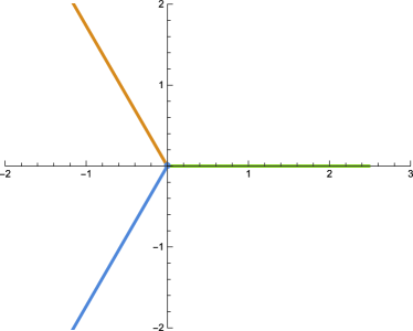
Figure 1: The Stokes lines of the Airy function, which are the solutions of $\mathrm{Im}[s(x)]=0$, are plotted on the complex $x$-plane. The classical turning point of the Schrödinger equation is shown at the origin.

The Stokes lines are the solutions of $\mathrm{Im}[s(x)]=0$.

To understand the Stokes phenomena of the exact WKB analysis, consider the $y$-integration in Eq.(82) for the $\pm$ solutions. Plotting the integration paths on the $y$-plane, one can see that the two paths of the $\pm$ solutions overlap when $x$ is on the Stokes line. (Remember that $\mp s(x)$ is giving the starting point of the $y$-integration and $\mathrm{Im}[s(x)]=0$ is the definition of the Stokes line.) Therefore, one of these solutions (on the left) will develop additional contributions as $x$ goes across the Stokes line. The situation is shown in Fig.2.

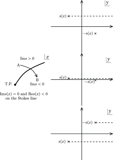
Figure 2: The Stokes phenomenon is explained by the $y$-integration. On the left panel, a Stokes line (the other two are omitted) coming out from a turning point is shown. The Stokes line is drawn on the complex $x$-plane. We take Re$[s(x)]<0$ for the Stokes line. On the right three panels, the contour of the $y$-integration in Eq.(82) is shown. If the solution, whose integration starts from $s(x)$, moves from $A$ to $B$ crossing the Stokes line, the integration contour finally picks up the integration starting from $-s(x)$.

In this case, the solution on the left picks up the other’s integration to give the Stokes phenomenonVirtual:2015HKT . Using the above idea, one can find the connection formulae given by

• Crossing the $\psi_{+}$ Dominant Stokes line with an anticlockwise rotation (seen from the turning point)

  $$\Psi_{+} \rightarrow \Psi_{+}+i\Psi_{-}$$ (84)

  $$\Psi_{-} \rightarrow \Psi_{-}$$ (85)

• Crossing the $\psi_{-}$-Dominant Stokes line with an anticlockwise rotation (seen from the turning point)

  $$\Psi_{-} \rightarrow \Psi_{-}+i\Psi_{+}$$ (86)

  $$\Psi_{+} \rightarrow \Psi_{+}$$ (87)

• An inverse rotation gives a minus sign in front of $i$.

The “dominant” solution in Fig.2 is the one appearing on the left, whose integration contour picks up additional integration after the Stokes phenomenon.

As long as the Stokes lines are not degenerate and no singularities appear, the above connection formulae are versatile. However, in some cases (e.g., scattering due to inverse quadratic potentials), the Stokes lines become degenerate and the above formulae must be reconsidered. The degeneracy can be solved by introducing a small imaginary factor in $\eta$, but the problem is that the formulation becomes discontinuous with respect to the sign of the introduced imaginary factor. The situation is illustrated in Fig.3.

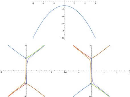
Figure 3: In the upper panel, the potential ($V(x)=-1-x^{2}$) is shown on the $V-x$ plane. In the lower panel, the Stokes lines of $Q(x)=-1-x^{2}\pm 0.05i$ are shown on the complex $x$-planes. One can see that there is a discontinuity between $Q(x)=-1-x^{2}+0.05i$(lower left) and $Q(x)=-1-x^{2}-0.05i$(lower right)

In this case, the normalization factor must be non-trivial to be theoretically consistent with the $\pm$ sign of the imaginary part of $\eta$. The easiest way to find the normalization factor (this factor is called the “Voros coefficient”Voros:1983 ; Delabaere:1993 among mathematicians) is to use consistency relationsBerry:1972na , which is very familiar among physicists. Although the consistency relation cannot give the phase of the normalization factor, it is usually sufficient to discuss cosmological particle productionKofman:1997yn . The exact calculation of the Voros factor is possible in terms of the EWKB, which is calculated in Refs.Voros:1983 ; Delabaere:1993 ; Silverstone:2008 ; Takei:2008 ; Aoki:2009 for the MTP. (The typical example is shown in Fig.3 for the scattering with an inverted quadratic potential.) and a loop structure of a Bessel-like equationAoki:2019 . While we do not always use these exact calculations explicitly, it is important to note that the mathematical proofs always support the calculations in the background.

Since the Stokes phenomena of each MTP structure can be calculated by the EWKB formalismEnomoto:2020xlf ; Enomoto:2021hfv , one can easily obtain the local Bogoliubov transformation occurring at each MTP structure. Using the EWKB, the parameter $\kappa$ (appeared in Sec.1.3 for the Weber function) is given byEnomoto:2020xlf

$$\pi\kappa = \int^{x_{u}}_{x_{d}}S_{odd}dx,$$ (88)

where $x_{u}$ and $x_{d}$ $(Im[x_{u}]>Im[x_{d}])$ are the turning points of the MTP. One might be skeptical about the calculation of the above integral since $S_{odd}$ contains an infinite number of terms. On the complex $t$-plane, the integration can be replaced by a contour integral, which can be calculated very easily for the inverted quadratic potential. Since the EWKB calculation depends only on the Stokes lines and $\kappa$, one can easily calculate the connection matrices of a more complex $Q(x)$ at the MTP structure without referring to the special functions. Indeed, the scattering by a “quartic” potential can be explained by a pair of such MTP structures. (In this case, $\kappa$ of each MTP has to be calculated by the integral of the EWKB.) The situation is shown in Fig.4. We hope the figure helps one understand the importance of the MTP structure. For mathematical details we refer to Ref.Voros:1983 .

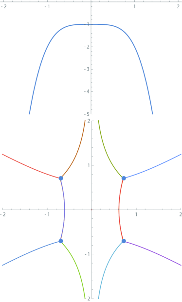
Figure 4: The potential ($V(x)=-1-x^{4}$ on the $V-x$-plane) is shown in the upper panel, and the Stokes lines (for $Q(x)=-1-x^{4}$ on the complex $x$-plane) are shown in the lower panel. One can see two characteristic structures (called “MTP”). The Stokes phenomena (particle production) occur when the real axis of time crosses the Stokes line. In this case, the special function that gives the exact solution is not known. However, from the Stokes lines, one can calculate the connection matrices using the EWKB.

Here is an obvious example where particle production cannot be explained by the MTP structure. Scattering by “tanh”-type potentials gives infinitely degenerate Stokes lines, whose solutions are given by hypergeometric functionsBirrell:1982ix ; Taya:2020dco .

In the case of an inverted quadratic potential, $\kappa$ of the Weber function is identical to the EWKB integral above. In other cases (e.g., the quartic potential in Fig.4), there is no special function that describes the exact solution, so the Stokes phenomenon for the MTP structure must be calculated using integrals.

Since interaction usually raises the order of the differential equation, the problem becomes more complicated than in the original discussion of the Schrödinger-type equation. It should be noted that a complete review of the mathematics behind this analysis is not possible. The analysis of the Stokes phenomena for higher-order differential equations can be found in Refs.Virtual:2015HKT ; Aoki:2019 ; Takei:2008 . To avoid confusion, we will review the EWKB of higher-order differential equations after describing the model setup.

2 Bosonic preheating and the Stokes phenomena

At least one complex scalar field is needed for our discussion of matter-antimatter asymmetry. A closer examination reveals problems with the conventional definition of the creation and annihilation operators in asymptotic states. First, we explain why quantization of a complex scalar field requires special care when introducing CP symmetry breaking.

2.1 Quantization of a real scalar field

The Lagrangian density of a real scalar field is

$${\cal L}=-\frac{1}{2}(\partial_{\mu}\varphi)(\partial^{\mu}\varphi)-\frac{1}{2}m^{2}\varphi^{2}.$$ (89)

The quantization is

$$\varphi(x) = \int\frac{d^{3}\mathbf{k}}{(2\pi)^{3}}\frac{1}{\sqrt{2\omega_{\mathbf{k}}}}\left(a_{\mathbf{k}}e^{-i\omega_{\mathbf{k}}t}+a^{\dagger}_{\mathbf{-k}}e^{i\omega_{\mathbf{k}}t}\right)e^{i\mathbf{kx}}$$

$$= \int\frac{d^{3}\mathbf{k}}{(2\pi)^{3}}\frac{1}{\sqrt{2\omega_{\mathbf{k}}}}\left(a_{\mathbf{k}}e^{i(-\omega_{\mathbf{k}}t+\mathbf{kx})}+a^{\dagger}_{\mathbf{k}}e^{i(\omega_{\mathbf{k}}t-\mathbf{kx})}\right)$$

$$\pi(x) = -i\int\frac{d^{3}\mathbf{k}}{(2\pi)^{3}}\sqrt{\frac{\omega_{\mathbf{k}}}{2}}\left(a_{\mathbf{k}}e^{i(-\omega_{\mathbf{k}}t+\mathbf{kx})}-a^{\dagger}_{\mathbf{k}}e^{i(\omega_{\mathbf{k}}t-\mathbf{kx})}\right),$$

where $\omega_{\mathbf{k}}\equiv\sqrt{\mathbf{k}^{2}+m^{2}}$. Here $\mathbf{x}$ is three-dimensional and $x$ is four-dimensional.

2.2 Quantization of a complex scalar field

A free complex scalar field $\phi$ can be written using two independent real scalar fields $\varphi_{1}$ and $\varphi_{2}$;

$$\phi = \frac{1}{\sqrt{2}}(\varphi_{1}+i\varphi_{2})$$

$$\pi_{\phi} = \frac{\partial{\cal L}}{\partial\dot{\phi}}=\dot{\bar{\phi}}$$ (91)

$$= \frac{1}{\sqrt{2}}(\pi_{\varphi_{1}}-i\pi_{\varphi_{2}})$$

The conventional quantization of the complex scalar field assumes $\omega_{\mathbf{k}}\equiv\omega_{\mathbf{1k}}=\omega_{\mathbf{2k}}$ to define the creation and the annihilation operators as

$$\phi(x) = \int\frac{d^{3}\mathbf{k}}{(2\pi)^{3}}\frac{1}{\sqrt{2\omega_{\mathbf{k}}}}\left(\frac{a_{1\mathbf{k}}+ia_{2\mathbf{k}}}{\sqrt{2}}e^{i(-\omega_{\mathbf{k}}t+\mathbf{kx})}\right.$$

$$\left.+\frac{a^{\dagger}_{1\mathbf{k}}+ia^{\dagger}_{2\mathbf{k}}}{\sqrt{2}}e^{i(\omega_{\mathbf{k}}t-\mathbf{kx})}\right)$$

$$\equiv \int\frac{d^{3}\mathbf{k}}{(2\pi)^{3}}\frac{a_{\mathbf{k}}e^{-ikx}+b^{\dagger}_{\mathbf{k}}e^{ikx}}{\sqrt{2\omega_{\mathbf{k}}}}$$

$$\bar{\phi}(x) = \int\frac{d^{3}\mathbf{k}}{(2\pi)^{3}}\frac{b_{\mathbf{k}}e^{-ikx}+a^{\dagger}_{\mathbf{k}}e^{ikx}}{\sqrt{2\omega_{\mathbf{k}}}}.$$ (92)

where in the last result we have used four-dimensional $k$. In this formalism, the creation and annihilation operators of the complex scalar field are defined by

$$a_{\mathbf{k}} = \frac{a_{1\mathbf{k}}+ia_{2\mathbf{k}}}{\sqrt{2}}$$

$$b_{\mathbf{k}} = \frac{a_{1\mathbf{k}}-ia_{2\mathbf{k}}}{\sqrt{2}}.$$ (93)

The above definitions are used to define asymptotic states. We will see why these definitions are causing trouble in our case.

Let us first examine the validity of the primary assumption $\omega_{\mathbf{1k}}=\omega_{\mathbf{2k}}$. To define the matter and the antimatter states for the asymptotic states, we consider the case in which CP-violating interactions vanish at $t=\pm\infty$. The above definitions of the creation and the annihilation operators are valid in those limits. On the other hand, due to the CP-violating interaction, the above states could be mixed during preheating, and there is no reason to believe in $\omega_{\mathbf{1k}}=\omega_{\mathbf{2k}}$.

To see what happens, we introduce the simplest term of CP violation as

$${\cal L}_{CP} = \frac{1}{2}\left[\Lambda(t)\phi^{2}+h.c\right]$$ (94)

$$= \frac{1}{2}\left[\Lambda(\varphi_{1}^{2}-\varphi_{2}^{2}+2i\varphi_{1}\varphi_{2})+\Lambda^{*}(\varphi_{1}^{2}-\varphi_{2}^{2}-2i\varphi_{1}\varphi_{2})\right]$$

$$= \Lambda_{R}(\varphi_{1}^{2}-\varphi_{2}^{2})-2\Lambda_{I}\varphi_{1}\varphi_{2},$$

where we defined $\Lambda=\Lambda_{R}+i\Lambda_{I}$. Now we consider a situation where $\Lambda_{R}$ is a constant and the function $\Lambda_{I}(t)$ can be regarded as a perturbation parameter. Expanding $\varphi_{i}=\varphi_{i(0)}+\varphi_{i(1)}+...$, the perturbative calculation with the time-dependent interaction $\Lambda_{I}(t)$ gives

$$(\partial_{t}+\mathbf{k}^{2}+m_{\phi}^{2}-2\Lambda_{R})\varphi_{1(1)} = \Lambda_{I}(t)\varphi_{2(0)}$$ (95)

$$= \Lambda_{I}(t)e^{-i\omega_{\mathbf{2}}t},$$

where (because of ${\cal L}_{CP}$)

$$\omega_{1} = \sqrt{\mathbf{k}^{2}+m_{\phi}^{2}-2\Lambda_{R}}$$

$$\omega_{2} = \sqrt{\mathbf{k}^{2}+m_{\phi}^{2}+2\Lambda_{R}}.$$ (96)

Here the subscript $\mathbf{k}$ is omitted for simplicity. Using the Green function and defining the Fourier transformation of $\Lambda_{I}(t)$ by $\tilde{\Lambda}_{I}(\omega)$, we have

$$\varphi_{1(1)}=-\int\frac{d\omega^{\prime}}{2\pi}\frac{\tilde{\Lambda}_{I}(\omega^{\prime}-\omega_{2})}{(\omega^{\prime})^{2}-(\mathbf{k}+m_{\phi}^{2}-2\Lambda_{R})}e^{-i\omega^{\prime}t}.$$ (97)

Considering the residues at $\omega^{\prime}=-\omega_{1}$, we find the coefficient of $e^{+i\omega_{1}t}$ to be

$$\beta_{1,\mathbf{k}}=i\frac{\tilde{\Lambda}_{I}^{*}(\omega_{1}+\omega_{2})}{2\omega_{1}}.$$ (98)

The above calculation is almost the same as the calculation of Ref.Dolgov:1996qq except for the quantization, which is crucial in our case. Because of the different signs in front of $\varphi_{1}^{2}$ and $\varphi_{2}^{2}$ in Eq.(94), we have $\omega_{1}\neq\omega_{2}$. This discriminates $\beta_{\mathbf{1k}}$ and $\beta_{\mathbf{2k}}$, and could be a crucial source of the asymmetry (the mechanism of the asymmetry generation is not trivial, as we will see below). What we consider in this paper is the CP-violating interaction, which introduces intermediate states of $\omega_{1}\neq\omega_{2}$.

One can write the mass matrix and the CP-violating interactions in a matrix form

$$M = \left(\begin{array}[]{cc}m_{\phi}^{2}&\Lambda^{*}\\ \Lambda&m_{\phi}^{2}\end{array}\right),$$ (101)

which normally gives the higher-order differential equations after decoupling. Note however the matrix can be diagonalized and the equations become the second-order differential equations if all elements are constant. Using the formalism of the exact WKB for the higher-order differential equations, we are going to find the source of asymmetry in this model.

2.3 Case1: Real $\Lambda(t)$

Let us first assume that $\Lambda(t)$ is a real function. Using Eq.(94) and $\Lambda_{I}=0$, the interaction between $\varphi_{1}$ and $\varphi_{2}$ vanishes, and the equations of $\varphi_{1},\varphi_{2}$ are separated. In this case, we do not have to consider the higher-order differential equations. On the other hand, their masses are distinguished as

$$m_{1}^{2} = m_{\phi}^{2}-2\Lambda_{R}$$

$$m_{2}^{2} = m_{\phi}^{2}+2\Lambda_{R}.$$ (102)

For the real $\Lambda(t)$, $\varphi_{1}$ and $\varphi_{2}$ are independent and are not equal. The Stokes phenomenon occurs independently and does not mix the asymptotic solutions of $\varphi_{1}$ and $\varphi_{2}$. Our question is whether the asymmetry production is possible or not in this case. To be more precise, we are going to identify the Stokes phenomena, which is responsible for the matter-antimatter asymmetry. What we can assume here is just $\beta_{\mathbf{11k}}\neq\beta_{\mathbf{22k}}$ and $\beta_{\mathbf{12k}}=\beta_{\mathbf{21k}}=0$. (The subscripts $\mathbf{12k}$ and $\mathbf{21k}$ denote the mixing of solutions between $\varphi_{1}$ and $\varphi_{2}$.) Does this difference source the matter-antimatter asymmetry in the asymptotic states? To understand the situation, we will write the Bogoliubov transformation of the original creation and annihilation operators in a matrix form and translate it to the asymptotic states. For the relation between the asymptotic states of Eq.(2.2) and the original creation and annihilation operators of $\varphi_{1}$ and $\varphi_{2}$, we define in the limit $t=-\infty$ as

$$\left(\begin{array}[]{c}a_{\mathbf{k}}\\ a^{\dagger}_{\mathbf{k}}\\ b_{\mathbf{k}}\\ b^{\dagger}_{\mathbf{k}}\end{array}\right) = \frac{1}{\sqrt{2}}\left(\begin{array}[]{cccc}1&0&i&0\\ 0&1&0&-i\\ 1&0&-i&0\\ 0&1&0&i\end{array}\right)\left(\begin{array}[]{c}a_{1\mathbf{k}}\\ a^{\dagger}_{1\mathbf{k}}\\ a_{2\mathbf{k}}\\ a^{\dagger}_{2\mathbf{k}}\end{array}\right).$$ (115)

We can write the Bogoliubov transformations of the original operators in the following form;

$$\left(\begin{array}[]{c}a_{1\mathbf{k}}\\ a^{\dagger}_{1\mathbf{k}}\\ a_{2\mathbf{k}}\\ a^{\dagger}_{2\mathbf{k}}\end{array}\right)^{\prime} = \left(\begin{array}[]{cccc}\alpha_{\mathbf{11k}}&\beta_{\mathbf{11k}}&0&0\\ \beta^{*}_{\mathbf{11k}}&\alpha^{*}_{\mathbf{11k}}&0&0\\ 0&0&\alpha_{\mathbf{22k}}&\beta_{\mathbf{22k}}\\ 0&0&\beta^{*}_{\mathbf{22k}}&\alpha^{*}_{\mathbf{22k}}\\ \end{array}\right)\left(\begin{array}[]{c}a_{1\mathbf{k}}\\ a^{\dagger}_{1\mathbf{k}}\\ a_{2\mathbf{k}}\\ a^{\dagger}_{2\mathbf{k}}\end{array}\right)$$ (128)

Using Eq.(115) and Eq.(128), the Bogoliubov transformations of the asymptotic states are given by

$$a_{\mathbf{k}} \rightarrow \frac{1}{\sqrt{2}}\left(\alpha_{\mathbf{11k}}a_{\mathbf{1k}}+i\alpha_{\mathbf{22k}}a_{\mathbf{1k}}+\beta_{\mathbf{11k}}a^{\dagger}_{\mathbf{1k}}+i\beta_{\mathbf{22k}}a^{\dagger}_{\mathbf{2k}}\right)$$

$$b_{\mathbf{k}} \rightarrow \frac{1}{\sqrt{2}}\left(\alpha_{\mathbf{11k}}a_{\mathbf{1k}}-i\alpha_{\mathbf{22k}}a_{\mathbf{1k}}+\beta_{\mathbf{11k}}a^{\dagger}_{\mathbf{1k}}-i\beta_{\mathbf{22k}}a^{\dagger}_{\mathbf{2k}}\right),$$ (130)

which give

$$n=\bar{n} = \frac{|\beta_{\mathbf{11k}}|^{2}+|\beta_{\mathbf{22k}}|^{2}}{2}.$$ (131)

Therefore, despite the difference between $\varphi_{1}$ and $\varphi_{2}$, asymmetry production is impossible for real $\Lambda(t)$. A possible source of the asymmetry is the contribution from the off-diagonal blocks ($\alpha_{\mathbf{12k}}$ and $\beta_{\mathbf{12k}}$, which are $0$ in Eq.(128)), which could introduce the asymmetry as $|\beta_{\mathbf{11k}}+i\beta_{\mathbf{12k}}|^{2}\neq|\beta_{\mathbf{11k}}-i\beta_{\mathbf{12k}}|^{2}$. This is nothing but a quantum interference between different Stokes phenomena. However, the off-diagonal blocks always vanish for the real $\Lambda(t)$. We are going to examine this possibility in the next section.

2.4 Case2: Complex $\Lambda(t)$

We have learned that the Stokes phenomena, which do not mix $\varphi_{1}$ and $\varphi_{2}$, cannot generate the required asymmetry even though $\varphi_{1}$ and $\varphi_{2}$ are distinguishable. The asymmetry can be generated if the interference $|\beta_{\mathbf{11k}}+i\beta_{\mathbf{12k}}|^{2}\neq|\beta_{\mathbf{11k}}-i\beta_{\mathbf{12k}}|^{2}$ is possible, but what process is responsible for the off-diagonal blocks in the matrix of Eq.(128)?

To generate the interference, the Stokes phenomenon has to happen at least twice. They are $\beta_{\mathbf{11k}}$ or $\beta_{\mathbf{22k}}$ ($\varphi_{1}$ and $\varphi_{2}$ are not mixed) and $\beta_{\mathbf{12k}}$(mixed). Therefore, we need a higher-order differential equation to realize the Stokes phenomena. Since the higher-order differential equation is very complicated, we are going to pick up the essentials and explain how to introduce the asymmetry in physics.

3 The EWKB for the higher-order differential equations

In this section, we discuss the Stokes phenomena for a complex scalar field with a CP-violating interaction. We begin with the simple cases of second and third-order differential equations to illuminate the Stokes phenomena of the higher-order differential equations. Finally, we show the local structure of the Stokes lines that cause the asymmetry.

3.1 From the first-order simultaneous differential equation to the Schrödinger equation

Before discussing the simultaneous second-order differential equation with a $2\times 2$ matrix, let us first discuss a simultaneous first-order differential equation with a $2\times 2$ matrix. The point of discussion is the relationship between the conventional Schrödinger-like equation (where the solutions are given by simple $\pm$ solutions) and the formulation given by $\zeta$. (What $\zeta$ is will be explained in this section.)

In cosmology, a simultaneous first-order differential equation with a $2\times 2$ matrix is found in the dynamical particle production of Majorana fermions, which is very similar to the Landau-Zener model. (The Landau-Zener model is normally discussed for constant off-diagonal elements. See Appendix A for more details.) Following Refs.Enomoto:2020xlf ; Enomoto:2021hfv , we start with

$$i\hbar\frac{d}{dt}\left(\begin{array}[]{c}X\\ Y\end{array}\right) = \left(\begin{array}[]{cc}D(t)&\Delta(t)^{*}\\ \Delta(t)&-D(t)\end{array}\right)\left(\begin{array}[]{c}X\\ Y\end{array}\right),$$ (138)

which can be decoupled to give

$$\hbar^{2}\ddot{X}-\hbar\frac{\dot{\Delta}^{*}}{\Delta^{*}}\dot{X}+\left(-\frac{i\hbar D\dot{\Delta}^{*}}{\Delta^{*}}+i\hbar\dot{D}+|\Delta|^{2}+D^{2}\right)X=0.$$

We introduce $p_{1}(\hbar,t)$ and $p_{0}(\hbar,t)$ to rewrite the equation in the following form:

$$\ddot{X}+\frac{p_{1}(\hbar,t)}{\hbar}\dot{X}+\frac{p_{0}(\hbar,t)}{\hbar^{2}}X = 0.$$ (140)

The “Schrödinger equation” can be recovered by using the transformation

$$X = \exp\left(-\frac{1}{2}\int^{x}\frac{p_{1}}{\hbar}dx\right)\hat{X}$$ (141)

Finally, we have the second-order ordinary equation of the Schrödinger-type;

$$\hbar^{2}\ddot{\hat{X}} + \left(p_{0}-\frac{p_{1}^{2}}{4}-\frac{\hbar}{2}p_{1}^{\prime}\right)\hat{X}=0.$$ (142)

Applying the EWKB, $\hat{S}_{-1}$ becomes

$$\hat{S}_{-1}^{2} = -\left(|\Delta|^{2}+D^{2}\right)+\frac{(\dot{\Delta})^{2}}{4(\Delta)^{2}},$$ (143)

which gives the $\pm$-solutions.

In the above calculation, we have introduced a non-trivial transformation to find the Schrödinger-type equation. Alternatively, for the original $X$ of Eq.(140), one may calculate

$$S_{-1}^{2}+p^{(0)}_{1}(t)S_{-1}+p^{(0)}_{0}(t) = 0,$$ (144)

where $p_{i}^{(n)}$ is the coefficient of $\hbar^{n}$ when $p_{i}$ is expanded by $\hbar$. For $S_{-1}$ of the original equation, we have two solutions

$$\zeta_{\pm} = -\frac{p_{1}^{(0)}\pm\sqrt{(p_{1}^{(0)})^{2}-4p_{0}^{(0)}}}{2},$$ (145)

which define the “turning points” at the solutions of $\zeta_{+}=\zeta_{-}$. In this case, the Stokes lines are defined by

$$\mathrm{Im}\left[\int_{a}^{t}(\zeta_{+}-\zeta_{-})dt\right] = 0,$$ (146)

where the constant $a$ normally denotes the turning point from which the Stokes lines are coming out.

The above formulation of $\zeta_{\pm}$ is more general than the formulation based on the Schrödinger-type equation. It is easy to see that the $\zeta$-formalism is essential to the EWKB for higher-order differential equations. Also, when applied to the Landau-Zener transition at “level crossings”, the $\zeta$-formalism is much more intuitive than the Schrödinger-type formalism.

From the above discussion, it is easily understood that Schrödinger-type equations can be reformed from $\zeta_{\pm}$. Although not accurate, (see Ref.Virtual:2015HKT for more accurate discussions) such reconstruction is also locally possible near a turning point defined for a pair of solutions of higher-order differential equations. Since in physics of particle creation the Stokes phenomenon (which is defined for a pair of solutions) occurs when the real axis crosses the Stokes line, the Schrödinger-type equation reconstructed from the pair is responsible for the connection matrix of the particle creation at that moment. Also, if the linear approximation is possible for the “level crossings”, the Stokes lines are locally given by the MTP. (See appendix A for the “linear approximation” used in the original Landau-Zener model.) Since the Stokes phenomena of the MTP structure is calculable, the connection matrix for such a general case can be calculated. Therefore, although the mathematics of higher-order differential equations is theoretically very complex, by decomposing the essential elements into familiar MTP structures, one can find how the physics can be embedded. This is the basic strategy of this paper.

In the next section, we analyze two typical third-order differential equations in which the new Stokes line appears.

3.2 The “new Stokes lines” of the third-order equation

Let us extend the EWKB analysis and the formulation of the previous section to the third-order ordinary differential equation. We consider the model given by Berk, Nevis, and Roberts(NBR)NBR , which is defined by

$$\left[\frac{d^{3}}{dt^{3}}+3\eta^{2}\frac{d}{dt}+2it\eta^{3}\right]\psi(t) = 0,$$ (147)

where $\eta\equiv\hbar^{-1}$ is a large parameter for the WKB expansion. $S_{-1}$ obeys the equation given by

$$\zeta^{3}+3\zeta+2it = 0,$$ (148)

which has solutions

$$\zeta_{1} = -\frac{1}{\left(-it+\sqrt{1-t^{2}}\right)^{\frac{1}{3}}}+\left(-it+\sqrt{1-t^{2}}\right)^{\frac{1}{3}}$$

$$\zeta_{2} = \frac{1+i\sqrt{3}}{2\left(\sqrt{1-t^{2}}-it\right)^{\frac{1}{3}}}-\frac{1}{2}\left(1-i\sqrt{3}\right)\left(\sqrt{1-t^{2}}-it\right)^{\frac{1}{3}}$$

$$\zeta_{3} = \frac{1-i\sqrt{3}}{2\left(\sqrt{1-t^{2}}-it\right)^{\frac{1}{3}}}-\frac{1}{2}\left(1+i\sqrt{3}\right)\left(\sqrt{1-t^{2}}-it\right)^{\frac{1}{3}}.$$

The formal turning points are $t=-1$ for $\zeta_{1}=\zeta_{2}$ and $t=1$ for $\zeta_{1}=\zeta_{3}$, both of which are the Airy-type (i.e, three Stokes lines are coming out of a turning point). The Stokes lines are presented in Fig.5.

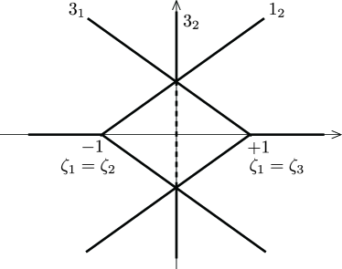
Figure 5: Each Stokes lines are for a pair of two solutions. The numberings are denoting the two solutions. For $3_{1}$, the dominant solution is “$3$”, and the Stokes phenomena occurs for “$3$” and “$1$”. The line denoted by $3_{2}$ is the “new Stokes line”, but the dotted part does not cause the Stokes phenomena.

Without the “new Stokes line” denoted by $3_{2}$ in Fig.5, the connection formulae are inconsistent between the route above and below the crossing points of $1_{2}$ and $3_{1}$. (Details of the calculation are given in Ref.NBR . Without the New Stokes line, the connection matrix seems to depend on the route.) The new Stokes line ($3_{2}$) was introduced to solve the problem of the global inconsistency. Note that the Stokes phenomenon is not observed on the dotted part. (This was the speculation in Ref.NBR , but later worksAoki:2019 ; Takei:2008 ; Virtual:2015HKT revealed the mathematics behind it.) The regular and the dotted parts of the new Stokes line are easily distinguished by considering the consistency of the Stokes phenomena around the crossing points.

Using the EWKB, one can find an extra turning point at the origin, which was named the “virtual turning point”Virtual:2015HKT . The virtual turning point is the solution of

$$\int^{t_{v}}_{t_{12}}(\zeta_{2}-\zeta_{1})dt = \int^{t_{v}}_{t_{13}}(\zeta_{3}-\zeta_{1})dt.$$ (150)

Here $t_{ij}$ is the solution of $\zeta_{i}=\zeta_{j}$ (normal turning points), which are $t_{12}=-1$ and $t_{13}=1$ in this case. One can solve the equation to find the virtual turning point at $t_{v}=0$. Since the virtual turning point is placed on the dotted line, it causes nothing in physics (but is very important in mathematics).

In the above example of the NBR equation, there were two Airy-type turning points on the real axis. Although the NBR model is very informative and historically important for understanding the new Stokes lines, it does not describe the scattering problem in physics. Therefore, we will consider another model in which the Stokes lines have local MTP structures. Following Ref.Virtual:2015HKT , we consider a three-level Landau-Zener modelZener:1932ws . In the multi-level Landau-Zener model, the MTP structure appears at each level crossing. In the three-level Landau-Zener model, there are three kinds of MTP for level crossings because level crossings are defined for pairs.

The model is described by

$$i\frac{d}{dt}\psi = \eta H(t,\eta)\psi$$ (151)

with

$$H(t,\eta) = H_{0}(t)+\eta^{-\frac{1}{2}}H_{\frac{1}{2}}$$

$$H_{0}(t) = \left(\begin{array}[]{ccc}\rho_{1}(t)&0&0\\ 0&\rho_{2}(t)&0\\ 0&0&\rho_{3}(t)\end{array}\right)$$ (155)

$$= \left(\begin{array}[]{ccc}t+3&0&0\\ 0&2t&0\\ 0&0&4t\end{array}\right)$$ (159)

$$H_{\frac{1}{2}} = \left(\begin{array}[]{ccc}0&c_{12}&c_{13}\\ \bar{c}_{12}&0&c_{23}\\ \bar{c}_{13}&\bar{c}_{23}&0\end{array}\right).$$ (163)

After decoupling, $S_{-1}$ obeys the equation

$$\zeta^{3}+i(7t+3)\zeta^{2}-2t(7t+9)\zeta-8it^{2}(t+3) = 0,$$ (164)

which has three solutions given by

$$\zeta_{1}= i(t+3) =i\rho_{1}(t)$$

$$\zeta_{2}= i2t =i\rho_{2}(t)$$

$$\zeta_{3}= i4t =i\rho_{3}(t).$$ (165)

The turning points are

$$\zeta_{2}=\zeta_{3} \rightarrow t_{23}=0$$

$$\zeta_{1}=\zeta_{3} \rightarrow t_{13}=1$$

$$\zeta_{1}=\zeta_{2} \rightarrow t_{12}=3,$$ (166)

where $t_{23}<t_{13}<t_{12}$.

From this result, one will understand how the off-diagonal elements of the above model simplify the argument. Because of the factor $\eta^{-\frac{1}{2}}$ in front of $H_{\frac{1}{2}}$, elements ($c_{ij}$) disappear from $\zeta_{i}$. Although extra $\hbar$ could not be acceptable in physics, this factor mimics small interaction and was introduced to make the model instructive. In this model, the MTP structure of the Landau-Zener model is the double turning point, from which the four Stokes lines extend.

In this model, turning points are found at $t=0,1,3$ and the structure of the Stokes lines is very simple, as is shown in Fig.6. One can see “ordered crossing points”(a new Stokes line is needed) and “non-ordered crossing points”(a new Stokes line is not needed) in Fig.6. To understand the “consistency” required for the Stokes lines, one can explicitly write down the connection matrices of the Stokes phenomena. At the crossing point of $1_{2}$ and $3_{2}$, the Stokes phenomena do not depend on the route because the matrices $U_{1_{2}}$ and $U_{3_{2}}$ commute, while at the crossing point of $1_{3}$ and $3_{2}$, the matrices $U_{1_{3}}$ and $U_{3_{2}}$ do not commute. To make the Stokes phenomena route-independent, one has to introduce another stokes line at the crossing point of $1_{3}$ and $3_{2}$. Of course, the mathematics behind this phenomenon is not so trivial. More details and rigorous arguments are described in Ref.Virtual:2015HKT .

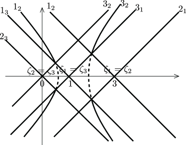
Figure 6: Unlike the NBR model, each level crossing gives the (degenerated) MTP structure, from which four Stokes lines are coming out.

3.3 The EWKB for a complex scalar field with CP violation

Finally, we are going to solve the equations for the real scalar fields $\varphi_{1,2}$ of the complex scalar $\phi$. We write

$$-\hbar^{2}\frac{d^{2}}{dt^{2}}\left(\begin{array}[]{c}\varphi_{1}\\ \varphi_{2}\end{array}\right) = \Omega(t)\left(\begin{array}[]{c}\varphi_{1}\\ \varphi_{2}\end{array}\right),$$ (171)

where the matrix $\Omega(t)$ is given by

$$\Omega(t) = \left(\begin{array}[]{cc}D_{1}&\Delta\\ \Delta&D_{2}\end{array}\right)$$ (174)

$$= \left(\begin{array}[]{cc}\omega_{\mathbf{k1}}^{2}-2\Lambda_{R}&2\Lambda_{I}\\ 2\Lambda_{I}&\omega_{\mathbf{k2}}^{2}+2\Lambda_{R}\end{array}\right).$$ (177)

After separating $\Lambda(t)=\Lambda_{R}+i\Lambda_{I}$, all elements of the matrix are real. Defining

$$\varphi_{1}^{(i)}\equiv\frac{d^{i}}{dt^{i}}\varphi_{1},$$ (178)

the decoupled equations (the 4th-order ordinary differential equations) can be written as

$$\sum_{i=0}^{4}p_{i}\varphi_{1}^{(i)} = p_{4}\varphi_{1}^{(4)}+p_{3}\varphi_{1}^{(3)}+p_{2}\varphi_{1}^{(2)}+p_{1}\varphi_{1}^{(1)}+p_{0}\varphi_{1}$$ (179)

$$= 0.$$

Coefficients are given by

$$\frac{p_{4}}{\hbar^{4}} = 1$$

$$\frac{p_{3}}{\hbar^{3}} = -2\hbar\frac{\Delta^{\prime}}{\Delta}$$

$$\frac{p_{2}}{\hbar^{2}} = D_{1}+D_{2}+\hbar^{2}\left[\frac{2(\Delta^{\prime})^{2}-\Delta\Delta^{\prime\prime}}{\Delta^{2}}\right]$$

$$\frac{p_{1}}{\hbar} = 2\hbar\frac{-D_{1}\Delta^{\prime}+\Delta D_{1}^{\prime}}{\Delta}$$

$$p_{0} = -\Delta^{2}+D_{1}D_{2}+\hbar^{2}\left[-\frac{2\Delta^{\prime}D_{1}^{\prime}-2D_{1}(\Delta^{\prime})^{2}}{\Delta}+D_{1}^{\prime\prime}-D_{1}\Delta^{\prime\prime}\right].$$

Assuming that time-dependent background fields are all external, we have

$$\zeta^{4}+2(D_{1}+D_{2})\zeta^{2}+D_{1}D_{2}-\Delta^{2} = 0,$$ (181)

which has four solutions given by

$$\zeta_{A\pm} \equiv \pm\frac{\sqrt{-(D_{1}+D_{2})+\sqrt{4\Delta^{2}+(D_{1}-D_{2})^{2}}}}{\sqrt{2}}$$

$$= \pm\frac{\sqrt{-(\omega_{\mathbf{k1}}^{2}+\omega_{\mathbf{k2}}^{2})+4\sqrt{\Lambda_{I}^{2}+\Lambda_{R}^{2}}}}{\sqrt{2}}$$

$$\zeta_{B\pm} \equiv \pm\frac{\sqrt{-(D_{1}+D_{2})-\sqrt{4\Delta^{2}+(D_{1}-D_{2})^{2}}}}{\sqrt{2}}$$ (182)

$$= \pm\frac{\sqrt{-(\omega_{\mathbf{k1}}^{2}+\omega_{\mathbf{k2}}^{2})-4\sqrt{\Lambda_{I}^{2}+\Lambda_{R}^{2}}}}{\sqrt{2}}.$$

Here $\pm$-pair solutions correspond to asymptotic $\pm$-solutions of real scalar fields ($\varphi_{1,2}$).

Let us assume that $m_{\phi}(t),\Lambda_{R}(t),\Lambda_{I}(t)$ are all independent and time-dependent. (Although the original $m_{\phi}(t),\Lambda_{R}(t),\Lambda_{I}(t)$ are defined to be real, they are complex on the complex $t$-plane.) The turning points are given by

1. $\zeta_{A+}-\zeta_{A-}=0$ ($\zeta_{A\pm}=0$);

   $$D_{1}+D_{2} = \sqrt{\Lambda_{R}^{2}+\Lambda_{I}^{2}}$$ (183)

2. $\zeta_{B+}-\zeta_{B-}=0$ ($\zeta_{B\pm}=0$);

   $$D_{1}+D_{2} = -\sqrt{\Lambda_{R}^{2}+\Lambda_{I}^{2}}$$ (184)

3. $\zeta_{A\pm}-\zeta_{B\pm}=0$;

   $$\Lambda_{R}^{2}+\Lambda_{I}^{2} = 0,$$ (185)

4. $\zeta_{A\pm}-\zeta_{B\mp}=0$;

   $$\Lambda_{R}^{2}+\Lambda_{I}^{2}=0 D_{1}+D_{2}=0.$$ , (186)

The MTP of the last turning points (4.) is expected to generate $\beta_{\mathbf{12k}}$ by itself. However, they can be ignored in physics because the two conditions must be satisfied simultaneously. The required $\beta_{\mathbf{12k}}\neq 0$ will be generated by the combinations of the Stokes phenomena of the other turning points. In this section, we will denote the above turning points (1., 2. and 3.) by the numbers given above.

In addition, one can see that if the interaction is given by $\Lambda(t)=\Lambda_{0}e^{i\theta(t)}$, it gives

$$\Lambda_{I}^{2}+\Lambda_{R}^{2}=\Lambda_{0}^{2},$$ (187)

which extinguishes the required turning points (3.) from the scenario. Therefore, the asymmetry production is theoretically impossible for $\Lambda(t)=\Lambda_{0}e^{i\theta(t)}$. On the other hand, one might be tempted to expand it for $\theta(t)=A\cos\omega_{I}t,A\ll 1$ as

$$\Lambda(t) = \Lambda_{0}e^{i\theta(t)}$$ (188)

$$\simeq \Lambda_{0}\left[1+i\theta(t)\right]$$

$$= \Lambda_{0}\left[1+iA\cos\omega_{I}t\right],$$

which can generate false turning points (3.) on the complex $t$-plane. Note that the above expansion is nothing but the expansion considered in Ref.Dolgov:1996qq for baryogenesis after natural inflation. The above simple calculation shows why naive expansions are dangerous in non-perturbative analysis.

To understand the required structure of the Stokes lines, we show the simplest Stokes lines in Fig.7, for which fig.6 is extended to the four-level Landau-Zener transition. (Here we have four solutions $\zeta_{A\pm}$ and $\zeta_{B\pm}$.) For illustration, turning points are manually aligned, and are shown to have degenerated MTP structure (i.e, the off-diagonal elements of the local Landau-Zener transition are supposed to be small). What we are considering here is a simple situation in which the interference between the Stokes phenomena is possible. If the particle production is caused by oscillation, there should be many turning points (MTP) in the global structure. One can easily construct many exceptional cases (e.g, using tanh to make the Stokes lines infinitely degenerated, or introducing singularities).

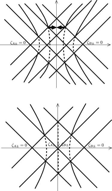
Figure 7: The turning point of 3. is placed between the two (1. and 2.) turning points. In the upper panel, the degenerated turning points of 3. are manually separated for illustration. For simplicity, each turning point is shown by a double turning point of a pair of MTP. In the lower panel, mixing between $A$ and $B$ occurs near the origin.

Since the Stokes lines emanating from turning points 1. and 2 do not have a common solution, their intersection obviously does not require a new Stokes line. On the other hand, the Stokes lines from the turning point 3. have a common solution with the Stokes lines from 1. and 2., which means that new Stokes lines may emerge from the intersection.

Fig.7 shows that the new Stokes lines are all drawn as dotted lines when they intersect the real axis, with no extra influence. If the motion of the time-dependent parameters is oscillatory, the MTP structures of the turning points 1.2. and 3. may appear repeatedly. However, seeing the Stokes lines of the simplest case, one would expect that changing the ordering of the turning points will not drastically change the situation. To avoid confusion, we confess that “unfortunately” we could not find out a way to include such effects in physics. The “extra” contribution from the new Stokes lines, if it had contributed, could have introduced the desired interference in a new way. We failed to include the new Stokes lines in physics, but our conclusion is far from a no-go theorem. Higher-order differential equations are very complex, and what we have shown in this paper should be only a small part of the whole. Indeed, for the model considered in Ref.Shudo:2020 , it was found that the new Stokes line comes into play. Also, the assumption that the MTP structures are responsible for particle production (this corresponds to the conventional linear approximation of the Landau-Zener model) makes our arguments very simple. What we have shown is that just one MTP of the turning point (3.) appearing among other turning points can generate matter-antimatter asymmetry.

We have shown that interference between different Stokes phenomena is essential for the asymmetry. In order for interference to occur, there must be a mixture of Stokes phenomena with $\varphi_{1}$ solutions and $\varphi_{2}$ solutions. This criterion is the main result of this paper. As far as we know, this is the first paper to point out the importance of the interference between different Stokes phenomena for the asymmetry of dynamical particle production.

Although the model examined in this paper is very simple, in which only a complex scalar field and the simplest interaction are considered, we believe that the model has the essential properties of dynamical particle production with CP-violating interactions and is giving the first example of the analysis in which the interference between different Stokes phenomena is taken into account for the higher-order differential equation.

4 Conclusions and discussions

In this paper, we have analyzed the mechanism of matter-antimatter asymmetry generation during preheating when CP is broken. We found that interference between different Stokes phenomena is an important factor in asymmetry generation. This criterion is the main result of this paper. To the best of our knowledge, this is the first paper to point out that interference between different Stokes phenomena is crucial for the asymmetry in dynamical particle production. Although the model considered in this paper is very simple, we believe it has the essential properties of dynamical particle production with CP-violating interactions.

In our analysis, the quantization given by Eq.(2.2) does not hold for the transition process. Therefore, we discussed particle generation using the original creation and annihilation operators of the real fields $\varphi_{1}$ and $\varphi_{2}$. What makes the analysis difficult is the fourth-order differential equation that appears after decoupling the simultaneous differential equations. This equation is so complex that we had to carefully pick out the essential elements that describe the physics. We followed the analysis of the multi-level Landau-Zener model.

The EWKB analysis considers the Borel resummation, and its Stokes lines describe the global structure (i.e, the connection formulae). Higher-order differential equations require new Stokes lines and virtual turning points for global consistency. The key questions for physics are (1) what Stokes phenomena are responsible for (asymmetric) particle production, and (2) whether the “new” objects in the higher-order differential equation are changing the traditional particle production scenario. We then identified the Stokes phenomena responsible for the asymmetry. The matter-antimatter asymmetry requires mixing between the asymptotic solutions of $\varphi_{1}$ and $\varphi_{2}$, which is possible only when $\Lambda_{I}$ exists. For our calculations, we had to draw a structure of the Stokes lines in order to understand which Stokes lines are responsible for the Bogoliubov transformation of the model. Unfortunately, at least in the simple model considered in this paper, all new Stokes lines are drawn as dotted lines on the real-time axis and play no significant role in physics.

We have used the idea that the situation near particle production is similar to the Landau-Zener transition; the MTP gives a simple connection matrix, which is a simple and straightforward way to calculate the local system. The basic calculations for the local system are similar to the conventional preheating scenario or the Landau-Zener transition.

As a by-product, we have proven that a rotational motion, which is given by $\Lambda(t)=\Lambda_{0}e^{i\theta(t)}$ or $\Lambda(t)=\Lambda_{0}e^{iA\cos(\omega t)}$, cannot generate matter-antimatter asymmetry in this model. This tells us that expanding the interaction as $\Lambda_{0}e^{iA\cos(\omega t)}\simeq\Lambda_{0}[1+iA\cos(\omega t)]$ for small $A$ is very dangerous. In light of the EWKB, such a perturbative expansion can easily change the global structure of the Stokes lines, generating false turning points on the complex $t$-plane.

Finally, we will compare our present result with our earlier calculation of asymmetric preheatingEnomoto:2021hfv . In our previous calculation, we had considered time-dependent off-diagonal elements of the simultaneous differential equation of a Majorana fermion to find that the helicity asymmetry occurs when particle production is not simultaneous between different helicity states. After decoupling, the equation of a Majorana fermion is the second-order differential equation and there is no interference of the Stokes phenomena between different species. In this paper, we have shown that the interference of the Stokes phenomenon is the essence of asymmetry for a certain model, but we do not rule out other possibilities for the asymmetry generation.

Appendix A The Stokes phenomena for the Landau-Zener transition

We show how the Landau-Zener modelZener:1932ws can be related to the Stokes phenomena of cosmological particle production. The point is that the Stokes lines of the Landau-Zener transition give the MTP structure at the transition, where the “level crossing” occurs. For the extended Landau-Zener model with multiple levels, the MTP structure appears at each level crossing.

We introduce the “velocity” $v>0$ and the off-diagonal elements $\Delta$, both of which are supposed to be real. The Landau-Zener model uses a couple of ordinary differential equations given by

$$i\hbar\frac{d}{dt}\left(\begin{array}[]{c}\psi_{1}\\ \psi_{2}\end{array}\right) = \left(\begin{array}[]{cc}-\frac{v}{2}t&\Delta\\ \Delta&+\frac{v}{2}t\end{array}\right)\left(\begin{array}[]{c}\psi_{1}\\ \psi_{2}\end{array}\right),$$ (195)

which can be decoupled to give

$$\left[\hbar^{2}\frac{d^{2}}{dt^{2}}+\left(\Delta^{2}-i\hbar\frac{v}{2}\right)+\frac{1}{4}v^{2}t^{2}\right]\psi_{1} = 0$$ (196)

$$\left[\hbar^{2}\frac{d^{2}}{dt^{2}}+\left(\Delta^{2}+i\hbar\frac{v}{2}\right)+\frac{1}{4}v^{2}t^{2}\right]\psi_{2} = 0.$$ (197)

Following Refs.Virtual:2015HKT ; Voros:1983 ; Delabaere:1993 ; Silverstone:2008 , we are going to rewrite the equations in the standard EWKB form. We have

$$\left[-\frac{d^{2}}{dx^{2}}+\eta^{2}Q(x)\right]\psi(x,\eta) = 0,$$ (198)

where

$$Q(x) \equiv V(x)-E$$ (199)

is given by the “potential” $V$ and the “energy” $E$. For the decoupled equations of the Landau-Zener model, we have

$$Q(x,\eta) = \left(\Delta^{2}-i\eta^{-1}\frac{v}{2}\right)+\frac{1}{4}v^{2}t^{2}$$ (200)

$$= \left(\Delta^{2}+\frac{1}{4}v^{2}t^{2}\right)+\left(\mp i\eta^{-1}\frac{v}{2}\right)$$

$$Q_{0}(x) \equiv \Delta^{2}+\frac{1}{4}v^{2}t^{2}$$ (201)

$$Q_{-1}(x) \equiv \mp i\eta^{-1}\frac{v}{2}.$$ (202)

Due to the formal structure of the EWKB, the exact Stokes lines are drawn using only $Q_{0}$. Therefore, using the EWKB formulation, one will find that $\psi_{1}$ and $\psi_{2}$ have the same Stokes lines. (A careful reader will understand that this statement does not mean that solutions are identical.) Finally, we have

$$V = -\frac{1}{4}v^{2}x^{2}$$ (203)

$$E = \Delta^{2}$$ (204)

for the conventional quantum scattering problem with an inverted quadratic potential, which gives the MTP structure at the transition. Note also that for $\Delta=0$ the MTP structure shrinks to be a double turning point, from which four Stokes lines are coming out.

If one wants to consider (explicitly) the exact solution instead of the Stokes lines of the EWKB, it will be convenient to consider $z=i\sqrt{v}e^{i\pi/4}t$ ($z^{2}=-ivt^{2}$) to find

$$\left[\frac{d^{2}}{dt^{2}}+\left(n+\frac{1}{2}-\frac{1}{4}z^{2}\right)\right]\psi_{1}(z) = 0$$ (205)

$$\left[\frac{d^{2}}{dt^{2}}+\left(n-\frac{1}{2}-\frac{1}{4}z^{2}\right)\right]\psi_{2}(z) = 0.$$ (206)

Here we set

$$n \equiv i\frac{\Delta^{2}}{v}.$$ (207)

Since these equations are giving the standard form of the Weber equation, their solutions are given by a couple of independent combinations of $D_{n}(z),D_{n}(-z),D_{-n-1}(iz),D_{-n-1}(-iz)$. Using the asymptotic forms of the Weber function, one can easily get the transfer matrix given by

$$\left(\begin{array}[]{c}\psi_{1}^{+}\\ \psi_{2}^{+}\end{array}\right) = \left(\begin{array}[]{cc}e^{-\pi\kappa}&-\sqrt{1-e^{-2\pi\kappa}}\\ \sqrt{1-e^{-2\pi\kappa}}&e^{-\pi\kappa}\end{array}\right)\left(\begin{array}[]{c}\psi_{1}^{-}\\ \psi_{2}^{-}\end{array}\right),$$ (214)

where phase parameters are disregarded for simplicity. $\pm$ signs of $\psi^{\pm}$ are for $t\rightarrow\pm\infty$. We introduced $\kappa$, which is the imaginary part of $n$ and given by

$$\kappa \equiv \frac{\Delta^{2}}{v}.$$ (216)

One might think that the result is trivially identical to the scattering by the inverted quadratic potential, but it isn’t. Note that the above transfer matrix is not defined for the “adiabatic states”, which represent the “adiabatic energy”

$$E_{\pm} = \pm\sqrt{\Delta^{2}+v^{2}t^{2}/4}.$$ (217)

Since these adiabatic states are diagonalizing the Hamiltonian and identified with the asymptotic WKB solutions, the transition matrix for these (adiabatic) states is giving Bogoliubov transformation of the cosmological particle production. If one writes the transfer matrix for these “adiabatic states” $\Psi_{1,2}$ instead of the original states $\psi_{1,2}$, one will have

$$\left(\begin{array}[]{c}\Psi_{1}^{+}\\ \Psi_{2}^{+}\end{array}\right) = \left(\begin{array}[]{cc}\sqrt{1-e^{-2\pi\kappa}}&e^{-\pi\kappa}\\ e^{-\pi\kappa}&-\sqrt{1-e^{-2\pi\kappa}}\end{array}\right)\left(\begin{array}[]{c}\Psi_{1}^{-}\\ \Psi_{2}^{-}\end{array}\right),$$ (224)

where we have recovered the result of the inverted quadratic potential. Here we have omitted the phase parameter.

One can easily compare the above transfer matrix with the bosonic preheating of Ref.Kofman:1997yn . For Dirac fermions, one can find the calculation based on the Landau-Zener model in Ref.Enomoto:2020xlf , which can be compared with the standard calculation of Refs.Greene:1998nh ; Peloso:2000hy . For Majorana fermions, one can find the calculation in Ref.Enomoto:2021hfv , in which an asymmetry is also discussed in detail.

The off-diagonal elements of the transfer matrix are giving $\beta_{k}^{+}$ of the Bogoliubov transformationKofman:1997yn if $\alpha_{k}^{-}=1,\beta_{k}^{-}=0$ is considered for the initial condition.

Comparing the original equation of the Landau-Zener model and the decoupled equations, one can see that $D_{1}\equiv-vt,D_{2}\equiv+vt$ in the (original) diagonal elements are transferred into the “potential” $-\frac{1}{4}v^{2}t^{2}$ in the decoupled equationsEnomoto:2020xlf . The Stokes lines are forming the MTP structure. This explains the “linear approximation” used in this paper and in the original Landau-Zener model.

References

- (1) N. Aghanim et al. [Planck], “Planck 2018 results. VI. Cosmological parameters,” Astron. Astrophys. 641 (2020), A6 [erratum: Astron. Astrophys. 652 (2021), C4] [arXiv:1807.06209 [astro-ph.CO]].
- (2) P. A. Zyla et al. [Particle Data Group], “Review of Particle Physics,” PTEP 2020 (2020) no.8, 083C01
- (3) A. D. Sakharov, “Violation of CP Invariance, C asymmetry, and baryon asymmetry of the universe,” Pisma Zh. Eksp. Teor. Fiz. 5 (1967), 32-35
- (4) A. G. Cohen and D. B. Kaplan, “Thermodynamic Generation of the Baryon Asymmetry,” Phys. Lett. B 199 (1987), 251-258
- (5) A. G. Cohen and D. B. Kaplan, “SPONTANEOUS BARYOGENESIS,” Nucl. Phys. B 308 (1988), 913-928
- (6) A. G. Cohen, D. B. Kaplan and A. E. Nelson, “Spontaneous baryogenesis at the weak phase transition,” Phys. Lett. B 263 (1991), 86-92
- (7) E. V. Arbuzova, A. D. Dolgov and V. A. Novikov, “General properties and kinetics of spontaneous baryogenesis,” Phys. Rev. D 94 (2016) no.12, 123501 [arXiv:1607.01247 [astro-ph.CO]].
- (8) I. Affleck and M. Dine, “A New Mechanism for Baryogenesis,” Nucl. Phys. B 249 (1985), 361-380
- (9) K. Enqvist and J. McDonald, “B - ball baryogenesis and the baryon to dark matter ratio,” Nucl. Phys. B 538 (1999), 321-350 [arXiv:hep-ph/9803380 [hep-ph]].
- (10) S. Kasuya and M. Kawasaki, “Q ball formation through Affleck-Dine mechanism,” Phys. Rev. D 61 (2000), 041301 [arXiv:hep-ph/9909509 [hep-ph]].
- (11) S. Enomoto and T. Matsuda, “Asymmetric preheating,” Int. J. Mod. Phys. A 33 (2018) no.25, 1850146 [arXiv:1707.05310 [hep-ph]].
- (12) Y. B. Zeldovich and A. A. Starobinsky, Particle production and vacuum polarization in an anisotropic gravitational field, Sov. Phys. JETP 34 (1972) 1159.
- (13) A. Kusenko, K. Schmitz and T. T. Yanagida, “Leptogenesis via Axion Oscillations after Inflation,” Phys. Rev. Lett. 115 (2015) no.1, 011302 [arXiv:1412.2043 [hep-ph]].
- (14) L. Pearce, L. Yang, A. Kusenko and M. Peloso, “Leptogenesis via neutrino production during Higgs condensate relaxation,” Phys. Rev. D 92 (2015) no.2, 023509 [arXiv:1505.02461 [hep-ph]].
- (15) P. Adshead and E. I. Sfakianakis, “Leptogenesis from left-handed neutrino production during axion inflation,” Phys. Rev. Lett. 116 (2016) no.9, 091301 [arXiv:1508.00881 [hep-ph]].
- (16) P. Adshead and E. I. Sfakianakis, “Fermion production during and after axion inflation,” JCAP 1511 (2015) 021
- (17) S. Enomoto and T. Matsuda, “The exact WKB and the Landau-Zener transition for asymmetry in cosmological particle production,” JHEP 02 (2022), 131 [arXiv:2104.02312 [hep-th]].
- (18) A. Kusenko, L. Pearce and L. Yang, “Postinflationary Higgs relaxation and the origin of matter-antimatter asymmetry,” Phys. Rev. Lett. 114 (2015) no.6, 061302 [arXiv:1410.0722 [hep-ph]].
- (19) L. Yang, L. Pearce and A. Kusenko, “Leptogenesis via Higgs Condensate Relaxation,” Phys. Rev. D 92 (2015) no.4, 043506 [arXiv:1505.07912 [hep-ph]].
- (20) Y. P. Wu, L. Yang and A. Kusenko, “Leptogenesis from spontaneous symmetry breaking during inflation,” JHEP 12 (2019), 088 [arXiv:1905.10537 [hep-ph]].
- (21) K. Freese, J. A. Frieman and A. V. Olinto, “Natural inflation with pseudo - Nambu-Goldstone bosons,” Phys. Rev. Lett. 65 (1990), 3233-3236
- (22) F. C. Adams, J. R. Bond, K. Freese, J. A. Frieman and A. V. Olinto, “Natural inflation: Particle physics models, power law spectra for large scale structure, and constraints from COBE,” Phys. Rev. D 47 (1993), 426-455 [arXiv:hep-ph/9207245 [hep-ph]].
- (23) S. R. Coleman, “Q-balls,” Nucl. Phys. B 262 (1985) no.2, 263
- (24) A. Kusenko and M. E. Shaposhnikov, “Supersymmetric Q balls as dark matter,” Phys. Lett. B 418 (1998), 46-54 [arXiv:hep-ph/9709492 [hep-ph]].
- (25) B. H. Liu, L. D. McLerran and N. Turok, “Bubble nucleation and growth at a baryon number producing electroweak phase transition,” Phys. Rev. D 46 (1992), 2668-2688
- (26) T. Matsuda, “Baryon number violation, baryogenesis and defects with extra dimensions,” Phys. Rev. D 66 (2002), 023508 [arXiv:hep-ph/0204307 [hep-ph]].
- (27) T. Matsuda, “Electroweak baryogenesis mediated by locally supersymmetry breaking defects,” Phys. Rev. D 64 (2001), 083512 [arXiv:hep-ph/0107314 [hep-ph]].
- (28) T. Matsuda, “On the cosmological domain wall problem in supersymmetric models,” Phys. Lett. B 436 (1998), 264-268 [arXiv:hep-ph/9804409 [hep-ph]].
- (29) L. Kofman, A. D. Linde, X. Liu, A. Maloney, L. McAllister and E. Silverstein, “Beauty is attractive: Moduli trapping at enhanced symmetry points,” JHEP 05 (2004), 030 [arXiv:hep-th/0403001 [hep-th]].
- (30) S. Enomoto, S. Iida, N. Maekawa and T. Matsuda, “Beauty is more attractive: particle production and moduli trapping with higher dimensional interaction,” JHEP 01 (2014), 141 [arXiv:1310.4751 [hep-ph]].
- (31) L. Kofman, A. D. Linde and A. A. Starobinsky, “Towards the theory of reheating after inflation,” Phys. Rev. D 56 (1997) 3258 [hep-ph/9704452].
- (32) G. N. Felder, L. Kofman and A. D. Linde, “Instant preheating,” Phys. Rev. D 59 (1999), 123523 [arXiv:hep-ph/9812289 [hep-ph]].
- (33) J. H. Traschen and R. H. Brandenberger, “Particle Production During Out-of-equilibrium Phase Transitions,” Phys. Rev. D 42 (1990), 2491-2504
- (34) A. Dolgov and K. Freese, “Calculation of particle production by Nambu Goldstone bosons with application to inflation reheating and baryogenesis,” Phys. Rev. D 51 (1995), 2693-2702 [arXiv:hep-ph/9410346 [hep-ph]].
- (35) A. Dolgov, K. Freese, R. Rangarajan and M. Srednicki, “Baryogenesis during reheating in natural inflation and comments on spontaneous baryogenesis,” Phys. Rev. D 56 (1997) 6155
- (36) H. Berk,W. Nevins and K. Roberts,“New Stokes line in WKB theory”. Journal of Mathematical Physics, 23 (1982) 988-1002.
- (37) N. Honda, T. Kawai and Y. Takei, “Virtual Turning Points”, Springer (2015), ISBN 978-4-431-55702-9.
- (38) S. Enomoto and T. Matsuda, “The exact WKB for cosmological particle production,” 2010.14835.
- (39) H. Taya, T. Fujimori, T. Misumi, M. Nitta and N. Sakai, “Exact WKB analysis of the vacuum pair production by time-dependent electric fields,” JHEP 03 (2021), 082 [arXiv:2010.16080 [hep-th]].
- (40) H. Kitamoto, “No-go theorem of anisotropic inflation via Schwinger mechanism,” [arXiv:2010.10388 [hep-th]].
- (41) S. Hashiba and Y. Yamada, “Stokes phenomenon and gravitational particle production — How to evaluate it in practice,” JCAP 05 (2021), 022 [arXiv:2101.07634 [hep-th]].
- (42) A. Voros, “The return of the quartic oscillator – The complex WKB method”, Ann. Inst. Henri Poincare, 39 (1983), 211-338.
- (43) E. Delabaere, H. Dillinger and F. Pham: Resurgence de Voros et peeriodes des courves hyperelliptique. Annales de l’Institut Fourier, 43 (1993), 163- 199.
- (44) V. L. Pokrovskii and I. M. Khalatnikov, “On the Problem of Above-Barrier Reflection of High-Energy Particles” Zh. Eksp. Teor. Fiz. 40, 1713 (1961) [Sov. Phys. JETP 13, 1207 (1961)].
- (45) E. Brezin and C. Itzykson, “Pair production in vacuum by an alternating field,” Phys. Rev. D 2 (1970), 1191-1199
- (46) M. V. Berry and K. Mount, “Semiclassical approximations in wave mechanics,” Rept. Prog. Phys. 35 (1972), 315
- (47) D. J. Chung, “Classical Inflation Field Induced Creation of Superheavy Dark Matter,” Phys. Rev. D 67 (2003), 083514 [arXiv:hep-ph/9809489 [hep-ph]].
- (48) S. Enomoto, N. Maekawa and T. Matsuda, “Preheating with higher dimensional interaction,” Phys. Rev. D 91 (2015) no.10, 103504 [arXiv:1405.3012 [hep-ph]].
- (49) H. Shen and H. J. Silverstone, “Observations on the JWKB treatment of the quadratic barrier, Algebraic analysis of differential equations from microlocal analysis to exponential asymptotics”, Springer, 2008, pp. 237 - 250.
-
(50)
Y. Takei, “Sato’s conjecture for the Weber equation and
transformation theory for Schrodinger equations
with a merging pair of turning points”,
RIMS Kokyuroku Bessatsu B10 (2008), 205-224,
https://www.kurims.kyoto-u.ac.jp/~kenkyubu/bessatsu/open/B10/pdf/B10_011.pdf
- (51) T. Aoki, T. Kawai, and T. Takei, “The Bender-Wu analysis and the Voros theory, II”, Adv. Stud. Pure Math. 54 (2009), Math. Soc. Japan, Tokyo, 2009, pp. 19 -94
- (52) Takashi Aoki, Kohei Iwaki, Toshinori Takahashi, “Exact WKB Analysis of Schrodinger Equations with a Stokes Curve of Loop Type”, Funkcialaj Ekvacioj, 2019, Volume 62, Issue 1, Pages 1-34
- (53) N. D. Birrell and P. C. W. Davies, “Quantum Fields in Curved Space,” Cambridge Monographs on Mathematical Physics
- (54) C. Zener, “Nonadiabatic crossing of energy levels,” Proc. Roy. Soc. Lond. A 137 (1932) 696.
- (55) P. B. Greene and L. Kofman, “Preheating of fermions,” Phys. Lett. B 448 (1999) 6
- (56) M. Peloso and L. Sorbo, “Preheating of massive fermions after inflation: Analytical results,” JHEP 0005 (2000) 016
- (57) N. Shimada and A. Shudo, “Numerical verification of the exact WKB formula for the generalized Landau-Zener-Stueckelberg problem,” Phys. Rev. A 102(2020), 022213