Error-based Knockoffs Inference for Controlled Feature Selection

Abstract

Recently, the scheme of model-X knockoffs was proposed as a promising solution to address controlled feature selection under high-dimensional finite-sample settings. However, the procedure of model-X knockoffs depends heavily on the coefficient-based feature importance and only concerns the control of false discovery rate (FDR). To further improve its adaptivity and flexibility, in this paper, we propose an error-based knockoff inference method by integrating the knockoff features, the error-based feature importance statistics, and the stepdown procedure together. The proposed inference procedure does not require specifying a regression model and can handle feature selection with theoretical guarantees on controlling false discovery proportion (FDP), FDR, or $k$-familywise error rate ($k$-FWER). Empirical evaluations demonstrate the competitive performance of our approach on both simulated and real data.

Introduction

Data-driven feature selection aims to uncover informative features associated with the response to tailor interpretable statistical inference. Based on regression estimation, various regularized models have been formulated for sparse feature selection (Hastie and Tibshirani 1990; Fan and Li 2001; Lin and Zhang 2007; Liu, Chen, and Huang 2020; Chen et al. 2021). Following this line, typical methods include Lasso (Tibshirani 1996), group Lasso (Yuan and Lin 2006; Bach 2008; Friedman, Hastie, and Tibshirani 2010), LassoNet (Lemhadri, Ruan, and Tibshirani 2021), SpAM (Liu et al. 2008), GroupSpAM (Yin, Chen, and Xing 2012), and regression models with automatic structure discovery (Pan and Zhu 2017; Frecon, Salzo, and Pontil 2018; Wang et al. 2020). It should be noticed that the above-mentioned works mainly concern the algorithm’s power performance to select true informative features. However, it is still largely undeveloped to carry out feature selection while explicitly controlling the number of false discoveries (Hochberg and Tamhane 1987; Benjamini and Hochberg 1995; Lehmann and Romano 2005; Candès et al. 2018).

It is well known that false discovery control is crucial to enable interpretable machine learning in many real-world applications, e.g., genetic analysis where the cost of examining a falsely selected gene may be intolerable. Hochberg and Tamhane (1987) proposed a method to control the probability of selecting one or more false discoveries, while it may lead to low power in high dimensional settings. Benjamini and Hochberg (1995) formulated an approach to control the expect value of false discovery proportion (FDP), which is called FDR control. To balance the selection accuracy and the power, some trade-off models (Korn et al. 2004; Lehmann and Romano 2005) are constructed for controlling the probability of selecting $k$ or more false discoveries ($k$-FWER control), or the probability of FDP exceeding a fixed level (FDP control). Besides the above works, there are extensive studies on feature selection with FWER control (Farcomeni 2008), FDR control (Benjamini and Yekutieli 2001; Efron and Tibshirani 2002; Genovese and Wasserman 2004; Fan, Guo, and Hao 2012; Liu and Shao 2014), and FDP control (Fan and Lv 2010; Delattre and Roquain 2015). However, most of them either assume a specific dependent structure between the response and argument (such as linear structure) or rely on $p$-value to evaluate the significance of each feature. The structure assumption may be too restrictive in many applications, where the response could depend on input features through very complicated forms. In addition, the classical $p$-value calculation procedures usually depend on the large-sample asymptotic theory, which may be no longer justified under high-dimensional finite-sample settings (Candès et al. 2018; Fan, Demirkaya, and Lv 2019).

Knockoff Filter

Recently, novel knockoff statistics have been constructed in (Barber and Candès 2015; Candès et al. 2018; Lu et al. 2018; Bai et al. 2020; Fan et al. 2020a, b; Liu et al. 2020; Sesia et al. 2020) to evaluate the contribution of each feature to the corresponding response. In particular, theoretical analysis demonstrates that irrelevant features’ statistics are independent and symmetrically distributed without making any assumption on the sample size, the number of dimensions, or the dependent structure. This property is then used to discover informative features with FDR control. Beyond identifying informative features, a new testing procedure (called conditional randomization test) is developed in (Candès et al. 2018), which can estimate the distribution of knockoff statistics and construct the valid $p$-values under finite sample settings by repeatedly training the learning model.

Rapid progress has been made in recent years on understanding the theoretical behavior of knockoff techniques. Candès et al. (2018) proved that the model-X knockoffs (MX-Knockoff) framework enjoys tight FDR control when the covariant distribution is known, and feature importance statistic satisfies some mild conditions (e.g., shown in Proposition 1). Moreover, some refined works in Barber, Candès, and Samworth (2020); Fan et al. (2020a, b) have demonstrated that the knockoff procedures can also control FDR with asymptotic probability one even the covariant distribution follows some unknown Gaussian graphical model. In addition, the power of knockoff filters is guaranteed for RANK (Fan et al. 2020a), IPAD (Fan et al. 2020b) and (Weinstein et al. 2020) under the linear model assumption. Recently, a two-step approach has been proposed in (Liu et al. 2020) based on the projection correlation and the model-X knockoff features, which has both sure screening and rank consistency under weak assumptions.

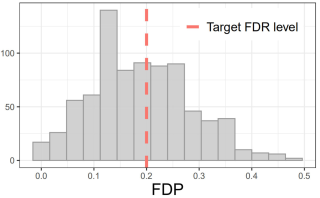
Figure 1: FDP under a given target FDR level

Despite the success of knockoff filters, some issues remain to be further investigated:

• FDR Vs. FDP and $k$-FWER. The control of FDR does not assure the control of FDP (Genovese and Wasserman 2004). To illustrate such phenomenon, we display the histogram of FDP when applying MX-Knockoff (Candès et al. 2018) in 800 randomly generated datasets in Figure 1, which shows FDP can significantly exceed the target FDR level. See Supplementary Material B for details of our simulated example and related discussions. In addition, as pointed out in (Farcomeni 2008), $k$-FWER control is more desirable than FDR control when a powerful selection result can be made.

• Coefficient-based feature statistic Vs. Coefficient-free feature statistic. Under MX-Knockoff framework, feature importance is usually measured by the coefficient difference, e.g., (Candès et al. 2018; Fan et al. 2020a, b). However, it may be difficult to obtain the feature importance from general nonlinear models (Christian 2012; Liu et al. 2020). Indeed, it is an open question to design new feature importance statistics (see Section 7.2.5 in (Candès et al. 2018)), e.g., coefficient-free statistics.

• Conditional randomization test Vs. Computational friendly test. Although the $p$-value of each feature can be calculated via the conditional randomization test, this procedure is required to train the learning model multiple times. It will cause heavy computational burdens when calculating valid $p$-values, especially in high-dimensional finite-sample case (Candès et al. 2018). Thus, it is an open question how to efficiently calculate valid $p$-values via knockoff technique (see Section 7.2.6 in (Candès et al. 2018)).

Table 1: Algorithmic properties ($\checkmark$-has the given information, $\times$-hasn’t the given information)

Properties	FX-Knockoff	MX-Knockoff	DeepPINK	RANK	PC-Knockoff	E-Knockoff (Ours)
Coefficient-free feature statistics	$\times$	$\times$	$\times$	$\times$	$\checkmark$	$\checkmark$
$k$-FWER control	$\times$	$\times$	$\times$	$\times$	$\times$	$\checkmark$
FDP control	$\times$	$\times$	$\times$	$\times$	$\times$	$\checkmark$
FDR control	$\checkmark$	$\checkmark$	$\checkmark$	$\checkmark$	$\checkmark$	$\checkmark$
Robust analysis	$\times$	$\times$	$\times$	$\checkmark$	$\times$	$\checkmark$
Power analysis (linear model)	$\times$	$\times$	$\times$	$\checkmark$	$\checkmark$	$\checkmark$
Power analysis (nonlinear model)	$\times$	$\times$	$\times$	$\times$	$\checkmark$	$\checkmark$

Main Contributions

To address the above issues, this paper proposes a new knockoff filter scheme, called Error-based Knockoffs Inference (E-Knockoff), for controlled feature selection based on the error-based feature statistics. The main contributions of this paper are summarized as below:

• Error-based knockoffs inference. Our model integrates the knockoff features (Candès et al. 2018), the error-based feature statistics and the stepdown procedure (Lehmann and Romano 2005) into a coherent way for FDR, FDP or $k$-FWER control. The error-based importance measure does not require specifying a regression model and can be used to calculate the valid $p$-values efficiently. The stepdown procedure, with the help of new importance statistics, provides the route to control FDP and $k$-FWER, respectively, which is different from the previous knockoffs inference just for FDR control (Barber and Candès 2015; Candès et al. 2018; Lu et al. 2018; Fan et al. 2020a, b; Liu et al. 2020). In particular, it is novel to design the error-based statistics of feature importance under the knockoff framework, which partially answers the open questions stated in Sections 7.2.5 and 7.2.6 (Candès et al. 2018).

• Theoretical guarantees on $k$-FWER, FDP, and FDR control. For the MX-Knockoff framework, statistical foundations on the power and FDR control have been provided in (Candès et al. 2018; Fan et al. 2020a, b), where the power analysis is limited to high-dimensional linear models with both known and unknown covariate distribution. Beyond the linear models in aforementioned literature, we state theoretical justifications on the tight $k$-FWER control and FDP control when the stepdown procedure is employed. In particular, the robustness of $k$-FWER and FDP control can also be assured even for unknown covariate distribution associated with Gaussian graphical model. Additionally, our power analysis holds for general nonlinear models, which is closely related to the open question illustrated in Section 6 (Fan et al. 2020a). Some empirical evaluations support our theoretical findings.

To better illustrate the novelty of current work, we compare it with FX-Knockoff (Barber and Candès 2015), MX-Knockoff (Candès et al. 2018), DeepPINK (Lu et al. 2018), RANK (Fan et al. 2020a), PC-Knockoff (Liu et al. 2020) in Table 1 from the lens of feature statistics, control ability, and asymptotic theory. Table 1 shows that our approach enjoys theoretical guarantees on robustness and power for FDR, FDP, and $k$-FWER control.

Preliminaries

This section introduces some necessary backgrounds including the problem setup, the knockoff filter (Candès et al. 2018) and the stepdown procedure (Lehmann and Romano 2005).

Problem Statement

Let $\mathcal{X}\subset\mathbb{R}^{p}$ be the compact input space and let $\mathcal{Y}\subset\mathbb{R}$ be the output set. We have $n$ independent identically distributed (i.i.d.) observations $\{(\mathbf{x}_{i},Y_{i})\}_{i=1}^{n}$ from the population $(\mathbf{x},Y)$, where $\mathbf{x}=(X_{1},\dots,X_{p})\in\mathcal{X}$ and $Y\in\mathcal{Y}$. Suppose that the conditional distribution of $Y$ is only relevant with a small subset of $p$ covariates.

The definition of irrelevant features is given in Candès et al. (2018).

Definition 1

(Candès et al. 2018) A feature $X_{j}$ is said to be “irrelevant” if $Y$ is independent of $X_{j}$ conditionally on

$$\mathbf{x}_{-j}:=(X_{1},\dots,X_{j-1},X_{j+1},\dots,X_{p}).$$

For simplicity, we denote it as

$$Y\rotatebox{90.0}{$\models$}X_{j}|\mathbf{x}_{-j}.$$

Remark 1

If feature $X_{j}$ is irrelevant according to Definition 1, it satisfies that the conditional distribution $Y|\mathbf{x}\overset{d}{=}Y|\mathbf{x}_{-j}$, where $\overset{d}{=}$ denotes equality in distribution. That is, the conditional distribution of  $Y$ remains invariant when removing $X_{j}$ from $\mathbf{x}$.

Let $\mathcal{S}_{1}\subset\{1,\dots,p\}$ be the index set with respect to irrelevant features. Naturally, the index set of true informative features $\mathcal{S}_{0}$ is the complement set of $\mathcal{S}_{1}$, i.e., $\mathcal{S}_{0}=\mathcal{S}_{1}^{c}$. This paper aims to find $\widehat{\mathcal{S}}$, the data dependent estimation of $\mathcal{S}_{0}$, while controlling $k$-FWER, FDP, or FDR. Recall that

$$\text{FDR}=\mathbb{E}[\text{FDP}]=\mathbb{E}\left[\frac{|\widehat{\mathcal{S}}\cap\mathcal{S}_{1}|}{|\widehat{\mathcal{S}}|\vee 1}\right]$$

and

$$\text{$k$-FWER}=Prob\{|\widehat{\mathcal{S}}\cap\mathcal{S}_{1}|\geq k\},$$

where $|\cdot|$ is the cardinality of a set.

Model-X Knockoff Framework

Model-X knockoff framework (Candès et al. 2018) aims to identify informative features while controlling FDR. The key point is to construct the knockoff copy of $\mathbf{x}$ which looks like real ones without contribution to the response.

Definition 2

(Candès et al. 2018) Model-X knockoffs for the family of random variables $\mathbf{x}=(X_{1},\dots,X_{p})$ is a new family of random variables $\tilde{\mathbf{x}}=(\tilde{X}_{1},\dots,\tilde{X}_{p})$ satisfying

$$\tilde{\mathbf{x}}\rotatebox{90.0}{$\models$}Y|\mathbf{x}$$ (1)

and

$$(\mathbf{x},\tilde{\mathbf{x}})_{swap(s)}\overset{d}{=}(\mathbf{x},\tilde{\mathbf{x}}),\forall s\subset\{1,\dots,p\}.$$ (2)

Here, $(\mathbf{x},\tilde{\mathbf{x}})=(X_{1},\dots,X_{p},\tilde{X}_{1},\dots,\tilde{X}_{p})$, and $(\mathbf{x},\tilde{\mathbf{x}})_{swap(s)}$ is swapping $X_{j}$ with $\tilde{X}_{j}$ for all $j\in s$, e.g., when $p=3$, $(\mathbf{x},\tilde{\mathbf{x}})_{swap(\{2,3\})}=(X_{1},\tilde{X}_{2},\tilde{X}_{3},\tilde{X}_{1},X_{2},X_{3})$.

Remark 2

The properties of knockoff features have been well investigated in (Candès et al. 2018). The property (1) illustrates that all knockoff features are noise features, and (2) assures the similarity between $\mathbf{x}$ and $\tilde{\mathbf{x}}$.

Candès et al. (2018) state the construction of knockoffs when $\mathbf{x}$ obeys a known Gaussian graphical model $\mathcal{N}(\mathbf{0},\mathbf{\Sigma})$, where the covariance matrix $\mathbf{\Sigma}$ is positive definite. Model-X knockoff can construct $\tilde{\mathbf{x}}$ conditionally on $\mathbf{x}$ w.r.t. $\tilde{\mathbf{x}}|\mathbf{x}\overset{d}{=}\mathcal{N}(\mu,\mathbf{V})$, where

$$\mu=\mathbf{x}(I_{p}-\mathbf{\Sigma^{-1}}\text{diag}\{\mathbf{s}\}),$$

$$\mathbf{V}=2\text{diag}\{\mathbf{s}\}-\text{diag}\{\mathbf{s}\}\mathbf{\Sigma^{-1}}\text{diag}\{\mathbf{s}\},$$

and the joined distribution of $(\mathbf{x},\tilde{\mathbf{x}})$ satisfies

$$(\mathbf{x},\tilde{\mathbf{x}})\sim\mathcal{N}(\mathbf{0},\mathbf{G})$$

with

$$\mathbf{G}=\left(\begin{array}[]{cc}\mathbf{\Sigma}&\mathbf{\Sigma}-\text{diag}\{\mathbf{s}\}\\ \mathbf{\Sigma}-\text{diag}\{\mathbf{s}\}&\mathbf{\Sigma}\end{array}\right).$$ (3)

Some strategies have been provided in (Candès et al. 2018) for selecting diagonal matrix $\text{diag}\{\mathbf{s}\}$ .

Given i.i.d. observations $\{(\mathbf{x}_{i},Y_{i})\}_{i=1}^{n}$, denote

$$\mathbf{X}=(\mathbf{x}_{i})_{i=1}^{n}\in\mathbb{R}^{n\times p}~{}~{}\mbox{and}~{}~{}\mathbf{y}=(Y_{i})_{i=1}^{n}\in\mathbb{R}^{n},$$

where each $\mathbf{x}_{i}=(X_{i1},\dots,X_{ip})$. The knockoff data matrix $\tilde{\mathbf{X}}=(\tilde{\mathbf{x}}_{i})_{i=1}^{n}$ is constructed by row w.r.t. $\tilde{\mathbf{x}}|\mathbf{x}$, where $\tilde{\mathbf{x}}_{i}$ is the knockoff copy of $\mathbf{x}_{i}$. The $n\times 2p$ matrix $[\mathbf{X},\mathbf{\tilde{X}}]$ is obtained by connecting $\mathbf{X}$ and $\tilde{\mathbf{X}}$. To identify active features, a paired-input filter is trained on $\big{(}[\mathbf{X},\tilde{\mathbf{X}}],\mathbf{y}\big{)}$, e.g, Lasso (Hastie and Tibshirani 1990) in (Candès et al. 2018). Then, each feature (including its knockoff) is assigned with a coefficient-based score, e.g., the absolute value of Lasso coefficient (Candès et al. 2018; Fan et al. 2020a).

Let $Z_{j}$ and $\tilde{Z}_{j}$ be the score of $X_{j}$ and $\tilde{X}_{j}$ respectively. The importance measure of feature $X_{j}$ is defined by

$$W_{j}:=w_{j}\big{(}[\mathbf{X},\mathbf{\tilde{X}}],\mathbf{y}\big{)}=Z_{j}-\tilde{Z}_{j},$$

where $w_{j}$ is a model-driven function associated with $[\mathbf{X},\mathbf{\tilde{X}}],\mathbf{y}$. Typical example of $W_{j}$ is the Lasso coefficient difference (LCD) used in (Candès et al. 2018; Fan et al. 2020a). The distribution of $W_{j}$ enjoys the following flip-sign property.

Proposition 1

(Candès et al. 2018) Assume swapping $X_{j}$ with $\tilde{X}_{j}$ has the effect of changing the sign of $W_{j}$, i.e.,

$$w_{j}\big{(}[\mathbf{X},\mathbf{\tilde{X}}]_{swap(\{j\})},\mathbf{y}\big{)}=-w_{j}\big{(}[\mathbf{X},\mathbf{\tilde{X}}],\mathbf{y}\big{)}.$$

Then, each $W_{j}$ associated with irrelevant feature is independent and symmetrically distributed.

The above property is helpful to obtain the theoretical guarantee on the FDR control.

Lemma 1

(Candès et al. 2018) If  $W_{j}$ is independent and symmetrically distributed for each $j\in\mathcal{S}_{1}$. For any given target FDR level $q\in(0,1)$, let

$$\tau=\min\bigg{\{}\tau>0:\frac{1+|\{j:W_{j}\leq-\tau\}|}{|\{j:W_{j}\geq\tau\}|\vee 1}\leq q\bigg{\}}.$$ (4)

Then the procedure selecting the variables $\widehat{\mathcal{S}}=\{j:W_{j}\geq\tau\}$ can control $\text{FDR}\leq q$.

Usually, the FDR control under model-X knockoff framework depends heavily on the coefficient difference derived from Lasso (Candès et al. 2018; Fan et al. 2020a), group Lasso (Sesia et al. 2020), and paired-input deep neural networks (Lu et al. 2018). In many applications involving complex function relationships, this coefficient-based property may hinder the flexibility and accuracy of model-X knockoff framework.

Stepdown Procedure

Denote $\mathcal{P}_{j}$ as the $p$-value associated with the significance of feature $X_{j},j=1,\dots,p$. Let $\mathcal{P}_{k_{j}}$, $j=1,\dots,p$, be the $p$-values with $\mathcal{P}_{k_{1}}\leq\dots\leq\mathcal{P}_{k_{p}}$ and let $\alpha_{j},j=1,\dots,p$, be the significance threshold values with $\alpha_{1}\leq\dots\leq\alpha_{p}$. Naturally, the first $m$ features with lower $p$-values are selected as informative variables $\mathcal{\widehat{S}}=\{k_{1},\dots,k_{m}\}$, where

$$m=\max\{M:\mathcal{P}_{k_{j}}\leq\alpha_{j},\forall j\leq M\}.$$

Lehmann and Romano (2005) have stated the following results about $k$-FWER and FDP control.

Lemma 2

(Lehmann and Romano 2005) For any given $\alpha\in(0,1)$ and $k=1,\dots,p$, the stepdown procedure with

$$\alpha_{j}=\left\{\begin{aligned} &\frac{k\alpha}{p},&&j\leq k\\ &\frac{k\alpha}{p+k-j},&&j>k\end{aligned}\right.$$

can control $\text{$k$-FWER}\leq\alpha$.

Lemma 3

(Lehmann and Romano 2005) For any given $\alpha,q\in(0,1)$, if the $p$-value of any irrelevant feature is independent of the $p$-values of informative features, the stepdown procedure with

$$\alpha_{j}=\frac{(\lfloor qj\rfloor+1)\alpha}{p+\lfloor qj\rfloor+1-j}$$

satisfies $Prob\{\text{FDP}>q\}\leq\alpha$.

Error-based Knockoff Inference

This paper exploits the idea of “feature replacing” for controlled feature selection, i.e., replacing a feature with its knockoff and see whether there is a significant difference in the estimation error or not. We first assume the distribution of $\mathbf{x}$ is known as prior and propose an error-based feature statistic for $k$-FWER, FDP, or FDR control. Then, we extend the theoretical result to a more general setting where the distribution of $\mathbf{x}$ is unknown. Finally, the power analysis is stated for the proposed approach.

Error-based Feature Importance

To construct the error-based feature importance $W_{j},j=1,\dots,p$, we need to divide $n$ samples into two disjointed parts: $(\mathbf{X}^{*},\mathbf{y}^{*})$ and $(\mathbf{X}^{\prime},\mathbf{y}^{\prime})$, containing $n_{1}$ and $n_{2}$ samples, respectively.

Let $f$ be the regression estimator trained on $(\mathbf{X}^{*},\mathbf{y}^{*})$ and let $\tilde{\mathbf{X}}^{\prime}$ be the knockoff copy of $\mathbf{X}^{\prime}$. Denote $\big{(}(\mathbf{x}_{i}^{\prime},\tilde{\mathbf{x}}_{i}^{\prime}),Y_{i}^{\prime}\big{)}$ as the $i$-th column of $([\mathbf{X}^{\prime},\tilde{\mathbf{X}}^{\prime}],\mathbf{y}^{\prime})$. Given an estimator $f$ and random sample $(\mathbf{x},Y)\in\mathcal{X}\times\mathcal{Y}$, define the error-based random variable

$$\xi:=\xi(\mathbf{x},Y)=|f(\mathbf{x})-Y|$$ (5)

and

$$\xi^{j}:=\xi^{j}(\mathbf{x},Y)=|f\big{(}\mathcal{R}_{j}(\mathbf{x})\big{)}-Y|,$$ (6)

where

$$\mathcal{R}_{j}(\mathbf{x})=(X_{1},\dots,X_{j-1},\tilde{X}_{j},X_{j+1},\dots,X_{p}).$$

For observation $(\mathbf{x}^{\prime}_{i},Y^{\prime}_{i})$ associated with $(\mathbf{X}^{\prime},\mathbf{y}^{\prime})$, we define

$$\xi_{i}=\left|f(\mathbf{x}^{\prime}_{i})-Y^{\prime}_{i}\right|~{}~{}\mbox{and}~{}~{}\xi_{i}^{j}=\left|f\big{(}\mathcal{R}_{j}(\mathbf{x}_{i}^{\prime})\big{)}-Y^{\prime}_{i}\right|.$$

The feature importance can be measured by the error difference between $\xi_{i}^{j}$ and $\xi_{i}$, i.e.,

$$T_{i}^{j}:=\xi_{i}^{j}-\xi_{i}.$$

The error-based feature importance can be characterized by

$$W_{j}:=\frac{1}{n_{2}}\Big{(}\sum\limits_{i=1}^{n_{2}}\rm{I}_{\{\it{T_{i}^{j}}>0\}}\Big{)}-0.5,$$ (7)

where indicator function $\rm{I}_{\{\it{A}\}}=1$ if $A$ is true and 0 otherwise.

The basic properties of $W_{j}$ are stated as below, which are obtained from the definition of knockoff features (e.g., Definition 2) and the flip-sign property of MX-Knockoff feature importance (e.g., Proposition 1). The corresponding proof can be found in Supplementary Material C.

Proposition 2

For each $j\in\mathcal{S}_{1}$, $W_{j}$ defined in (7) is independent and symmetrically distributed around zero, and satisfies $n_{2}(W_{j}+0.5)\sim\mathcal{B}(n_{2},0.5),\forall j\in\mathcal{S}_{1}$.

Remark 3

The first conclusion of Theorem 2 differs from Proposition 1 ( See also Lemma 3.3 in (Candès et al. 2018)) in that, we remove the assumption on feature importance via replacing strategy. Since the error-based importance measure has no requirement on the structure of learning machine, it may be much flexible for applications. The second conclusion reveals the distribution information of the proposed irrelevant feature’s importance, which gives us the opportunity to realize $k$-FWER control and FDP control via combining the knockoff technique with the stepdown procedure.

Combining Lemma 1 and Proposition 2 yields the following result for FDR control.

Theorem 1

For any given target FDR level $q\in(0,1)$, the error-based knockoff procedure, with feature importance (7) and knockoff threshold (4), satisfies $\text{FDR}\leq q$.

Assume the null-hypothesis that the feature is irrelevant. Let $M_{j}:=\max\{n_{2}(W_{j}+0.5),n_{2}(0.5-W_{j})\}$. The $p$-values are defined as

$$\mathcal{P}_{j}:=2\sum\limits_{i=M_{j}}^{n_{2}}C(n_{2},i)\frac{1}{2^{n_{2}}},j=1,\dots,p$$ (8)

are used to evaluate the feature significance, where $C(n_{2},m)$ is the combinatorial number.

The following theoretical results on $k$-FWER and FDP control can be established by combining Proposition 2 with Lemmas 2 and 3.

Theorem 2

For any given $\alpha\in(0,1)$, the stepdown procedure, constructed in Lemma 2 and associated with knockoff-based $p$-values (8), satisfies $\text{$k$-\text{FWER}}\leq\alpha$.

Theorem 3

For any given $q,\alpha\in(0,1)$, the FDP of $\widehat{\mathcal{S}}$, associated with the stepdown procedure in Lemma 3 and $p$-values in (8), satisfies $Prob\{\text{FDP}>q\}\leq\alpha$.

Remark 4

Different from the previous knockoff filters relied on the coefficient difference (Barber and Candès 2015; Candès et al. 2018; Lu et al. 2018; Barber and Candès 2019), the current knockoff procedure rooted in the error difference. The error-based knockoff strategy is model-free (no structure restriction on estimator $f$), and gives us the opportunity to tackle FDR, FDP, and $k$-FWER control.

Algorithm 1 Construct feature importance statistic $W_{j}$

Input: Data $(\mathbf{X}^{\prime},\mathbf{y}^{\prime})$, trained filter $f$, feature index $j$
Output: Feature importance statistic $W_{j}$

1:  Construct $\mathbf{\tilde{X}}^{\prime}$, i.e., the knockoff copy of $\mathbf{X}^{\prime}$.

2:  for $i=1,\dots,n_{2}$ do

3:     Obtain $\mathcal{R}_{j}(\mathbf{x}^{\prime}_{i})$ by replacing $j$-th feature in $\mathbf{x}^{\prime}_{i}$ with its knockoff copy.

4:     $T_{i}^{j}\leftarrow\left|f\big{(}\mathcal{R}_{j}(\mathbf{x}^{\prime}_{i})\big{)}-Y^{\prime}_{i}\right|-|f(\mathbf{x}^{\prime}_{i})-Y^{\prime}_{i}|$

5:  end for

6:  $W_{j}\leftarrow\frac{1}{n_{2}}\left(\sum\limits_{i=1}^{n_{2}}\rm{I}_{\{\it{T_{i}^{j}}>0\}}\right)-0.5.$

7:  return  $W_{j}$

Robustness Analysis

This section further establishes the asymptotic properties of $k$-FWER control and FDP control when the distribution of $\mathbf{x}$ is characterized by some unknown Gaussian graphical model, i.e., $\mathbf{x}\sim\mathcal{N}(\mathbf{0},\mathbf{\Sigma})$. All proofs of this section have been provided in Supplementary Material C.

Let $\mathbf{\widehat{\Sigma}}$ be the empirical estimation of covariance matrix obtained by $(\mathbf{X}^{*},\mathbf{y}^{*})$. To ease the presentation, for any notation $\mathbf{A}$ associated with the unknown covariance matrix $\mathbf{\Sigma}$, the notation $\widehat{\mathbf{A}}$ stand for its empirical estimation constructed via $\widehat{\mathbf{\Sigma}}$. Inspired from Fan et al. (2020a), we introduce the following conditions for our robustness analysis.

The following condition on density function is required, which holds true for bounded regression problem with Gaussian noise assumption (Tibshirani 1996; Yuan and Lin 2006; Meier, Van De Geer, and Bü hlmann 2008; Christian 2012).

Condition 1

Let $\eta(Y|\mathbf{x})$ be the probability density function of $Y$ conditioned on $\mathbf{x}$. There holds $\max\limits_{(\mathbf{x},Y)}\eta(Y|\mathbf{x})\leq C_{1}$ for some constant $C_{1}$.

Without loss of generality, assume the covariance matrix $\mathbf{G}$ defined in (3) to be positive definite (Fan et al. 2020a). The following condition is used to characterize the relationship between $\mathbf{G}$ and its empirical estimation $\widehat{\mathbf{G}}$, and to rule out some extreme case of these matrixs, e.g., $\lambda_{max}(\mathbf{G})=\infty$. Similar condition has been used in (Fan et al. 2020a) for robust analysis.

Condition 2

Let $\lambda_{min}(\cdot)$ and $\lambda_{max}(\cdot)$ be the minimum and the maximum matrix eigenvalues, respectively. There exist some positive sequence $a_{n_{1}},b_{n_{1}}$ satisfying $a_{n_{1}}\rightarrow 0,b_{n_{1}}\rightarrow 0$ as $n_{1}\rightarrow\infty$, and a positive constant $C_{2}$ such that

$$\|\widehat{\mathbf{G}}-\mathbf{G}\|_{2}\leq a_{n_{1}}$$

and

$$\begin{split}\frac{1}{C_{2}}\leq&\min\bigg{\{}\lambda_{\min}(\mathbf{G}),\lambda_{\min}(\mathbf{\widehat{G}})\bigg{\}}\\ \leq&\max\bigg{\{}\lambda_{\max}(\mathbf{G}),\lambda_{\max}(\mathbf{\widehat{G}})\bigg{\}}\leq C_{2}\end{split}$$

with probability at least $1-p^{-\frac{1}{b_{n_{1}}}}$.

Table 2: Results on the simulated data for controlled feature selection (different dimension $p$)

$p$	E-Knockoff($k$-FWER)			E-Knockoff(FDP)			E-Knockoff(FDR)			MX-Knockoff			DeepPINK
	$\text{FDP}_{\max}$	FDR	Power	$\text{FDP}_{\max}$	FDR	Power	$\text{FDP}_{\max}$	FDR	Power	$\text{FDP}_{\max}$	FDR	Power	$\text{FDP}_{\max}$	FDR	Power
50	0.03	0.01	1.00	0.12	0.03	1.00	0.35	0.19	1.00	0.33	0.20	1.00	0.32	0.20	1.00
100	0.03	0.00	0.97	0.17	0.04	1.00	0.40	0.19	1.00	0.45	0.19	1.00	0.52	0.17	1.00
200	0.07	0.00	0.95	0.14	0.04	0.99	0.48	0.20	1.00	0.45	0.20	1.00	0.36	0.16	1.00
400	0.04	0.01	0.91	0.13	0.04	0.98	0.43	0.19	1.00	0.39	0.19	1.00	0.50	0.22	1.00
800	0.07	0.01	0.63	0.13	0.04	0.83	0.36	0.19	0.95	0.40	0.20	1.00	0.33	0.18	1.00
1200	0.06	0.00	0.60	0.08	0.03	0.79	0.42	0.16	0.93	0.40	0.16	1.00	0.38	0.19	1.00
1600	0.07	0.01	0.59	0.17	0.04	0.79	0.40	0.18	0.94	0.35	0.19	1.00	0.44	0.18	1.00
2000	0.07	0.01	0.57	0.13	0.03	0.77	0.52	0.19	0.92	0.41	0.16	1.00	0.44	0.24	0.94

Let $\tilde{\mathbf{x}}^{\widehat{\mathbf{\Sigma}}}$ be the knockoff feature based on the distribution $\mathcal{N}(\mathbf{0},\widehat{\mathbf{\Sigma}})$. For feasibility, denote $\eta_{\mathbf{\Sigma}}$ and $\eta_{\mathbf{\widehat{\Sigma}}}$ be the distribution density function of $(\mathbf{x},\tilde{\mathbf{x}})$ and $(\mathbf{x},\tilde{\mathbf{x}}^{\widehat{\mathbf{\Sigma}}})$ respectivly. The relationship between $\eta_{\mathbf{\Sigma}}$ and $\eta_{\mathbf{\widehat{\Sigma}}}$ is described as below.

Lemma 4

Under Condition 2, there holds

$$|\eta_{\mathbf{\Sigma}}(\mathbf{x},\mathbf{\tilde{x}})-\eta_{\mathbf{\widehat{\Sigma}}}(\mathbf{x},\mathbf{\tilde{x}})|\leq O(a_{n_{1}}),\forall(\mathbf{x},\mathbf{\tilde{x}})\in\mathcal{X}^{2}$$

with probability at least $1-p^{-\frac{1}{b_{n_{1}}}}$.

It is a position to present the main results on robustness analysis for controlled variable selection.

Theorem 4

Let Conditions 1 and 2 be true. For any given $\alpha\in(0,1),k=1,\dots,p$ and $n_{2}\in\mathbb{R}$, the feature seleciton procedure described in Theorem 2 satisfies

$$\widehat{\text{$k$-FWER}}\leq\alpha+O(p^{-\frac{1}{b_{n_{1}}}})+O(a_{n_{1}}).$$

Theorem 5

Let Conditions 1 and 2 be true. For any given $q,\alpha\in(0,1)$, $n_{2}\in\mathbb{R}$, the feature selection procedure described in Theorem 3 satisfies

$$Prob\{\widehat{\text{FDP}}>q\}\leq\alpha+O(p^{-\frac{1}{b_{n_{1}}}})+O(a_{n_{1}}).$$

Table 3: Maximum number of false discoveries in 50 trials

method	50	100	200	400	800	1200	1600	2000
E-Knockoff($k$-FWER)	1	1	2	1	1	1	1	1

Remark 5

Theorems 4 and 5 guarantee the robustness of our error-based knockoff inference under mild conditions. Here, we omit the robust analysis for FDR control since it can be derived directly from (Fan et al. 2020a). To the best of our knowledge, there is no robust analysis for FDP and $k$-FWER control under the knockoff filtering framework.

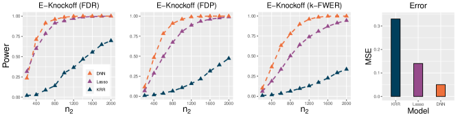
Figure 2: Power analysis (Power Vs. $n_{2}$) on the simulated data for different learning models

Power Analysis

The following restriction on the predictor $f$ is involved for the power property of our error-based knockoff inference.

Condition 3

For the error-based random variables $\xi$ in (5) and $\xi^{j}$ in (6), there holds

$$Prob\{\xi^{j}>\xi\}>Prob\{\xi^{j}<\xi\},\forall j\in\mathcal{S}_{0}.$$

Condition 3 ensures that the predictor $f$ would have degraded performance when replacing an informative feature with a knockoff feature. Recall that the construction procedure of knockoffs is independent of the response $Y$, see e.g., Candès et al. (2018); Romano, Sesia, and Candès (2019); Jordon, Yoon, and Mihaela (2019). Therefore, the current restriction on $f$ is mild since less information is more likely to result in additional prediction loss.

The central limit theorem assures that the variance of proposed feature importance in (7) would converge to zero. Thus, we get the following result.

Theorem 6

Under Condition 3, the feature selection procedures described in Theorem 1-3 satisfy

$$\text{Power}:=\mathbb{E}\left[\frac{|\widehat{\mathcal{S}}\cap\mathcal{S}_{0}|}{|\mathcal{S}_{0}|}\right]\rightarrow 1~{}~{}\mbox{as}~{}~{}n_{2}\rightarrow\infty.$$

Remark 6

Theorem 6 demonstrates that the power of proposed procedures depends on the sample size $n_{2}$ of $(\mathbf{X}^{\prime},\mathbf{y}^{\prime})$. Theorems 4-6 imply that, for our error-based knockoff inference, there is a tradeoff between $n_{1}$ (associated with getting the predictor $f$ and covarince matrix $\mathbf{\widehat{\Sigma}}$) and $n_{2}$ (related to generate knockoffs and error-based feature statistic $W_{j}$).

Experimental Analysis

This section states empirical evaluations of our error-based knockoff inference on both synthetic data and HIV dataset (Rhee et al. 2006) to valid our theoretical claims about controlled feature selection and power analysis. The detailed experiment settings and some additional experiments are provided in Supplementary Material D.

Simulated Data Evaluation

Inspired by (Lu et al. 2018), we draw $\mathbf{x}$ independently from $\mathcal{N}(\mathbf{0},\mathbf{\Sigma})$, where $\mathbf{\Sigma}^{-1}=(0.5^{|j-k|})_{1\leq j,k\leq p}$. Then, we simulate the response from single index model:

$$Y=g(\mathbf{x}\beta)+\epsilon,~{}~{}\epsilon\sim\mathcal{N}(0,0.01)$$

where the linkage function

$$g(a)=\sqrt{|a|}+a+a^{2}+\text{sin}(a)+\text{arctan}(a),\forall a\in\mathbb{R},$$

$\beta=(\beta_{1},\dots,\beta_{p})^{T}$ satisfying $\beta_{j}=0,\forall j\in\mathcal{S}_{1}$ and $\beta_{j}=1/|\mathcal{S}_{0}|$ otherwise. Here, the sample size $n=2000$ and the number of features $p\in\{50,100,200,400,800,1200,1600,2000\}$ with $|\mathcal{S}_{0}|=30$ (Lu et al. 2018).

This paper employes the coefficient-based model-X knockoff (Candès et al. 2018) and DeepPink (Lu et al. 2018) as the baselines. We set the target FDR level $q=0.2$ for all FDR controlled methods, set $q=0.2$ and $\alpha=0.2$ for FDP control version of E-Knockoff (E-Knockoff (FDP)), and set $k=2$ and $\alpha=0.1$ for $k$-FWER control version of E-Knockoff (E-Knockoff ($k$-FWER)). The feature importance is measured by the coefficient difference associated with Lasso for MX-Knockoff (Candès et al. 2018) and associated with paired-input DNNs for DeepPink (Lu et al. 2018). We use Lasso as the base estimator of our E-Knockoff inference with $n_{1}=n_{2}=1000$. Table 2 summaries the estimation of FDR, Power and the maximum value of FDP ($\text{FDP}_{\max}$) with 50 repetitions. In addition, Table 6 reports the max number of false discoveries for E-Knockoff ($k$-FWER) in these trials. These experimental results show that our error-based knockoff inference can reach the FDR control, FDP control, and $k$-FWER control flexibily, while MX-Knockoff and DeepPINK just can control the FDR. Meanwhile, E-Knockoff (FDP) and E-Knockoff ($k$-FWER) also enjoy the promising selection accuracy in almost all settings.The results of Table 2 also verify the tradeoff between accuracy and power discussed in (Korn et al. 2004; Lehmann and Romano 2005; Farcomeni 2008).

To verify the model-free property and power ability of our approach, we provide an experiment to illusrate the influence of $n_{2}$ and $f$ on selection results. We set $p=800,n_{1}=1000$ and select $n_{2}$ from $\{200,400,600,800,\dots,2000\}$. Three classic learning machines are used to get $f$ including Deep neural networks (DNN) (Hinton and Salakhutdinov 2006), Lasso (Tibshirani 1996) and Kernel ridge regression (KRR) (Christian 2012). Experimental results of power and mean square error (MSE) are displaced in Figure 2 after repeating the each experiment 30 times. Full simulated results are presented in Supplementary Material D. It can be observed that a powerful selection result can be made with the increase of $n_{2}$, which supports our conclusion in Theorem 6. Also, the result implies that a better-trained filter can select true active features with less samples.

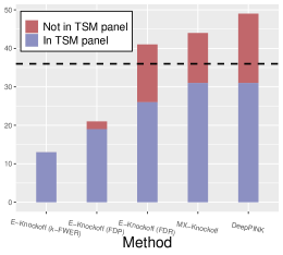
Figure 3: Results on the HIV-1 drug resistance dataset. For FPV drug class, we show the number of mutation positions for PI identified by different knockoff filters. The color indicates whether or not the selected position appears in the TSM panel, and the horizontal line shows the total number of positions on the TSM panel.

Real Data Evaluation

We next apply E-Knockoff to identify key mutations of HIV associated with the drug resistance (Rhee et al. 2006). The HIV-1 dataset consists of the data of the drug resistance level, mutations, and the treatment-selected mutations (TSM) associated with drug resistance. For each drug, the response $Y$ is the log-transformed drug resistance level, and the $j$-th feature of argument $\mathbf{x}$ indicates the presence or absence of the $j$-th mutation (Lu et al. 2018; Li et al. 2021). Figure 4 summarizes the experimental results related to FPV drugs resistance (with 1809 samples and 224 dimensions), and Supplementary Material D reports the results of other drugs. Here, we use Lasso as the base estimator for E-Knockoff inference ($n_{1}=\frac{n}{3},n_{2}=\frac{2n}{3}$). We set $k=2,\alpha=0.1$ for E-Knockoff ($k$-FWER), $q=0.2,\alpha=0.2$ for E-Knockoff (FDP), and $q=0.2$ for E-Knockoff (FDR), MX-Knockoff, and DeepPINK. Empirical results demonstrate that the error-based knockoff inference can usually control the false discovery efficiently.

Conclusion

To improve the adaptivity and flexibility of the model-X knockoff framework, this paper proposes a new error-based knockoff inference method for controlled feature selection. We establish the statistical asymptotic analysis and power analysis of the proposed approach. Empirical evaluations demonstrate the competitive performance of the proposed procedure on simulated and real data, which support our research motivation and theoretical findings. In the future, it is interesting to extend the current work for multi-environment controlled feature selection (Li et al. 2021).

Supplementary Material A

To improve the readability, we summarize the main notations of this paper in Table 4.

Table 4: Notations

Notations	Descriptions
$\mathcal{X},\mathcal{Y}$	the compact input space and output space, respectively
$\mathbf{x},Y$	the random variables taking values from $\mathcal{X}$ and $\mathcal{Y}$, respectively
$n$	sample size
$p$	the number of features in $\mathbf{x}$
$\mathbf{X},\mathbf{y}$	the data matrix and data vector assembled by $n$ i.i.d. pairs of $(\mathbf{x},Y)$
$\mathbf{X}^{*},\mathbf{y}^{*}$	the data matrix for training the predictor $f$ and covarince matrix $\widehat{\mathbf{\Sigma}}$
$\mathbf{X}^{\prime},\mathbf{y}^{\prime}$	the data matrix and data vector related to generating knockoffs and error-based feature statistic
$\tilde{\mathbf{x}},\tilde{\mathbf{X}}^{\prime}$	the knockoff copies of $\mathbf{x}$ and $\mathbf{X}^{\prime}$, respectively
$\mathcal{S}_{0},\mathcal{S}_{1}$	the set of index for informative features and irrelevant features, respectively
$\widehat{\mathcal{S}}$	the data dependent estimation of $\mathcal{S}_{0}$
$W_{j},\mathcal{P}_{j}$	the knockoff based feature importance and $p$-value for feature $X_{j}$, respectively
$\mathbf{\Sigma}$	the true covariance matrix of $\mathbf{x}$
$\mu,\mathbf{V}$	the mean and covariance matrix of the conditional distribution $\tilde{\mathbf{x}}|\mathbf{x}$, respectively
$\mathbf{G}$	the covariance matrix of joined random variables $(\mathbf{x},\tilde{\mathbf{x}})$

Supplementary Material B

B.1 Detail experiment settings of Figure 1

We randomly generated 800 datasets $\{(\mathbf{x}_{i}^{m},Y_{i}^{m})\}_{i=1}^{2000},m=1,\dots,800$, where each dataset contains 2000 i.i.d. observations with 370 irrelevant features and 30 informative features. For each observation $(\mathbf{x}_{i}^{m},Y_{i}^{m})$, the covariate $\mathbf{x}_{i}^{m}$ is drawn from $\mathcal{N}(\mathbf{0},\mathbf{\Sigma})$ with $\mathbf{\Sigma}^{-1}=(0.5^{|j-k|})_{1\leq j,k\leq 400}$ and the response $y_{i}^{m}$ is generated from single index model:

$$Y_{i}^{m}=g(\mathbf{x}_{i}^{m}\beta)+\epsilon.$$

Here the linkage function

$$g(a)=\sqrt{|a|}+a+a^{2}+\text{sin}(a)+\text{arctan}(a),~{}~{}\epsilon\sim\mathcal{N}(0,0.01)$$

with $a\in\mathbb{R},\beta=(\beta_{1},\dots,\beta_{400})^{T}$ satisfying $\beta_{j}=1/|\mathcal{S}_{0}|,\forall j\in\{1,\dots,30\}$ and $\beta_{j}=0$ otherwise.

Figure 1 displays the histogram of FDP over 800 datasets based on the MX-Knockoff filter (Candès et al. 2018), which demonstrates the control of FDR does not assure the control of FDP.

B.2 Relationship between FDR and FDP

The connection between FDR control and FDP control has been well discussed in (Korn et al. 2004; Lehmann and Romano 2005; Romano and Shaikh 2006; Luo et al. 2020).

Romano and Shaikh (2006) proved that if a method controls the FDR at a target level $q$, then

$$Prob\Big{\{}\text{FDP}>\frac{q}{\alpha}\Big{\}}\leq\alpha.$$

Obviously, this is result is not tight enough, because the radio $q/\alpha$ can be quite large for very small $\alpha$ (Romano and Shaikh 2006; Korn et al. 2004; Lehmann and Romano 2005). Moreover, if one insists on controlling FDP via some FDR control methods, the target FDR level may be too restrictive to produce a powerful selection result, e.g., under the experiment settings of B.1 with target level $0.02$, only two informative features are selected by MX-Knockoff ($\alpha=0.1$, $q/\alpha=0.2$ and $q=0.02$).

On the other hand, if a method ensures $Prob\{\text{FDP}>q\}\leq\alpha$, Lehmann and Romano (2005) established that

$$\text{FDR}=\mathbb{E}(\text{FDP})\leq q+(1-q)\alpha.$$

Supplementary Material C

Before providing the proofs of Theorems 4-6, we first establish stepping stones including Propositions 2-3 and Lemmas 4-5.

The following lemma (See also the proof of Lemma 1 in (Candès et al. 2018)) is key to prove Proposition 2.

Lemma 5

(Candès et al. 2018) For any subset $s\subset\mathcal{S}_{1}$, there holds

$$\big{(}(\mathbf{x},\mathbf{\tilde{x}}),Y\big{)}\overset{d}{=}\big{(}(\mathbf{x},\mathbf{\tilde{x}})_{swap(s)},Y\big{)}.$$

Proof of Proposition 2: The proof proceeds similarly to Lemma 2 in Section 3.2 (Candès et al. 2018).

Recall that the error difference $T_{i}$ depends on the response, the original input and its knockoffs, i.e.,

$$T_{i}=(T_{i}^{1},\dots,T_{i}^{p}):=t\big{(}(\mathbf{x}^{\prime}_{i},\tilde{\mathbf{x}}^{\prime}_{i}),Y^{\prime}_{i}\big{)}$$

for some model-based function $t(\cdot,\cdot)$. Let $\epsilon=(\epsilon_{1},\dots,\epsilon_{p})$ be a sequence of independent variables such that $\epsilon_{j}=\pm 1$ with probability $\frac{1}{2}$ if $j\in\mathcal{S}_{1}$, and $\epsilon_{j}=1$ otherwise. To prove the claim, it will suffice to establish that

$$T_{i}\overset{d}{=}\epsilon\odot T_{i},$$

where $\odot$ denotes the point-wise multiplication of vectors $\epsilon$ and $T_{i}$.

Let $s=\{j:\epsilon_{j}=-1\}$ and consider the swapping feature associated with $s$:

$$T_{i}^{swap(s)}:=t\big{(}(\mathbf{x}_{i}^{\prime},\tilde{\mathbf{x}}_{i}^{\prime})_{swap(s)},Y_{i}^{\prime}\big{)}.$$

The construction of $T_{i}$ assures that $\epsilon\odot T_{i}=T_{i}^{swap(s)}$ and Lemma 5 implies $T_{i}\overset{d}{=}T_{i}^{swap(s)}$. The desired result follows by combining the above equations.   $\Box$

The following proposition is used in our proof of Lemma 4.

Proposition 3

Suppose that $||\widehat{\mathbf{G}}-\mathbf{G}||_{2}\leq a_{n_{1}}$ and

$$\frac{1}{C_{2}} \leq \min\big{\{}\lambda_{\min}(\mathbf{G}),\lambda_{\min}(\mathbf{\widehat{G}})\big{\}}$$

$$\leq \max\big{\{}\lambda_{\max}(\mathbf{G}),\lambda_{\max}(\mathbf{\widehat{G}})\big{\}}\leq C_{2}.$$

Then, we have

$$\big{|}e^{-\frac{1}{2}(\mathbf{x},\tilde{\mathbf{x}})\mathbf{G}^{-1}(\mathbf{x},\tilde{\mathbf{x}})^{T}}-e^{-\frac{1}{2}(\mathbf{x},\tilde{\mathbf{x}})\mathbf{\widehat{G}}^{-1}(\mathbf{x},\tilde{\mathbf{x}})^{T}}\big{|}\leq O(a_{n_{1}})$$

and

$$|det(\mathbf{G})-det(\widehat{\mathbf{G}})|\leq O(a_{n_{1}}).$$

Proof of Proposition 3: The proof steps used here are inspired by the proof of Proposition 1 in (Fan et al. 2020a). Based on the matrix norm inequality, we have

$$\big{|}(\mathbf{x},\tilde{\mathbf{x}})\mathbf{G}^{-1}(\mathbf{x},\tilde{\mathbf{x}})^{T}-(\mathbf{x},\tilde{\mathbf{x}})\mathbf{\widehat{G}}^{-1}(\mathbf{x},\tilde{\mathbf{x}})^{T}\big{|}$$

$$= \big{|}\big{|}(\mathbf{x},\tilde{\mathbf{x}})\mathbf{G}^{-1}(\mathbf{x},\tilde{\mathbf{x}})^{T}-(\mathbf{x},\tilde{\mathbf{x}})\mathbf{\widehat{G}}^{-1}(\mathbf{x},\tilde{\mathbf{x}})^{T}\big{|}\big{|}_{2}$$

$$\leq \big{|}\big{|}(\mathbf{x},\tilde{\mathbf{x}})\big{|}\big{|}_{2}\cdot\big{|}\big{|}\mathbf{G}^{-1}(\mathbf{x},\tilde{\mathbf{x}})^{T}-\mathbf{\widehat{G}}^{-1}(\mathbf{x},\tilde{\mathbf{x}})^{T}\big{|}\big{|}_{2}$$

$$\leq \big{|}\big{|}(\mathbf{x},\tilde{\mathbf{x}})\big{|}\big{|}_{2}\cdot\big{|}\big{|}\mathbf{G}^{-1}-\mathbf{\widehat{G}}^{-1}\big{|}\big{|}_{2}\cdot\big{|}\big{|}(\mathbf{x},\tilde{\mathbf{x}})^{T}\big{|}\big{|}_{2}$$

$$\leq \big{|}\big{|}(\mathbf{x},\tilde{\mathbf{x}})\big{|}\big{|}_{2}\cdot\big{|}\big{|}(\mathbf{x},\tilde{\mathbf{x}})^{T}\big{|}\big{|}_{2}$$

$$\cdot\big{|}\big{|}\mathbf{G}^{-1}\big{|}\big{|}_{2}\cdot\big{|}\big{|}\mathbf{\widehat{G}}-\mathbf{G}\big{|}\big{|}_{2}\cdot\big{|}\big{|}\mathbf{\widehat{G}}^{-1}\big{|}\big{|}_{2}$$

$$\leq O(a_{n_{1}}).$$

Then,

$$\big{|}e^{-\frac{1}{2}(\mathbf{x},\tilde{\mathbf{x}})\mathbf{G}^{-1}(\mathbf{x},\tilde{\mathbf{x}})^{T}}-e^{-\frac{1}{2}(\mathbf{x},\tilde{\mathbf{x}})\mathbf{\widehat{G}}^{-1}(\mathbf{x},\tilde{\mathbf{x}})^{T}}\big{|}$$

$$\leq e^{-\frac{1}{2}(\mathbf{x},\tilde{\mathbf{x}})\mathbf{G}^{-1}(\mathbf{x},\tilde{\mathbf{x}})^{T}}\cdot\big{|}1-e^{O(a_{n_{1}})}\big{|}$$

$$\leq O(a_{n_{1}}).$$

This proves the first statement of Proposition 3.

Let $\mathbf{G}=(g_{ij})_{1\leq i,j\leq p}$ and $\mathbf{\widehat{G}}=(\hat{g}_{ij})_{1\leq i,j\leq p}$. Clearly $|g_{ij}-\hat{g}_{ij}|\leq O(a_{n_{1}})$. Denote $\mathbf{G}_{k}=(g_{ij}^{k})_{1\leq i,j\leq k}$ be the $k$-order submatrix of $\mathbf{G}$. Suppose inductively that $|det(\mathbf{G}_{k})-det(\mathbf{\widehat{G}}_{k})|\leq O(a_{n_{1}})$ and let $\mathbf{G}^{i1}_{k}$ be the cofactor of $\mathbf{G}_{k+1}$ with respect to $g_{i1}^{k+1}$. Moreover, we have

$$\big{|}det(\mathbf{G}_{k+1})-det(\mathbf{\widehat{G}}_{k+1})\big{|}$$

$$= \big{|}\sum\limits_{i=1}^{k+1}\left(g^{i1}_{k}\mathbf{G}^{i1}_{k}-\hat{g}_{i1}^{k+1}\widehat{\mathbf{G}}^{i1}_{k}\right)\big{|}$$

$$\leq \big{|}\sum\limits_{i=1}^{k+1}\left((g_{i1}^{k+1}-\hat{g}_{i1}^{k+1}){\mathbf{G}}^{i1}_{k}\right)\big{|}+\big{|}\sum\limits_{i=1}^{k+1}\left(\hat{g}_{i1}^{k+1}({\mathbf{G}}^{i1}_{k}-\widehat{\mathbf{G}}^{i1}_{k})\right)\big{|}$$

$$\leq O(a_{n_{1}}).$$

Thus, the second desired result follows by the principle of induction.

$\Box$

Proof of Lemma 4: From Proposition 3, we can deduce that

$$\big{|}\eta_{\mathbf{\Sigma}}(\mathbf{x},\tilde{\mathbf{x}})-\eta_{\mathbf{\widehat{\Sigma}}}(\mathbf{x},\tilde{\mathbf{x}})\big{|}$$

$$= \left|\frac{e^{-\frac{1}{2}(\mathbf{x},\tilde{\mathbf{x}})\mathbf{G}^{-1}(\mathbf{x},\tilde{\mathbf{x}})^{T}}}{\sqrt{(2\pi)^{2p}\cdot det(\mathbf{G})}}-\frac{e^{-\frac{1}{2}(\mathbf{x},\tilde{\mathbf{x}})\mathbf{\widehat{G}}^{-1}(\mathbf{x},\tilde{\mathbf{x}})^{T}}}{\sqrt{(2\pi)^{2p}\cdot det(\mathbf{\widehat{G}})}}\right|$$

$$\leq \frac{\left|\sqrt{det(\mathbf{\widehat{G}})}\big{(}e^{-\frac{1}{2}(\mathbf{x},\tilde{\mathbf{x}})\mathbf{\widehat{G}}^{-1}(\mathbf{x},\tilde{\mathbf{x}})^{T}}-e^{-\frac{1}{2}(\mathbf{x},\tilde{\mathbf{x}})\mathbf{G}^{-1}(\mathbf{x},\tilde{\mathbf{x}})^{T}}\big{)}\right|}{\sqrt{(2\pi)^{2p}det(\mathbf{\widehat{G}})\cdot det(\mathbf{G})}}$$

$$+\frac{\left|(\sqrt{det(\mathbf{\widehat{G}})}-\sqrt{det(\mathbf{G})})\cdot e^{-\frac{1}{2}(\mathbf{x},\tilde{\mathbf{x}})\mathbf{G}^{-1}(\mathbf{x},\tilde{\mathbf{x}})^{T}}\right|}{\sqrt{(2\pi)^{2p}det(\mathbf{\widehat{G}})\cdot det(\mathbf{G})}}$$

$$\leq O(a_{n_{1}}),$$

where the last two inequalities hold with probability at least $1-p^{-\frac{1}{b_{n_{1}}}}$.

$\Box$

Proof of Theorem 4: To derive this claim, it’s sufficient to establish that, for any given filter $f$,

$$\widehat{\text{$k$-FWER}}\leq\alpha+O(p^{-\frac{1}{b_{n_{1}}}})+O(a_{n_{1}}).$$

For any fixed filter $f$, denote $\Gamma$ a set of data matrix satisfying $|\widehat{\mathcal{S}}\cap\mathcal{S}_{0}|\geq k$ iff $([\mathbf{X}^{\prime},\mathbf{\tilde{X}}^{\prime}],\mathbf{y}^{\prime})\in\Gamma$. In terms of the conditional independence of knockoff feature, we have

$$k\text{-FWER} =Prob\{\big{(}[\mathbf{X}^{\prime},\mathbf{\tilde{X}}^{\prime}],\mathbf{y}^{\prime}\big{)}\in\Gamma\}$$

$$=\int\limits_{\Gamma}\prod_{i=1}^{n_{2}}\bigg{(}\eta(Y_{i}^{\prime}|\mathbf{x}_{i}^{\prime})\eta_{\mathbf{\Sigma}}(\mathbf{x}_{i}^{\prime},\tilde{\mathbf{x}}_{i}^{\prime})\bigg{)}$$

$$\leq\alpha.$$

Let $(\mathbf{\tilde{X}}^{\prime})^{\widehat{\mathbf{\Sigma}}}$ be the Knockoff data matrix constructed via $\widehat{\mathbf{\Sigma}}$. Then, $\widehat{\text{$k$-FWER}}$ can be rewritten as

$$\widehat{\text{$k$-FWER}} =Prob\{\big{(}[\mathbf{X}^{\prime},(\mathbf{\tilde{X}}^{\prime})^{\widehat{\mathbf{\Sigma}}}],\mathbf{y}^{\prime}\big{)}\in\Gamma\}$$

$$=\int\limits_{\Gamma}\prod_{i=1}^{n_{2}}\bigg{(}\eta(Y_{i}^{\prime}|\mathbf{x}_{i}^{\prime})\eta_{\widehat{\mathbf{\Sigma}}}(\mathbf{x}_{i}^{\prime},\tilde{\mathbf{x}}_{i}^{\prime})\bigg{)}.$$

Set $\mathcal{A}=\{\eta_{\mathbf{\widehat{\Sigma}}}:\big{|}\eta_{\mathbf{\Sigma}}(\mathbf{x},\tilde{\mathbf{x}})-\eta_{\mathbf{\widehat{\Sigma}}}(\mathbf{x},\tilde{\mathbf{x}})\big{|}\leq O(a_{n_{1}})\}$. We can deduce that

$$\widehat{k\text{-FWER}}\bigg{|}\eta_{\mathbf{\widehat{\Sigma}}}\in\mathcal{A}\leq \int\limits_{\Gamma}\prod_{i=1}^{n_{2}}\bigg{(}\eta(Y_{i}^{\prime}|\mathbf{x}_{i}^{\prime})\cdot\big{(}\eta_{\mathbf{\Sigma}}(\mathbf{x}_{i}^{\prime},\tilde{\mathbf{x}}_{i}^{\prime})+O(a_{n_{1}})\big{)}\bigg{)}$$

$$\leq \alpha+O(a_{n_{1}}).$$

Moreover,

$$\widehat{\text{$k$-FWER}}\leq \big{(}\widehat{k\text{-FWER}}\big{|}\eta_{\mathbf{\widehat{\Sigma}}}\in\mathcal{A}\big{)}\cdot Prob\{\eta_{\mathbf{\widehat{\Sigma}}}\in\mathcal{A}\}$$

$$+1\cdot Prob\{\eta_{\mathbf{\widehat{\Sigma}}}\not\in\mathcal{A}\}$$

$$\leq \alpha+O(a_{n_{1}})+O(p^{-\frac{1}{b_{n_{1}}}}).$$

This completes the proof.

$\Box$

We omit the proof of Theorem 5 here since its steps are similar with Theorem 4.

Proof of Theorem 6: denote the set of informative features as

$$\mathcal{S}_{0}=\{d_{1},\dots,d_{|\mathcal{S}_{0}|}\}$$

and denote

$$\epsilon_{d_{j}}=Prob\{\xi_{d_{j}}>\xi\}-0.5.$$

For $n_{2}\rightarrow\infty$, the central limit theorem implies

$$W_{d_{j}}\overset{d}{\longrightarrow}\mathcal{N}(\epsilon_{d_{j}},\sigma_{d_{j}}^{2}),$$ (9)

where $\sigma_{d_{j}}^{2}\leq\frac{0.25}{n_{2}}$.

Hence, we have

$$Prob\{W_{d_{j}}>\frac{\epsilon_{d_{j}}}{2}\}> Prob\{\frac{\epsilon_{d_{j}}}{2}<W_{d_{j}}<\frac{3\epsilon_{d_{j}}}{2}\}$$

$$= Prob\{|W_{d_{j}}-\epsilon_{d_{j}}|<\frac{\epsilon_{d_{j}}}{2}\}$$

$$\geq 1-\frac{4\sigma_{d_{j}}^{2}}{\epsilon_{d_{j}}^{2}}$$

$$\geq 1-\frac{1}{n_{2}\cdot\epsilon_{d_{j}}^{2}}$$

and $Prob\{W_{d_{j}}>\frac{\epsilon_{d_{j}}}{2}\}\rightarrow 1$ as as $n_{2}\rightarrow\infty$.

The power ability of E-Knockoff ($k$-FWER) satisfies that,

$$Power= \mathbb{E}\left[\frac{|\widehat{\mathcal{S}}\cap\mathcal{S}_{0}|}{|\mathcal{S}_{0}|}\right]$$

$$\geq \frac{1}{|\mathcal{S}_{0}|}\sum\limits_{j=1}^{|\mathcal{S}_{0}|}Prob\{\mathcal{P}_{d_{j}}\leq\alpha_{1}\}$$

$$\geq \frac{1}{|\mathcal{S}_{0}|}\sum\limits_{j=1}^{|\mathcal{S}_{0}|}Prob\{W_{d_{j}}\geq\text{icdf}(1-\frac{k\alpha}{2p})\cdot\sqrt{\frac{0.25}{n_{2}}}\}$$

$$\geq \frac{1}{|\mathcal{S}_{0}|}\sum\limits_{j=1}^{|\mathcal{S}_{0}|}Prob\{W_{d_{j}}\geq\frac{\epsilon_{d_{j}}}{2}\}$$

$$\rightarrow 1~{}~{}\mbox{as}~{}~{}n_{2}\rightarrow\infty,$$

where icdf is the inverse cumulative distribution function of $\mathcal{N}(0,1)$.

The power analysis for E-Knockoff (FDP) also can be obatined by the similar analysis as above. For simplicity, we omit it here.

For E-Knockoff (FDR), the central limit theorem implies that,

$$W_{j}\overset{d}{\rightarrow}\mathcal{N}(0,0.25/n_{2}),\forall j\in\mathcal{S}_{1}.$$ (10)

Let $\epsilon=\text{min}\{\epsilon_{d_{j}},j=1,\dots,|\mathcal{S}_{0}|\}$. According to (9) and (10), we get

$$Prob\{\min_{j}W_{j}\leq-\epsilon/2\}$$

$$= Prob\{W_{1}\leq-\epsilon/2\lor\dots\lor W_{p}\leq-\epsilon/2\}$$

$$\leq \sum\limits_{j=1}^{p}Prob\{W_{j}\leq-\epsilon/2\}$$

and $Prob\{\min_{j}W_{j}\leq-\epsilon/2\}\rightarrow 0$ as $n_{2}\rightarrow\infty$.

By the construction of threshold value $\tau$ (see also Lemma 1 in main paper), we can deduce that $\tau\leq\max\{0,-\min_{j}W_{j}\}$. Thus, the power of E-knockoff (FDR) satisfies

$$Power\geq \mathbb{E}\left[\frac{|\widehat{\mathcal{S}}\cap\mathcal{S}_{0}|}{|\mathcal{S}_{0}|}\bigg{|}\min_{j}W_{j}>-\epsilon/2\right]\cdot Prob\{\min_{j}W_{j}>-\epsilon/2\}$$

$$\geq \frac{1}{|\mathcal{S}_{0}|}\sum\limits_{j=1}^{|\mathcal{S}_{0}|}Prob\{W_{d_{j}}>\epsilon/2\}\cdot Prob\{\min_{j}W_{j}>-\epsilon/2\}$$

$$\rightarrow 1$$

as $n_{2}\rightarrow\infty.$

$\Box$

Table 5: Simulation results for robust analysis

$n_{1}$	E-Knockoff($k$-FWER)		E-Knockoff(FDP)		E-Knockoff(FDR)
	FDmax	Power	FDPmax	Power	FDR	Power
100	1	0.18	0.50	0.19	0.21	0.30
200	3	0.72	0.19	1.00	0.18	0.80
300	2	0.98	0.15	1.00	0.14	1.00
400	2	1.00	0.19	1.00	0.21	1.00
500	1	1.00	0.14	1.00	0.18	1.00
600	2	1.00	0.14	1.00	0.19	1.00
700	2	1.00	0.09	1.00	0.16	1.00
800	1	1.00	0.09	1.00	0.20	1.00
900	2	1.00	0.09	1.00	0.15	1.00
1000	1	1.00	0.14	1.00	0.16	1.00

Table 6: Power analysis for E-Knockoff ($k$-FWER)

$n_{2}$	DNN		Lasso		KRR
	FDmax	Power	FDmax	Power	FDmax	Power
200	2	0.10	1	0.06	1	0.01
400	1	0.36	1	0.19	2	0.02
600	1	0.63	2	0.34	2	0.04
800	1	0.78	1	0.50	1	0.06
1000	1	0.90	1	0.64	1	0.10
1200	1	0.96	2	0.74	2	0.13
1400	1	0.99	2	0.81	2	0.17
1600	1	1.00	2	0.87	2	0.23
1800	1	1.00	1	0.91	2	0.29
2000	1	1.00	1	0.94	3	0.26

Supplementary Material D

D.1 Implementation Details

For kernel ridge regressor (KRR), we use sigmoid function as non-linear kernel (gamma $1/p$, bias coefficient $1.0$) (Buitinck et al. 2013). In the Lasso case, the max number of iterations and the optimization tolerance are set at $1000$ and $1e-4$, respectively. The regularization coefficient is selected from 100 regularization coefficients by five-fold cross validation (Buitinck et al. 2013). For DNN, we use two hidden layers with $p$ nodes (Lu et al. 2018). Both ReLU activation (Agarap 2018) and $l_{1}$ regularization (regularization coefficient 0.01) are employed in this network. We use Adam optimizer (Kingma and Ba 2015) (learning rate 0.001, beta1 0.9, beta2 0.99, epsilon $1e-07$) with respect to mean square error loss to train the network (Abadi et al. 2015). The batch size and the number of epochs are set at 100 and 500, respectively. For the paired-input DNN described in (Lu et al. 2018), we apply batch size 100 and number of epochs 500. Other settings are followed from (Lu et al. 2018).

Table 7: Power analysis for E-Knockoff (FDP)

$n_{2}$	DNN		Lasso		KRR
	FDPmax	Power	FDPmax	Power	FDPmax	Power
200	1.00	0.12	1.00	0.07	1.00	0.00
400	0.16	0.48	0.25	0.29	1.00	0.01
600	0.15	0.78	0.21	0.49	1.00	0.03
800	0.10	0.91	0.13	0.67	1.00	0.06
1000	0.13	0.96	0.12	0.81	1.00	0.13
1200	0.15	0.99	0.09	0.89	0.33	0.19
1400	0.09	1.00	0.11	0.94	0.20	0.32
1600	0.14	1.00	0.10	0.96	0.22	0.42
1800	0.12	1.00	0.09	0.98	0.18	0.49
2000	0.12	1.00	0.12	0.99	0.17	0.56

Table 8: Power analysis for E-Knockoff (FDR)

$n_{2}$	DNN		Lasso		KRR
	FDR	Power	FDR	Power	FDR	Power
200	0.21	0.23	0.24	0.32	0.58	0.02
400	0.18	0.71	0.17	0.60	0.45	0.03
600	0.17	0.91	0.14	0.78	0.19	0.09
800	0.17	0.96	0.17	0.91	0.22	0.14
1000	0.16	0.99	0.15	0.94	0.24	0.30
1200	0.12	1.00	0.15	0.97	0.25	0.37
1400	0.21	1.00	0.18	0.99	0.23	0.47
1600	0.20	1.00	0.17	0.99	0.21	0.55
1800	0.17	1.00	0.16	1.00	0.23	0.65
2000	0.18	1.00	0.17	1.00	0.20	0.70

Table 9: The sample size and dimensions of each drug

Class	drugs	observations ($n$)	mutations ($p$)
PI	ATV	1218	223
	FPV	1809	224
	NFV	1907	228
	IDV	1860	227
	LPV	1652	236
	SQV	1861	223
	TPV	908	249
NRTI	ABC	1597	379
	AZT	1683	378
	D4T	1693	379
	DDI	1693	378
	TDF	1354	378
	3TC	1662	373
NNRTI	EFV	1742	371
	NVP	1740	370

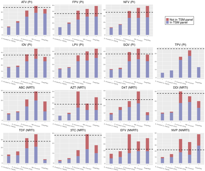
Figure 4: Results on the HIV-1 drug resistance dataset. For each drug class, we plot the number of protease positions (for PI) or reverse transcriptase (RT) positions (for NRTI or NNRTI) selected by different knockoff filters. The color indicates whether or not the selected position appears in the treatment selected mutation (TSM) panel, and the horizontal line shows the total number of positions on the TSM panel.

D.2 Simulations for Robustness

To valid the theoretical findings on robustness, an experiment is provided to illustrate the influence of $n_{1}$ on selection results when the argument follows some unknown Gaussian Graphical model. We set $p=2000$, $n_{2}=1000$ and select $n_{1}$ from $\{100,200,300,400,500,600,700,800,900,1000\}$. After repeating each experiment 30 times, the max number of false discoveries ($\text{FD}_{\max}$), $\text{FDP}_{\max}$, FDR and Power of these simulations are reported in Table 5. It can be observed that $\text{FD}_{\max}$, $\text{FDP}_{\max}$ and FDR can be better controlled with the increase of $n_{1}$, which is consistent with Theorems 4 and 5.

D.3 Full Experimental Results for Power analysis

Full experimental results for power analysis is provided in Tables 6-8. When keeping the $\text{FD}_{\max},\text{FDP}_{\max}$ or FDR under control, we can see that, in most of the settings, a powerful selection result can be made when more samples are added to the second part of dataset. This supports our conclusion in Theorem 6. Indeed, some $\text{FD}_{\max}$ or $\text{FDP}_{\max}$ may exceed the fixed level since $k$-FWER control and FDP control allow errors with a certain probability.

D.4 Experimental Analysis for HIV Dataset

The HIV-1 drug resistance dataset (Rhee et al. 2006) contains data for eight protease inhibitor (PI) drugs, six nucleoside reverse transcriptase inhibitor (NRTI) drugs and four nonnucleoside reverse transcriptase inhibitor (NNRTI) drugs. The response $Y$ is the log-transformed drug resistance level while the feature $X_{j}$ are the markers for the presence or absence of the $j$th mutation (Dai and Barber 2016). Inspired by (Dai and Barber 2016), the drug with high proportion of missing drug resistance measurement are removed (each with over 50% missing data). We only keep those mutations which appear $>10$ times in the sample set, and report the characteristics of resulting dataset in Table 9.

We then apply the E-Knockoff inference associated with Lasso ($2n_{1}=n_{2}=\frac{2n}{3}$), including E-Knockoff ($k$-FWER) ($k=2,\alpha=0.1$), E-Knockoff (FDP) ($q=0.2,\alpha=0.2$), and E-Knockoff (FDR) ($q=0.2$), to these datasets. For comparison, we also apply the Lasso-based MX-Knockoff ($q=0.2$) and DeepPINK ($q=0.2$) to the same data. Figure 4 summaries the selected mutations against the treatment selected mutations (TSM).

Experimental resuts show that E-Knockoff can control the false discovery efficiently for seven PI drugs. Also, the proposed methods would produce many “false discoveries” in NRTI and NNRTI drugs. This may due to the fact that TSM panel may not contain all informative mutations. Similar experimental results are also reported in (Dai and Barber 2016; Lu et al. 2018)

References

- Abadi et al. (2015) Abadi, M.; Agarwal, A.; Barham, P.; Brevdo, E.; Chen, Z.; Citro, C.; Corrado, G. S.; Davis, A.; Dean, J.; Devin, M.; Ghemawat, S.; Goodfellow, I.; Harp, A.; Irving, G.; Isard, M.; Jia, Y.; Jozefowicz, R.; Kaiser, L.; Kudlur, M.; Levenberg, J.; Mané, D.; Monga, R.; Moore, S.; Murray, D.; Olah, C.; Schuster, M.; Shlens, J.; Steiner, B.; Sutskever, I.; Talwar, K.; Tucker, P.; Vanhoucke, V.; Vasudevan, V.; Viégas, F.; Vinyals, O.; Warden, P.; Wattenberg, M.; Wicke, M.; Yu, Y.; and Zheng, X. 2015. TensorFlow: Large-Scale Machine Learning on Heterogeneous Systems. Software available from tensorflow.org.
- Agarap (2018) Agarap, A. F. 2018. Deep Learning using Rectified Linear Units (ReLU). arXiv:1803.08375.
- Bach (2008) Bach, F. 2008. Consistency of the group lasso and multiple kernel learning. Journal of Machine Learning Research, 9(40): 1179 – 1225.
- Bai et al. (2020) Bai, X.; Ren, J.; Fan, Y.; and Sun, F. 2020. KIMI: Knockoff inference for motif identification from molecular sequences with controlled false discovery rate. Bioinformatics, 37(6): 759 – 766.
- Barber and Candès (2015) Barber, R. F.; and Candès, E. J. 2015. Controlling the false discovery rate via knockoffs. Annals of Statistics, 43(5): 2055 – 2085.
- Barber and Candès (2019) Barber, R. F.; and Candès, E. J. 2019. A knockoff filter for high-dimensional selective inference. Annals of Statistics, 47(5): 2504 – 2537.
- Barber, Candès, and Samworth (2020) Barber, R. F.; Candès, E. J.; and Samworth, R. J. 2020. Robust inference with knockoffs. Annals of Statistics, 48(3): 1409 – 1431.
- Benjamini and Hochberg (1995) Benjamini, Y.; and Hochberg, Y. 1995. Controlling the false discovery rate: A practical and powerful approach to multiple testing. Journal of the Royal Statistical Society: Series B (Methodological), 57(1): 289 – 300.
- Benjamini and Yekutieli (2001) Benjamini, Y.; and Yekutieli, D. 2001. The control of the false discovery rate in multiple testing under dependency. The Annals of Statistics, 29(4): 1165 – 1188.
- Buitinck et al. (2013) Buitinck, L.; Louppe, G.; Blondel, M.; Pedregosa, F.; Mueller, A.; Grisel, O.; Niculae, V.; Prettenhofer, P.; Gramfort, A.; Grobler, J.; Layton, R.; VanderPlas, J.; Joly, A.; Holt, B.; and Varoquaux, G. 2013. API design for machine learning software: experiences from the scikit-learn project. In ECML PKDD Workshop: Languages for Data Mining and Machine Learning, 108 – 122.
- Candès et al. (2018) Candès, E. J.; Fan, Y.; Janson, L.; and Lv, J. 2018. Panning for gold: Model-X knockoffs for high-dimensional controlled variable selection. Journal of the Royal Statistical Society: Series B (Statistical Methodology), 80(3): 551 – 577.
- Chen et al. (2021) Chen, H.; Wang, Y.; Zheng, F.; Deng, C.; and Huang, H. 2021. Sparse modal additive model. IEEE Transactions on Neural Networks and Learning Systems, 32(6): 2373 – 2387.
- Christian (2012) Christian, R. 2012. Machine Learning: A Probabilistic Perspective. The MIT Press.
- Dai and Barber (2016) Dai, R.; and Barber, R. F. 2016. The knockoff filter for FDR control in group-sparse and multitask regression. In International Conference on Machine Learning (ICML).
- Delattre and Roquain (2015) Delattre, S.; and Roquain, E. 2015. New procedures controlling the false discovery proportion via Romano-Wolf’s heuristic. The Annals of Statistics, 43(3): 1141 – 1177.
- Efron and Tibshirani (2002) Efron, B.; and Tibshirani, R. 2002. Empirical bayes methods and false discovery rates for microarrays. Genetic Epidemiology, 23(1): 70 – 86.
- Fan, Guo, and Hao (2012) Fan, J.; Guo, S.; and Hao, N. 2012. Variance estimation using refitted cross-validation in ultrahigh dimensional regression. Journal of the Royal Statistical Society: Series B (Statistical Methodology), 74(1): 37 – 65.
- Fan and Li (2001) Fan, J.; and Li, R. 2001. Variable selection via nonconcave penalized likelihood and its oracle properties. Journal of the American Statistical Association, 96(456): 1348 – 1360.
- Fan and Lv (2010) Fan, J.; and Lv, J. 2010. A selective overview of variable selection in high dimensional feature space. Statistica Sinica, 20(1): 101 – 148.
- Fan et al. (2020a) Fan, Y.; Demirkaya, E.; Li, G.; and Lv, J. 2020a. RANK: Large-Scale inference with graphical nonlinear knockoffs. Journal of the American Statistical Association, 115(529): 362 – 379.
- Fan, Demirkaya, and Lv (2019) Fan, Y.; Demirkaya, E.; and Lv, J. 2019. Nonuniformity of p-values can occur early in diverging dimensions. Journal of Machine Learning Research, 20(77): 1 – 33.
- Fan et al. (2020b) Fan, Y.; Lv, J.; Sharifvaghefi, M.; and Uematsu, Y. 2020b. IPAD: Stable interpretable forecasting with knockoffs inference. Journal of the American Statistical Association, 115(532): 1822 – 1834.
- Farcomeni (2008) Farcomeni, A. 2008. A review of modern multiple hypothesis testing, with particular attention to the false discovery proportion. Statistical Methods in Medical Research, 17(4): 347 – 388.
- Frecon, Salzo, and Pontil (2018) Frecon, J.; Salzo, S.; and Pontil, M. 2018. Bilevel learning of the group Lasso structure. In Advances in Neural Information Processing Systems (NeurIPS).
- Friedman, Hastie, and Tibshirani (2010) Friedman, J. H.; Hastie, T.; and Tibshirani, R. 2010. A note on the group lasso and a sparse group lasso. arXiv:1001.0736.
- Genovese and Wasserman (2004) Genovese, C.; and Wasserman, L. 2004. A stochastic process approach to false discovery control. The Annals of Statistics, 32(3): 1035 – 1061.
- Hastie and Tibshirani (1990) Hastie, T. J.; and Tibshirani, R. 1990. Generalized Additive Models. London: Chapman and Hall.
- Hinton and Salakhutdinov (2006) Hinton, G. E.; and Salakhutdinov, R. R. 2006. Reducing the Dimensionality of Data with Neural Networks. Science, 313(5786): 504 – 507.
- Hochberg and Tamhane (1987) Hochberg, Y.; and Tamhane, A. C. 1987. Multiple Comparison Procedures. Wiley.
- Jordon, Yoon, and Mihaela (2019) Jordon, J.; Yoon, J.; and Mihaela, v. d. S. 2019. KnockoffGAN: Generating knockoffs for feature selection using generative adversarial networks. In International Conference on Learning Representations (ICLR).
- Kingma and Ba (2015) Kingma, D. P.; and Ba, J. 2015. Adam: A Method for Stochastic Optimization.
- Korn et al. (2004) Korn, E. L.; Troendle, J. F.; McShane, L. M.; and Simon, R. 2004. Controlling the number of false discoveries: application to high-dimensional genomic data. Journal of Statistical Planning and Inference, 124(2): 379 – 398.