Foothold Evaluation Criterion for Dynamic Transition Feasibility for Quadruped Robots

Abstract

To traverse complex scenarios reliably a legged robot needs to move its base aided by the ground reaction forces, which can only be generated by the legs that are momentarily in contact with the ground. A proper selection of footholds is crucial for maintaining balance. In this paper, we propose a foothold evaluation criterion that considers the transition feasibility for both linear and angular dynamics to overcome complex scenarios. We devise convex and nonlinear formulations as a direct extension of [1] in a receding-horizon fashion to grant dynamic feasibility for future behaviours. The criterion is integrated with a Vision-based Foothold Adaptation (VFA) strategy that takes into account the robot kinematics, leg collisions and terrain morphology. We verify the validity of the selected footholds and the generated trajectories in simulation and experiments with the 90kg quadruped robot HyQ.

I Introduction

Legged robots are versatile machines that make use of their sensors to react, adapt and navigate in complex scenarios. To move, the robot needs to choose a trajectory for the motion of its base, and decide a feasible contact sequence for its feet to follow the base. Motions and contacts need to be both dynamically (e.g., inside the torque limits of the robot’s actuators or not falling) and kinematically feasible (e.g., inside the joints’ range of motion).

Optimization-based techniques for legged robot whole-body control [2, 3, 4, 5] have become prevalent in locomotion, allowing robots to deal with complex terrain. Furthermore, some approaches explicitly include terrain information into the formulation of the locomotion problem [6, 7, 8]. This is possible thanks to advances in state estimation and mapping [9, 10, 11], as well as the algorithmic developments such as the use of automatic differentiation [12] and differential dynamic programming [13, 14]. However, in many cases the introduction of the terrain is not trivial, especially if kinematic and dynamic feasibility are considered. We categorize two main ways to tackle the problem: (a) coupled approaches, in which the base trajectory and footholds are optimized jointly, and (b) decoupled approaches, in which the footholds are selected first and then the trajectory is optimized to follow the footholds.

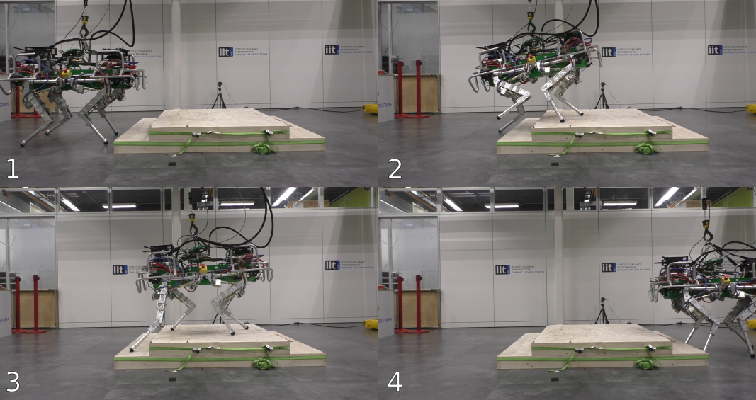
Figure 1: Snapshots of the HyQ robot climbing stair scenario using the proposed foothold evaluation criterion for dynamic transition feasibility.

The main advantage of coupled approaches is that the optimized footholds and trajectories are guaranteed to be realizable by the robot since kinematic and dynamic constraints can be enforced. The main disadvantage is that solving this problem involves a large number of variables and the nature of the problem is in general nonlinear with a large combinatorial space.

Decoupled approaches split the problem in two. The foothold selection can be done heuristically or by solving a less computationally expensive optimization problem. This releases computational load from the main optimization. The disadvantage is that it is difficult to guarantee that the selected footholds yield dynamically feasible trajectory for the robot’s base.

In this paper we try to reach a compromise between these two approaches. We devise a strategy to evaluate if a foothold yields a dynamic transition feasibility for the duration of the stance phase of a leg, coupled with a vision-based foothold selection that reduces the chance of reaching kinematic limits and collisions. We based the evaluation on the Continuous Convex Resolution of Centroidal Dynamic Trajectories (C-CROC), presented in [1]. The method looks for the existence of feasible trajectories for the center of mass (CoM) (parameterized as Bézier curves) according to the single rigid body dynamics model (SRBDM). Additionally, we implement the method presented in [1] to account for the body angular dynamics in a convex (based on the insight provided in [1]) and a nonlinear fashion. We propose and compare the two different formulations to drop the constant angular momentum assumption: one that keeps the convexity of the optimization problem, and a second one that includes the angular dynamics in a nonlinear fashion. We also integrate the Vision-based Foothold Adaptation (VFA) presented in [15] to discard footholds that may lead to collisions or kinematically unreachable locations.

The main contributions are:

1. A dynamic transition feasibility foothold evaluation that considers linear and angular dynamics of the SRBDM. We implemented in simulation and experiments two formulations that consider CoM motion and base orientation; a convex one (based on [1]) that includes angular dynamics without breaking convexity and a novel nonlinear approach.

2. A comparison between a convex and a nonlinear formulation for different scenarios in terms of quality of the generated trajectories.

The paper is organized as follows: Section II summarizes the relevant work; Section III details the formulation of the dynamic transition feasibility and highlights the differences with respect to [1]; in Section IV the two formulations of the optimization problem are presented; simulation and experimental results are presented in Section 5, and in Section VI we address conclusions and future work.

II Related work

We focus on legged locomotion strategies that consider variations on the terrain, making a distinction between coupled and decoupled approaches. Furthermore, we place the work here presented as an intermediate solution between both of these categories.

Coupled approaches control the motion of the robot by formulating a single optimal control problem. This means that the optimization is posed to find a reference (position and orientation) for the body, contact locations (footholds), and inputs (ground reaction forces (GRFs), torques), for a defined planning horizon. One of the most remarkable examples is the one proposed by Winkler et al. [7] which makes the problem more tractable by modeling the robot by means of the SRBDM, although the optimization is still a nonlinear program (NLP). In this case, not only reference trajectories for the body and GRFs are optimized, but also gait timings are included as decision variables. The richness of the optimized motions is demonstrated in complex scenarios. Similar approaches to this were presented previously by solving the optimization problem via sequential linear quadratic (SLQ) [17] and fixing the gait sequence to only optimize timing, posing the problem as a switched system [18]. A different approach is taken by Aceituno et al. [6], where the proposed algorithm computes gait pattern, contact sequence, and CoM trajectories as an outcome of a mixed-integer convex program (MICP) on several convex surfaces. All of the previously mentioned coupled approaches showcase the advantages and the versatility of the generated motions by optimizing inputs, body references and footholds together. However, all of these suffer from large computational times and risk getting stuck in local minima.

Decoupled approaches outsource the foothold selection to an external module. This reliefs computational cost from the optimization, since the foothold positions have a nonlinear relationship with the CoM position [19]. A method that paved the way to account for the terrain was proposed by Kalakrishnan et al. [20], where terrain was discretized considering templates corresponding to portions of the map in the vicinity of a nominal landing position. A linear regression method was used to approximate the selection of an expert user to adapt the landing location of the feet within the template and the motion of the base was designed to follow these footholds. Inspired by this, methods have resourced to template-based foothold selection using learning-based [8, 15, 24, 21, 22, 23] or fast optimization [25, 26] strategies. In this way the optimization problem becomes lighter. The main caveat when selecting footholds prior to the motion is that in general only geometric constraints are considered such as collisions, terrain roughness or kinematic limits. This situation might lead to postures in which the robot is not able to continue the motion due to dynamic infeasibility (e.g., the motion is not achievable due to actuation limits).

Fernbach et al. [1] presented a method to evaluate the transition feasibility of a motion with contact switches. The method relies on the parameterization of the trajectory of the CoM as a Bézier curve, which allows to pose the problem as a quadratic program. The method makes use of the SRBDM. Tsounis et al. [27] used this method to learn dynamic transition feasibility of foothold and devised a learning-based locomotion strategy to generate locomotion in complex scenarios with variable terrain. In a similar line, the authors of [28] trained two coupled neural networks to evaluate the feasibility of the contacts and generate the motion trajectory based on the MICP solved in [6].

We extend the work of [1] to evaluate transition feasibility considering variations of the angular dynamics with both convex and nonlinear formulations, and on the other hand, we use the found trajectory of the CoM and base orientation as reference to guide the base to provide a consistent motion with the transition feasibility metric.

III Formulation of Contact Transition Feasibility with Angular Dynamics

We address the evaluation of dynamic trajectories for the duration of the stance phase of a specific leg. In other words, we want to assert the existence of feasible trajectories in a receding horizon fashion. We generate these trajectories according to the SRBDM considering as a basis the work of [1] and account for the angular dynamics in the optimization. It is worth noticing that in [1], a theoretical implementation of $\dot{\mathbf{L}}\neq 0$ is discussed. We propose in the next sections two ways to address this consideration.

We follow the same argument given in [1], which is to connect two different sets of states in space and time, we include angular quantities to the set of states. Thus, a state is defined as ${\mathbf{x}(t)=[\mathbf{c}(t)\;\mathbf{\dot{c}}(t)\;\mathbf{\ddot{c}}(t)\;\bm{\Theta}(t)\;\dot{\bm{\Theta}}(t)\;\ddot{\bm{\Theta}}(t)]^{\intercal}\in\mathbb{R}^{6\times 3}}$, where $\mathbf{c}$ is the position of the CoM and $\bm{\Theta}$ is the orientation of the base, expressed in terms of roll ($\phi$), pitch ($\gamma$) and yaw ($\psi$) angles.

A feasible dynamic transition subject to dynamics constraints that connects two sets of states is defined as ${\bm{f}(t):\mathbf{x}(t_{0})\rightarrow\mathbf{x}(t_{f}),\;t_{f}>t_{0}}$, where $t_{0}$ and $t_{f}$ correspond to the initial and final states respectively. We employ continuously differentiable, parametric curves to describe position and orientation (similarly to [1]) to reduce the number of decision variables.

III-A Time horizon description

We choose to express the considered time horizon in terms of contact switches to have a general description, applicable to any type of gait. A contact switch happens whenever any foot makes or breaks a contact with the ground. We define a contact switch horizon (CSH) as the number of non-simultaneous contact switches occurring in the considered period $T=t_{f}-t_{0}$.

Figure 2: Example of sub-horizon partitioning. The CoM trajectory connecting the initial ($\mathbf{x}_{0}$) and the final ($\mathbf{x}_{f}$) states is partitioned into multiple sub-horizons. Each of them is labeled according to an increasing index $i$ and is subject to a different set of constraints.

Once a desired evaluation time horizon is chosen, we compute the CSH assuming a periodic gait. A similar approach has been adopted in [1], where the trajectory is split at contact switches, to consider transitions between different phases.

For the sake of completeness, we provide a brief description of the method presented in [1] pointing out the main differences with respect to what is presented here. In [1], Bézier curves are adopted to describe the CoM trajectory. They are curves parametrized by control points. Thanks to the properties of Bézier curves, one can ensure that the generated continuous trajectories remain within the constraints. In [1], it is mentioned that the number of contact switches can be increased arbitrarily. However, in our experience, we faced feasibility problems since the method generates a single Bézier curve for the entire horizon (with multiple contact switches) with only one degree of freedom (a single free moving control point). The solution space of feasible trajectories is thus reduced as the number of contact switches increases, since the number of constraints increases. To prevent such reduction, we adopt a CSH partitioning method (sub-horizon, Fig. 2). We choose to limit each sub-horizon to two contact switches to prevent the reduction of the solution space. Such limit is specifically chosen to connect two sub-sequent stance phases, i.e., lift-off and touchdown of the same leg. Then, to evaluate an arbitrarily large CSH, we concatenate multiple sub-horizons by means of continuity constraints. This leads to a set of parametric curves, one curve for each sub-horizon, chained together at way-points (connection points between sub-curves) to evaluate a longer CSH.

We adopt the SRBDM to assert dynamic transition feasibility:

$$\underbrace{\begin{bmatrix}m(\ddot{\mathbf{c}}-\mathbf{g})\\ m\mathbf{c}\times(\ddot{\mathbf{c}}-\mathbf{g})+\dot{\mathbf{L}}\end{bmatrix}}_{\mathbf{w}}=\underbrace{\begin{bmatrix}\mathbf{I}_{3}&\ldots&\mathbf{I}_{3}\\ [\mathbf{p}_{1}]_{\times}&\ldots&[\mathbf{p}_{j}]_{\times}\end{bmatrix}}_{\mathbf{A}}\mathbf{f}$$ (1)

where $\mathbf{g}$ is the gravity vector, $\mathbf{I}_{3}\in\mathbb{R}^{3\times 3}$ is the identity matrix, $\mathbf{f}=[\mathbf{f}_{1}\text{ }\ldots\text{ }\mathbf{f}_{j}]^{\intercal}$, $\mathbf{f}_{j}\in\mathbb{R}^{3}$ is the ground reaction force (GRF) associated to the j^th at point $\mathbf{p}_{j}\in\mathbb{R}^{3}$ expressed in the world frame and $m$ is the robot’s mass. We express $\dot{\mathbf{L}}$ as a function of the angular quantities (orientation, rate and acceleration) by analytically differentiating $\mathbf{L}=\mathbf{I}_{\mathcal{W}}\bm{\upomega}$, where $\bm{\upomega}$ is angular velocity of the rigid body expressed in the CoM frame. One can express $\bm{\upomega}$ in terms of $\dot{\bm{\Theta}}$ making use of the following mapping:

$$\bm{\upomega}=\mathbf{T}(\gamma,\psi)\dot{\mathbf{\Theta}}$$ (2)

where the matrix $\mathbf{T}$ is the matrix that maps angular velocity in the world frame to rotation rates. The derivative of $\mathbf{L}$ is given by:

$$\dot{\mathbf{L}}= \underbrace{\mathbf{T}\bm{\dot{\Theta}}\times\mathbf{I}_{\mathcal{W}}\mathbf{T}\dot{\bm{\Theta}}}_{\dot{\mathbf{I}}_{\mathcal{W}}\bm{\upomega}}+\underbrace{\mathbf{I}_{\mathcal{W}}\cdot(\dot{\mathbf{T}}\dot{\bm{\Theta}}+\mathbf{T}\ddot{\bm{\Theta}})}_{\mathbf{I}_{\mathcal{W}}\dot{\bm{\upomega}}}$$ (3)

Note that (3) is a highly nonlinear expression that depends on $\bm{\Theta}$ and its derivatives.

In the following section we describe the two proposed formulations (convex and nonlinear) to solve the dynamic transition feasibility problem while accounting for the rate of change of angular momentum $\dot{\mathbf{L}}$. The first formulation aims at preserving the convexity of the problem, thus making it computationally efficient and not prone to local minima, at the cost of a more limited solution space. The second formulation offers a wider solution space with more computational cost.

IV Solution of Contact Transition Feasibility with Angular Dynamics

In this section, we describe two formulations to solve the transition feasibility problem, namely the convex and the nonlinear approaches. In the convex approach, we overcome the nonconvexity of the $\dot{\mathbf{L}}$ analytical expression by decoupling the linear and the angular parts and including $\dot{\mathbf{L}}$ as an optimization variable. This formulation yields a more limited solution space with respect to the nonlinear one. This is because the intermediate points in the CSH are fixed, whereas in the nonlinear case we allow variations of the intermediate and final desired states, as shown in Fig. 3. To do so (3) as a constraint in function of angular quantities ($\bm{\Theta}$, $\dot{\bm{\Theta}}$, $\ddot{\bm{\Theta}}$) which are now included as decision variables, leading to smoother and more versatile motions.

To produce consistent solutions, we include boundary constraints in our formulation. We define a pair of initial and final states associated to an i^th sub-horizon $\mathbf{x}_{0,\;i}$, $\mathbf{x}_{f,\;i}$ (Fig. 2). $\mathbf{x}_{0,\;i}=\mathbf{x}_{f,\;i-1}$ is the definition of a continuous function. We can write this relationship for every sub-horizon as:

$$\left[\begin{matrix}\mathbf{x}_{0,\;2}&\mathbf{x}_{0,\;3}&\ldots&\mathbf{x}_{0,\;i}\end{matrix}\right]^{\intercal} =\left[\begin{matrix}\mathbf{x}_{f,\;1}&\mathbf{x}_{f,\;2}&\ldots&\mathbf{x}_{f,\;i-1}\end{matrix}\right]^{\intercal}$$

$$\mathbf{X}_{0} =\mathbf{X}_{f}$$ (4)

This relationship is implicitly valid for all the sub-horizons in the convex formulation because of predefined states, but in the nonlinear case it has to be explicitly enforced.

IV-A Convex formulation

Figure 3: Example of convex (left) and nonlinear (right) CoM linear trajectories. The CSH is divided in different parts with their own set of constraints. The initial ($\mathbf{c}_{0}$), final ($\mathbf{c}_{f}$) and intermediate positions have to be defined a priori in the convex case, while in the nonlinear one they are optimized. The solid black circles are the computed states, while the blue dashed circles are the desired states before the corrective action of the nonlinear optimization.

For each sub-horizon we parameterize the CoM trajectory with an 8^th order Bézier curve to define the trajectory up to its third analytical derivative. A generic n^th order Bézier curve has $(n+1)$ control points and each can be associated to a different state quantity (position, velocity and acceleration). We then leave a free control point per each sub-curve. The collected points are used as optimization variables ($\bm{\uprho}$) and the system dynamics are described as

$$\underbrace{\begin{bmatrix}m(\ddot{\mathbf{c}}(\bm{\uprho})-\mathbf{g})\\ m\mathbf{c}(\bm{\uprho})\times(\ddot{\mathbf{c}}(\bm{\uprho})-\mathbf{g})+\dot{\mathbf{L}}\end{bmatrix}}_{\mathbf{w}(\bm{\uprho})} =\underbrace{\begin{bmatrix}\mathbf{I}_{3}&\ldots&\mathbf{I}_{3}\\ [\mathbf{p}_{1}]_{\times}&\ldots&[\mathbf{p}_{j}]_{\times}\end{bmatrix}}_{\mathbf{A}}\mathbf{f}$$

$$\mathbf{w}(\bm{\uprho}) =\mathbf{A}\mathbf{f}$$ (5)

where $\bm{\uprho}\in\mathbb{R}^{i\times 3}$ is the collection of free control points associated to each sub-horizon (Fig. 2). Although the term $\mathbf{c}(\bm{\uprho})\times\ddot{\mathbf{c}}(\bm{\uprho})$ is a nonlinear term, it can be shown that it can be formulated as a linear constraint by employing Bézier curves to describe the CoM trajectory $\mathbf{c}$ [1].

To include the angular momentum rate $\dot{\mathbf{L}}$ preserving convexity, we define $\dot{\mathbf{L}}$ as an optimization variable and compute a desired $\dot{\mathbf{L}}_{ref}$, which is then tracked by including the term $\parallel\mathbf{\dot{L}}-\mathbf{\dot{L}}_{ref}\parallel^{2}_{2}$ in the cost function. To compute $\dot{\mathbf{L}}_{ref}$, we define a desired angular behaviour of the robot by designing a trajectory for the angular variables ($\bm{\Theta}$, $\dot{\bm{\Theta}}$, $\ddot{\bm{\Theta}}$) and then computing the angular momentum rate with the full expression (3). In the convex case, we decide to describe the trajectory of the desired $\bm{\Theta}$ as a Bézier curve, to keep a finite number of parameters. We then formulate the optimization problem as:

$$\!{\bm{\min}_{{\bm{\uprho},\mathbf{f},\dot{\mathbf{L}}}}} \displaystyle\sum_{k=0}^{N\cdot i} \parallel\mathbf{\dot{L}}_{k}-\mathbf{\dot{L}}_{ref,\;k}\parallel_{2}^{2}+\parallel\ddot{\mathbf{c}}_{k}(\bm{\uprho}_{i})\parallel_{2}^{2}$$

subject to $$\mathbf{w}_{k}(\bm{\uprho}_{i})=\mathbf{A}_{k}\mathbf{f}_{k}$$ (6a)

$$0\;\leq f_{z,\;k}\;\leq f_{max}$$ (6b)

$$|f_{x,\;k}|\leq\mu f_{z,\;k},\quad|f_{y,\;k}|\leq\mu f_{z,\;k}$$ (6c)

where $f_{max}$ is an upper limit for the $z$ direction of the force that the robot can exert on the ground. The tracking cost for the desired angular momentum rate is given by $\parallel\mathbf{\dot{L}}-\mathbf{\dot{L}}_{ref}\parallel_{2}^{2}$ and we minimize the accelerations ($\parallel\ddot{\mathbf{c}}(\bm{\uprho})\parallel_{2}^{2}$) to incentivize smoother trajectories. This first method of including $\dot{\mathbf{L}}\neq 0$ differs from [1] since we are not directly including $\dot{\mathbf{L}}$ as a parametric curve, but rather expressing $\dot{\mathbf{L}}$ as a function of a desired angular trajectory.

IV-B Nonlinear formulation

We present an alternative formulation to the one presented in Section IV-A. The main difference is that herein we aim to directly optimize the trajectories of the angular quantities along the CSH, instead of using them as parameters to generate and track a desired $\dot{\mathbf{L}}$. One of the main advantages of this approach is that this method does not require to set extra constraints to maintain physical consistency. In particular we introduced slack variables on the position and acceleration of the intermediate and final states, keeping fixed the velocity to reach the commanded velocity at each way-point (Fig. 3). This makes the problem nonlinear due to the dependency of $\dot{\mathbf{L}}$ with respect to the angular position, velocity and acceleration. We then define a set of enhanced states as $\overline{\mathbf{x}}=\mathbf{x}_{d}+\mathbf{x}_{v}$, composed by a desired $\mathbf{x}_{d}=\left[\begin{matrix}\mathbf{c}_{d}&\dot{\mathbf{c}}_{d}&\ddot{\mathbf{c}}_{d}&\bm{\Theta}_{d}&\dot{\bm{\Theta}}_{d}&\ddot{\bm{\Theta}}_{d}\end{matrix}\right]^{\intercal}$ and a variable ${\mathbf{x}_{v}=\left[\begin{matrix}\Delta\mathbf{c}&0&\Delta\ddot{\mathbf{c}}&0&0&0\end{matrix}\right]^{\intercal}}$ part,

Figure 4: Locomotion control pipeline used to implement the proposed foothold evaluation strategies in both experiments and simulations.

where ${\Delta\mathbf{c}\in\mathbb{R}^{3}}$ and $\Delta\ddot{\mathbf{c}}_{v}\in\mathbb{R}^{3}$ are decision variables.

We consider velocity and position/orientation variables as commanded quantities. Although they are not enhanced, they are still allowed to vary in between user-defined states in order to reach the designated value at each way-point while fulfilling the imposed constraints. The optimization problem is then built as follows:

$$\!{\bm{\min}_{{\bm{\uprho},\mathbf{f},\Delta\mathbf{c},\Delta\ddot{\mathbf{c}},\bm{\Theta},\dot{\bm{\Theta}},\ddot{\bm{\Theta}}}}} \displaystyle\sum_{k=0}^{N\cdot i}\parallel\dot{\mathbf{L}_{k}}\parallel_{2}^{2}+\parallel\ddot{\mathbf{c}}_{k}(\bm{\uprho}_{i},\;\Delta\ddot{\mathbf{c}}_{i})\parallel_{2}^{2}$$ (7a)

subject to $$\mathbf{w}_{k}(\bm{\uprho}_{i},\Delta\mathbf{c}_{i},\Delta\ddot{\mathbf{c}}_{i})=\mathbf{A}_{k}\mathbf{f}_{k}$$ (7b)

$${\dot{\mathbf{L}}_{k}=\dot{\mathbf{L}}_{f}(\bm{\Theta}_{k},\dot{\bm{\Theta}}_{k},\ddot{\bm{\Theta}}_{k})}$$ (7c)

$$\mathbf{X}_{0}=\mathbf{X}_{f}$$ (7d)

$$0\;\leq f_{z,\;k}\;\leq f_{max}$$ (7e)

$$|f_{x,\;k}|\leq\mu f_{z,\;k},\quad|f_{y,\;k}|\leq\mu f_{z,\;k}$$ (7f)

where the cost function is similar to the one adopted in the convex formulation. The main difference consists in $\parallel\dot{\mathbf{L}_{k}}\parallel_{2}^{2}$, which is a cost term that aims at reducing the angular variation rather than tracking a reference behavior, helping to incentivize less aggressive motions for the angular quantities. We then consider (3) as a constraint dependent in the angular quantities defined as $\dot{\mathbf{L}}_{f}(\bm{\Theta},\dot{\bm{\Theta}},\ddot{\bm{\Theta}})$ and account for these quantities as decision variables. This formulation is computationally more expensive than the convex formulation and it is prone to local minima, but the output trajectories are qualitatively better compared to the convex formulation solutions.

V Results

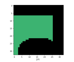
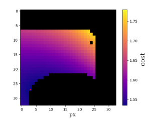
Figure 5: Comparison of VFA (terrain roughness, kinematic reachability, collisions) versus dynamic foothold evaluation for the RF foot during stair climbing. In the case of the VFA evaluation, green pixels indicate safe landing locations and black unsafe. For the dynamic evaluation black pixels are dynamically infeasible footholds and we show the cost from the solution of (7a) indicated by the colorbar.

In this section we evaluate the proposed evaluation criterion and the two proposed formulations. We show an example of an evaluation of a series of contact locations for foothold selection and verify the feasibility of the generated trajectories in a stair climbing scenario. Additional results on flat terrain are reported in the accompanying video.

V-A Implementation details

To verify the feasiblity of the generated trajectories provided by the foothold evaluation, we adopt the control scheme shown in Fig. 4. The Foothold Reference Generator (FRG) is in charge of generating the foothold positions with respect to the actual CoM’s states and foothold positions ($\mathbf{x}_{act}$, $\mathbf{p}_{act}$), according to the user commanded velocity. The reference foothold positions are evaluated with the VFA [15], which discards unsuitable footholds according to geometric constraints and sends the adapted foothold positions $\mathbf{p}^{*}\in\mathbb{R}^{nc\times 3}$ to both the Dynamic Optimizer and IK blocks, for all the contact points $nc$. The Dynamic Optimizer block encapsulates the methods presented in this paper. Given the set of the actual states, the adapted footholds and the user command, it generates the state references that will be provided to both the inverse kinematics (IK) block and the whole-body controller (WBC) [29]. The IK computes the joint positions and velocities, providing the whole-body control (WBC) with a set of joint references for the swing leg trajectories. The WBC computes the required GRFs to track the reference quantities, transforming them into joint torques. They are then commanded to the low-level control, which is in charge of performing the joint torque control.

The convex formulation makes use of the CVXPY modeling language [30, 31], with ECOS [32] as solver. The nonlinear approach relies on CasADi [33], acting as an interface with IPOPT [34]. We evaluated our methods in simulation and experiments. The simulations were performed on a i7-8700 CPU using Gazebo [35]. In the experimental setup, we execute the optimization on an off-board computer. The generated reference is sent to the onboard Control computer via ROS messages [36]. In the case of the simulations, we assume no computational time constraints to visualize the behavior of the robot while executing the generated trajectories, whereas in the experiment we perform a new optimization at each step due to the time constraints of the approach.

V-B Foothold Dynamic Feasibility Evaluation

Figure 6: Comparison between angular rates (pitch rate) in simulated stairs scenario. The solid blue line is the pitch rate traversing the scenario considering $\dot{\mathbf{L}}=0$, while the solid red line is the angular velocity achieved using our nonlinear approach, where $\dot{\mathbf{L}}\neq 0$.

We evaluate the dynamic transition feasiblity on a stair climbing scenario. We compute a set of nominal future foothold locations assuming a periodic gait during one gait cycle. We then evaluate the neighboring area of the nominal footholds to avoid reaching kinematic limits, collisions or unsafe landing locations using the VFA [15]. Subsequently, we check if there exists a trajectory that solves the problem formulated in (7a) for every candidate foothold. If the solution exists, the foothold is deemed dynamically feasible. Additionally we compute a cost map to visualize the ”quality” of the solution provided by each candidate foothold. Fig. 5 shows an example of evaluated candidate footholds for the RF leg during a crawl while climbing stairs. Each pixel in the figure represents a candidate landing location. It can be seen that in the dynamic evaluation (Fig. 5 on the right) the footholds located on the top right corner of the area yield a higher cost, and some footholds deemed feasible using the VFA (Fig. 5 on the left) are discarded since no feasible trajectories to solve (7a) was found.

V-C Simulations

Effect of time varying angular momentum.

We highlight the importance of considering $\dot{\mathbf{L}}\neq 0$. Fig. 6 shows a comparison of the pitch velocity for the case where $\dot{\mathbf{L}}=0$ and $\dot{\mathbf{L}}\neq 0$. Both of these while climbing stairs using the nonlinear formulation. It can be noted that in the case of $\dot{\mathbf{L}}=0$ the peaks in velocity are considerably larger. The same simulation applying the convex version of the approach yielded similar results, which are omitted for the sake of brevity. These results highlight the importance of the angular dynamics when dealing with rough terrain.

Figure 7: Simulation on stairs. The dashed and solid blue lines are the nonlinear reference and tracking, respectively. The dashed and solid red lines are the convex reference and tracking, respectively. Pitch reference and tracking (third row) follow the same color code as linear quantities. In the last row an example of feet trajectories is shown, where LF:Left Front, RF:Right Front, LH:Left Hind, and RH:Right Hind.

Comparison between convex and nonlinear formulation.

Fig. 7 shows a comparison of the executed trajectories and their reference for both the convex and nonlinear formulation in a stair climbing scenario. Although both approaches are able to go up and down the stairs, looking closely at the generated trajectory in the $xy$ plane, one can see that the nonlinear trajectory yields less aggressive changes of direction compared to its convex counterpart. Looking at the velocity in the $y$ direction it can be seen that the amplitude of the variation of the reference and the executed velocity is always larger in the case of the convex formulation with respect to the nonlinear one. We also provide a comparison between the two approaches on flat terrain in the accompanying video to highlight that even on a simple scenario the nonlinear formulation provides smoother trajectories with less peaks in velocity. Regarding computation times, the convex took 2.90s for the stair scenario and 2.96s for the flat scenario in average over multiple trials to solve the optimization problem, whereas the nonlinear formulation takes 12.78s for the stair scenario and 8.0s for the flat scenario.

V-D Experiments

Figure 8: Stairs experiment with nonlinear approach. For the top two plots, dashed lines are reference and solid lines are tracking signal. The top plot shows the CoM trajectory tracking on the $xy$ plane and the middle plot shows the pitch tracking. On the last row we show the feet trajectories, where LF:Left Front, RF:Right Front, LH:Left Hind, and RH:Right Hind.

In this section we evaluate the hardware feasibility of the optimized trajectories on the quadruped robot HyQ. We decided to test the trajectory generated by the nonlinear formulation since it is the one that proved better in terms of generated trajectories. The scenario tested is shown in the snapshots of Fig. 1. It consists of climbing and descending two steps of 8cm each. Fig. 8 shows the tracking of the CoM trajectory on the $xy$ plane and the pitch of the robot. As it can be seen, the robot is able to cross the scenario with a low tracking error in both position and orientation. As in the case of the simulation, the accompanying video shows an experiment of the robot executing the optimized trajectories on flat terrain and stairs.

VI Conclusions

We presented a foothold evaluation criterion to assess the existence of dynamically feasible trajectories for legged locomotion that considers both linear and angular dynamics. We extended the method in [1] by formulating the problem allowing variations in the angular momentum along the trajectory (i.e., $\dot{\mathbf{L}}\neq 0$) as a function of a desired angular trajectory. We presented two different formulations (a convex and a nonlinear) both able to generate feasible CoM trajectories. We showed that the convex formulation is faster to compute (4 times in average faster than the nonlinear) and not subject to local minima, while its nonlinear counterpart is able to generate smoother trajectories.

When dealing with less dynamic gaits, such as crawl, the robot can track any desired linear and angular behaviour. But when more dynamic gaits are considered (e.g., trot), the optimization problem might not be able to find a solution due to the inability to track linear and angular quantities simultaneously because of underactuation. Not being able to forecast how close the solution will be to the reference $\dot{\mathbf{L}}_{ref}$ in the convex formulation, may lead to unforeseen consequences in terms of tracking and trajectory generation. This would require to bound $\dot{\mathbf{L}}$ between physically meaningful limits (e.g. the maximum moment that the robot can counteract), which is out of the scope of this paper.A key limitation that affects future implementations of the convex formulation is the need of designing constraints to limit the value $\dot{\mathbf{L}}$ to be physically achievable given actuators limits. In the case of both approaches, the computation times do not allow them to be used continuously to assess footholds and provide CoM reference online.

As future work we aim to extend the proposed formulations to include more dynamic gaits, such as trot, and to design a learning algorithm that is able to approximate the proposed formulations, reducing computational burden.

References

- [1] P. Fernbach, S. Tonneau, O. Stasse, J. Carpentier, and M. Taïx, “C-croc: Continuous and convex resolution of centroidal dynamic trajectories for legged robots in multicontact scenarios,” IEEE Transactions on Robotics, vol. 36, no. 3, pp. 676–691, 2020.
- [2] S. Kuindersma, R. Deits, M. Fallon, A. Valenzuela, H. Dai, F. Permenter, T. Koolen, P. Marion, and R. Tedrake, “Optimization-based locomotion planning, estimation, and control design for the atlas humanoid robot,” Autonomous Robots, vol. 4, no. 40, pp. 429–455, March 2016.
- [3] D. Kim, J. Lee, J. Ahn, O. Campbell, H. Hwang, and L. Sentis, “Computationally-robust and efficient prioritized whole-body controller with contact constraints,” in IEEE/RSJ International Conference on Intelligent Robots and Systems (IROS), October 2018, pp. 1–8. [Online]. Available: https://doi.org/10.1109/IROS.2018.8593767
- [4] J. Di Carlo, P. M. Wensing, B. Katz, G. Bledt, and S. Kim, “Dynamic Locomotion in the MIT Cheetah 3 Through Convex Model-Predictive Control,” in 2018 IEEE/RSJ International Conference on Intelligent Robots and Systems (IROS), October 2018, pp. 1–9. [Online]. Available: https://doi.org/10.1109/IROS.2018.8594448
- [5] S. Fahmi, C. Mastalli, M. Focchi, and C. Semini, “Passive whole-body control for quadruped robots: Experimental validation over challenging terrain,” IEEE Robotics and Automation Letters, vol. 4, no. 3, pp. 2553–2560, July 2019. [Online]. Available: https://doi.org/10.1109/LRA.2019.2908502
- [6] B. Aceituno-Cabezas, C. Mastalli, H. Dai, M. Focchi, A. Radulescu, D. G. Caldwell, J. Cappelletto, J. C. Grieco, G. Fernández-López, and C. Semini, “Simultaneous contact, gait, and motion planning for robust multilegged locomotion via mixed-integer convex optimization,” IEEE Robotics and Automation Letters, vol. 3, no. 3, pp. 2531–2538, July 2018. [Online]. Available: https://doi.org/10.1109/LRA.2017.2779821
- [7] A. W. Winkler, C. D. Bellicoso, M. Hutter, and J. Buchli, “Gait and trajectory optimization for legged systems through phase-based end-effector parameterization,” IEEE Robotics and Automation Letters, vol. 3, no. 3, pp. 1560–1567, July 2018. [Online]. Available: https://doi.org/10.1109/LRA.2018.2798285
- [8] O. Villarreal, V. Barasuol, P. M. Wensing, D. G. Caldwell, and C. Semini, “Mpc-based controller with terrain insight for dynamic legged locomotion,” in 2020 IEEE International Conference on Robotics and Automation (ICRA), 2020, pp. 2436–2442.
- [9] S. Nobili, M. Camurri, V. Barasuol, M. Focchi, D. Caldwell, C. Semini, and M. Fallon, “Heterogeneous sensor fusion for accurate state estimation of dynamic legged robots,” in Proceedings of Robotics: Science and Systems, Cambridge, Massachusetts, July 2017. [Online]. Available: https://doi.org/10.15607/RSS.2017.XIII.007
- [10] T. Flayols, A. Del Prete, P. Wensing, A. Mifsud, M. Benallegue, and O. Stasse, “Experimental evaluation of simple estimators for humanoid robots,” in 2017 IEEE-RAS 17th International Conference on Humanoid Robotics (Humanoids), 2017, pp. 889–895.
- [11] P. Fankhauser and M. Hutter, “A Universal Grid Map Library: Implementation and Use Case for Rough Terrain Navigation,” in Robot Operating System (ROS) - The Complete Reference (Volume 1), A. Koubaa, Ed. Springer, February 2016, ch. 5. [Online]. Available: https://doi.org/10.1007/978-3-319-26054-9_5
- [12] M. Giftthaler, M. Neunert, M. Stäuble, M. Frigerio, C. Semini, and J. Buchli, “Automatic differentiation of rigid body dynamics for optimal control and estimation,” Advanced Robotics, vol. 31, no. 22, pp. 1225–1237, November 2017. [Online]. Available: https://doi.org/10.1080/01691864.2017.1395361
- [13] D. Mayne, “A second-order gradient method for determining optimal trajectories of non-linear discrete-time systems,” International Journal of Control, vol. 3, no. 1, pp. 85–95, 1966. [Online]. Available: https://doi.org/10.1080/00207176608921369
- [14] H. Li and P. M. Wensing, “Hybrid systems differential dynamic programming for whole-body motion planning of legged robots,” IEEE Robotics and Automation Letters, vol. 5, no. 4, pp. 5448–5455, 2020.
- [15] O. Villarreal, V. Barasuol, M. Camurri, L. Franceschi, M. Focchi, M. Pontil, D. G. Caldwell, and C. Semini, “Fast and continuous foothold adaptation for dynamic locomotion through cnns,” IEEE Robotics and Automation Letters, pp. 1–1, 2019.
- [16] C. Semini, N. G. Tsagarakis, E. Guglielmino, M. Focchi, F. Cannella, and D. G. Caldwell, “Design of hyq - a hydraulically and electrically actuated quadruped robot,” IMechE Part I: Journal of Systems and Control Engineering, vol. 225, no. 6, pp. 831–849, 2011.
- [17] M. Neunert, F. Farshidian, A. W. Winkler, and J. Buchli, “Trajectory Optimization Through Contacts and Automatic Gait Discovery for Quadrupeds,” IEEE Robotics and Automation Letters, vol. 2, no. 3, pp. 1502–1509, 2017.
- [18] F. Farshidian, M. Neunert, A. W. Winkler, G. Rey, and J. Buchli, “An efficient optimal planning and control framework for quadrupedal locomotion,” in 2017 IEEE International Conference on Robotics and Automation (ICRA), 2017, pp. 93–100.
- [19] D. Orin, A. Goswami, and S.-H. Lee, “Centroidal Dynamics of a Humanoid Robot,” Autonomous Robots, vol. 35, 10 2013.
- [20] M. Kalakrishnan, J. Buchli, P. Pastor, and S. Schaal, “Learning locomotion over rough terrain using terrain templates,” in 2009 IEEE/RSJ International Conference on Intelligent Robots and Systems, 2009, pp. 167–172.
- [21] V. Barasuol, M. Camurri, S. Bazeille, D. G. Caldwell, and C. Semini, “Reactive trotting with foot placement corrections through visual pattern classification,” in 2015 IEEE/RSJ International Conference on Intelligent Robots and Systems (IROS), September 2015, pp. 5734–5741. [Online]. Available: https://doi.org/10.1109/IROS.2015.7354191
- [22] D. Belter, J. Bednarek, H. Lin, G. Xin, and M. Mistry, “Single-shot Foothold Selection and Constraint Evaluation for Quadruped Locomotion,” in 2019 International Conference on Robotics and Automation (ICRA), 2019, pp. 7441–7447.
- [23] L. Chen, S. Ye, C. Sun, A. Zhang, G. Deng, T. Liao, and J. Sun, “CNNs based Foothold Selection for Energy-Efficient Quadruped Locomotion over Rough Terrains,” in 2019 IEEE International Conference on Robotics and Biomimetics (ROBIO), 2019, pp. 1115–1120.
- [24] D. Esteban, O. Villarreal, S. Fahmi, C. Semini, and V. Barasuol, “On the Influence of Body Velocity in Foothold Adaptation for Dynamic Legged Locomotion via CNNs,” in International Conference on Climbing and Walking Robots (CLAWAR), Moscow, Russia, Aug. 2020, accepted, pp. 353–360.
- [25] P. Fankhauser, M. Bjelonic, C. Dario Bellicoso, T. Miki, and M. Hutter, “Robust Rough-Terrain Locomotion with a Quadrupedal Robot,” in 2018 IEEE International Conference on Robotics and Automation (ICRA), 2018, pp. 5761–5768.
- [26] F. Jenelten, T. Miki, A. E. Vijayan, M. Bjelonic, and M. Hutter, “Perceptive Locomotion in Rough Terrain – Online Foothold Optimization,” IEEE Robotics and Automation Letters, vol. 5, no. 4, pp. 5370–5376, 2020.
- [27] V. Tsounis, M. Alge, J. Lee, F. Farshidian, and M. Hutter, “Deepgait: Planning and control of quadrupedal gaits using deep reinforcement learning,” IEEE Robotics and Automation Letters, vol. 5, no. 2, pp. 3699–3706, 2020.
- [28] Y. Lin, B. Ponton, L. Righetti, and D. Berenson, “Efficient Humanoid Contact Planning using Learned Centroidal Dynamics Prediction,” in 2019 International Conference on Robotics and Automation (ICRA), 2019, pp. 5280–5286.
- [29] M. Focchi, A. del Prete, I. Havoutis, R. Featherstone, D. G. Caldwell, and C. Semini, “High-slope terrain locomotion for torque-controlled quadruped robots,” Autonomous Robots, vol. 41, no. 1, pp. 259–272, 2017. [Online]. Available: http://dx.doi.org/10.1007/s10514-016-9573-1
- [30] S. Diamond and S. Boyd, “CVXPY: A Python-embedded modeling language for convex optimization,” Journal of Machine Learning Research, vol. 17, no. 83, pp. 1–5, 2016.
- [31] A. Agrawal, R. Verschueren, S. Diamond, and S. Boyd, “A rewriting system for convex optimization problems,” Journal of Control and Decision, vol. 5, no. 1, pp. 42–60, 2018.
- [32] A. Domahidi, E. Chu, and S. Boyd, “ECOS: An SOCP solver for embedded systems,” in European Control Conference (ECC), 2013, pp. 3071–3076.
- [33] J. A. E. Andersson, J. Gillis, G. Horn, J. B. Rawlings, and M. Diehl, “CasADi – A software framework for nonlinear optimization and optimal control,” Mathematical Programming Computation, vol. 11, no. 1, pp. 1–36, 2019.
- [34] L. T. B. A. Wächter, “On the implementation of a primal-dual interior point filter line search algorithm for large-scale nonlinear programming,” Mathematical Programming, vol. 106, no. 1, pp. 25–57, 2006.
- [35] N. Koenig and A. Howard, “Design and use paradigms for gazebo, an open-source multi-robot simulator,” in 2004 IEEE/RSJ International Conference on Intelligent Robots and Systems (IROS) (IEEE Cat. No.04CH37566), vol. 3, 2004, pp. 2149–2154 vol.3.
- [36] A. Koubaa, Robot Operating System (ROS): The Complete Reference (Volume 1), 1st ed. Springer Publishing Company, Incorporated, 2016.