Variational Inference with Locally Enhanced Bounds for Hierarchical Models

Abstract

Hierarchical models represent a challenging setting for inference algorithms. MCMC methods struggle to scale to large models with many local variables and observations, and variational inference (VI) may fail to provide accurate approximations due to the use of simple variational families. Some variational methods (e.g. importance weighted VI) integrate Monte Carlo methods to give better accuracy, but these tend to be unsuitable for hierarchical models, as they do not allow for subsampling and their performance tends to degrade for high dimensional models. We propose a new family of variational bounds for hierarchical models, based on the application of tightening methods (e.g. importance weighting) separately for each group of local random variables. We show that our approach naturally allows the use of subsampling to get unbiased gradients, and that it fully leverages the power of methods that build tighter lower bounds by applying them independently in lower dimensional spaces, leading to better results and more accurate posterior approximations than relevant baselines.

1 Introduction

Hierarchical models (Kreft & De Leeuw, 1998; Gelman, 2006; Snijders & Bosker, 2011) represent a general class of probabilistic models which are used in a wide range of scenarios. They have been successfully applied in psychology (Vallerand, 1997), ecology (Royle & Dorazio, 2008; Cressie et al., 2009), political science (Lax & Phillips, 2012), collaborative filtering (Lim & Teh, 2007), and topic modeling (Blei et al., 2003), among others. While these models may take a wide range of forms, a widely used one consists of a tree structure, where a set of global variables $\theta$ controls the distribution over local variables $z_{i}$ in multiple independent groups (see Figure 1 (left)). Then, after observing some data $y_{i}$ from each group, the inference problem consists in accurately approximating the posterior distribution over the global and local variables.

Figure 1: Tighter bounds using importance weighting. A direct (global) application of importance weighting generates independent set of copies of all variables in the model to build a tighter bound. A local application of importance weighting, on the other hand, generates copies at the local level and applies importance weighting separately for each group of local variables to build the locally-enhanced bound. Gray nodes represent observed variables, which are fixed (not re-sampled with every generated copy).

Inference is often difficult in hierarchical models. MCMC methods struggle to scale to big models and datasets due to their incapacity to handle subsampling (Betancourt, 2015; Bardenet et al., 2017). Variational inference (VI) methods, on the other hand, are naturally compatible with subsampling, and thus represent a more scalable alternative (Hoffman et al., 2013; Titsias & Lázaro-Gredilla, 2014; Agrawal & Domke, 2021). Their accuracy, however, is sometimes limited by the use of simple variational families, such as factorized Gaussians.

Recently, many methods have been proposed to integrate Monte Carlo methods into variational inference to give tighter bounds and better posterior approximations (henceforth tightening methods). These include importance weighting (Burda et al., 2016) and many others (Salimans et al., 2015; Wolf et al., 2016; Maddison et al., 2017; Domke & Sheldon, 2019; Thin et al., 2021; Zhang et al., 2021; Geffner & Domke, 2021b). While these methods have shown good performance in practice, we observe that a direct application of them may be unsuitable with hierarchical models. There are two reasons for this. First, the posterior distributions for hierarchical models are often high dimensional—the dimensionality typically grows linearly with the number of local variables. This is problematic as the performance of tightening methods sometimes degrades in higher dimensions. Second, current tightening methods are incompatible with subsampling, leading to slow inference.

Practitioners are thus faced with a choice: They can use powerful but inefficient methods (variational inference with tightening methods), or faster methods with lower accuracy (plain variational inference).

We propose locally-enhanced bounds, a new family of variational objectives for hierarchical models that enjoys much of the best of both worlds. The main idea involves applying tightening methods at a local level, separately for each set of local variables $z_{i}$, while using a regular variational approximation (e.g. Gaussian, normalizing flow) to model the posterior distribution over the global variables. This is naturally compatible with subsampling, making inference more efficient. Additionally, it maintains much of the benefit of tightening methods in terms of improved bounds and more accurate posterior approximations (Domke & Sheldon, 2019). We show the intuition behind our method in Figure 1.

We present an extensive empirical evaluation of our approach using two tightening methods: importance weighting (Burda et al., 2016) and uncorrected Hamiltonian annealing (Geffner & Domke, 2021b; Zhang et al., 2021). The former is based on importance sampling, while the latter uses Hamiltonian Monte Carlo (Neal et al., 2011; Betancourt, 2017) transition kernels to build an enhanced variational distribution. We observe empirically that the proposed approach yields better results than plain variational inference and a traditional application of tightening methods.

2 Preliminaries

2.1 Hierarchical Models

While hierarchical models may take a wide range of forms (Gelman & Hill, 2006), in this work we focus on a two-level formulation, using $\theta$ to denote the global variables, and $z_{i}$ and $y_{i}$ to denote the local variables and observations of group $i$. By letting $z=(z_{1},\ldots,z_{M})$ and $y=(y_{1},\ldots,y_{M})$, the corresponding probabilistic model is given by

$$p(\theta,z,y) =p(\theta)\prod_{i=1}^{M}p(z_{i},y_{i}|\theta),$$ (1)

where the exact form of $p(z_{i},y_{i}|\theta)$ depends on the application. Often, $y_{i}$ is conditionally independent of $\theta$ given $z_{i}$, and so $p(z_{i},y_{i}|\theta)=p(y_{i}|z_{i})p(z_{i}|\theta)$. In addition, $y_{i}$ often consists of $N_{i}$ observations $y_{i1},\ldots,y_{iN_{i}}$ that are conditionally independent given $z_{i}$, and so $p(y_{i}|z_{i})=\prod_{j=1}^{N_{i}}p(y_{ij}|z_{i})$. However neither of these simplifications is required.

2.2 Variational Inference

Variational Inference is a popular method used to approximate posterior distributions. Given some model $p(z,y)$, where $y$ is observed data and $z$ latent variables, the goal of variational inference is to find a simpler distribution $q(z)$ to approximate the target $p(z|y)$ (Jordan et al., 1999; Wainwright et al., 2008; Blei et al., 2017). VI does this by finding the parameters of $q(z)$ that maximize the evidence lower bound (ELBO), a lower bound on the log-marginal likelihood $\log p(y)$, given by

$$\mathcal{L}_{\mathrm{VI}}(q(z)\|p(z,y))=\operatornamewithlimits{\mathbb{E}}_{q(z)}\log\frac{p(z,y)}{q(z)}.$$ (2)

It can be shown that this is equivalent to minimizing the KL-divergence from $q(z)$ to the true posterior $p(z|y)$.

2.3 Tighter Bounds for Variational Inference

While VI has been successfully applied in a wide range of tasks (Blei et al., 2017), its performance its sometimes limited by the use of simple approximating families for $q(z)$, such as Gaussians. A popular approach to address this drawback involves using tighter lower bounds on the log-marginal likelihood (Burda et al., 2016; Zhang et al., 2021), which lead to better posterior approximations (Domke & Sheldon, 2018, 2019).

Importance Weighting (IW) (Burda et al., 2016; Cremer et al., 2017) uses $K$ samples $z^{k}\sim q(z^{k})$ to build a lower bound on the log-marginal likelihood $\log p(y)$ as

$$\mathcal{L}_{\mathrm{IW}}^{K}(q(z)\|p(z,y))=\operatornamewithlimits{\mathbb{E}}_{\prod_{k}q(z^{k})}\log\frac{1}{K}\sum_{k=1}^{K}\frac{p(z^{k},y)}{q(z^{k})},$$ (3)

which is provably tighter that the variational inference bound from Equation 2 for any $K>1$.

Annealed Importance Sampling (AIS) (Neal, 2001) is another method that can be used to build tighter bounds. It defines a sequence of $K-1$ (unnormalized) densities $\pi^{1}(z),\ldots,\pi^{K-1}(z)$ that gradually bridge from $q(z)$ to $p(z,y)$. Then, it augments $q(z)$ using MCMC transitions $T^{k}(z^{k+1}|z^{k})$ that hold the corresponding bridging density $\pi^{k}$ invariant, and builds a lower bound on $\log p(y)$ as

$$\mathcal{L}_{\mathrm{AIS}}^{K}(q(z)\|p(z,y))=\\ \operatornamewithlimits{\mathbb{E}}_{q(z^{1:K})}\log\frac{p(z^{K},y)}{q(z^{1})}\prod_{k=1}^{K-1}\frac{\pi^{k}(z^{k})}{\pi^{k+1}(z^{k+1})},$$ (4)

where $z^{k}$ represents the $k$-th variable generated by the MCMC-augmented sampling process. It has been observed that AIS with Hamiltonian Monte Carlo kernels (Neal et al., 2011; Betancourt, 2017) often yields tight lower bounds in practice (Sohl-Dickstein & Culpepper, 2012; Grosse et al., 2015; Wu et al., 2017). However, since the HMC transitions include a correction step, the resulting bound is not differentiable. Thus, low variance reparameterization gradients cannot be used to tune the method’s many parameters.

Uncorrected Hamiltonian Annealing (UHA) (Geffner & Domke, 2021b; Zhang et al., 2021) is a method that addresses the non-differentiability drawback suffered by Hamiltonian AIS. It does so by mimicking the construction used by Hamiltonian AIS, but using uncorrected HMC kernels for the transitions. Then, UHA builds a differentiable lower bound on the log-marginal likelihood $\log p(y)$ as

$$\mathcal{L}_{\mathrm{UHA}}^{K}(q(z)\|p(z,y))=\\ \operatornamewithlimits{\mathbb{E}}_{q(z^{1:K},\rho^{1:K})}\log\frac{p(z^{K},y)}{q(z^{1})}\prod_{k=1}^{K-1}\frac{r(\rho^{k+1})}{r(\tilde{\rho}^{k})},$$ (5)

where $\rho^{k}$ and $\tilde{\rho}^{k}$ are the momentum variables generated by HMC at each step $k$, and $z^{1}$ and $z^{K}$ are the first and last samples from the chain, respectively. We give full details on AIS and UHA in Appendix B.

All these methods have been observed to provide lower bounds that are significantly tighter than the original one used by variational inference, resulting in better posterior approximations (Domke & Sheldon, 2019).

3 Locally Enhanced Bounds for Hierarchical Models

This section introduces our method. We begin with a brief description on the use of variational inference and tightening methods for hierarchical models and their limitations. We then introduce our new family of variational bounds, locally-enhanced bounds, which addresses these limitations.

3.1 Variational Inference for Hierarchical Models

Given a hierarchical model $p(\theta,z,y)$ and some observations for $y$, we can approximate the posterior distribution $p(\theta,z|y)$ using VI with a variational distribution $q(\theta,z)$. There are many potential choices for the approximating distribution. One could use, for instance, a Gaussian with a diagonal or dense covariance (Challis & Barber, 2013). However, best results have been observed using a distribution that follows the true posterior’s factorization (Hoffman & Blei, 2015; Agrawal & Domke, 2021)

$$q(\theta,z)=q(\theta)\prod_{i=1}^{M}q(z_{i}|\theta),$$ (6)

which explicitly avoids modeling dependencies not present in the target posterior. Then, the parameters of $q(\theta,z)$ are trained by maximizing the objective

$$\mathcal{L}_{\mathrm{VI}}(q(\theta,z)\|p(\theta,z,y))=\\ \operatornamewithlimits{\mathbb{E}}_{q(\theta,z)}\bigg{[}\underbrace{\log\frac{p(\theta)}{q(\theta)}}_{\mbox{global term}}+\sum_{i=1}^{M}\underbrace{\log\frac{p(z_{i},y_{i}|\theta)}{q(z_{i}|\theta)}}_{\mbox{local terms}}\bigg{]}.$$ (7)

While computing this objective’s exact gradient is typically intractable, an unbiased estimate can be efficiently obtained by applying the reparameterization trick (Kingma & Welling, 2013; Rezende et al., 2014; Titsias & Lázaro-Gredilla, 2014) and subsampling $M^{\prime}<M$ local terms. The fact that VI allows for subsampling makes the method a particularly attractive choice for cases where the number of groups $M$ is large.

3.2 Unsuitability of Tightening Methods for Hierarchical Models

One can directly apply tightening methods to variational inference for hierarchical models. However, this may work poorly when the number of groups $M$ is large. This is because some of these methods may provide less tightening in high dimensions (particularly importance weighting (Bengtsson et al., 2008; Chatterjee & Diaconis, 2018)) and because they are not compatible with subsampling, which makes inference less efficient. This can be seen, for instance, by considering the importance weighting objective for hierarchical models

$$\mathcal{L}_{\mathrm{IW}}^{K}(q(\theta,z\|p(\theta,z,y)))=\\ \operatornamewithlimits{\mathbb{E}}_{\prod_{k}q(z^{k})}\left[\log\frac{1}{K}\sum_{k=1}^{K}\frac{p(\theta^{k})}{q(\theta^{k})}\prod_{i=1}^{M}\frac{p(z_{i}^{k},y_{i}|\theta^{k})}{q(z_{i}^{k}|\theta^{k})}\right].$$ (8)

There does not appear to be any way to estimate the objective above subsampling $M^{\prime}<M$ groups without introducing bias. This is problematic for stochastic optimization, as using no subsampling leads to expensive gradient evaluations and a slow overall optimization process, but the use of biased gradients may lead to suboptimal parameters (Naesseth et al., 2020; Geffner & Domke, 2021a) or may even cause the optimization process to diverge (Ajalloeian & Stich, 2020).

Importance weighting is not unique in this regard. Other methods, such as annealed importance sampling or uncorrected Hamiltonian annealing, also lead to objectives that do not allow unbiased subsampling either (Zhang et al., 2021).

3.3 Variational Inference with Locally Enhanced Bounds

This section introduces our method. Our goal is to apply tightening methods to boost variational inference’s performance on hierarchical models while avoiding the aforementioned issues. We propose to achieve this by applying tightening methods only for the local variables, separately for each group $i=1,\ldots,M$. This leads to a new family of variational objectives, which we call locally-enhanced bounds. Our construction of this new family of bounds is based on the concept of a bounding operator.

Definition 3.1 (Bounding operator).

An operator $\mathcal{L}(\cdot\|\cdot)$ is a bounding operator if, for any distributions $q(z)$ and $p(z,y)$, it satisfies $\mathcal{L}(q(z)\|p(z,y))\leq\log p(y)$.

Example bounding operators we have seen so far include plain VI (Equation 2), importance weighted VI (Equation 3), and uncorrected Hamiltonian annealing (Equation 5).

Building locally-enhanced bounds is simple. We begin by observing that the typical objective used by VI with hierarchical models, shown in Equation 7, can be re-written as

$$\mathcal{L}_{\mathrm{VI}}(q(\theta,z)\|p(\theta,z,y))\\ =\operatornamewithlimits{\mathbb{E}}_{q(\theta)}\left[\log\frac{p(\theta)}{q(\theta)}+\sum_{i=1}^{M}\operatornamewithlimits{\mathbb{E}}_{q(z_{i}|\theta)}\log\frac{p(z_{i},y_{i}|\theta)}{q(z_{i}|\theta)}\right]\\ =\operatornamewithlimits{\mathbb{E}}_{q(\theta)}\left[\log\frac{p(\theta)}{q(\theta)}+\sum_{i=1}^{M}\mathcal{L}_{\mathrm{VI}}(q(z_{i}|\theta)\|p(z_{i},y_{i}|\theta))\right].$$ (9)

Then, a locally-enhanced bound is obtained by replacing $\mathcal{L}_{\mathrm{VI}}$ in the last line of Equation 9 by any other bounding operator. One could use any of the tightening techniques described in Section 2.3, such as importance weighting or uncorrected Hamiltonian annealing. (One could also use AIS, though this yields a non-differentiable objective.) The following theorem shows that bounds constructed this way always yield valid variational objectives.

Theorem 3.2.

Let $p(\theta,z,y)=p(\theta)\prod_{i=1}^{M}p(z_{i},y_{i}|\theta)$ and $q(\theta,z)=q(\theta)\prod_{i=1}^{M}q(z_{i}|\theta)$ be any distributions, and let $\mathcal{L}(\cdot\|\cdot)$ be a bounding operator. Then,

$$\operatornamewithlimits{\mathbb{E}}_{q(\theta)}\left[\log\frac{p(\theta)}{q(\theta)}+\sum_{i=1}^{M}\mathcal{L}(q(z_{i}|\theta)\|p(z_{i},y_{i}|\theta))\right]\leq\log p(y).$$ (10)

In particular, the gap in the above inequality is

$$\mathrm{KL}(q(\theta)\|p(\theta|y))+\\ \sum_{i=1}^{M}\operatornamewithlimits{\mathbb{E}}_{q(\theta)}\left[\log p(y_{i}|\theta)-\mathcal{L}(q(z_{i}|\theta)\|p(z_{i},y_{i}|\theta))\right].$$ (11)

We include a proof in Appendix A. Theorem 3.2 states that we can build a valid locally-enhanced variational bound by using Equation 10 with any valid bounding operator $\mathcal{L}(\cdot\|\cdot)$. Some examples include, for instance, $\mathcal{L}_{\mathrm{IW}}^{K}$ or $\mathcal{L}_{\mathrm{UHA}}^{K}$, corresponding to importance weighting and uncorrected Hamiltonian annealing, introduced in Section 2.3. Equivalently, this construction can be seen as applying the corresponding tightening method at a local level, separately for each group, as shown in Figure 1.

For concreteness, consider importance weighting and its corresponding bounding operator $\mathcal{L}_{\mathrm{IW}}^{K}$. Following the construction described above, we get a locally-enhanced bound of

$$\operatornamewithlimits{\mathbb{E}}_{q(\theta)}\left[\log\frac{p(\theta)}{q(\theta)}+\sum_{i=1}^{M}\operatornamewithlimits{\mathbb{E}}_{q(z_{i}^{1:K}|\theta)}\left[\log\frac{1}{K}\sum_{k=1}^{K}\frac{p(z_{i}^{k},y_{i}|\theta)}{q(z_{i}|\theta)}\right]\right].$$ (12)

Benefits of locally-enhanced bounds

The benefits of using locally-enhanced bounds are twofold. First, they naturally allow the use of subsampling. This can be seen by noting that the generic locally-enhanced bound from Equation 10 can be estimated without bias using a subset of local variables $I\subset\{1,\ldots,M\}$ as

$$\operatornamewithlimits{\mathbb{E}}_{q(\theta)}\left[\log\frac{p(\theta)}{q(\theta)}+\frac{M}{|I|}\sum_{i\in I}\mathcal{L}(q(z_{i}|\theta)\|p(z_{i},y_{i}|\theta))\right],$$ (13)

where $|I|$ denotes the size of the set $I$. This is in contrast to direct applications of tightening methods, which are incompatible with subsampling.

Second, they fully leverage the power of tightening methods by applying them separately for each set of local variables, which are often low-dimensional. In fact, for hierarchical models with $M$ groups, the local variables’ dimensionality is, on average, $M$ times smaller than that of the full model. Then, one may expect tightening methods to perform well when applied this way. We verify this empirically in Section 5, where we observe that locally-enhanced bounds obtained with importance weighting tend to be considerably better than those obtained by applying importance weighting directly for the full model all at once.

Tightness of locally-enhanced bounds

Equation 10 shows that better tightening methods lead to tighter locally-enhanced bounds. However, Equation 11 states that, even in the ideal case where the perfect bounding operator is available, locally-enhanced bounds are only able to fully close the variational gap if the variational approximation over global variables $q(\theta)$ is a perfect approximation of the true posterior $p(\theta|y)$. If this is not the case, the application of a perfect tightening method yields a variational gap of $\mathrm{KL}(q(\theta)\|p(\theta|y))$.

Often, this does not represent a significant drawback. In practice, for moderately large datasets, the true posterior over global variables $p(\theta|y)$ is informed by a large number of observations, and thus we might expect it to concentrate and roughly follow a Gaussian distribution. In such cases, accurate approximations can be obtained using a Gaussian variational family. Moreover, even in cases where the true global posterior is non-Gaussian (e.g. small dataset), one could use a more flexible family for $q(\theta)$, such as normalizing flows (Tabak & Turner, 2013; Rezende & Mohamed, 2015). This can be done efficiently, as the dimensionality of $\theta$ is often moderately low and, more importantly, does not depend on the number of groups $M$ nor number of observations.

Locally-enhanced bounds as divergence minimization

Finally, it is worth mentioning that maximizing a locally-enhanced bound can be equivalently formulated as minimizing a divergence between an augmented target and variational approximation. We give details for this construction in Appendix C.

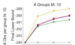
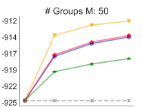
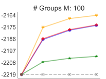
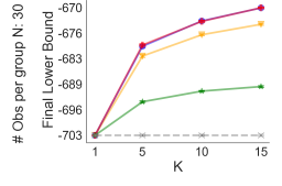
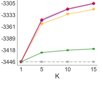
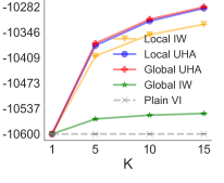
Figure 2: Inference results using locally-enhanced bounds and other baselines on synthetic datasets for varying number of groups (10, 50 and 100) and observations per group (10 and 30). The plots show the final lower bound achieved by different methods after training for 50k steps. All methods (local IW, local UHA, global IW, and global UHA) converge to plain VI for $K=1$. The dimensionality of the local variables $z_{i}$ is taken to be $d_{z}=5$ for the datasets with $N=10$ observations per group, and $d_{z}=20$ for the datasets with $N=30$ observations.

4 Related Work

There is a lot of work on related topics, such as the development of more flexible variational approximations (Tabak & Turner, 2013; Rezende & Mohamed, 2015), better tightening methods (Salimans et al., 2015; Domke & Sheldon, 2019), and more efficient variational methods for hierarchical models (Agrawal & Domke, 2021). Most of these represent contributions orthogonal to ours, and can be used jointly with our locally-enhanced bounds.

Normalizing flows (Tabak & Turner, 2013; Rezende & Mohamed, 2015; Kingma et al., 2016; Tomczak & Welling, 2016), for instance, are a powerful method to build flexible variational approximations using invertible parametric transformations. Since they typically require a large number of parameters, they are sometimes impractical for very high dimensional problems, such as those that arise when working with hierarchical models with many latent variables. Despite this, they can be used jointly with our method. One could use flows for each local approximation $q(z_{i}|\theta)$ and/or for the global approximation $q(\theta)$, and then optimize their parameters by maximizing a locally-enhanced bound.

Additionally, many powerful tightening methods have been developed (Agakov & Barber, 2004; Burda et al., 2016; Salimans et al., 2015; Domke & Sheldon, 2019; Geffner & Domke, 2021b; Zhang et al., 2021). All of these can be easily used to build locally-enhanced bounds following our construction from Section 3.3.

Specifically for hierarchical models, Hoffman & Blei (2015) introduced a flexible framework for fast stochastic variational inference. Their approach, however, requires conjugacy, limiting its applicability. To overcome this limitation, Agrawal & Domke (2021) proposed a parameter efficient algorithm that uses a single amortization network (Kingma & Welling, 2013) to parameterize all local approximations $q(z_{i}|\theta)$. This approach is compatible with our method, as this amortized variational distribution can be used with locally-enhanced bounds.

More generally, Ambrogioni et al. (2021) suggested the use of a variational approximation following the prior model’s structure. For the hierarchical models considered in this work, this results in a variational approximation with the same structure as the one shown in Equation 6, which was used by Hoffman & Blei (2015); Agrawal & Domke (2021), and is the one used in this work.

Finally, concurrently with this work, Jankowiak & Phan (2021) proposed several promising extensions for uncorrected Hamiltonian Annealing (Geffner & Domke, 2021b; Zhang et al., 2021). One of them involves its use for hierarchical models, applying it independently for each set of local variables. This is equivalent to a locally-enhanced bound built using uncorrected Hamiltonian Annealing. Although this is a minor focus of their work, it can be seen as an instance of our general framework.

5 Experiments

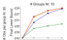
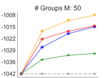
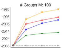
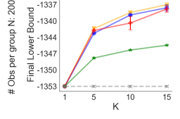
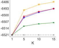
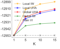
Figure 3: Inference results using locally-enhanced bounds and other baselines on MovieLens datasets of different sizes. The plots show the final lower bound achieved by different methods after training for 50k steps. All methods converge to plain VI for $K=1$.

This section presents an empirical evaluation of our new bounding technique. We perform variational inference using locally-enhanced bounds on multiple hierarchical models with real and synthetic datasets. We use a variational distribution $q(\theta,z)=q(\theta)\prod_{i=1}^{M}q(z_{i})$, where the approximation for the global variables $q(\theta)$ is set to be a factorized Gaussian, and the local approximations $q(z_{i})$ are taken to be independent of $\theta$ and also set to factorized Gaussians We test locally-enhanced bounds obtained using importance weighting and uncorrected Hamiltonian annealing for $K\in\{5,10,15\}$. We compare against plain VI, which trains the parameters of $q(\theta,z)$ by maximizing the $\mathcal{L}_{\mathrm{VI}}$ objective from Equation 7 (this corresponds to the “branch” approach from Agrawal & Domke (2021)), and against a direct/global application of importance weighting (objective from Equation 8) and uncorrected Hamiltonian annealing. (For the latter two baselines, the tightening methods are applied to all variables, local and global, jointly. See Figure 1.)

We optimize using Adam (Kingma & Ba, 2014) with a step-size $\eta=0.001$. For the plain VI baseline and the locally-enhanced bounds we use subsampling with $M^{\prime}=10$ to estimate gradients at each step using the reparameterization trick (Kingma & Welling, 2013; Titsias & Lázaro-Gredilla, 2014; Rezende et al., 2014). We do not use subsampling with the global application of importance weighting and uncorrected Hamiltonian annealing, as the methods do not support it. We initialize all methods to maximizers of the ELBO, and train for 50k steps. All results are reported together with their standard deviation, obtained using five different random seeds.

We clarify that the global importance weighting and global uncorrected Hamiltonian annealing baselines are also trained for 50k steps, using a full-batch approach to compute gradients at each iteration. This results in an optimization process that is significantly more expensive than that of other methods (locally-enhanced bounds and plain VI) which support subsampling.

5.1 Synthetic data

Model

We consider the hierarchical model given by

$$p(\mu_{z},\psi_{z},\psi_{y},z,y)=\mathcal{N}(\mu_{z}|0,1)\mathcal{N}(\psi_{z}|0,1)\\ \mathcal{N}(\psi_{y}|0,1)\prod_{i=1}^{M}\mathcal{N}(z_{i}|\mu_{z},e^{\psi_{z}})\prod_{j=1}^{N_{i}}\mathcal{N}(y_{ij}|z_{i}\,x_{ij},e^{\psi_{i}}),$$ (14)

where $x_{ij}$ is external information available for observation $y_{ij}$. In this case $\theta=(\mu_{z},\psi_{z},\psi_{y})$ represents the global variables and $z$ the local ones. While the above model defines the local variables $z_{i}$ to be one dimensional, they can also be defined to have an arbitrary dimension $d_{z}>1$, by setting $\mathcal{N}(z_{i}|\mathbf{1}_{d_{z}}\mu_{z},I_{d_{z}}e^{\psi_{z}})$ and $\mathcal{N}(y_{ij}|z_{i}^{\top}x_{ij},e^{\psi_{i}})$.

Datasets

We generated several datasets by sampling from the hierarchical model above. We consider different number of groups $M\in\{10,50,100\}$, and observations per group $N\in\{10,30\}$. In all cases, we sample components of $x_{ij}\in\mathbb{R}^{d_{z}}$ independently from a standard Gaussian.

Results

Results for all the generated datasets are shown in Figure 2. It can be observed that the use of locally-enhanced bounds yields significant improvements over plain VI, with the performance gap increasing for the larger values of $K$. It can also be observed that the use of locally-enhanced bounds leads to better results than the ones obtained using the global importance weighting baseline. While this baseline is somewhat competitive for the smaller models (left plots in Figure 2), it is severely outperformed by the use of locally-enhanced bounds in the larger models (right plots in Figure 2). This is despite the fact that the baseline is significantly more expensive to run, as it does not allow subsampling. On the other hand, we observe that the global uncorrected Hamiltonian baseline performs similarly to the locally-enhanced bound obtained using uncorrected Hamiltonian annealing. However, as mentioned above, this baseline is incompatible with subsampling, thus leading to a significantly more expensive optimization process.

Figure 5 in Appendix D shows the test log-likelihood achieved by each method for this model. It can be observed that methods based on uncorrected Hamiltonian annealing achieve the best log-likelihoods (both the global baseline and the locally-enhanced bound), followed by the locally-enhanced bound with importance weighting, and finally by a global application of importance weighting, which performs similarly to plain VI.

All results in Figure 2 were obtained for datasets which have the same number of observations for all local groups. To verify the effect that changing this may have, we ran additional simulations using a dataset which contained different number of observations for different groups. Specifically, we considered a dataset composed of $M=100$ groups, out of which 50 have only 2 observations, 30 have 5 observations, and 20 have 30 observations. Results are shown in Figure 4. Similar conclusions hold.

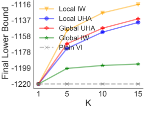
Figure 4: Inference results using locally-enhanced bounds and other baselines on a synthetic dataset generated with $M=100$ groups and a different number of observations per group (see main text). The plot shows the final lower bound achieved by different methods after training for 50k steps. All methods converge to the baseline plain VI for $K=1$.

5.2 Real data: Movie Lens

We now show results obtained using data from MovieLens100K (Harper & Konstan, 2015). This database contains 100k ratings from several users on $1700$ movies, where each movie comes with a feature vector $x\in\{0,1\}^{18}$ containing information about its genre. While the original ratings consist of discrete values between $1$ and $5$, we binarize them, assigning $0$ as “dislike” to ratings $(1,2,3)$, and $1$ as “like” to ratings $(4,5)$.

Model

We consider the hierarchical model given by

$$p(\mu_{z},\psi_{z},z,y)=\mathcal{N}(\mu_{z}|0,I)\mathcal{N}(\psi_{z}|0,I)\\ \prod_{i=1}^{M}\mathcal{N}(z_{i}|\mu_{z},e^{\psi_{z}})\prod_{j=1}^{N}\mathcal{B}(y_{ij}|z_{i}^{\top}x_{ij}),$$ (15)

where $x_{ij}\in\{0,1\}^{18}$ represents the feature vector for the $j$-th movie ranked by the $i$-th user, $\mu_{z}\in\mathbb{R}^{18}$ and $\psi_{z}\in\mathbb{R}^{18}$ represent the global variables $\theta$, and $z_{i}\in\mathbb{R}^{18}$ represents the local variables for group $i$, in this case the $i$-th user.

Datasets

We used data from MovieLens100K to generate several datasets with a varying number of users and ratings per user. Specifically, we consider three different number of users $M\in\{10,50,100\}$ and two different number of ratings per user $N\in\{30,200\}$.

Results

Results are shown in Figure 3. It can be observed that the locally-enhanced bound with importance weighting leads to the best results, followed by the locally-enhanced bound with uncorrected Hamiltonian annealing and the global application of uncorrected Hamiltonian annealing (which perform similarly). Finally, similarly to the results observed for the synthetic dataset, a global application of importance weighting and plain VI perform significantly worse.

6 Discussion and Future Work

We introduced locally-enhanced bounds, a new type of variational objective obtained by applying tightening methods at a local level for hierarchical models following Equation 1. The approach combines the efficiency of plain variational inference and the power of tightening methods while avoiding their drawbacks. An interesting direction for future work involves extending locally-enhanced bounds to more general models that do not follow a two level tree structure. We believe that developing methods able to automatically exploit conditional independences in arbitrary models to build locally-enhanced bounds would be extremely useful in practice.

Appendix A Proof of Theorem 3.2

Proof.

We have

$$\log p(y) =\operatornamewithlimits{\mathbb{E}}_{q(\theta)}\log\left(\frac{p(\theta)}{q(\theta)}p(y|\theta)\frac{q(\theta)}{p(\theta|y)}\right)$$

$$=\operatornamewithlimits{\mathbb{E}}_{q(\theta)}\left[\log\frac{p(\theta)}{q(\theta)}+\log p(y|\theta)+\log\frac{q(\theta)}{p(\theta|y)}\right]$$

$$=\operatornamewithlimits{\mathbb{E}}_{q(\theta)}\left[\log\frac{p(\theta)}{q(\theta)}+\sum_{i=1}^{M}\log p(y_{i}|\theta)\right]+\mathrm{KL}(q(\theta)\|p(\theta|y))$$

$$=\operatornamewithlimits{\mathbb{E}}_{q(\theta)}\left[\log\frac{p(\theta)}{q(\theta)}+\sum_{i=1}^{M}\mathcal{L}(q(z_{i}|\theta)\|p(z_{i},y_{i}|\theta))\right]$$

$$\quad+\sum_{i=1}^{M}\operatornamewithlimits{\mathbb{E}}_{q(\theta)}\left[\log p(y_{i}|\theta)-\mathcal{L}(q(z_{i}|\theta)\|p(z_{i},y_{i}|\theta))\right]+\mathrm{KL}(q(\theta)\|p(\theta|y)).$$

In the final equality, note that all terms on the second line are non-negative: the KL-divergence by definition and $\log p(y_{i}|\theta)-\mathcal{L}(q(z_{i}|\theta)\|p(z_{i},y_{i}|\theta))$ by assumption. ∎

Appendix B Details for AIS and UHA

This section introduces the details for AIS and UHA. We begin with a detailed description AIS, explain how it can be used with HMC transition kernels, and finally move on to UHA, which is built on those ideas.

Annealed Importance Sampling (AIS)

AIS can be seen as an instance of the auxiliary VI framework (Agakov & Barber, 2004). Given an initial approximation $q(z)$ and an unnormalized target distribution $p(z)$, AIS proceeds in four steps.

1. It builds a sequence of unnormalized densities $\pi^{1}(z),\ldots,\pi^{K-1}(z)$ that gradually bridge from $q(z)$ to the target $p(z)$.

2. It defines the forward transitions $T^{k}(z^{k+1}|z^{k})$ as an MCMC kernel that leaves the bridging density $\pi^{k}$ invariant, and the backward transitions $U^{k}(z^{k}|z^{k+1})$ as the reversal of $T^{k}$ with respect to $\pi^{k}$.

3. It uses the transition $T^{k}$ and $U^{k}$ to augment the variational and target density. This yields the augmented distributions

   $$q(z^{1:K}) =q(z^{1})\prod_{k=1}^{K-1}T^{k}(z^{k+1}|z^{k})$$ (16)

   $$p(z^{1:K}) =p(z^{K})\prod_{k=1}^{K-1}U^{k}(z^{k}|z^{k+1}).$$ (17)

4. It uses the augmented distributions to build the augmented ELBO, a lower bound on the log-normalizing constant of $p(z)$ as

   $$\operatornamewithlimits{\mathbb{E}}_{q(z^{1:K})}\log\frac{p(z^{K})}{q(z^{1})}\prod_{k=1}^{K-1}\frac{U^{k}(z^{k}|z^{k+1})}{T^{k}(z^{k+1}|z^{k})}.$$ (18)

   Then, using that $T^{k}(z^{k+1}|z^{k})\pi^{k}(z^{k})=U^{k}(z^{k}|z^{k+1})\pi^{k}(z^{k+1})$, the ratio from Equation 18 simplifies to

   $$\operatornamewithlimits{\mathbb{E}}_{q(z^{1:K})}\log\frac{p(z^{K})}{q(z^{1})}\prod_{k=1}^{K-1}\frac{\pi^{k}(z^{k})}{\pi^{k+1}(z^{k+1})}.$$ (19)

   This is the AIS lower bound. Its tightness depends on the specific Markov kernels used, with more powerful kernels leading to tighter bounds.

A particular Markov kernel that is known to work well is given by Hamiltonian Monte Carlo (HMC) (Neal et al., 2011; Betancourt, 2017). Integrating HMC with AIS is straightforward. It requires extending the initial distribution $q(z)$, the unnormalized target $p(z)$, and the bridging densities $\pi^{k}(z)$ with a momentum variable $\rho\sim r(\rho)$. Then, the transitions $T^{k}(z^{k+1},\rho^{k+1}|z^{k},\rho^{k})$ and $U^{k}(z^{k},\rho^{k}|z^{k+1},\rho^{k+1})$ as an HMC kernel and its reversal, respectively.

It has been observed that Hamiltonian AIS may yield tight lower bounds on the log marginal likelihood (Sohl-Dickstein & Culpepper, 2012; Grosse et al., 2015; Wu et al., 2017). Its main drawback, however, is that, due the use of a correction step in the HMC kernel, the resulting lower bound from Equation 19 is not differentiable, making tuning the method’s parameters hard. As we explain next, Uncorrected Hamiltonian Annealing addresses this drawback, building a fully-differentiable lower bound using an AIS-like procedure.

Uncorrected Hamiltonian Annealing (UHA)

UHA can be seen as a differentiable alternative to Hamiltonian AIS. It closely follows its derivation. It extends the variational distribution and target with the momentum variables $\rho\sim r(\rho)$, augments them using transitions $T^{k}(z^{k+1},\rho^{k+1}|z^{k},\rho^{k})$ and $U^{k}(z^{k},\rho^{k}|z^{k+1},\rho^{k+1})$, and builds the ELBO using these augmented distributions as

$$\operatornamewithlimits{\mathbb{E}}_{q(z^{1:K},\rho^{1:K})}\log\frac{p(z^{K})r(\rho^{K})}{q(z^{1})r(\rho^{1})}\prod_{k=1}^{K-1}\frac{U^{k}(z^{k},\rho^{k}|z^{k+1},\rho^{k+1})}{T^{k}(z^{k+1},\rho^{k+1}|z^{k},\rho^{k})}.$$ (20)

The main difference with Hamiltonian AIS comes in the choice for the transition. UHA sets $T^{k}$ to be an uncorrected HMC kernel targeting the bridging density $\pi^{k}(z,\rho)$. This transition consists of two steps, (partially) re-sampling the momentum from a distribution $s(\cdot|\rho^{k})$ that leaves $r(\rho)$ invariant, followed by the simulation of Hamiltonian dynamics without a correction step. Formally, this can be expressed as

$$\left.\begin{array}[]{l}T^{k}(z^{k+1},\rho^{k+1}|z^{k},\rho^{k}):\vspace{0.1cm}\\ \hskip 17.07182pt1.\quad\tilde{\rho}^{k}\sim s(\cdot|\rho^{k})\vspace{0.1cm}\\ \hskip 17.07182pt2.\quad(z^{k+1},\rho^{k+1})=\mathrm{Dynamics}(z^{k},\tilde{\rho}^{k}).\end{array}\right.$$ (21)

Similarly, UHA defines the backward transition $U^{k}$ as the uncorrected reversal of an HMC kernel that leaves $\pi^{k}(z,\rho)$ invariant (see Geffner & Domke (2021b) for details).

While closely related to Hamiltonian AIS, the use of uncorrected transition means that $U^{k}$ is no longer the reversal of $T^{k}$. Therefore, the simplification for the ratio $U^{k}/T^{k}$ used by AIS to go from Equation 18 to Equation 19 cannot be used. However, Geffner & Domke (2021b) and Zhang et al. (2021) showed that the ratio between these uncorrected transitions yields a simple expression,

$$\frac{U^{k}(z^{k},\rho^{k}|z^{k+1},\rho^{k+1})}{T^{k}(z^{k+1},\rho^{k+1}|z^{k},\rho^{k})}=\frac{r(\rho^{k})}{r(\tilde{\rho}^{k})},$$ (22)

where $\tilde{\rho}^{k}$ is defined in Equation 21. Then, the bound from Equation 20 can be expressed as (Geffner & Domke, 2021b; Zhang et al., 2021)

$$\operatornamewithlimits{\mathbb{E}}_{q(z^{1:K},\rho^{1:K})}\log\frac{p(z^{K})}{q(z^{1})}\prod_{k=1}^{K-1}\frac{r(\rho^{k+1})}{r(\tilde{\rho}^{k})},$$ (23)

which can be easily estimated using samples from the augmented proposal $q(z^{1:K},\rho^{1:K})$. UHA’s main benefit is that, in contrast to Hamiltonian AIS, it yields differentiable lower bounds that admit reparameterization gradients. This simplifies tuning all of the method’s parameters, which has been observed to yield large gains in practice (Geffner & Domke, 2021b; Zhang et al., 2021).

Appendix C Locally-enhanced bounds as divergence minimization

Tightening methods can be seen as minimizing a divergence in an augmented space (Domke & Sheldon, 2019). That is, a divergence between an augmented target and variational approximation. This section presents the locally-enhanced bounds obtained with UHA and IW from the perspective of minimizing a divergence in an augmented space, justifying the use of these methods for posterior approximation. Simply put, these constructions follow those by Domke & Sheldon (2018) and Geffner & Domke (2021b), but applied at the the local variables’ level. These constructions were provided by Sam Power.

C.1 Locally-enhanced bound with UHA

This section gives details on the construction of the augmented target and variational approximation that yield the locally-enhanced bound obtained with UHA. This uses a sequence of $K$ densities $\pi_{i}^{1}(z),\ldots,\pi_{i}^{K}(z)$ bridging between $q(z|\theta)$ and $p(z|\theta,y_{i})$ for each $i=1,\ldots,M$, and follows the construction from Appendix B but at the local variables’ level.

Augmented target

Given the target

$$p(\theta,z_{1:M}|y)=p(\theta|y)\prod_{i=1}^{M}p(z_{i}|\theta,y_{i}),$$ (24)

we apply the UHA augmentation (see Appendix B) for each local term $p(z_{i}|\theta,y_{i})$. That is, we define the $i$-th augmented local term using variables $z_{i}^{1:K}$ and $\rho_{i}^{1:K}$ as

$$p(z_{i}^{1:K},\rho_{i}^{1:K}|\theta,y_{i})=p(z_{i}^{K}|\theta,y_{i})r(\rho^{K})\prod_{k=1}^{K-1}U^{k}_{i}(z_{i}^{k},\rho_{i}^{k}|z_{i}^{k+1},\rho_{i}^{k+1},\theta,y_{i}),$$ (25)

where the transition $U^{k}_{i}$ corresponds to the uncorrected reversal of the HMC kernel targeting the $k$-th “local” bridging density $\pi_{i}^{k}$. Then, the final augmented target is given by

$$p(\theta,z_{1:M}^{1:K},\rho_{1:M}^{1:K}|y)=p(\theta|y)\prod_{i=1}^{M}p(z_{i}^{1:K},\rho_{i}^{1:K}|\theta,y_{i}).$$ (26)

Note that the marginal over $(\theta,z_{i:M}^{K})$ recovers the original target distribution from Equation 24.

Augmented variational approximation

We define the augmented $i$-th local approximation over variables $z_{i}^{1:K}$ and $\rho_{i}^{1:K}$ as

$$q(z_{i}^{1:K},\rho_{i}^{1:K}|\theta,y_{i})=q(z_{i}^{1}|\theta,y_{i})r(\rho_{i}^{1})\prod_{k=1}^{K-1}T^{k}_{i}(z_{i}^{k+1},\rho_{i}^{k+1}|z_{i}^{k},\rho_{i}^{k},\theta,y_{i}),$$ (27)

where $T_{i}^{k}$ is an uncorrected (underdamped) HMC kernel targeting the $k$-th “local” bridging density $\pi_{i}^{k}(z,\rho|\theta,y_{i})=\pi_{i}^{k}(z|\theta,y_{i})r(\rho)$. Then, the final variational approximation is given by

$$q(\theta,z_{1:M}^{1:K},\rho_{1:M}^{1:K}|y)=q(\theta|y)\prod_{i=1}^{M}q(z_{i}^{1:K},\rho_{i}^{1:K}|\theta,y_{i}).$$ (28)

Then, the marginal over $(\theta,z_{1:M}^{K})$ is used as an approximation of the original (un-augmented) target.

Recovering the locally-enhanced bound

Using the augmented distributions defined above we get the following decomposition of the marginal likelihood

$$\log p(y)=\mathcal{L}_{\mathrm{VI}}\left(q(\theta,z_{1:M}^{1:K},\rho_{1:M}^{1:K}|y)\|p(\theta,z_{1:M}^{1:K},\rho_{1:M}^{1:K}|y)\right)+\mathrm{KL}\left(q(\theta,z_{1:M}^{1:K},\rho_{1:M}^{1:K}|y)\|p(\theta,z_{1:M}^{1:K},\rho_{1:M}^{1:K}|y)\right),$$ (29)

where the first term in the RHS is exactly the locally-enhanced bound obtained with UHA. Since $\log p(y)$ is constant, maximizing the locally-enhanced bound is equivalent to minimizing the KL-divergence between the augmented distributions. Finally, the chain-rule of the KL-divergence (Cover, 1999) justifies the use of the marginal $q(\theta,z_{1:M}^{K}|y)$ as the approximation to the original target distribution.

C.2 Locally-enhanced bound with IW

The derivation follows that of Domke & Sheldon (2018), but applied at the local level (as done above for UHA). We refer the reader to the work by Domke & Sheldon (2018) for details regarding the construction.

Appendix D Test log-likelihoods for synthetic model

Figure 5 presents log-likelihoods obtained by each method on a held-out test set.

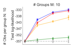
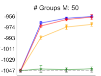
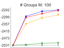
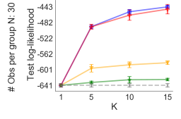
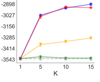
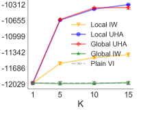
Figure 5: Test log-likelihoods achieved by each method on synthetic datasets of different sizes. The plots show the test log-likelihoods achieved by different methods after training for 50k steps. All methods converge to plain VI for $K=1$. The dimensionality of the local variables $z_{i}$ is taken to be $d_{z}=5$ for the datasets with $N=10$ observations per group, and $d_{z}=20$ for the datasets with $N=30$ observations.

References

- Agakov & Barber (2004) Agakov, F. V. and Barber, D. An auxiliary variational method. In International Conference on Neural Information Processing, pp. 561–566. Springer, 2004.
- Agrawal & Domke (2021) Agrawal, A. and Domke, J. Amortized variational inference for simple hierarchical models. Advances in Neural Information Processing Systems, 34, 2021.
- Ajalloeian & Stich (2020) Ajalloeian, A. and Stich, S. U. On the convergence of sgd with biased gradients. arXiv preprint arXiv:2008.00051, 2020.
- Ambrogioni et al. (2021) Ambrogioni, L., Lin, K., Fertig, E., Vikram, S., Hinne, M., Moore, D., and van Gerven, M. Automatic structured variational inference. In International Conference on Artificial Intelligence and Statistics, pp. 676–684. PMLR, 2021.
- Bardenet et al. (2017) Bardenet, R., Doucet, A., and Holmes, C. On markov chain monte carlo methods for tall data. The Journal of Machine Learning Research, 18(1):1515–1557, 2017.
- Bengtsson et al. (2008) Bengtsson, T., Bickel, P., and Li, B. Curse-of-dimensionality revisited: Collapse of the particle filter in very large scale systems. In Probability and statistics: Essays in honor of David A. Freedman, pp. 316–334. Institute of Mathematical Statistics, 2008.
- Betancourt (2015) Betancourt, M. The fundamental incompatibility of hamiltonian monte carlo and data subsampling. arXiv preprint arXiv:1502.01510, 2015.
- Betancourt (2017) Betancourt, M. A conceptual introduction to hamiltonian monte carlo. arXiv preprint arXiv:1701.02434, 2017.
- Blei et al. (2003) Blei, D. M., Ng, A. Y., and Jordan, M. I. Latent dirichlet allocation. Journal of machine Learning research, 3(Jan):993–1022, 2003.
- Blei et al. (2017) Blei, D. M., Kucukelbir, A., and McAuliffe, J. D. Variational inference: A review for statisticians. Journal of the American Statistical Association, 112(518):859–877, 2017.
- Burda et al. (2016) Burda, Y., Grosse, R., and Salakhutdinov, R. Importance weighted autoencoders. In Proceedings of the International Conference on Learning Representations, 2016.
- Challis & Barber (2013) Challis, E. and Barber, D. Gaussian kullback-leibler approximate inference. Journal of Machine Learning Research, 14(8), 2013.
- Chatterjee & Diaconis (2018) Chatterjee, S. and Diaconis, P. The sample size required in importance sampling. The Annals of Applied Probability, 28(2):1099–1135, 2018.
- Cover (1999) Cover, T. M. Elements of information theory. John Wiley & Sons, 1999.
- Cremer et al. (2017) Cremer, C., Morris, Q., and Duvenaud, D. Reinterpreting importance-weighted autoencoders. arXiv preprint arXiv:1704.02916, 2017.
- Cressie et al. (2009) Cressie, N., Calder, C. A., Clark, J. S., Hoef, J. M. V., and Wikle, C. K. Accounting for uncertainty in ecological analysis: the strengths and limitations of hierarchical statistical modeling. Ecological Applications, 19(3):553–570, 2009.
- Domke & Sheldon (2018) Domke, J. and Sheldon, D. Importance weighting and variational inference. In Advances in Neural Information Processing Systems, 2018.
- Domke & Sheldon (2019) Domke, J. and Sheldon, D. Divide and couple: Using monte carlo variational objectives for posterior approximation. In Advances in Neural Information Processing Systems, 2019.
- Geffner & Domke (2021a) Geffner, T. and Domke, J. Empirical evaluation of biased methods for alpha divergence minimization. In Symposium on Advances in Approximate Bayesian Inference, 2021a.
- Geffner & Domke (2021b) Geffner, T. and Domke, J. Mcmc variational inference via uncorrected hamiltonian annealing. Advances in Neural Information Processing Systems, 34, 2021b.
- Gelman (2006) Gelman, A. Multilevel (hierarchical) modeling: what it can and cannot do. Technometrics, 48(3):432–435, 2006.
- Gelman & Hill (2006) Gelman, A. and Hill, J. Data analysis using regression and multilevel/hierarchical models. Cambridge university press, 2006.
- Grosse et al. (2015) Grosse, R. B., Ghahramani, Z., and Adams, R. P. Sandwiching the marginal likelihood using bidirectional monte carlo. arXiv preprint arXiv:1511.02543, 2015.
- Harper & Konstan (2015) Harper, F. M. and Konstan, J. A. The movielens datasets: History and context. Acm transactions on interactive intelligent systems (tiis), 5(4):1–19, 2015.
- Hoffman & Blei (2015) Hoffman, M. and Blei, D. Stochastic structured variational inference. In Artificial Intelligence and Statistics, pp. 361–369. PMLR, 2015.
- Hoffman et al. (2013) Hoffman, M. D., Blei, D. M., Wang, C., and Paisley, J. Stochastic variational inference. The Journal of Machine Learning Research, 14(1):1303–1347, 2013.
- Jankowiak & Phan (2021) Jankowiak, M. and Phan, D. Surrogate likelihoods for variational annealed importance sampling. arXiv preprint arXiv:2112.12194, 2021.
- Jordan et al. (1999) Jordan, M. I., Ghahramani, Z., Jaakkola, T. S., and Saul, L. K. An introduction to variational methods for graphical models. Machine learning, 37(2):183–233, 1999.
- Kingma & Ba (2014) Kingma, D. P. and Ba, J. Adam: A method for stochastic optimization. arXiv preprint arXiv:1412.6980, 2014.
- Kingma & Welling (2013) Kingma, D. P. and Welling, M. Auto-encoding variational bayes. In Proceedings of the International Conference on Learning Representations, 2013.
- Kingma et al. (2016) Kingma, D. P., Salimans, T., Jozefowicz, R., Chen, X., Sutskever, I., and Welling, M. Improved variational inference with inverse autoregressive flow. Advances in neural information processing systems, 29:4743–4751, 2016.
- Kreft & De Leeuw (1998) Kreft, I. G. and De Leeuw, J. Introducing multilevel modeling. Sage, 1998.
- Lax & Phillips (2012) Lax, J. R. and Phillips, J. H. The democratic deficit in the states. American Journal of Political Science, 56(1):148–166, 2012.
- Lim & Teh (2007) Lim, Y. J. and Teh, Y. W. Variational bayesian approach to movie rating prediction. In Proceedings of KDD cup and workshop, volume 7, pp. 15–21. Citeseer, 2007.
- Maddison et al. (2017) Maddison, C. J., Lawson, D., Tucker, G., Heess, N., Norouzi, M., Mnih, A., Doucet, A., and Teh, Y. W. Filtering variational objectives. arXiv preprint arXiv:1705.09279, 2017.
- Naesseth et al. (2020) Naesseth, C. A., Lindsten, F., and Blei, D. Markovian score climbing: Variational inference with kl (p—— q). arXiv preprint arXiv:2003.10374, 2020.
- Neal (2001) Neal, R. M. Annealed importance sampling. Statistics and computing, 11(2):125–139, 2001.
- Neal et al. (2011) Neal, R. M. et al. Mcmc using hamiltonian dynamics. Handbook of markov chain monte carlo, 2(11):2, 2011.
- Rezende & Mohamed (2015) Rezende, D. J. and Mohamed, S. Variational inference with normalizing flows. In Proceedings of the 32nd International Conference on Machine Learning (ICML-15), 2015.
- Rezende et al. (2014) Rezende, D. J., Mohamed, S., and Wierstra, D. Stochastic backpropagation and approximate inference in deep generative models. In Proceedings of the 31st International Conference on Machine Learning (ICML-14), pp. 1278–1286, 2014.
- Royle & Dorazio (2008) Royle, J. A. and Dorazio, R. M. Hierarchical modeling and inference in ecology: the analysis of data from populations, metapopulations and communities. Elsevier, 2008.
- Salimans et al. (2015) Salimans, T., Kingma, D., and Welling, M. Markov chain monte carlo and variational inference: Bridging the gap. In International Conference on Machine Learning, pp. 1218–1226, 2015.
- Snijders & Bosker (2011) Snijders, T. A. and Bosker, R. J. Multilevel analysis: An introduction to basic and advanced multilevel modeling. sage, 2011.
- Sohl-Dickstein & Culpepper (2012) Sohl-Dickstein, J. and Culpepper, B. J. Hamiltonian annealed importance sampling for partition function estimation. arXiv preprint arXiv:1205.1925, 2012.
- Tabak & Turner (2013) Tabak, E. G. and Turner, C. V. A family of nonparametric density estimation algorithms. Communications on Pure and Applied Mathematics, 66(2):145–164, 2013.
- Thin et al. (2021) Thin, A., Kotelevskii, N., Doucet, A., Durmus, A., Moulines, E., and Panov, M. Monte carlo variational auto-encoders. In International Conference on Machine Learning, pp. 10247–10257. PMLR, 2021.
- Titsias & Lázaro-Gredilla (2014) Titsias, M. and Lázaro-Gredilla, M. Doubly stochastic variational bayes for non-conjugate inference. In Proceedings of the 31st International Conference on Machine Learning (ICML-14), pp. 1971–1979, 2014.
- Tomczak & Welling (2016) Tomczak, J. M. and Welling, M. Improving variational auto-encoders using householder flow. arXiv preprint arXiv:1611.09630, 2016.
- Vallerand (1997) Vallerand, R. J. Toward a hierarchical model of intrinsic and extrinsic motivation. Advances in experimental social psychology, 29:271–360, 1997.
- Wainwright et al. (2008) Wainwright, M. J., Jordan, M. I., et al. Graphical models, exponential families, and variational inference. Foundations and Trends® in Machine Learning, 1(1–2):1–305, 2008.
- Wolf et al. (2016) Wolf, C., Karl, M., and van der Smagt, P. Variational inference with hamiltonian monte carlo. arXiv preprint arXiv:1609.08203, 2016.
- Wu et al. (2017) Wu, Y., Burda, Y., Salakhutdinov, R., and Grosse, R. On the quantitative analysis of decoder-based generative models. In Proceedings of the International Conference on Learning Representations, 2017.
- Zhang et al. (2021) Zhang, G., Hsu, K., Li, J., Finn, C., and Grosse, R. B. Differentiable annealed importance sampling and the perils of gradient noise. Advances in Neural Information Processing Systems, 34, 2021.