Sensitivity analysis under the $f$-sensitivity models:
a distributional robustness perspective

Abstract

This paper introduces the $f$-sensitivity model, a new sensitivity model that characterizes the violation of unconfoundedness in causal inference. It assumes the selection bias due to unmeasured confounding is bounded “on average”; compared with the widely used point-wise sensitivity models in the literature, it is able to capture the strength of unmeasured confounding by not only its magnitude but also the chance of encountering such a magnitude.

We propose a framework for sensitivity analysis under our new model based on a distributional robustness perspective. We first show that the bounds on counterfactual means under the $f$-sensitivity model are optimal solutions to a new class of distributionally robust optimization (DRO) programs, whose dual forms are essentially risk minimization problems. We then construct point estimators for these bounds by applying a novel debiasing technique to the output of the corresponding empirical risk minimization (ERM) problems. Our estimators are shown to converge to valid bounds on counterfactual means if any nuisance component can be estimated consistently, and to the exact bounds when the ERM step is additionally consistent. We further establish asymptotic normality and Wald-type inference for these estimators under slower-than-root-$n$ convergence rates of the estimated nuisance components. Finally, the performance of our method is demonstrated with numerical experiments.

1 Introduction

In a variety of areas, conducting randomized trial can be costly, unethical or even infeasible. To draw causal conclusions, researchers/policy-makers need to resort to observational data. The particular challenge in observational studies is confounding: because the treatment allocation mechanism is completely unknown, there might exist variables that affect both the treatment and the outcomes. With unmeasured confounding, causal conclusions drawn from naïvely comparing the outcomes for the treated and untreated units – even after adjusting for the difference in the observable characteristics – can be invalid.

An example is the well-known debate over the effect of smoking (the treatment) on the development of lung cancer (the outcome), where one observes a higher prevalence of lung cancer among smokers and concludes that smoking causes lung cancer. The criticism of Fisher, (1958) argues that this effect may instead be entirely driven by genetics: even for two people with the same observed characteristics (e.g., demographic information and medical history), the one who is genetically more likely to develop lung cancer may also be genetically more likely to smoke; should this be true, even though smoking may not cause the lung cancer, we could still observe a higher proportion of lung cancer among the treated group even after matching the observed characteristics. In this case, the genetic factor could be an unmeasured confounder that induces the nontrivial observed effect and potentially leads to a faulty causal conclusion.

To formalize the discussion, we follow the potential outcome framework (Neyman,, 1923; Imbens and Rubin,, 2015) and posit a data-generating distribution $\mathbb{P}$ on $(X,U,T,Y(1),Y(0))$, where $X\in\mathcal{X}$ is the observed covariate vector in a compact set $\mathcal{X}\subset\mathbb{R}^{p}$, $U\in\mathcal{U}$ is the unobserved confounding factor, $T\in\{0,1\}$ is the treatment option ($T=1$ for receiving the treatment and $T=0$ for control), and $Y(1)\in\mathbb{R}$ and $Y(0)\in\mathbb{R}$ are the two potential outcomes. We assume access to a dataset $\{(X_{i},T_{i},Y_{i})\}_{i=1}^{n}$ of $n$ i.i.d. triplets generated from $\mathbb{P}$, where for unit $i$, $Y_{i}=Y_{i}(T_{i})$ is the observed outcome under treatment $T_{i}$, Without loss of generality (since $U$ is arbitrary), under $\mathbb{P}$, one has

$$\big{(}Y(1),Y(0)\big{)}\leavevmode\nobreak\ \rotatebox[origin={c}]{90.0}{$\models$}\leavevmode\nobreak\ T{\,|\,}X,U.$$ (1)

We are interested in the average treatment effect (ATE): $\mathbb{E}[Y(1)-Y(0)]$, the average treatment effect on the control (ATC): $\mathbb{E}[Y(1)-Y(0){\,|\,}T=0]$, and the average treatment effect on the treated (ATT): $\mathbb{E}[Y(1)-Y(0){\,|\,}T=1]$, where in all quantities the expectation is taken with respect to the underlying joint distribution. To make progress, we assume that there is sufficient exploration in the dataset, known as the overlap assumption in the literature. We define the observed propensity score $e(x):=\mathbb{P}(T=1{\,|\,}X=x)$.

Assumption 1 (Overlap).

$0<e(x)<1$ for $\mathbb{P}$-almost all $x\in\mathcal{X}$.

Under the overlap assumption, the identification and estimation of treatment effects in observational studies have mostly relied on the unconfoundedness condition (a.k.a. strong ignorability (Rosenbaum and Rubin, 1983b, )): $\big{(}Y(1),Y(0)\big{)}\leavevmode\nobreak\ \rotatebox[origin={c}]{90.0}{$\models$}\leavevmode\nobreak\ T{\,|\,}X$. That is, all confounders that could simultaneously affect the treatment assignment and the outcomes have been measured in $X$. In the lung cancer example, this condition imposes that for all people with the same value of $X$, even though their genetics and potential outcomes differ, they are equally likely to become a smoker (receive the treatment).

The strong ignorability condition, however, is not testable and is often hard to justify in practice. Sensitivity analysis offers a way to bypass this obstacle. In the lung cancer example, Cornfield et al., (1959) for the first time used the method of sensitivity analysis: it strongly supports the existence of treatment effects by showing that a genetic factor must be nine times more prevalent in smokers than in non-smokers in order to explain the observed effect should there be no actual treatment effects (and it is high implausible to find such a genetic factor). At a high level, sensitivity analysis starts with a sensitivity model on how the unknown data generating process deviates from the strong ignorability condition, and then estimates the range – rather than a single value – of the treatment effects, thus offering a quantitative understanding of how robust the causal conclusion is against potential unmeasured confounding. The method in Cornfield et al., (1959) was generalized by Rosenbaum’s $\Gamma$-selection condition (Rosenbaum,, 1987), a pioneering model on the selection bias that has become a classic. Tan, (2006) later proposed the marginal sensitivity model, based on which a series of work have developed various treatment effects estimation and inference schemes  (Zhao et al.,, 2017; Kallus et al.,, 2019; Lee et al.,, 2020; Dorn and Guo,, 2021; Jin et al.,, 2021; Nie et al.,, 2021; Dorn et al.,, 2021). The marginal sensitivity model centers around the key quantity

$${\textnormal{OR}}(x,u)=\frac{\mathbb{P}(T=1{\,|\,}X=x)/\mathbb{P}(T=0{\,|\,}X=x)}{\mathbb{P}(T=1{\,|\,}X=x,U=u)/\mathbb{P}(T=0{\,|\,}X=x,U=u)},$$ (2)

the odds ratio of receiving treatment conditional only on observed covariates versus conditional on both unmeasured confounders and observed covariates. Intuitively, ${\textnormal{OR}}(x,u)$ quantifies the impact of unmeasured confounding on the treatment probability. Tan, (2006) assumes uniformly bounded odds ratio:

$$\frac{1}{\Gamma}\leq{\textnormal{OR}}(x,u)\leq\Gamma$$ (3)

for $\mathbb{P}$-almost all $x\in{\mathcal{X}}$ and $u\in{\mathcal{U}}$ for some $\Gamma\geq 1$. When $\Gamma=1$, this assumption recovers the unconfoundedness assumption, and the larger the $\Gamma$, the more confoundness the model tolerates.

Despite being widely used, the marginal $\Gamma$-selection model (3) can be limited in some cases. We illustrate this point with a simple and natural parametric example, which also motivates our new sensitivity model.

Example 1.

Let us consider a simple example without covariates. We assume the observed probability of treatment is $\mathbb{P}(T=1)=1/2$. In this context, the strong ignorability condition means all units receive treatments with the same probability. The researcher would like to estimate the range of $\mathbb{E}[Y(1){\,|\,}T=0]$ if the observational data is confounded to some extent. Based on some background knowledge, she is in particular worried about a confounder $U\sim\mathcal{N}(0,1)$, where $T{\,|\,}U\sim\textsf{Bern}\big{(}\frac{\exp(\delta U)}{1+\exp(\delta U)}\big{)}$ for some $\delta\in(0,1)$. By construction, the odds ratio characterizing the selection bias caused by $U$ is

$${\textnormal{OR}}(U):=\frac{\mathbb{P}(T=0{\,|\,}U)}{\mathbb{P}(T=1{\,|\,}U)}\cdot\frac{\mathbb{P}(T=1)}{\mathbb{P}(T=0)}=e^{-\delta U}.$$ (4)

Since $U$ is unbounded, the above odds ratio cannot be uniformly bounded by any constant. In this simple stylized example, this researcher cannot obtain any informative range of the treatment effects from the sensitivity analysis under a hypothesized marginal $\Gamma$-selection assumption (3). $\square$

More generally, if a researcher concerns a scenario where the unmeasured confounding is drastically severe in a small region of the sample space but non-exists in the remaining, it would require a very large, if not infinity, value of $\Gamma$ for (3) to be practically meaningful. Sensitivity analysis under (3) thus provides a wide (thus uninformative) range of treatment effects. However, since the magnitude of selection bias is large only in a small region, its overall impact (on ATE for instance) should still be small. A desirable sensitivity model should still produce informative bounds on the treatment effects in such situations, and more generally, capture the strength of unmeasured confounding beyond its maximum magnitude.

We do mention that a few works in the literature (Imbens,, 2003; Franks et al.,, 2019) postulate parametric models for treatment assignment that is affected by unobserved confounders; such parametric models include the simple example discussed here as a special case and hence allow for unbounded local confounded effects. However, the key limitation is that the proposed confounding model is highly specialized to the logistic form, whereas the marginal $\Gamma$-selection criterion provides a non-parametric model that is quite general.

Motivated by the merits of both worlds, in this paper, we develop a novel sensitivity model that describes the “average” strength of unmeasured confounding. We also develop a framework to conduct sensitivity analysis with our new models, which informs the range of treatment effects under various overall strength of unmeasured confounding. Our contributions are summarized in the following.

• A new sensitivity model. We propose the $f$-sensitivity model, a general, non-parametric model that characterizes the overall strength of unmeasured confounding. It is suitable for situations where the confounding may be unbounded yet with a limited overall impact at the population level.

• A new class of distributional robustness problems. We show that the partial identification bounds on treatment effects under the $f$-sensitivity model can be represented by the solution to a class of DRO programs that are new to the literature, providing a distributional robustness perspective to sensitivity analysis under unmeasured confounding.

• A new framework for robust estimation and inference. We develop a set of tools to estimate the optimal objective of the new DRO problems; the objective can be expressed via the solution to a weighted risk minimization problem, with the unknown weights determined by the covariate shift between treatment and control groups. We then propose estimators for the bounds using a new debiasing technique applied to the output of the corresponding ERM problem. We prove that our estimators are doubly-robust to the estimation of nuisance components. Furthermore, they enjoy an interesting one-sided validity property that is specific to the partial identification setting: our estimators are still valid yet perhaps conservative bounds when the ERM step is completely off.

2 The new $f$-sensitivity model

2.1 The $(f,\rho)$-selection condition

Our new $f$-sensitivity model is specified by the following $(f,\rho)$-selection condition.

Definition 1 (The $(f,\rho)$-selection condition).

Suppose $f:\mathbb{R}_{+}\mapsto\mathbb{R}$ is a convex function such that $f(1)=0$. Let ${\textnormal{OR}}(x,u)$ be defined in (2). $\mathbb{P}$ satisfies the $(f,\rho)$-selection condition if for $\mathbb{P}$-almost all $x$,

$$d_{f}(\mathbb{P}):=\max\bigg{\{} \int f\big{(}{\textnormal{OR}}(x,U)\big{)}\textnormal{d}\mathbb{P}_{U\mid X=x,T=1},\leavevmode\nobreak\ \int f\big{(}{\textnormal{OR}}(x,U)^{-1}\big{)}\big{)}\textnormal{d}\mathbb{P}_{U{\,|\,}X=x,T=0}\bigg{\}}\leq\rho.$$ (5)

This new model addresses the unbounded confounding issue in Example 1: even though the odds ratio is not uniformly bounded, it is controlled overall; in this case, our new model can be a more reasonable description of the practical situation. We will discuss shortly about more settings where our method may be sensible. Now, let us first address the concern in Example 1 using our framework.

Example 1 (Continued).

We take $f(t)=t\log t$, a convex function with $f(1)=0$. Continuing the computation in Example 4, the first term of $d_{f}(\mathbb{P})$ in Definition 1 can be computed as

$$\int f\big{(}{\textnormal{OR}}(U)\big{)}{\,\mathrm{d}}\mathbb{P}_{U{\,|\,}T=1}=\int-\delta U\cdot e^{-\delta U}{\,\mathrm{d}}\mathbb{P}_{U{\,|\,}T=1}=-\delta\int u\cdot e^{-\delta u}\cdot\frac{2e^{\delta u}}{1+e^{\delta u}}\cdot\frac{1}{\sqrt{2\pi}}e^{-u^{2}/2}{\,\mathrm{d}}u<\infty.$$ (6)

The right-handed side is approximately $0.2$ if we take $\delta=1$ and $0.6$ if we take $\delta=2$. Note that $\int f\big{(}{\textnormal{OR}}(U)\big{)}{\,\mathrm{d}}\mathbb{P}_{U{\,|\,}T=1}$ can be interpreted as the overall deviation of ${\textnormal{OR}}(U)$ from $1$ in the treated (observed) group, which is bounded, even though ${\textnormal{OR}}(U)\rightarrow\infty$ when $U\rightarrow-\infty$. In this way, one could seamlessly use our framework to conduct sensitivity analysis; this will inform the impact of the overall strength of unmeasured confounding on the treatment effects. $\square$

Two remarks on the $(f,\rho)$-selection condition are in order.

Remark 1.

If $\mathbb{P}$ satisfies the marginal $\Gamma$-selection condition (3), then it automatically satisfies the $(f,\rho)$-selection condition with any qualified $f$ and $\rho=\max\{f(1/\Gamma),f(\Gamma)\}$. This can easily be checked by noting that (3) implies $f({\textnormal{OR}}(x,U))\leq\max\{f(1/\Gamma),f(\Gamma)\}$ by convexity of $f$, and similarly by the symmetry of (3) $f({\textnormal{OR}}(x,U)^{-1})\leq\max\{f(1/\Gamma),f(\Gamma)\}$, thereby leading to the bound on $d_{f}(\mathbb{P})$. It might appear that the $(f,\rho)$-selection condition is weaker than the marginal $\Gamma$-selection condition. However, we do note the two models give different characterizations, as for a distribution that satisfies marginal $\Gamma$-selection condition, it might satisfy $(f,\rho)$-selection condition for some $\rho$ that is much smaller than $\max\{f(1/\Gamma),f(\Gamma)\}$.

Remark 2.

In the definition of $d_{f}(\mathbb{P})$, we take the maximum of two integrals, each from one direction. This is mainly to keep the condition symmetric with regards to the choice of the treated or control groups, and align with the convention in the sensitivity models in the literature (Tan,, 2006). That said, as we would see shortly in Section 2.3, it might be more natural to only work with one of them (i.e. assume one of them be bounded by $\rho$) when one of the counterfactuals is of primal interest.

2.2 Comparison with other sensitivity models

To better interpret the $(f,\rho)$-selection condition and illustrate its difference from the (marginal) $\Gamma$-selection condition (3), we provide a unified perspective on the sensitivity models. We first note a crucial property of ${\textnormal{OR}}(X,U)$, a key quantity that characterizes the impact of unmeasured confounding.

Property 1.

Let ${\textnormal{OR}}(x,u)$ be defined in (2). Then $\mathbb{E}\big{[}{\textnormal{OR}}(X,U){\,|\,}X,T=1\big{]}=1$ almost surely, where the conditional distribution is induced by the joint distribution of $(X,U,T)$. Also, ${\textnormal{OR}}(X,U)=1$ holds $\mathbb{P}_{X,U{\,|\,}T=1}$-almost surely under the strong ignorability condition $T\,\rotatebox[origin={c}]{90.0}{$\models$}\,(Y(1),Y(0)){\,|\,}X$.

At a high level, both the $(f,\rho)$-selection and the marginal $\Gamma$-selection condition quantify how faraway the nonnegative mean-one random variable ${\textnormal{OR}}(x,U)$ is from the constant one. The marginal $\Gamma$-selection condition (3) requires the maximum fluctuation of ${\textnormal{OR}}(x,U)$ to be bounded within $[1/\Gamma,\Gamma]$ all the time. The $(f,\rho)$-selection condition, on the other hand, characterizes the overall distance of ${\textnormal{OR}}(x,U)$ from a constant. When we take $f(x)=\frac{1}{2}|x-1|$, the $(f,\rho)$-selection condition is similar to bounds on the total variation (TV) distance; when $f(x)=(x-1)^{2}$, the $(f,\rho)$-selection condition resembles bounds on the $\chi^{2}$-distance between ${\textnormal{OR}}(x,U)$ and one. Different choices of $f$ pose different penalty for large values of confounding. For example, taking $f(x)=\frac{1}{2}|x-1|$, the contribution to the confounding measure is proportional to the absolute distance from $1$. For $f(x)=(x-1)^{2}$, the contribution to the confounding strength is larger for larger scale of confounding.

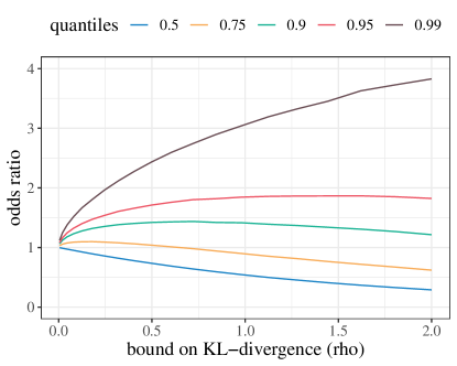
We now illustrate the distinction between the $(f,\rho)$-selection condition and the marginal $\Gamma$-selection condition in two cases. First, in the left panel of Figure 1 we see three possible ${\textnormal{OR}}(x,U)$ as functions of $U$, all of which integrate to $1$ and with $U\sim\textrm{Unif}[0,1]$. There, the solid line is a constant function and indicates no unmeasured confounding. Among the other two, intuitively, the dotted curve has “smaller” confounding because most of the time the odds ratio is quite close to $1$; one could imagine that in these regions, erroneously making the strong ignorability assumption may not incur too much bias. However, the upper bound on ${\textnormal{OR}}(x,U)$ is large due to a small proportion of severe confounding at the left. In this case, although we imagine that the impact of $U$ for the dotted and dashed curves are drastically different, it requires the same $\Gamma$ in (3) to characterize them. As a result, partial identification bounds for treatment effects under the marginal $\Gamma$-selection condition may be uninformative; a better measure for the confounding strength may instead be the overall fluctuation of ${\textnormal{OR}}(x,U)$ around $1$.

Figure 1: Left: examples of ${\textnormal{OR}}(x,U)$ that are quite different but have similar upper bounds. Right: examples of ${\textnormal{OR}}(x,U)$ that are similar but have drastically different upper bounds.

The right panel of Figure 1 plots another scenario where the uniform bound can be inaccurate. Here, the dotted and dashed lines describe two confounded cases where ${\textnormal{OR}}(x,U)$ almost coincide except for the tail at the left end. The dotted thus requires a much larger $\Gamma$ than the dashed one in the marginal sensitivity model, if not infinity. In this case, because the treatment probabilities (decided by the odds ratio) in these cases are so close and the tail region only takes a tiny part of the population, one could imagine the impact of confounding on the treatment effect to be close. Hence, besides the scale of confounding, a sensitivity model should also takes into account the change of having certain confounding strength.

Our $(f,\rho)$-selection condition exactly aims at resolving the above issues. For general choice of $f$, our sensitivity measure would give starkly different measures for the two cases in the left panel of Figure 1, while providing similar measures for those in the right panel. This is because it is an “average” measure of the deviation of ${\textnormal{OR}}(x,U)$ from the constant one for strong ignorability. Correspondingly, sensitivity analysis from our model informs what would happen under a specific level of overall confounding strength.

2.3 Distributional shifts under the $f$-sensitivity model

The first observation in this paper relates the observables to the counterfactuals. We characterize the distributional shifts between the two under our $f$-sensitivity model, which identifies a new class of robust inference problems that, as far as we know, are new to the literature.

We cast causal inference as a counterfactual inference problem: one needs to impute the missing outcome, i.e., the counterfactual, to estimate treatment effects at the population level. For example, to estimate the ATC: $\mathbb{E}[Y(1){\,|\,}T=0]-\mathbb{E}[Y(0){\,|\,}T=0]$, one needs to impute the first term, the counterfactual mean of $Y(1)$ in the control group. The distribution of the unobservable $(X,Y(1))$ in the control group is

$$\mathbb{P}_{X,Y(1){\,|\,}T=0}=\underbrace{\mathbb{P}_{X{\,|\,}T=0}}_{\rm(a)}\times\underbrace{\mathbb{P}_{Y(1){\,|\,}X,T=0}}_{\rm(b)}.$$

Here part (a) is identifiable from the observations, but part (b) is not when there is unmeasured confounding. Our first result states that under the $(f,\rho)$-selection condition, (b) is bounded from its counterpart in the observable in terms of $f$-divergence.

Definition 2 ($f$-divergence).

Let $\mathbb{P}$ and $\mathbb{Q}$ be two probability distributions over a space $\Omega$ such that $\mathbb{P}$ is absolutely continuous with respect to $\mathbb{Q}$. For a convex function $f$ such that $f(1)=0$, the $f$-divergence of $\mathbb{P}$ from $\mathbb{Q}$ is defined as $D_{f}(\mathbb{P}\,\|\,\mathbb{Q})=\mathbb{E}_{\mathbb{Q}}\big{[}f(\frac{{\,\mathrm{d}}\mathbb{P}}{{\,\mathrm{d}}\mathbb{Q}})\big{]}$, where $\frac{{\,\mathrm{d}}\mathbb{P}}{{\,\mathrm{d}}\mathbb{Q}}$ is the Radon-Nikodym derivative.

Popular examples for $f$-divergence in the literature include the Kullback–Leibler (KL) divergence with $f(t)=t\log t$, the total variation (TV) distance with $f(t)=|t-1|/2$, Pearson $\chi^{2}$-divergence with $f(t)=(t-1)^{2}$, and the Cressie-Read family of $f$-divergences (Cressie and Read,, 1984) parametrized by $k$, where $f_{k}(t):=\frac{t^{k}-kt+k-1}{k(k-1)}$. Throughout this paper, we work with generic forms of $f$-divergence, and provide discussions on concrete examples where proper conditions are satisfied for our analysis.

Lemma 1.

Under the $(f,\rho)$-selection condition, we have

$$D_{f}\big{(}\mathbb{P}_{Y(1){\,|\,}X=x,T=0}\,\|\,\mathbb{P}_{Y(1){\,|\,}X=x,T=1}\big{)}\leq\rho$$

for $\mathbb{P}_{X{\,|\,}T=1}$-almost all $x$; that is, the $f$-divergence between the conditional distributions in the two groups are bounded by $\rho$ for almost all $X$ in group $T=1$.

Proof of Lemma 1.

Suppose a distribution $\mathbb{P}$ over $(X,U,T,Y(0),Y(1))$ satisfies the $(f,\rho)$-selection condition. By condition (1) and the data-processing inequality,

$$D_{f}\big{(}\mathbb{P}_{Y(1){\,|\,}X=x,T=0}\leavevmode\nobreak\ \|\leavevmode\nobreak\ \mathbb{P}_{Y(1){\,|\,}X=x,T=1}\big{)}\leq D_{f}\big{(}\mathbb{P}_{Y(1),U{\,|\,}X=x,T=0}\leavevmode\nobreak\ \|\leavevmode\nobreak\ \mathbb{P}_{Y(1),U{\,|\,}X=x,T=1}\big{)}$$

$$= \mathbb{E}_{Y(1),U{\,|\,}X=x,T=1}\bigg{[}f\Big{(}\frac{{\,\mathrm{d}}\mathbb{P}_{Y(1),U{\,|\,}X=x,T=0}}{{\,\mathrm{d}}\mathbb{P}_{Y(1),U{\,|\,}X=x,T=1}}\Big{)}\bigg{]}.$$

We note that the likelihood ratio can be decomposed as

$$\frac{{\,\mathrm{d}}\mathbb{P}_{Y(1),U{\,|\,}X=x,T=0}}{{\,\mathrm{d}}\mathbb{P}_{Y(1),U{\,|\,}X=x,T=1}} =\frac{{\,\mathrm{d}}\mathbb{P}_{Y(1){\,|\,}U,X=x,T=0}}{{\,\mathrm{d}}\mathbb{P}_{Y(1){\,|\,}U,X=x,T=1}}\cdot\frac{{\,\mathrm{d}}\mathbb{P}_{U{\,|\,}X=x,T=0}}{{\,\mathrm{d}}\mathbb{P}_{U{\,|\,}X=x,T=1}}$$

$$\stackrel{{\scriptstyle\rm(a)}}{{=}}\frac{{\,\mathrm{d}}\mathbb{P}_{U{\,|\,}X=x,T=0}}{{\,\mathrm{d}}\mathbb{P}_{U{\,|\,}X=x,T=1}}=\frac{\mathbb{P}(T=0{\,|\,}X=x,U)}{\mathbb{P}(T=1{\,|\,}X=x,U)}\cdot\frac{\mathbb{P}(T=1{\,|\,}X=x)}{\mathbb{P}(T=0{\,|\,}X=x)},$$

where step (a) is due to condition (1). Combining the above two facts yields

$$D_{f}\big{(}\mathbb{P}_{Y(1){\,|\,}X,T=0}\leavevmode\nobreak\ \|\leavevmode\nobreak\ \mathbb{P}_{Y(1){\,|\,}X,T=1}\big{)}\leq \mathbb{E}_{Y(1),U{\,|\,}X,T=1}\bigg{[}f\Big{(}\frac{\mathbb{P}(T=0{\,|\,}X,U)}{\mathbb{P}(T=1{\,|\,}X,U)}\cdot\frac{\mathbb{P}(T=1{\,|\,}X)}{\mathbb{P}(T=0{\,|\,}X)}\Big{)}\bigg{]}$$

$$= \mathbb{E}_{U{\,|\,}X,T=1}\bigg{[}f\Big{(}\frac{\mathbb{P}(T=0{\,|\,}X,U)}{\mathbb{P}(T=1{\,|\,}X,U)}\cdot\frac{\mathbb{P}(T=1{\,|\,}X)}{\mathbb{P}(T=0{\,|\,}X)}\Big{)}\bigg{]}\leq\rho$$

almost surely, where the last inequality is due to the $(f,\rho)$-selection condition. ∎

We complete our characterization of the counterfactual distributions $\mathbb{P}_{X,Y(1){\,|\,}T=0}$ induced by all super-populations that agrees with the observables and satisfies our sensitivity models.

Proposition 1.

Let $\mathbb{P}^{\sup}$ be the true unknown super-population over $(X,U,T,Y(0),Y(1))$ and let $\mathcal{P}$ be the set of all distributions over $(X,U,T,Y(0),Y(1))$. Let $\mathbb{P}^{\textnormal{obs}}_{X,Y,T}$ be the joint distribution of all observable random variables $(X,Y,T)$. Define $\mathcal{Q}_{1,0}$ to be the ambiguity set of all counterfactual distributions that agrees with the observables and satisfies the $(f,\rho)$ selection condition, i.e.,

$$\mathcal{Q}_{1,0}=\big{\{}\mathbb{P}_{X,Y(1){\,|\,}T=0}\colon\mathbb{P}\in\mathcal{P},\leavevmode\nobreak\ \mathbb{P}_{X,Y,T}=\mathbb{P}^{\textnormal{obs}}_{X,Y,T},\leavevmode\nobreak\ \mathbb{P}\,\text{satisfies Definition\leavevmode\nobreak\ \ref{def:cond}}\,\big{\}}.$$

Then $\mathbb{P}^{\sup}_{X,Y(1){\,|\,}T=0}\in\mathcal{Q}_{1,0}$, and

$$\mathcal{Q}_{1,0}\subset\Big{\{}\mathbb{Q}\colon{\textstyle\frac{{\,\mathrm{d}}\mathbb{Q}_{X}}{{\,\mathrm{d}}\mathbb{P}_{X{\,|\,}T=1}^{\textnormal{obs}}}}(x)=r_{1,0}(x),\leavevmode\nobreak\ D_{f}\big{(}\mathbb{Q}_{Y{\,|\,}X=x}\leavevmode\nobreak\ \big{\|}\leavevmode\nobreak\ \mathbb{P}_{Y{\,|\,}X=x,T=1}^{\textnormal{obs}}\big{)}\leq\rho,\leavevmode\nobreak\ \text{for }\mathbb{P}^{\textnormal{obs}}_{X{\,|\,}T=t}\text{-almost all }x\Big{\}},$$ (7)

where $r_{1,0}(x)=\frac{(1-e(x))p_{1}}{e(x)(1-p_{1})}$, and $e(x)=\mathbb{P}^{\textnormal{obs}}(T=1{\,|\,}X=x)$, $p_{1}=\mathbb{P}^{\textnormal{obs}}(T=1)$.

We defer the proof of Proposition 1 to Appendix A, where we prove a stronger version that gives a tight characterization of $\mathcal{Q}_{1,0}$. Symmetrically, we can also define $\mathcal{Q}_{0,1}$ as the identification set of $\mathbb{P}_{X,Y(0){\,|\,}T=1}$; the tight characterization of $\mathcal{Q}_{0,1}$ is also given in Appendix A. From now on, we only consider the ambiguity sets in Proposition 1 to emphasize the more general distributional robustness aspect of this problem.

Proposition 1 identifies a new class of robust inference problems, where the target distribution has an identifiable $X$-shift and the unidentifiable conditional distribution is restricted in $f$-divergence ball; it is similar to the ambiguity set studied in Jin et al., (2021). This model is closely related to, but quite distinct from other ambiguity sets involving $f$-divergence in the literature (Duchi and Namkoong,, 2021; Si et al.,, 2020; Andrews et al.,, 2020) that only concern marginal (joint) distributions.

Remark 3 (Relation to other $f$-divergence bounds).

Previous works in the literature (see Section 2.4 for a summary) often work under the $f$-divergence ball around the marginal distribution $\mathbb{P}_{X,Y}$, characterized by

$$\widetilde{\mathcal{Q}}=\big{\{}\mathbb{Q}\colon D_{f}\big{(}\mathbb{Q}_{X,Y}\big{\|}\mathbb{P}_{X,Y}\big{)}\ \leq\rho\big{\}}.$$ (8)

While in our formulation, the ambiguity sets take the form

$$\begin{array}[]{l}\mathcal{Q}=\Big{\{}\mathbb{Q}\colon\frac{{\,\mathrm{d}}\mathbb{Q}_{X}}{{\,\mathrm{d}}\mathbb{P}_{X}}(x)=r(x),\leavevmode\nobreak\ D_{f}\big{(}\mathbb{Q}_{Y{\,|\,}X}\big{\|}\mathbb{P}_{Y{\,|\,}X}\big{)}\ \leq\rho\Big{\}},\end{array}$$ (10)

where $r(x)$ is a known or identifiable function. Such distinction is similar to what has been observed in Jin et al., (2021, Remark 3). Instead of bounding the overall shift as in (8), the constraint in (10) actually allows freedom in the shift of $X$: the sets in (10) can be small as long as $\rho$ is small. For counterfactual inference under the strong ignorability condition, the set (10) can be a singleton even if $\mathbb{P}_{X}$ and $\widetilde{\mathbb{P}}_{X}$ are drastically different, while (8) might require a large $\rho$ to hold. More generally, when there is a known (or estimable) large shift in $\mathbb{P}_{X}$ but a relatively small shift in $\mathbb{P}_{Y{\,|\,}X}$, (10) provides a tighter range of the target distributions, and the methods we develop in this paper can be directly applied.

2.4 Related work

This work falls within a strand of sensitivity analysis that models the impact of unmeasured confounding through bounds on selection bias. We summarize a few of them that are not mentioned above. Remarkably, Rosenbaum and Rubin, 1983a studies the impact of selection bias among matched pairs, which is further extended by a series of works (Rosenbaum,, 1987; Gastwirth et al.,, 1998; Rosenbaum, 2002b, ; Rosenbaum, 2002a, ) to sensitivity models that uniformly bounds the selection bias among samples with matching covariates. Also related to sensitivity analysis under uniformly bounded selection bias is Yadlowsky et al., (2018), which works under an extention of Rosenbaum’s sensitivity model that is similar to Tan, (2006). Besides modelling the selection bias among treatment, observed covariates and unmeasured confounders, we mention in passing that Ding and VanderWeele, (2016) considers the sensitivity analysis of other metrics than treatment effects.

We develop our framework based on observing the distributional shift between the observations and the counterfactuals. This perspective echos the ideas of several previous works (Jin et al.,, 2021; Yadlowsky et al.,, 2018; Dorn et al.,, 2021) on sensitivity analysis. In particular, we formulate the estimand via an optimization problem under constraints on distributional shifts, similar to Yadlowsky et al., (2018); Dorn et al., (2021). However, as we work under different sensitivity models, both the form of distributional shifts and the techniques for statistical estimation and inference are distinct.

$f$-divergence is often used to characterize discrepancy between distributions (Rényi,, 1961; Morimoto,, 1963; Csiszár,, 1964; Liese and Vajda,, 2006; Rahman,, 2016). In our work, we use a quantity similar to $f$-divergence to measure the deviation of the odds ratio from $1$, hence characterizing the overall magnitude of the selection bias caused by unmeasured confounding. This in turn leads to the bounded $f$-divergence between the conditional distribution of the counterfactuals and that of the observations under our model, while the covariate distributional shift is identifiable from the data. To the best of our knowledge, this type of distributional shifts have not been studied before.

By connecting sensitivity analysis to distributionally robust optimization, this works is also related to a line of work on estimation, inference and learning under various types of distributional shifts, e.g., $f$-divergence, outside the task of inferring causal effects. Among them, Christensen and Connault, (2019) places bounds on the marginal distributions of hidden variables in structural equation models; Andrews et al., (2020) studies parameter estimation when the joint distributions of variables are within an $f$-divergence ball; Duchi and Namkoong, (2021) studies the empirical risk minimization problem when the joint distribution of $(X,Y)$ shifts within an $f$-divergence ball; Si et al., (2020) studies the policy learning for contextual bandits under unknown marginal distribution shifts; Gupta and Rothenhäusler, (2021) studies the estimation and inference of statistical parameters under distributional shifts in certain directions, etc. The new class of robust inference problems in our work is different from the settings of these works. We also develop a set of tools for estimation and inference under this new type of distributional shifts.

Finally, because the covariate shifts need to be estimated, we propose a debiasing technique to obtain root-$n$ rate of inference when the nuisance components are estimated with slower convergence rates. This is also generally connected to a vast body of missing data literature with unknown missing mechanisms, although in different contexts and with different details. In particular, we use the cross-fitting (Schick,, 1986; Zheng and Laan,, 2011; Chernozhukov et al.,, 2018) technique to mitigate the error in nuisance component estimation; bias correction using a different dataset under covariate shift is also related to and inspired by the transductive inference technique in Jin and Rothenhäusler, (2021).

3 Sensitivity analysis under the new model

3.1 Bounds on the treatment effects

In this part, we study the (population-level) partial identification bounds on counterfactual means under our sensitivity model. They are provided as solutions to convex optimization problems that only involve identifiable quantities. We consider $\mathbb{E}[Y(1){\,|\,}T=0]$ for illustration.

Proposition 2.

Let $\mu_{1,0}^{-}$ (resp. $\mu_{1,0}^{+})$ be the optimal objective function of the convex optimization problem

$$\mathop{\min(\text{resp.\leavevmode\nobreak\ }\max)}_{L(x,y)\textnormal{\leavevmode\nobreak\ measurable}}\leavevmode\nobreak\ \mathbb{E}\big{[}Y(1)L(X,Y(1))\,\big{|}\,T=1\big{]}$$ (11)

s.t. $$\mathbb{E}[L(x,Y(1)){\,|\,}X=x,T=1]=r_{1,0}(x)$$ (12)

$$\mathbb{E}\big{[}f\big{(}L(x,Y(1))/r_{1,0}(x)\big{)}\,\big{|}\,X=x,T=1\big{]}\leq\rho,\quad\mbox{for almost all }x,$$ (13)

where all the expectations are induced by the observed distribution. Then $\mu_{1,0}^{-}\leq\mathbb{E}[Y(1){\,|\,}T=0]\leq\mu_{1,0}^{+}$ under the $(f,\rho)$-selection condition.

As we have discussed, the counterfactual means are the building blocks for treatment effects. Proposition 2 immediately implies bounds on the ATC: denote the observable group-wise means as $\mu^{\textnormal{obs}}_{t}:=\mathbb{E}[Y(t){\,|\,}T=t]$ for $t\in\{0,1\}$, then under the $(f,\rho)$-selection condition, the ATC is bounded as

$$\mu_{1,0}^{-}-\mu^{\textnormal{obs}}_{0}\leq\mathbb{E}[Y(1)-Y(0){\,|\,}T=0]\leq\mu_{1,0}^{+}-\mu^{\textnormal{obs}}_{0}.$$ (14)

Switching the role of $1$ and $0$ in Proposition 2, one can obtain bounds on $\mathbb{E}[Y(0){\,|\,}T=1]$; let $\mu^{+}_{0,1}$ and $\mu^{-}_{0,1}$ denote the upper and lower bound on $\mathbb{E}[Y(0){\,|\,}T=1]$, respectively, we then get bounds on the ATT:

$$\mu^{\textnormal{obs}}_{1}-\mu_{0,1}^{+}\leq\mathbb{E}[Y(1)-Y(0){\,|\,}T=1]\leq\mu^{\textnormal{obs}}_{1}-\mu_{0,1}^{-}.$$

By the decomposition of ATE (average treatment effects), we also have the representation of lower and upper bounds for $\mathbb{E}[Y(1)-Y(0)]$. Under the $(f,\rho)$-selection condition, we have

$$p_{1}\big{(}\mu^{\textnormal{obs}}_{1}-\mu_{0,1}^{+}\big{)}+p_{0}\big{(}\mu_{1,0}^{-}-\mu^{\textnormal{obs}}_{0}\big{)}\leq\mathbb{E}[Y(1)-Y(0)]\leq p_{1}\big{(}\mu^{\textnormal{obs}}_{1}-\mu_{0,1}^{-}\big{)}+p_{0}\big{(}\mu_{1,0}^{+}-\mu^{\textnormal{obs}}_{0}\big{)}.$$ (15)

Estimation of these bounds thus boil down to that of $\mu_{t,1-t}^{\pm}$ under our sensitivity models, the optimal objective value of the convex optimization problems in Proposition 2.

Remark 4.

As we mentioned before, optimal objectives of the problems in Proposition 2 are not necessarily tight bounds for counterfactual means. To align with the literature and keep a relatively clean formulation of dual problems, we only account for the direction $D_{f}(\mathbb{P}_{Y(1){\,|\,}X=x,T=0}\leavevmode\nobreak\ \|\leavevmode\nobreak\ \mathbb{P}_{Y(1){\,|\,}X,T=1})\leq\rho$ when considering $\mathbb{E}[Y(1){\,|\,}T=0]$. For completeness, we discuss the tight bounds on counterfactual means, hence ATT and ATC, in Section 6. We also note that combining sharp bounds on ATT and ATC does not necessarily lead to sharp bounds on ATE, as they might be attained by different super-populations. We leave the investigation of sharp bounds on ATEs for future pursuit.

3.2 From the primal to the dual

It is hard to directly solve the infinite-dimensional optimization problem (11). We address this issue by translating to its dual form which might be easier to tackle. In the following, we primarily focus on $\mu_{1,0}^{-}$, the lower bound on $\mathbb{E}[Y(1){\,|\,}T=0]$, and the same idea carries over to the upper bounds as well as bounds for other quantities. Proposition 3 represents $\mu_{1,0}^{-}$ via a dual formulation, whose proof is in Appendix C.1.

Proposition 3.

The optimal objective of (11) is given by

$$\mu_{1,0}^{-} =-\inf_{\alpha(X)\geq 0,\eta(X)\in\mathbb{R}}\mathbb{E}\bigg{[}r_{1,0}(X)\Big{\{}\alpha(X)f^{*}\Big{(}\frac{Y(1)+\eta(X)}{-\alpha(X)}\Big{)}+\eta(X)+\alpha(X)\rho\Big{\}}\,\bigg{|}\,T=1\bigg{]},$$ (16)

where $f^{*}(s)=\sup_{t\geq 0}\{st-f(t)\}$ is the conjugate function of $f$. In particular, denoting $\ell(\alpha,\eta,x,y)=\alpha f^{*}(\frac{y+\eta}{-\alpha})+\eta+\alpha\rho$ for $(\alpha,\eta)\in\mathbb{R}^{+}\times\mathbb{R}$, we have $\mu_{1,0}^{-}=-\mathbb{E}\big{[}\ell(\alpha^{*}(X),\eta^{*}(X),X,Y(1))\,\big{|}\,T=1\big{]},$ where for $\mathbb{P}_{X{\,|\,}T=1}$-almost all $x$,

$$\big{(}\alpha^{*}(x),\eta^{*}(x)\big{)}\in\underset{\alpha\geq 0,\eta\in\mathbb{R}}{\arg\!\min}\leavevmode\nobreak\ \mathbb{E}\bigg{[}\alpha f^{*}\Big{(}\frac{Y(1)+\eta}{-\alpha}\Big{)}+\eta+\alpha\rho\,\bigg{|}\,X=x,T=1\bigg{]}.$$ (17)

Our task is then to estimate the dual formulation (16), which can be viewed as a risk minimization problem. However, in sharp contrast to ERM problems in the literature, it involves a typically unknown weight $r_{1,0}(x)$ which depends on the propensity score $e(x)=\mathbb{P}(T=1{\,|\,}X=x)$. As the estimation rate of this quantity is often slower than root-$n$, directly solving (16) with plug-in weights might yield inaccurate estimators and prohibit root-$n$ statistical inference.

To address this issue, we will make use of the second observation in Proposition 3: $(\alpha^{*}(x),\eta^{*}(x))$, the optimizer for (16), is also the minimizer of per-$x$ conditional risk. This property crucially allows us to estimate $\alpha^{*}(\cdot)$ and $\eta^{*}(\cdot)$ without knowledge of $r_{1,0}(\cdot)$. Our general idea is to employ empirical risk minimization tools to estimate $\alpha^{*}(\cdot),\eta^{*}(\cdot)$, and then estimate $\mu_{1,0}^{-}$ by plugging into (16). Still, the slow estimation rate for the weights and the optimizers poses additional challenges for statistical inference. We will also develop a novel adjustment technique to still achieve root-$n$ inference when these quantities are estimated at a slow rate.

Before introducing our procedures, we present a result on the behavior of the optimizer $\alpha^{*}(x)$: it is positive as long as $\mathbb{P}_{Y(1){\,|\,}X,T=1}$ does not have a large point mass at its essential infimum and the function $f$ satisfy some regularity conditions in the limit. The proof of Proposition 4 is deferred to Appendix B.1.

Proposition 4.

Define $\underline{y}(x)=\sup\big{\{}t:\mathbb{P}(Y(1)<t{\,|\,}X=x,T=1)=0\big{\}}$ and $\bar{p}(x)=\mathbb{P}\big{(}Y(1)=\underline{y}(x){\,|\,}X=x,T=1\big{)}$. We assume that $\bar{p}(x)f(1/\bar{p}(x))+(1-\bar{p}(x))f(0)>\rho$ for $\mathbb{P}_{X{\,|\,}T=1}$-almost all $x$. Also suppose there exist constants $L$ and $U$ such that $f(x)^{*}\geq L$ for $x\in\mathbb{R}$, $f^{*}(x)\leq U$ for $x\leq 0$, $\lim_{x\rightarrow-\infty}f^{*}(x)/x=0$ and $\lim_{x\rightarrow\infty}f^{*}(x)/x=\infty$. Then the solution to (16) satistifies $\alpha^{*}(x)>0$ for $\mathbb{P}_{X{\,|\,}T=1}$-almost all $x$.

In particular, the conditions on $f$ hold for a large variety of functions; concrete examples include KL divergence, where $f(x)=x\log x$ and $f^{*}(x)=e^{x-1}$, as well as $\chi^{2}$-divergence, where $f(x)=(x-1)^{2}$ and $f^{*}(x)=\frac{1}{4}((x+2)_{+}^{2}-1)$, etc.

In the following, we assume throughout that the conditions of Proposition 4 hold, hence by the compactness of $\mathcal{X}$, there exists some $\epsilon>0$ such that $\alpha^{*}(x)>\epsilon$ for $\mathbb{P}_{X{\,|\,}T=1}$-almost all $x$ . An important implication is that, as $\alpha^{*}(x)$ lies in the interior of $[0,\infty)$, the gradient of the risk function is typically mean-zero at $(\alpha^{*}(x),\eta^{*}(x))$; this would play an important role in achieving root-$n$ statistical inference.

3.3 The estimation procedure

We start with splitting samples in the treated and control groups into three equally sized folds, denoted as $\mathcal{I}_{1}^{(j)},\mathcal{I}_{0}^{(j)}$, $j=1,2,3$, respectively. For each $j=1,2,3$, we use samples in $\mathcal{I}^{(j+1)}_{1}$ and $\mathcal{I}_{0}^{(j+1)}$ to obtain an estimator $\widehat{r}^{(j)}$ for $r_{1,0}$, and solve an empirical risk minimization (ERM) problem to obtain estimators $\widehat{\alpha}^{(j)}$ and $\widehat{\eta}^{(j)}$ for $(\alpha^{*},\eta^{*})$ without knowledge of $r_{1,0}$; this empirical risk minimization step will be discussed shortly after. We then define the function

$$\widehat{H}^{(j)}(x,y)=\widehat{\alpha}^{(j)}(x)f^{*}\Big{(}\frac{y+\widehat{\eta}^{(j)}(x)}{-\widehat{\alpha}^{(j)}(x)}\Big{)}+\widehat{\eta}^{(j)}(x)+\widehat{\alpha}^{(j)}(x)\rho.$$

Using data in $\mathcal{I}_{1}^{(j+2)}$, we run a regression algorithm to obtain an estimator $\widehat{h}^{(j)}$ for $\bar{h}^{(j)}(x):=\mathbb{E}\big{[}\widehat{H}^{(j)}(X,Y(1))\,\big{|}\,X=x,T=1,\mathcal{I}_{1}^{(j+1)}\big{]},$ where we view $\widehat{\alpha}^{(j)}$ and $\widehat{\eta}^{(j)}$, hence $\widehat{H}^{(j)}$, as fixed functions (e.g., by conditioning on $\mathcal{I}_{1}^{(j+1)}$ and $\mathcal{I}_{0}^{(j)}$. Finally, we define the estimator

$$\widehat{\mu}_{1,0}^{(j)}=\frac{1}{|\mathcal{I}_{1}^{(j)}|}\sum_{i\in\mathcal{I}_{1}^{(j)}}\widehat{r}^{(j)}(X_{i})\big{(}\widehat{H}^{(j)}(X_{i},Y_{i})-\widehat{h}^{(j)}(X_{i})\big{)}+\frac{1}{|\mathcal{I}_{0}^{(j)}|}\sum_{i\in\mathcal{I}_{0}^{(j)}}\widehat{h}^{(j)}(X_{i}).$$

The above procedure is repeated for each $j=1,2,3$, and we average the three estimators to obtain

$$\widehat{\mu}_{1,0}^{-}=-\frac{1}{3}\sum_{j=1}^{3}\widehat{\mu}_{1,0}^{(j)}.$$

The whole procedure is summarized in Algorithm 1. In the algorithm, we refer to $\mathcal{I}^{(k)}_{1}$ for some $k>3$ as $\mathcal{I}^{(k\text{ mod }3)}_{1}$; the same principle applies to $\mathcal{I}_{0}^{(k)}$. We let $\mathcal{R}(\cdot,\cdot)$ to be a generic algorithm that uses data in $\mathcal{I}_{1}$ and $\mathcal{I}_{0}$ to obtain an estimator $\mathcal{R}(\mathcal{I}_{1},\mathcal{I}_{0})$ for $r$. We use $\textsf{ERM}(\cdot)$ to denote a generic ERM algorithm that uses any data $\mathcal{I}$ to output an estimator $\textsf{ERM}(\mathcal{I})$ for $(\alpha^{*}(\cdot),\eta^{*}(\cdot))$. We let Reg$(\cdot)$ denote a generic regression algorithm that takes data $(X_{i},Z_{i})_{i\in\mathcal{I}}$ to output an estimator Reg$(Z_{i}\sim X_{i},\leavevmode\nobreak\ i\in\mathcal{I})$ for $\mathbb{E}[Z{\,|\,}X=\cdot]$.

Algorithm 1 Estimation procedure for $\mu^{-}_{1,0}$

0:  Treated samples $\mathcal{I}_{1}$; control samples $\mathcal{I}_{0}$; the algorithm $\mathcal{R}$ for estimating $r$; the ERM algorithm $\textsf{ERM}(\cdot)$ for estimating $(\alpha,\eta)$; the regression algorithm Reg$(\cdot)$ for obtaining $\bar{h}$.

1:  Randomly split $\mathcal{I}_{1}$ and $\mathcal{I}_{0}$ into three equal-sized groups: $\mathcal{I}_{1}^{(j)},\mathcal{I}_{0}^{(j)}$, $j=1,2,3$.

2:  for $j=1,2,3$ do

3:     Estimate $r_{1,0}$: obtain $\widehat{r}^{(j)}(\cdot)\leftarrow\mathcal{R}\big{(}\mathcal{I}_{1}^{(j+1)},\mathcal{I}_{0}^{(j+1)}\big{)}$.

4:     Estimate $(\alpha^{*},\eta^{*})$: obtain $(\widehat{\alpha}^{(j)}(\cdot),\widehat{\eta}^{(j)}(\cdot))\leftarrow\textsf{ERM}\big{(}\mathcal{I}_{1}^{(j+1)}\big{)}$

5:     Conditional regression: $\widehat{h}^{(j)}(\cdot)\leftarrow\textsf{Reg}(\widehat{H}^{(j)}(X_{i},Y_{i})\sim X_{i},\leavevmode\nobreak\ i\in\mathcal{I}_{1}^{(j+2)})$.

6:     Compute $\widehat{\mu}_{1,0}^{(j)}\leftarrow\frac{1}{|\mathcal{I}_{1}^{(j)}|}\sum_{i\in\mathcal{I}_{1}^{(j)}}\widehat{r}^{(j)}(X_{i})\big{(}\widehat{H}^{(j)}(X_{i},Y_{i})-\widehat{h}^{(j)}(X_{i})\big{)}+\frac{1}{|\mathcal{I}_{0}^{(j)}|}\sum_{i\in\mathcal{I}_{0}^{(j)}}\widehat{h}^{(j)}(X_{i}).$

7:  end for

7:  Estimator $\widehat{\mu}^{-}_{1,0}=-\frac{1}{3}\sum_{j=1}^{3}\widehat{\mu}_{1,0}^{(j)}$.

In Algorithm 1, the subroutines $\mathcal{R}(\cdot,\cdot)$ and Reg$(\cdot)$ are standard: to estimate $r_{1,0}$, one could use $\mathcal{I}_{1}^{(j+1)}\cup\mathcal{I}_{0}^{(j+1)}$ to estimate the propensity score $e(x)$ with any regression algorithm, and then plug in the definition of $r_{1,0}$. Similarly, Reg$(\cdot)$ can be any regression algorithm that fits a conditional mean function given i.i.d. data. Widely adopted regression methods in the literature include localized nonparametric methods like kernel regression (Nadaraya,, 1964; Watson,, 1964), local polynomial regression (Cleveland,, 1979; Cleveland and Devlin,, 1988), smoothing spline (Green and Silverman,, 1993) and modern machine learning methods including regression trees (Breiman et al.,, 1984) and random forests (Ho,, 1995), to name a few. The ERM step is relatively unique to our problem, and we discuss it in more details with rigorous guarantees as follows.

3.4 Solving for $\widehat{\alpha}(\cdot)$ and $\widehat{\eta}(\cdot)$

We take a moment to elaborate on the estimation of $\widehat{\theta}^{(j)}:=(\widehat{\alpha}^{(j)},\widehat{\eta}^{(j)})$. From Proposition 3, $\theta^{*}:=(\alpha^{*},\eta^{*})$ is also the population risk minimizer of $\mathbb{E}[\ell(\theta,X,Y(1)){\,|\,}T=1]$ (i.e., removing $r_{1,0}(x)$), where the loss function

$$\ell(\theta,x,y)=\alpha(x)f^{*}\Big{(}\frac{y+\eta(x)}{-\alpha(x)}\Big{)}+\eta(x)+\alpha(x)\rho$$

is convex in $\theta=(\alpha,\eta)$. The empirical risk is correspondingly (recall that we run ERM with fold $\mathcal{I}_{1}^{(j+1)}$)

$$\widehat{\mathbb{E}}_{n}\big{[}\ell(\theta,X,Y(1))\big{]}=\frac{1}{|\mathcal{I}_{1}^{(j+1)}|}\sum_{i\in\mathcal{I}_{1}^{(j+1)}}\ell(\theta,X_{i},Y_{i}).$$

We can thus consider a function class $\Theta$, and solve for the empirical risk minimization (ERM) problem. This approach is similar to Yadlowsky et al., (2018); however, they express the bounds of conditional expectations of counterfactuals themselves as empirical risk minimizers, while we use this ERM step as an intermediate step and employ distinct downstream techniques. To solve this ERM problem, we use the method of sieves (Geman and Hwang,, 1982); we consider an increasing sequence $\Theta_{1}\subset\Theta_{2}\subset\cdots$ of spaces of smooth functions, and let

$$\widehat{\theta}^{(j)}=\underset{\theta\in\Theta_{n}}{\arg\!\min}\leavevmode\nobreak\ \widehat{\mathbb{E}}_{n}\big{[}\ell(\theta,X,Y(1))\big{]}.$$

We consider two examples of seives inspired by Yadlowsky et al., (2018).

Example 2 (Polynomials).

Let Pol$(J)$ be the space of $J$-th order polynomials on $[0,1]$:

$$\textrm{Pol}(J,\epsilon)=\Big{\{}x\mapsto{\textstyle\sum_{k=0}^{J}}a_{k}x^{k}\colon a_{k}\in\mathbb{R}\Big{\}},$$

and let Pol$(J,\epsilon)$ be the space of $J$-th order polynomials on $[0,1]$ truncated at $\epsilon>0$:

$$\textrm{Pol}(J,\epsilon)=\Big{\{}x\mapsto\max\{\epsilon,{\textstyle\sum_{k=0}^{J}}a_{k}x^{k}\big{\}}\colon a_{k}\in\mathbb{R}\Big{\}}.$$

Then we define the sieve $\Theta_{n}=\Theta_{n}^{\alpha}\times\Theta_{n}^{\eta}$, where $\Theta_{n}^{\alpha}=\{x\mapsto\prod_{k=1}^{d}f_{k}(x_{k})\colon f_{k}\in\mathrm{Pol}(J_{n},0),k=1,\dots,d\}$ and $\Theta_{n}^{\eta}=\{x\mapsto\prod_{k=1}^{d}f_{k}(x_{k})\colon f_{k}\in\mathrm{Pol}(J_{n}),k=1,\dots,d\}$ for $J_{n}\to\infty$.

Compared to Yadlowsky et al., (2018), our function class additionally truncates the functions away from zero for $\alpha(x)$: we note that, if $\alpha^{*}(x)$ is always positive (implied by the minimality of the risk function and Proposition 4) and continuous (satisfied if $\mathbb{P}_{Y(1){\,|\,}X=x,T=1}$ is smooth in $x$) and $\mathcal{X}$ is a compact set, then there exists a positive $\epsilon>0$ such that $\inf_{x\in\mathcal{X}}\alpha^{*}(x)\geq\epsilon$. In practice, we can set $\epsilon$ to be small enough, or let $\epsilon=\epsilon_{n}$ decays slowly to zero; this does not hurt the capability of function class or the convergence rates when $n$ is sufficiently large.

Example 3 (Splines).

Let $0=t_{0}<\dots<t_{J+1}=1$ be knots that satisfy $\frac{\max_{0\leq j\leq J}(t_{j+1}-t_{j})}{\min_{0\leq j\leq J(t_{j+1}-t_{j})}}\leq c$ for some $c>0$. We define the space for $r$-th order splines with $J$ knots as

$$\textrm{Spl}(r,J)=\Big{\{}x\mapsto{\textstyle\sum_{k=0}^{r-1}a_{k}x^{k}+\sum_{j=1}^{J}b_{j}(x-t_{j})_{+}^{r-1}}\colon a_{k},b_{k}\in\mathbb{R}\Big{\}}$$

and the truncated space for $r$-th order splines with $J$ knots as

$$\textrm{Spl}(r,J)=\Big{\{}x\mapsto\max\big{\{}\epsilon,{\textstyle\sum_{k=0}^{r-1}a_{k}x^{k}+\sum_{j=1}^{J}b_{j}(x-t_{j})_{+}^{r-1}}\big{\}}\colon a_{k},b_{k}\in\mathbb{R}\Big{\}}$$

Then we define the sieve $\Theta_{n}=\Theta_{n}^{\alpha}\times\Theta_{n}^{\eta}$, where $\Theta_{n}^{\alpha}=\{x\mapsto\prod_{k=1}^{d}f_{k}(x_{k})\colon f_{k}\in\mathrm{Spl}(J_{n},0),k=1,\dots,d\}$ and $\Theta_{n}^{\eta}=\{x\mapsto\prod_{k=1}^{d}f_{k}(x_{k})\colon f_{k}\in\mathrm{Spl}(J_{n}),k=1,\dots,d\}$ for $J_{n}\to\infty$.

We consider the classes of sufficiently smooth functions; for $p_{1}=\lceil p\rceil-1$ and $p_{2}=p-p_{1}$, we define

$$\Lambda_{c}^{p}=\Bigg{\{}h\in C^{p_{1}}(\mathcal{X})\colon\sup_{\begin{subarray}{c}x\in\mathcal{X}\\ \sum_{l=1}^{d}\alpha_{l}<p_{1}\end{subarray}}|D^{\alpha}h(x)|+\sup_{\begin{subarray}{c}x\notin x^{\prime}\in\mathcal{X}\\ \sum_{l=1}^{d}\beta_{l}=p_{1}\end{subarray}}\frac{|D^{\beta}h(x)-D^{\beta}h(x^{\prime})|}{\|x-x^{\prime}\|^{p_{2}}}\leq c\Bigg{\}}$$

To ensure non-negativeness, we also define the truncated function class $\Lambda_{c}^{p}(\mathcal{X},\epsilon):=\big{\{}x\mapsto\max\{f(x),\epsilon\}\colon f\in\Lambda_{c}^{p}(\mathcal{X})\big{\}}$, obtained by thresholding $\Lambda_{c}^{p}(\mathcal{X})$ away from zero.

For notational convenience, we denote the risk function $\ell(\theta,x,y)=af^{*}\big{(}\frac{y+b}{-a}\big{)}+b+a\rho$ for $\theta=(a,b)$ as in Proposition 3. When there is no confusion, we equivalently use $\ell(\theta,x,y)=\ell((\alpha(x),\eta(x)),x,y)$ when $\theta=(\alpha,\eta)$ is a function. As preparation, we impose the following assumptions on the true optimizer and regularity conditions of the loss function.

Assumption 2.

Supopse $\mathcal{X}=\prod_{k=1}^{d}\mathcal{X}_{d}$ is the Catesian product of compact intervals, and $\theta^{*}\in\Theta=\Lambda_{c}^{p}(\mathcal{X},\epsilon)\times\Lambda_{c}^{p}(\mathcal{X})$ for some $c>0$. Suppose $\mathbb{P}_{X{\,|\,}T=1}$ has positive density on $\mathcal{X}$. We assume the function $\mathbb{E}[\ell((a,b),x,Y){\,|\,}X=x]$ is $\lambda$-strongly convex at $(a,b)=\theta^{*}(x)$ for all $x\in\mathcal{X}$. Also, $|\ell(\theta,x,y)-\ell(\theta^{*},x,y)|\leq\bar{\ell}(x,y)\|\theta(x)-\theta^{*}(x)\|_{2}$ for $\|\theta(x)-\theta^{*}(x)\|_{2}<\epsilon$ for sufficiently small $\epsilon>0$, where $\|\cdot\|_{2}$ is the Euclidean norm, and $\sup_{x\in\mathcal{X}}\mathbb{E}[\bar{\ell}(x,Y)^{2}{\,|\,}X=x,T=1]<M$ for some constant $M>0$. Furthermore, there exists a constant $C_{1}$ such that $\mathbb{E}[\ell(\theta,X,Y(1))-\ell(\theta^{*},X,Y(1)){\,|\,}T=1]\leq C_{1}\|\theta-\theta^{*}\|_{L_{2}(\mathbb{P}_{\cdot{\,|\,}T=1})}^{2}$ when $\theta\in\Lambda_{c}^{p}(\mathcal{X})^{2}$ and $\|\theta-\theta^{*}\|_{L_{2}(\mathbb{P}_{\cdot{\,|\,}T=1})}$ is sufficiently small.

We include a detailed discussion of Assumption 2 in Appendix B.2, where we provide concrete examples and justifications for these conditions. In Assumption 2, we assume the true optimizer is sufficiently smooth, so that function approximator can learn it well. It can be satisfied if the conditional distribution $\mathbb{P}_{Y(1){\,|\,}X,T}$ is sufficiently “smooth” in $x$. We require the strong convexity of the conditional risk function at its minimizer $\theta^{*}(x)$; it is typically the case if $Y(1)$ is not deterministic given $X$. The stability condition at $\theta^{*}(x)$ can be satisfied if $Y$ is not heavy-tailed. We also assume that the population risk is stable in terms of $L_{2}(\mathbb{P}_{\cdot{\,|\,}T=1})$ norm of $\theta$, which can be satisfied if $\mathbb{E}[\ell(\theta,x,Y){\,|\,}X=x,T=1]$ is smooth or have Lipschitz derivatives.

Under the above regularity conditions, we obtain convergence rates of the empirical risk minimizers $(\widehat{\alpha}^{(j)},\widehat{\eta}^{(j)})$. The proof of the following theorem is in Appendix C.2.

Theorem 1.

Suppose Assumption 2 holds. We set $J_{n}=(\frac{\log n}{n})^{1/(2p+d)}$ for the sieve estimators in Examples 2 and 3, and suppose $\widehat{\theta}^{(j)}$ satisfies $\widehat{\mathbb{E}}_{n}\big{[}\ell(\widehat{\theta}^{(j)},X,Y(1))\big{]}\leq\inf_{\theta\in\Theta_{n}}\widehat{\mathbb{E}}_{n}\big{[}\ell(\theta,X,Y(1))\big{]}-O_{P}((\frac{\log n}{n})^{2p/(2p+d)})$. Then employing the function classes given in Examples 2 or 3, we have $\|\widehat{\theta}^{(j)}-\theta^{*}\|_{L_{2}(\mathbb{P}_{\cdot{\,|\,}T=1})}=O_{P}\big{(}(\frac{\log n}{n})^{p/(2p+d)}\big{)}$ and $\|\widehat{\theta}^{(j)}-\theta^{*}\|_{\infty}=O_{P}\big{(}(\frac{\log n}{n})^{2p^{2}/(2p+d)^{2}}\big{)}$.

The above theorem shows that under reasonable smoothness of the optimizer and regularity conditions on the loss function, the empirical risk minimizer $\widehat{\alpha}^{(j)},\widehat{\eta}^{(j)}$ converges to the truth at certain rates. Besides the examples and guarantees we provide, similar results might be obtained for other function classes like wavelets (Daubechies,, 1992), and the conditions in Assumption 2 might be weakened or modified to account for more generality. Such extension is beyond the scope of this work.

4 Theoretical guarantees

In this section, we provide the theroetical guarantees for our procedure in Section 3.3. We first show the consistency of the estimators, with the double robustness and one-side validity results. We then present inferential guarantees: we achieve root-$n$ inference for $\mu_{1,0}^{-}$ under slower-than-parametric convergence rates of the nuisance component estimation; moreover, even when the empirical risk minimization is not consistent to the optimum, our inference procedure can still be valid. Finally, we show how to leverage our procedure to construct bounds for treatment effects.

4.1 Double consistency and one-side validity

We first discuss the consistency of our estimator: we show that $\widehat{\mu}_{1,0}^{-}$ from Algorithm 1 is doubly robust to nuisance estimation, which is in a similar spirit as many results in causal inference and missing data. Even more interestingly, our estimator is robust to the ERM step: given that either $\widehat{r}^{(j)}$ or $\widehat{h}^{(j)}$ is consistent, it converges to the true bound if the ERM step is consistent; otherwise, our estimator converges to a conservative but still valid lower bound of $\mu_{1,0}^{-}$. We call this “one-side validity”.

We impose a mild assumption on the convergence of ERM step; note that we do not assume the convergence to the true minimizer $(\alpha^{*},\eta^{*})$.

Assumption 3.

For each $j$, the empirical optimizer $(\widehat{\alpha}^{(j)},\widehat{\eta}^{(j)})$ converges in sup-norm to some $(\alpha^{\diamond},\eta^{\diamond})$ such that for all $x\in\mathcal{X}$, $|\ell(\theta^{\diamond}(x),x,y)-\ell((a,b),x,y)|\leq M(x,y)\|\theta^{\diamond}(x)-(a,b)\|_{2}$ for all $\|\theta^{\diamond}(x)-(a,b)\|_{2}\leq\epsilon$ for some constant $\epsilon>0$, and $\mathbb{E}[M(x,Y(1))^{2}{\,|\,}X=x,T=1]\leq M$ for some constant $M>0$. Also, $\widehat{r}^{(j)}$ are uniformly bounded, and $\widehat{H}^{(j)}$, $\widehat{h}^{(j)}$ have uniformly bounded second moments almost surely.

In Assumption 3, we additionally assume a mild regularity condition on the first-order expansion at the limit; it is satisfied if the loss function $\ell$ is differentiable or locally Lipschitz. The second moment condition is also mild and standard. The following theorem shows the double robustness as well as one-side validity of our estimator, whose proof is in Appendix C.3.

Theorem 2.

Suppose Assumption 3 holds for some fixed $\theta^{\diamond}=(\alpha^{\diamond},\eta^{\diamond})$. Assume either (i) $\|\widehat{r}^{(j)}-r_{1,0}\|_{L_{2}(\mathbb{P}_{X{\,|\,}T=1})}=o_{P}(1)$ or (ii) $\|\widehat{h}^{(j)}-\bar{h}^{(j)}\|_{L_{2}(\mathbb{P}_{X{\,|\,}T=1})}=o_{P}(1)$. Then the following holds as $n\to\infty$.

• If $\theta^{\diamond}=\theta^{*}$, i.e., the ERM step is consistent, then $\widehat{\mu}_{1,0}^{-}=\mu_{1,0}^{-}+o_{P}(1)$;

• otherwise, $\widehat{\mu}_{1,0}^{-}=\mu_{1,0}^{\diamond}+o_{P}(1)$ for some constant $\mu_{1,0}^{\diamond}\leq\mu_{1,0}^{-}$.

The above double robustness property generalizes previous results in observational studies without unmeasured confounding (Robins et al.,, 1994). Notably, in our partial identification setting, $\widehat{h}^{(j)}$ only needs to be consistent for the conditional expectation for a upstream estimator $\widehat{H}^{(j)}$ that might not be consistent for its target. Even more interestingly, we allow for the inconsistency of the ERM step and still obtain a valid lower bound for $\mu_{1,0}$. Similar one-side validity has been documented by a recent work of Dorn et al., (2021), where they work under the marginal sensitivity model of Tan, (2006) and develop such property based on an exact characterization of the worst-case scenario. However, in our setting, the one-side validity is a relatively straightforward consequence of duality. It would be interesting to find connections between our results; for example, whether their result can also be implied by the duality.

4.2 Wald-type inference for $\mu_{1,0}^{-}$

We now turn to inferential guarantees. We show that our procedure yields valid Wald-type inference under slow convergence rates of nuisance estimations. We begin with some regularity conditions on the risk function.

Assumption 4.

Let $\theta^{*}=(\alpha^{*},\eta^{*})$ be the minimizer in (16). Suppose $\mathbb{E}[\nabla_{a,b}\ell(a,b,x,Y(1)){\,|\,}X=x,T=1]=\nabla_{a,b}\mathbb{E}[\ell(a,b,x,Y(1)){\,|\,}X=x,T=1]=0$ at $(a,b)=(\alpha^{*}(x),\eta^{*}(x))$ for $\mathbb{P}_{X{\,|\,}T=1}$-almost all $x$. Suppose $\big{|}\ell(a,b,x,y)-\ell(\theta^{*},x,y)-\nabla_{a,b}\ell(\alpha^{*}(x),\eta^{*}(x),x,y)[\alpha^{*}(x)-a,\eta^{*}(x)-b]\big{|}\leq M(x,y)\|(\alpha^{*}(x)-a,\eta^{*}(x)-b)\|_{2}^{2}$ for some $(a,b)$ in some neighborhood of $(\alpha^{*}(x),\eta^{*}(x))$, where $\mathbb{E}[M(x,Y(1)){\,|\,}X=x,T=1]\leq M$ for some constant $M>0$ for all $x\in\mathcal{X}$. Furthermore, $\|\ell(\theta,X,Y(1))-\ell(\theta^{*},X,Y(1))\|_{L_{2}(\mathbb{P}_{\cdot{\,|\,}T=1})}=O(\|\theta-\theta^{*}\|_{L_{2}(\mathbb{P}_{X{\,|\,}T=1})})$ for function $\theta$ in a small $L_{2}(\mathbb{P}_{\cdot{\,|\,}T=1})$-neighborhood of $\theta^{*}$.

In Assumption 4, we require the risk function to be differentiable and admits a Taylor expansion near some optimizer, as well as a regularity condition on the exchangeability of differentiation and conditional expectation. These are mild conditions that are commonly adopted in the literature (Van der Vaart,, 2000). The risk function is assumed to be stable, so that plugging in estimators of $\alpha^{*},\eta^{*}$ won’t cause large errors, which is also a mild condition that can be satisfied under a first-order Taylor expansion condition.

We assume the following convergence rates, where we assume the ERM step is $o_{P}({n^{-1/4}})$ consistent, and the nuisance estimation error of $\widehat{r}^{(j)}$ and $\widehat{h}^{(j)}$ has a product of order $o_{P}(n^{-1/2})$.

Assumption 5.

Suppose for each $j$, $\|\widehat{r}^{(j)}-r_{1,0}\|_{L_{2}(\mathbb{P}_{X{\,|\,}T=1})}\cdot\|\widehat{h}^{(j)}-\bar{h}^{(j)}\|_{L_{2}(\mathbb{P}_{X{\,|\,}T=1})}=o_{P}(n^{-1/2})$, and $\|(\widehat{\alpha}^{(j)}-\alpha^{*},\widehat{\eta}^{(j)}-\eta^{*})\|_{L_{2}(\mathbb{P}_{X{\,|\,}T=1})}=o_{P}(n^{-1/4})$ for some optimizer $(\alpha^{*}(x),\eta^{*}(x))$ of (16) satisfying Assumption 4.

In Assumption 5, the rate of $\widehat{r}^{(j)}$ depends on the estimation of $e(x)=\mathbb{P}(T=1{\,|\,}X=x)$, a standard regression problem. The estimation of $\widehat{h}^{(j)}$ is also a regression problem viewing $\widehat{H}^{(j)}$ as fixed. Convergence rate guarantees for such conditional mean estimation problems are well-established in the literature (Stone,, 1982; Mallat,, 1999; Pagan et al.,, 1999; Shen and Wong,, 1994; Wasserman,, 2006; Simonoff,, 2012). The estimation of $(\widehat{\alpha}^{(j)},\widehat{\eta}^{(j)})$ has been discussed in Section 3.3.

Under the above two assumptions, we show that our estimator is asymptotically normal and the estimation error of nuisance component is negligible. The proof of Theorem 3 is deferred to Appendix C.4.

Theorem 3.

Suppose Assumptions 4 and 5 hold. Then $\sqrt{n}(\widehat{\mu}_{1,0}^{-}-\mu_{1,0}^{-})\rightsquigarrow N(0,\operatorname{{\rm Var}}(\phi_{1,-}(X,Y,T)))$, where

$$\phi_{1,-}(X_{i},Y_{i},T_{i})=\frac{T_{i}}{p_{1}}r_{1,0}(X_{i})\big{[}{H}(X_{i},Y_{i}(1))-{h}(X_{i})\big{]}+\frac{1-T_{i}}{p_{0}}h(X_{i}).$$

Here $p_{1}=\mathbb{P}(T=1)=1-p_{0}$, and we define $H(x,y)=\ell(\theta^{*},x,y)$, $h(x)=\mathbb{E}\big{[}H(X,Y(1))\,\big{|}\,X=x,T=1\big{]}$. All the expectations (variances) are induced by the observed distribution. Furthermore, define

$$\widehat{\sigma}^{2}=\frac{1}{\widehat{p}_{1}}\bigg{(}\frac{1}{n_{1}}\sum_{i\in\mathcal{I}_{1}}d_{1,i}^{2}-\Big{(}\frac{1}{n_{1}}\sum_{i\in\mathcal{I}_{1}}d_{1,i}\Big{)}^{2}\bigg{)}+\frac{1}{\widehat{p}_{0}}\bigg{(}\frac{1}{n_{0}}\sum_{i\in\mathcal{I}_{0}}d_{0,i}^{2}-\Big{(}\frac{1}{n_{0}}\sum_{i\in\mathcal{I}_{0}}d_{0,i}\Big{)}^{2}\bigg{)}$$

where $\widehat{p}_{1}=|\mathcal{I}_{1}|/n$, $\widehat{p}_{0}=|\mathcal{I}_{0}|/n$, $d_{1,i}=\widehat{r}^{(j[i])}(X_{i})\big{(}\widehat{H}^{(j[i])}(X_{i},Y_{i})-\widehat{h}^{(j[i])}(X_{i})),$ $d_{0,i}=\widehat{h}^{(j[i])}(X_{i})$, and $j[i]\in\{1,2,3\}$ is the fold that sample $i$ lies in. Then $\sqrt{n}(\widehat{\nu}_{1,0}^{-}-\nu_{1,0}^{-})/\widehat{\sigma}\rightsquigarrow N(0,1)$.

Similar results can be obtained for $\mu_{1,0}^{+}$, if we simply flip the sign of $Y(1)$ and flip back after running the same procedure. The above procedure can also be generalized to the inference of $\mu_{0,1}^{\pm}$; the simplest way might be just switching the two groups. We summarize these results in Appendix B.3 for completeness.

4.3 Robustness to misspecification of ERM

Our inferential guarantee in Theorem 3 relies on consistency of both the nonparametric regression and the ERM steps. While these conditions are relatively mild, in this part, we take a step further and note that our estimator is in particular robust to the ERM step.

The following theorem shows that even though our empirical risk minimizers $\widehat{\alpha}^{(j)}$ and $\widehat{\eta}^{(j)}$ converge to something else, our procedure still provide valid, albeit more conservative, inference on the lower bound of $\mathbb{E}[Y(1){\,|\,}T=0]$. The proof of Theorem 4 is in Appendix C.5.

Theorem 4.

Suppose Assumptions 4 and 5 with $(\alpha^{*},\eta^{*})$ replaced by some fixed $\theta^{\diamond}:=(\alpha^{\diamond},\eta^{\diamond})$, and the first condition of Assumption 4 is replaced by the local one: $\mathbb{E}\big{[}r(X)\nabla_{a,b}\{\ell(\alpha^{\diamond}(X),\eta^{\diamond}(X),X,Y(1))[\alpha^{\diamond}(x)-\alpha(X),\eta^{\diamond}(X)-\eta(X)]\}\,\big{|}\,T=1\big{]}=0$ for any $(\alpha,\eta)\in\Theta_{n}$ in a small $\|\cdot\|_{\infty}$-neighborhood of $\theta^{\diamond}$. We additionally assume $\|\widehat{\theta}-\theta^{\diamond}\|_{\infty}=o_{P}(1)$. Then $\sqrt{n}(\widehat{\mu}_{1,0}^{-}-\mu_{1,0}^{\diamond})\rightsquigarrow N(0,\operatorname{{\rm Var}}(\phi_{1,-}^{\diamond}(X,Y,T)))$, where $\mu_{1,0}^{\diamond}\leq\mu_{1,0}^{-}$, and

$$\phi_{1,-}^{\diamond}(X_{i},Y_{i},T_{i})=\frac{T_{i}}{p_{1}}r_{1,0}(X_{i})\big{[}{H}^{\diamond}(X_{i},Y_{i}(1))-{h}^{\diamond}(X_{i})\big{]}+\frac{1-T_{i}}{p_{0}}h^{\diamond}(X_{i}).$$

Here we define $H^{\diamond}(x,y)=\ell(\theta^{\diamond},x,y)$ and $h^{\diamond}(x)=\mathbb{E}\big{[}H^{\diamond}(X,Y(1))\,\big{|}\,X=x,T=1\big{]}$. Furthermore, we have $\sqrt{n}(\widehat{\mu}_{1,0}^{-}-\mu_{1,0}^{\diamond})/\widehat{\sigma}\rightsquigarrow N(0,1)$ for the variance estimator $\widehat{\sigma}^{2}$ defined in Theorem 3.

In theorem 4, we only require the convergence of $(\widehat{\alpha}^{(j)},\widehat{\eta}^{(j)})$ in $L_{2}(\mathbb{P}_{\cdot{\,|\,}T=1})$-norm any pair of fixed functions. This might happen, for example, if the function class we employ does not approximate $(\alpha^{*},\eta^{*})$ very well, but our estimators still converge to a fixed in-class risk minimizer. In this case, our estimator converges to a conservative lower bound of the counterfactual mean and still yields valid inference.

In parallel to the mean-zero gradient property of $\theta^{*}$, we assume a local first-order condition for $\theta^{\diamond}$ restricted to $\Theta_{n}$, which is crucial for the double robustness to the estimation error. This condition is satisfied as long as $\theta^{\diamond}$ is the population risk minimizer (with weight $r(X)$) among $\Theta_{n}$. To obtain an estimator that converges to $\theta^{\diamond}$, we might slightly change the procedure: fit $\widehat{r}^{(j)}(x)$ on one fold and and run the ERM with the fitted $\widehat{r}^{(j)}(x)$ on a new fold. The convergence of the empirical risk minimizer can be satisfied if $\Theta_{n}$ is not too complex and $\widehat{r}^{(j)}$ is consistent with a slow rate.

We also note that, as implied by Theorem 4, plugging in any fixed function into our procedure without ERM (or equivalently, setting $\Theta_{n}=\{\theta\}$ for some fixed $\theta$ that satisfy the regularity conditions) also yields a valid lower bound. However, this is uninteresting as it may be way too conservative.

4.4 Inference for treatment effects

With the above estimator for counterfactual means in place, we briefly discuss the construction of confidence intervals for treatment effects. Let us first start with ATT/ATC. Following the preceding example of $\mu_{1,0}^{-}$, in view of (15), we can construct an estimator for the lower bound of ATC, defined as

$$\widehat{\tau}_{\textrm{ATC}}^{-}:=\widehat{\mu}_{1,0}^{-}-\frac{1}{n_{0}}\sum_{i\in\mathcal{I}_{0}}Y_{i},$$

where $\widehat{\mu}_{1,0}^{-}$ is constructed as in Section 3.3. Theorem 3 directly implies the following result of double robustness and asymptotic normality for $\widehat{\tau}_{\textrm{ATC}}^{-}$, and the proof is omitted for brevity.

Corollary 1.

Under the same conditions of Theorem 3, $\sqrt{n}(\widehat{\tau}_{{\textnormal{ATC}}}^{-}-\tau_{{\textnormal{ATC}}}^{-})\rightsquigarrow N(0,\operatorname{{\rm Var}}(\phi_{{\textnormal{ATC}}}^{-}(X_{i},Y_{i},T_{i})))$, where $\tau_{{\textnormal{ATC}}}^{-}=\mu_{1,0}^{-}-\mathbb{E}[Y(0){\,|\,}T=0]$ is a lower bound for ATC under the $(f,\rho)$-selection condition, and

$$\phi_{{\textnormal{ATC}}}^{-}(X_{i},Y_{i},T_{i})=\frac{T_{i}}{p_{1}}r_{1,0}(X_{i})\big{[}H(X_{i},Y_{i}(1))-h(X_{i})\big{]}+\frac{1-T_{i}}{p_{0}}\big{(}h(X_{i})+Y_{i}(0)\big{)}.$$

Similar to Theorem 3, a consistent estimator $\widehat{\sigma}_{{\textnormal{ATC}},-}^{2}$ can also be constructed for $\operatorname{{\rm Var}}(\phi_{{\textnormal{ATC}}}^{-}(X_{i},Y_{i},T_{i}))$, enabling Wald-type inference. Based on the results of Section 4, we can similarly construct other bounds for ATT and ATC and combine them to obtain bounds on ATE. For example, let $\widehat{\mu}_{0,1}^{+}$ estimate an upper bound on $\mathbb{E}[Y(0){\,|\,}T=1]$ with influence function $\phi_{0,1}^{+}$ (see Appendix B.3 for details). We may construct

$$\widehat{\tau}_{{\textnormal{ATT}}}^{-}:=\frac{1}{n_{1}}\sum_{i\in\mathcal{I}_{1}}Y_{i}-\widehat{\mu}_{0,1}^{+},\quad\textrm{and}\quad\widehat{\tau}_{{\textnormal{ATE}}}^{-}:=\widehat{p_{1}}\cdot\widehat{\tau}_{{\textnormal{ATT}}}^{-}+\widehat{p}_{0}\cdot\tau_{{\textnormal{ATC}}}^{-}.$$

Then $\sqrt{n}(\widehat{\tau}_{{\textnormal{ATE}}}^{-}-\tau_{{\textnormal{ATE}}}^{-})\rightsquigarrow N(0,\operatorname{{\rm Var}}(\phi_{{\textnormal{ATE}}}^{-}(X_{i},Y_{i},T_{i})))$, where $\tau_{{\textnormal{ATE}}}^{-}$ is a lower bound for ATE under the $(f,\rho)$-selection condition, and the influence functions are $\phi_{{\textnormal{ATE}}}^{-}=p_{1}\phi_{{\textnormal{ATT}}}^{-}+p_{0}\phi_{{\textnormal{ATC}}}^{-}$, and $\phi_{{\textnormal{ATT}}}^{-}=T_{i}Y_{i}/p_{1}-\phi_{0,1}^{+}$.

5 Numerical experiments

We illustrate the performance of our procedure on simulated datasets. We focus on the estimation of the counterfactual mean $\mathbb{E}[Y(1){\,|\,}T=0]$ given confounded observational data and take $f(t)=t\log t$.

5.1 Simulation setting

We fix the sample size at $n=15000$ and the covariate dimension at $p=4$. To generate the confounded dataset, setting $U=Y(1)$, we fix the observed distribution of $\mathbb{P}_{X,Y(1){\,|\,}T=1}$ and $\mathbb{P}(T=1)$, and vary the counterfactual distribution $\mathbb{P}_{X,Y(1){\,|\,}T=0}$, so that ${\textnormal{OR}}(x,u):=\frac{\mathbb{P}(T=0{\,|\,}X=x,U=u)\mathbb{P}(T=1{\,|\,}X=x)}{\mathbb{P}(T=1{\,|\,}X=x,U=u)\mathbb{P}(T=0{\,|\,}X=x)}$ satisfies $(f,\rho)$-selection condition for a sequence of $\rho>0$. To be specific, we generate the covariates and treatment assignments with

$$X\sim\textrm{Unif}[0,1]^{p},\quad T{\,|\,}X\sim\textrm{Bern}(e(X)),$$

where we set the observed propensity score as $e(x)=\textrm{logit}(\gamma^{\top}x)$ for $\gamma=(-0.531,0.126,-0.312,0.018)^{\top}$. Finally, given $\delta\in\mathbb{R}$, we generate the potential outcomes via

$$Y(1)=X^{\top}\beta_{1}-\delta\cdot(1-T)\sigma(X)+\varepsilon\cdot\sigma(X),$$

$$Y(0)=X^{\top}\beta_{0}-\delta\cdot(1-T)\sigma(X)+\varepsilon\cdot\sigma(X),$$

where $\varepsilon\stackrel{{\scriptstyle\textnormal{i.i.d.}}}{{\sim}}N(0,1)$, and we set $\beta_{1}=(0.531,1.126,-0.312,0.671)^{\top}$, $\beta_{0}=(-0.531,-0.126,-0.312,0.671)^{\top}$ and $\sigma^{2}(x)=1+1.25x_{1}^{2}$. Put it another way, the observations of $Y(1)$ in the treated group follow $Y(1){\,|\,}X=x,T=1\sim N(x^{\top}\beta_{1},\sigma^{2}(x))$, while $Y(1){\,|\,}X=x,T=0\sim N(x^{\top}\beta_{1}-\delta\cdot\sigma(x),\sigma^{2}(x))$.

In this setting, the confounder is entirely driven by $U:=Y(1)$. The odds ratio is

$${\textnormal{OR}}(x,u)=\exp\Big{(}-\frac{\delta(u-x^{\top}\beta_{1})+\delta^{2}}{2\sigma^{2}(x)}\Big{)},$$

and we obtain an upper bound for the $f$-divergence as $\rho=\delta^{2}/2$. The same bound can be obtained for the other odds ratio of the control group. The observed dataset is thus $\{(X_{i},Y_{i},T_{i})\}_{i=1}^{n}$, where $Y_{i}=Y_{i}(T_{i})$. Intuitively, $\delta$ drives the direction and magnitude of confounding: when $\delta>0$, larger values of $Y(1)$ has larger probability of getting treated even conditional on $X$; as a result, the observed $Y(1)$ in the treated group is actually shifted to larger values, leading to overestimate of treatment effects if confounding is not accounted for. The larger $\delta$ is, the more severe the impact of confounding is. On the other hand, when $\delta<0$, inference under the strong ignorability assumption tends to underestimate the treatment efects. In this setting, although we anticipate OR$(X,U)$ to be controlled overall, it does not admit a uniform upper bound; we plot several quantiles of OR$(X,U)$ in the treated group in Figure 2.

Figure 2: Quantiles of OR$(X,U)$ in the treated group for a sequence of $\delta$ and $\rho$ (the $x$-axis).

We apply Algorithm 1 to obtain bounds and confidence intervals of $\mathbb{E}[Y(1){\,|\,}T=1]$. The detailed implementation is as follows: the regression algorithm we use for both $\widehat{r}$ and $\widehat{h}$ is Random Forest Regressor from scikit-learn Python library (Pedregosa et al.,, 2011); we use cubic spline in Example 3 to approximate $\alpha^{*},\eta^{*}$, where we threshold at $\epsilon=0.001$ to guarantee positiveness of $\alpha^{*}$ (yet our estimates turn out to be strictly larger than this threshold). We employ the Nelder-Mead optimizer implemented in SciPy Python library (Virtanen et al.,, 2020) to optimize the coefficients in the spline approximation.

5.2 Sensitivity analysis with one dataset

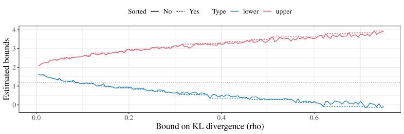
We first illustrate the estimators and confidence intervals we obtain under a fixed confounded data generating process. To be specific, we fix $\delta=0.5$ (hence $\rho=0.125$) to generate the data, and apply our procedure to the fixed dataset for a series of $\rho\in\{0.05,0.1,\dots,0.95,1.0\}$. We obtain $0.975$-lower confidence bound (LCB) for the lower bound of ATC and $0.975$-upper confidence bounds (UCB) for the upper bound of ATC (i.e., the bounds in (14)), which together form a $0.95$-CI for ATC under a hypothesized confounding level $\rho$. The results are plotted in Figure 3.

Without accounting for confounding, reweighting on the covariates tend to overestimate the ATC (indicated by the estimators for small $\rho$). The LCB crosses the ground truth at $\widehat{\rho}=0.1$; this can be viewed as a lower confidence bound for the true confounding level $\rho=0.125$ (we elaborate on this in the discussion when the ground truth is zero). Finally, the LCB hits zero at $\widehat{\rho}_{0}=0.65$; we can thus conclude with $0.95$-confidence that ATC is non-negative as long as the true confounding level does not exceed $\widehat{\rho}_{0}$.

Figure 3: The $0.975$-LCB for the lower bound of ATC (blue) and $0.975$-UCB for the upper bound of ATC (red), obtained from one run of our procedure on one dataset. Solid lines are the original estimators from our procedure, while dashed lines are sorted to ensure they are monotone in $\rho$. The black dashed line is the actual ATC.

5.3 Validity and sharpness

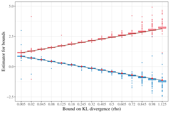
To show the validity and sharpness of our procedure, we first vary $\delta\in\{0.1,0.2,\dots,1.5\}$ in our data-generating process, and apply our procedure with the correct level $\rho=\delta^{2}/2$. Feeding the data into Algorithm 1 yields the estimator $\widehat{\mu}_{1,0}^{-}$ for the lower bound on $\mathbb{E}[Y(1){\,|\,}T=1]$; changing the observations to $Y(1)\leftarrow-Y(1)$, the negative of the output of Algorithm 1, denoted as $\widehat{\mu}_{1,0}^{+}$, is an estimator for the upper bound $\mu_{1,0}^{+}$. Based on the corresponding variance estimators $\widehat{\sigma}_{1,0,\pm}$, we construct the confidence interval for $\mathbb{E}[Y(1){\,|\,}T=0]$ as $\text{CI}_{\text{mean}}:=[\widehat{\mu}_{1,0}^{-}+z_{0.025}\widehat{\sigma}_{1,0,-}/\sqrt{n},\widehat{\mu}_{1,0}^{+}+z_{0.975}\widehat{\sigma}_{1,0,+}/\sqrt{n}]$; the confidence interval for $\mu_{1,0}^{-}$ is constructed as $\text{CI}_{\text{lower}}:=[\widehat{\mu}_{1,0}^{-}+z_{0.025}\widehat{\sigma}_{1,0,-}/\sqrt{n},\widehat{\mu}_{1,0}^{-}+z_{0.975}\widehat{\sigma}_{1,0,-}/\sqrt{n}]$, and similarly $\text{CI}_{\text{upper}}:=[\widehat{\mu}_{1,0}^{+}+z_{0.025}\widehat{\sigma}_{1,0,+}/\sqrt{n},\widehat{\mu}_{1,0}^{+}+z_{0.975}\widehat{\sigma}_{1,0,+}/\sqrt{n}]$ for $\mu_{1,0}^{+}$.

To obtain the ground truth of $\mu_{1,0}^{\pm}$ at each $\delta$, we evaluate the bounds on $\mathbb{E}[Y(1){\,|\,}X=x,T=0]$ for each $x$ by optimizing with a huge amount of samples from $\mathbb{P}_{Y(1){\,|\,}X=x,T=1}$; we then marginalize over $X{\,|\,}T=0$ to obtain an estimator the ground truth of $\mu_{1,0}^{\pm}$. For each $\delta$, this procedure is repeated and averaged over many runs to further reduce the random error.

The estimators for bounds of counterfactuals over $N=500$ runs for each $\rho$ are plotted in Figure 4 (they are evenly spaced on the $x$-axis). The simulation results show the sharpness and accuracy of our estimators: they are quite close to the ground truth, especially for small values of $\rho$; they get a bit conservative and have a larger variance when $\rho$ is as large as $1$. Interestingly, there are also a few outliers when $\rho$ is very small, and the estimators seem to be the most stable for an medium scale of $\rho$ (around 0.18 to 0.5). The actual value of $\mathbb{E}[Y(1){\,|\,}T=0]$ in our design, represented by the red triangles, are very close to the lower solid line, the ground truth of $\mu_{1,0}^{-}$; this means our simulation design is close to the worst case.

Figure 4: Boxplots for $\widehat{\mu}_{1,0}^{+}$ (red ones) and $\widehat{\mu}_{1,0}^{-}$ (blue ones) over $N=500$ replicates with each value of $\rho$. The solid lines are the ground truths of $\mu_{1,0}^{+}$ and $\mu_{1,0}^{-}$. The red triangles represent the actual value of $\mathbb{E}[Y(1){\,|\,}T=0]$ in our simulation setting.

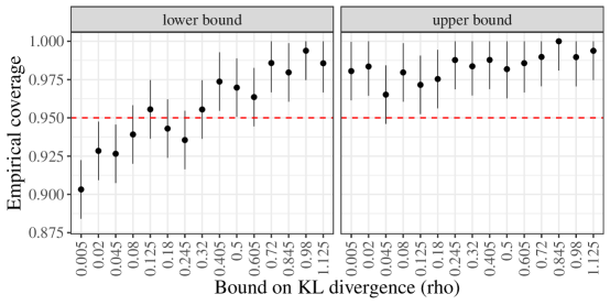
To further validate our inference procedure, we compute the empirical coverage of $\text{CI}_{\text{lower}}$ and $\text{CI}_{\text{upper}}$ for $\mu_{1,0}^{\pm}$ over $N=500$ runs. We also compute the ground truth of $\mathbb{E}[Y(1){\,|\,}T=0]$ under our design as a baseline, and compute the empirical coverage of $\text{CI}_{\text{mean}}$. They are plotted in Figure 5. Our empirical coverage is close to the nominal level $0.95$ in almost all settings, showing the validity of our inference procedure.

Figure 5: Empirical coverage for $\mu_{1,0}^{-}$ (left), $\mu_{1,0}^{+}$ (middle), and $\mathbb{E}[Y(1){\,|\,}T=0]$ (right). The short vertical segments are the C.I.s computed with $N=500$ replicates. The red dashed line is the nominal level $0.95$.

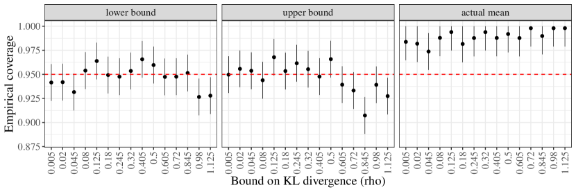
Figure 6 plots the empirical coverage of one-sided C.I.s for $\mu_{1,0}^{\pm}$, defined as $\text{CI}_{\text{lower}}^{\textrm{one-side}}:=[\widehat{\mu}_{1,0}^{-}+z_{0.05}\widehat{\sigma}_{1,0,-}/\sqrt{n},+\infty)$ and $\text{CI}_{\text{upper}}^{\textrm{one-side}}:=(-\infty,\widehat{\mu}_{1,0}^{+}+z_{0.95}\widehat{\sigma}_{1,0,+}/\sqrt{n}]$. Our theory shows that even though the ERM is off, these C.I.s still have valid asymptotic coverage; such robustness is also supported by empirical evidence.

Figure 6: Empirical coverage of one-sided C.I.s for $\mu_{1,0}^{-}$ (left), and $\mu_{1,0}^{+}$ (right). The short vertical segments are the C.I.s computed with $N=500$ replicates. The red dashed line is the nominal level $0.95$.

6 Discussion

In this work, we propose a new sensitivity model based on the $f$-divergence that characterizes the average effect of confounders on selection bias. Under the $f$-sensitivity model, we offer a scheme for the estimation and inference on the counterfactual and the ATE. We close the paper by a discussion on possible extensions.

Tightness.

As mentioned before, the optimal value of (11) is not necessarily the tightest lower bound for $\mathbb{E}[Y(1){\,|\,}T=0]$: the sharp one under $(f,\rho)$-selection condition is given by

$$\inf\Big{\{}\mathbb{E}^{\sup}\big{[}Y(1)\,\big{|}\,T=0\big{]}\colon{\mathbb{P}^{\sup}\in\mathcal{Q}_{1,0}}\Big{\}},$$

where $\mathcal{Q}_{1,0}$ is the identification set of all distributions that agree with the observed distribution and satisfy the $(f,\rho)$-selection condition. The constraints in (11) define a superset of $\mathcal{Q}_{1,0}$, potentially leading to conservativeness.

Using the exact characterization of $\mathcal{Q}_{1,0}$ provided in Proposition 5, we can represent the sharp lower (resp. upper) bound of $\mathbb{E}[Y(1){\,|\,}T=0]$ under the $(f,\rho)$-selection condition as the optimal value of

$$\mathop{\min(\text{resp.\leavevmode\nobreak\ }\max)}_{L(x)\textnormal{\leavevmode\nobreak\ measurable}}\leavevmode\nobreak\ \mathbb{E}\big{[}Y(1)L(X)\,\big{|}\,T=1\big{]}$$

s.t. $$\mathbb{E}[L(x){\,|\,}X=x,T=1]=r_{1,0}(x)$$

$$\mathbb{E}\big{[}f\big{(}L(x)/r_{1,0}(x)\big{)}\,\big{|}\,X=x,T=1\big{]}\leq\rho,\quad\mbox{for almost all }x.$$

$$\mathbb{E}\big{[}r_{1,0}(x)f\big{(}r_{1,0}(x)/L(x)\big{)}\,\big{|}\,X=x,T=1\big{]}\leq\rho,\quad\mbox{for almost all }x.$$

With the same argument, we can also develop the optimization problems for sharp bounds on the ATT and the ATC. Compared to the dual problems in Proposition 3, the additional constraints in the last line above leads to a dual form that is not as clean. Developing an efficient algorithm that solves this tight bound remains an interesting avenue for future research.

Sensitivity analysis.

In this paper, we have focused on conducting inference on the counterfactuals and treatment effects under the $(f,\rho)$-selection condition, with a prescribed confounding parameter $\rho$. Based on this, we can make robust causal conclusions and conduct sensitivity analysis by inverting the confidence intervals as follows. Suppose the goal is to detect if there is a nonzero ATE; we can consider a increasing sequence of $\rho$, and construct a level $1-\alpha$ confidence interval $\widehat{C}(\rho)$ for the ATE using the method introduced in this paper at each value of $\rho$; finally let $\widehat{\rho}$ be the smallest $\rho$ such that $C(\rho)$ contains zero. We can interprete the results as either there is a nonzero ATE, or there is a confounder as large as $\widehat{\rho}$ to explain away the observed treatment effects.

More rigorously, let $\rho^{*}$ denote the true confounding level and suppose the constructed confidence intervals $\widehat{C}(\rho)$ are nested in $\rho$: for any $\rho_{1}\leq\rho_{2}$, $\widehat{C}(\rho_{1})\subset\widehat{C}(\rho_{2})$. We then have

$$\limsup_{n\to\infty}\mathbb{P}(\mbox{ATE }=0,\rho^{*}<\widehat{\rho})\leq\limsup_{n\to\infty}\mathbb{P}(\mbox{ATE }\notin\widehat{C}(\rho^{*}))\leq\alpha,$$

if $\widehat{C}(\rho^{*})$ is an asymptotically valid confidence interval for the ATE. In words, when the ATE is indeed zero, $\widehat{\rho}$ is an asymptotic level-$(1-\alpha)$ confidence lower bound for $\rho^{*}$. Similar to the case of Jin et al., (2021), here only point-wise validity is necessary, i.e., we only need our CIs to be asymptotically valid for each fixed ground truth of $\rho$. Finally, we note that the monotonicity of the confidence intervals is satisfied with a reasonable estimation procedure; one can also force the confidence intervals to be monotone by enlarging some of them to conform to those for smaller values of $\rho$, without hurting the asymptotic validity.

Implications for the conditional average treatment effect (CATE).

The mothodology proposed in this paper also provides bounds on CATE under the $(f,\rho)$-selection condition. For example, the proof of Propositions 2 and 3 implies that a lower bound for $\mathbb{E}[Y(1){\,|\,}X=x,T=1]$ is given by the optimal value of

$$\min_{L\geq 0\textrm{ measurable}}\leavevmode\nobreak\ \mathbb{E}\big{[}Y(1)L{\,|\,}X=x,T=1\big{]}$$

$$s.t.\leavevmode\nobreak\ \mathbb{E}\big{[}L{\,|\,}T=1,X=x\big{]},$$

$$\mathbb{E}\bigg{[}f\Big{(}\frac{L}{r_{1,0}(x)}\Big{)}{\,|\,}X=x,T=1\bigg{]}\leq\rho.$$

The dual form of the above optimization problem is

$$\sup_{\alpha\geq 0,\eta\in\mathbb{R}}\leavevmode\nobreak\ -r_{1,0}(x)\cdot\mathbb{E}\bigg{[}\alpha f^{*}\Big{(}-\frac{Y(1)+\eta}{\alpha}\Big{)}+\eta+\alpha\rho\,\Big{|}\,X=x,T=1\bigg{]}.$$ (18)

Note that the optimizer $(\alpha^{*}(x),\eta^{*}(x))$ defined in (17) is exactly the optimizer of (18). In fact, $\widehat{\mu}(x):=\widehat{r}^{(j)}(x)\widehat{h}^{(j)}(x)$ where $\widehat{r}^{(j)},\widehat{h}^{(j)}$ are defined in Algorithm 1 is an estimator for the optimal objective in (18). These quantities are repeatedly estimated on distinct folds of data as intermediate steps of our procedure. While such sample splitting does not compromise the efficiency of inference due to the final averaging step, how to efficiently estimate these CATE bound functions with statistical guarantees might call for distinct considerations from ours. We leave this for future investigation.

Marginal $(f,\rho)$ selection condition.

We might even relax the per-$x$ uniform bound on the $f$-divergence in Definition 1 to a marginal fashion, so that the selection bias is controlled averaged over both $U$ and $X$. More formally, we might consider the constraint that

$$\int f\Big{(}\frac{\mathbb{P}(T=0{\,|\,}X=x,U)}{\mathbb{P}(T=1{\,|\,}X=x,U)}\frac{\mathbb{P}(T=1{\,|\,}X=x)}{\mathbb{P}(T=0{\,|\,}X=x)}\Big{)}\textnormal{d}\mathbb{P}_{U,X{\,|\,}T=1}\leq\rho.$$

In this setting, the odds ratio can be very large for a small proportion of $X{\,|\,}T=1$, but still controlled in the average sense. This type of marginal $(f,\rho)$-selection model leads to a larger class of distributional shifts than the $(f,\rho)$-selection condition here, and a different optimization problem for bounds on counterfactual means. Following similar arguments here, we see that the dual formulation, parallel to Proposition 3, can still be viewed as a risk minimization problem; however, the risk function would involve the unknown $X$-shift $r_{1,0}$, which might make the estimation and inference more complicated. The estimation and inference under this marginal $f$-sensitivity model is an ongoing work.

7 Acknowledgement

The authors thank Emmanuel Candès, Kevin Guo and Dominik Rothenhäusler for helpful discussions. Z. R. was partially supported by ONR grant N00014-20-1-2337, and NIH grants R56HG010812, R01MH113078 and R01MH123157.

Appendix A Proofs for identification sets

A.1 Proof of Proposition 1

Here we prove a stronger result that directly implies Proposition 1. The following proposition is a tight characterization of the identification set induced by the $f$-sensitivity models.

Proposition 5.

Let $(X,Y(0),Y(1),U,T)\sim\mathbb{P}^{\sup}$ be the true unknown super-population over all random variables of interest. Let $\mathcal{P}$ be the set of all distributions over $(X,Y(0),Y(1),U,T)$. Let $\mathbb{P}^{\textnormal{obs}}_{X,Y,T}$ be the joint distribution of all observable random variables $(X,Y,T)$. Let $t\in\{0,1\}$. Define $\mathcal{Q}_{t,1-t}$ as the set of all counterfactual distributions that agrees with the observables and satisfies the $(f,\rho)$ selection condition, i.e.,

$$\mathcal{Q}_{t,1-t}=\big{\{}\mathbb{P}_{X,Y(t){\,|\,}T=1-t}\colon\mathbb{P}\in\mathcal{P},\leavevmode\nobreak\ \mathbb{P}_{X,Y,T}=\mathbb{P}^{\textnormal{obs}}_{X,Y,T},\leavevmode\nobreak\ \mathbb{P}\,\text{satisfies Definition\leavevmode\nobreak\ \ref{def:cond}}\,\big{\}}.$$

Then $\mathbb{P}^{\sup}_{X,Y(t){\,|\,}T=1-t}\in\mathcal{Q}_{t,1-t}$, and

$$\mathcal{Q}_{t,1-t}=\Bigg{\{}\mathbb{Q}\colon\frac{{\,\mathrm{d}}\mathbb{Q}_{X}}{{\,\mathrm{d}}\mathbb{P}_{X{\,|\,}T=t}^{\textnormal{obs}}}(x)=r_{t,1-t}(x),\leavevmode\nobreak\ D_{f}\big{(}\mathbb{Q}_{Y{\,|\,}X=x}\leavevmode\nobreak\ \big{\|}\leavevmode\nobreak\ \mathbb{P}_{Y{\,|\,}X=x,T=t}^{\textnormal{obs}}\big{)}\leq\rho,\leavevmode\nobreak\ \text{for }\mathbb{P}^{\textnormal{obs}}_{X{\,|\,}T=t}\text{-almost all }x,$$

$$\quad D_{f}\big{(}\mathbb{Q}_{Y^{\textnormal{obs}}{\,|\,}X=x,T=t}\leavevmode\nobreak\ \big{\|}\leavevmode\nobreak\ \mathbb{Q}_{Y{\,|\,}X=x}\big{)}\leq\rho,\leavevmode\nobreak\ \text{for }\mathbb{Q}_{X}\text{-almost all }x\Bigg{\}},$$

where $r_{1,0}(x)=\frac{(1-e(x))p_{1}}{e(x)(1-p_{1})}$, $r_{0,1}(x)=\frac{e(x)(1-p_{1})}{(1-e(x))p_{1}}$, and $e(x)=\mathbb{P}^{\textnormal{obs}}(T=1{\,|\,}X=x)$, $p_{1}=\mathbb{P}^{\textnormal{obs}}(T=1)$.

Proof of Proposition 5.

Fix $t=1$. For any $\mathbb{P}_{X,Y(1){\,|\,}T=0}\in\mathcal{Q}_{1,0}$, since $\mathbb{P}_{X,Y,T}=\mathbb{P}^{\rm obs}_{X,Y,T}$,

$$\frac{{\,\mathrm{d}}\mathbb{P}_{X{\,|\,}T=0}}{{\,\mathrm{d}}\mathbb{P}^{\rm obs}_{X{\,|\,}T=1}}=\frac{{\,\mathrm{d}}\mathbb{P}_{X{\,|\,}T=0}}{{\,\mathrm{d}}\mathbb{P}_{X{\,|\,}T=1}}=r_{1,0}(x).$$

By Lemma 1, $D_{f}\big{(}\mathbb{P}_{X,Y(1){\,|\,}T=0}\leavevmode\nobreak\ \big{\|}\leavevmode\nobreak\ \mathbb{P}_{X,Y(1){\,|\,}T=1}\big{)}\leq\rho.$ On the other hand,

$$D_{f}\big{(}\mathbb{P}_{Y(1){\,|\,}X,T=1}\leavevmode\nobreak\ \|\leavevmode\nobreak\ \mathbb{P}_{Y(1){\,|\,}X,T=0}\big{)}\leq D_{f}\big{(}\mathbb{P}_{Y(1),U{\,|\,}X,T=1}\leavevmode\nobreak\ \|\leavevmode\nobreak\ \mathbb{P}_{Y(1),U{\,|\,}X,T=0}\big{)}$$

$$= \mathbb{E}_{\mathbb{P}_{Y(1),U{\,|\,}X,T=0}}\bigg{[}f\Big{(}\frac{{\,\mathrm{d}}\mathbb{P}_{Y(1),U{\,|\,}X,T=1}}{{\,\mathrm{d}}\mathbb{P}_{Y(1),U{\,|\,}X,T=0}}\Big{)}\bigg{]}$$

$$= \mathbb{E}_{U{\,|\,}X,T=0}\bigg{[}f\Big{(}\frac{\mathbb{P}(T=1{\,|\,}X,U)}{\mathbb{P}(T=0{\,|\,}X,U)}\cdot\frac{\mathbb{P}(T=0{\,|\,}X)}{\mathbb{P}(T=1{\,|\,}X)}\Big{)}\bigg{]}\leq\rho,$$

where the last inequality is due to the $(f,\rho)$-selection condition. Combining the above, we establish the “$\subset$” direction. It remains to prove the reverse. We show the proof for the case of $t=1$ here, and the $t=0$ case follows from similar arguments.

Given any $Q\in\mathcal{Q}_{1,0}$, we aim to find a distribution $\mathbb{P}^{\rm sup}$ over $(X,Y(0),Y(1),U,T)$ such that

• $(Y(1),Y(0))\rotatebox[origin={c}]{90.0}{$\models$}T{\,|\,}X,U$

• $\mathbb{P}^{\rm sup}$ is compatible with $\mathbb{P}^{\rm obs}_{X,T,Y}$;

• $\mathbb{P}^{\rm sup}$ satisfies the $(f,\rho)$-selection condition;

• $\mathbb{P}^{\rm sup}_{X,Y(1){\,|\,}T=0}(x,y)=Q(x,y)$.

To construct $\mathbb{P}^{\rm sup}$, we first set $\mathbb{P}^{\rm sup}_{X,T}=\mathbb{P}^{\rm obs}_{X,T}$. Then we specify the distribution of $Y(1){\,|\,}X,T$ via

$$\mathbb{P}^{\rm sup}_{Y(1){\,|\,}X,T=1}=\mathbb{P}^{\rm obs}_{Y{\,|\,}X,T=1},\quad\mathbb{P}^{\rm sup}_{Y(1){\,|\,}X,T=0}=Q_{Y{\,|\,}X}.$$

So far the joint distribution of $(X,T,Y(1))$ has been determined. We let $U=Y(1)$ be the unobserved confounder. Finally, the distribution of $Y(0){\,|\,}X,T,Y(1),U$ is specified via

$$\mathbb{P}^{\rm sup}_{Y(0){\,|\,}X,T,Y(1),U}=\mathbb{P}^{\rm sup}_{Y(0){\,|\,}X}=\mathbb{P}^{\rm obs}_{Y{\,|\,}X,T=0}.$$

Having constructed $\mathbb{P}^{\rm sup}$, we proceed the check that it satisfies the conditions. Conditional on $X$ and $U$, $Y(1)$ becomes deterministic and the distribution of $Y(0)$ only depends on $X$. Hence $(Y(1),Y(0))\rotatebox[origin={c}]{90.0}{$\models$}T{\,|\,}X,U$. By construction, it is straightforward to see that $\mathbb{P}^{\rm sup}$ is compatible with $\mathbb{P}^{\rm obs}_{X,T,Y}$. For any $x$, again by the construction of $\mathbb{P}^{\rm sup}$,

$$\mathbb{E}_{\mathbb{P}^{\rm sup}_{Y(1){\,|\,}X=x,T=1}}\bigg{[}f\Big{(}\frac{{\,\mathrm{d}}\mathbb{P}^{\rm sup}_{Y(1){\,|\,}X=x,T=0}}{{\,\mathrm{d}}\mathbb{P}^{\rm\sup}_{Y(1){\,|\,}X=x,T=1}}\Big{)}\bigg{]}=\mathbb{E}_{\mathbb{P}^{\rm obs}_{Y{\,|\,}X=x,T=1}}\bigg{[}f\Big{(}\frac{{\,\mathrm{d}}Q_{Y{\,|\,}X=x}}{{\,\mathrm{d}}\mathbb{P}^{\rm\textnormal{obs}}_{Y{\,|\,}X=x,T=1}}\Big{)}\bigg{]}=D_{f}\big{(}Q_{Y{\,|\,}X=x}\leavevmode\nobreak\ \|\leavevmode\nobreak\ \mathbb{P}^{\rm obs}_{Y{\,|\,}X=x,T=1}\big{)}\leq\rho,$$

where the last inequality is due to the definition of $\mathcal{Q}$. On the other hand,

$$\frac{{\,\mathrm{d}}\mathbb{P}^{\rm sup}_{Y(1){\,|\,}X=x,T=0}}{{\,\mathrm{d}}\mathbb{P}^{\rm\sup}_{Y(1){\,|\,}X=x,T=1}}=\frac{{\,\mathrm{d}}\mathbb{P}^{\rm sup}_{Y(1),T=0{\,|\,}X=x}}{{\,\mathrm{d}}\mathbb{P}^{\rm\sup}_{Y(1),T=1{\,|\,}X=x}}\cdot\frac{\mathbb{P}^{\rm sup}(T=1{\,|\,}X=x)}{\mathbb{P}^{\rm sup}(T=0{\,|\,}X=x)}= \frac{\mathbb{P}^{\sup}(T=0{\,|\,}Y(1),X=x)}{\mathbb{P}^{\rm sup}(T=1{\,|\,}Y(1),X=x)}\cdot\frac{\mathbb{P}^{\rm sup}(T=1{\,|\,}X=x)}{\mathbb{P}^{\rm sup}(T=0{\,|\,}X=x)}$$

$$= \frac{\mathbb{P}^{\rm sup}(T=0{\,|\,}U,X=x)}{\mathbb{P}^{\rm\sup}(T=1{\,|\,}U,X=x)}\cdot\frac{\mathbb{P}^{\rm sup}(T=1{\,|\,}X=x)}{\mathbb{P}^{\rm sup}(T=0{\,|\,}X=x)},$$

where the last equality is because $U=Y(1)$ under $\mathbb{P}^{\rm sup}$. Combing the above, we have

$$\mathbb{E}_{\mathbb{P}^{\rm sup}_{U{\,|\,}X=x,T=1}}\bigg{[}f\Big{(}\frac{\mathbb{P}^{\rm sup}(T=0{\,|\,}U,X=x)}{\mathbb{P}^{\rm\sup}(T=1{\,|\,}U,X=x)}\cdot\frac{\mathbb{P}^{\rm sup}(T=1{\,|\,}X=x)}{\mathbb{P}^{\rm sup}(T=0{\,|\,}X=x)}\Big{)}\bigg{]}\leq\rho.$$

Similarly,

$$\mathbb{E}_{\mathbb{P}^{\rm sup}_{U{\,|\,}X=x,T=0}}\bigg{[}f\Big{(}\frac{\mathbb{P}^{\rm sup}(T=1{\,|\,}U,X=x)}{\mathbb{P}^{\rm\sup}(T=0{\,|\,}U,X=x)}\cdot\frac{\mathbb{P}^{\rm sup}(T=0{\,|\,}X=x)}{\mathbb{P}^{\rm sup}(T=1{\,|\,}X=x)}\Big{)}\bigg{]}\leq\mathbb{E}_{\mathbb{P}^{\rm sup}_{Y(1){\,|\,}X=x,T=0}}\bigg{[}f\Big{(}\frac{{\,\mathrm{d}}\mathbb{P}^{\rm sup}_{Y(1){\,|\,}X=x,T=1}}{{\,\mathrm{d}}\mathbb{P}^{\rm\sup}_{Y(1){\,|\,}X=x,T=0}}\Big{)}\bigg{]}$$

$$= \mathbb{E}_{\mathbb{P}^{\rm obs}_{Y{\,|\,}X=x,T=0}}\bigg{[}f\Big{(}\frac{{\,\mathrm{d}}\mathbb{P}^{\textnormal{obs}}_{Y{\,|\,}X=x,T=1}}{{\,\mathrm{d}}Q_{Y{\,|\,}X=x}}\Big{)}\bigg{]}=D_{f}\big{(}\mathbb{P}^{\textnormal{obs}}_{Y{\,|\,}X=x,T=1}\leavevmode\nobreak\ \|\leavevmode\nobreak\ Q_{Y{\,|\,}X=x}\big{)}\leq\rho.$$

Therefore, the super population $\mathbb{P}^{\rm sup}$ satisfies the $(f,\rho)$-selection condition. By construction, $\mathbb{P}^{\rm sup}_{Y(1){\,|\,}X,T=0}=Q_{Y{\,|\,}X}$. It remains to show that $\mathbb{P}^{\rm sup}_{X{\,|\,}T=0}=Q_{X}$. For any measurable set $A$,

$$\mathbb{P}^{\rm sup}(X\in A{\,|\,}T=0)= \mathbb{E}^{\rm sup}\bigg{[}\frac{{\,\mathrm{d}}\mathbb{P}^{\rm sup}_{X{\,|\,}T=0}}{{\,\mathrm{d}}\mathbb{P}^{\rm sup}_{X{\,|\,}T=1}}\cdot\mathds{1}\{X\in A\}\,\Big{|}\,T=1\bigg{]}=\mathbb{E}^{\rm sup}\bigg{[}\frac{{\,\mathrm{d}}\mathbb{P}^{\rm obs}_{X{\,|\,}T=0}}{{\,\mathrm{d}}\mathbb{P}^{\rm obs}_{X{\,|\,}T=1}}\cdot\mathds{1}\{X\in A\}\,\Big{|}\,T=1\bigg{]}$$

$$= \mathbb{E}^{\rm sup}\Big{[}r_{1,0}(X)\cdot\mathds{1}\{X\in A\}\,\Big{|}\,T=1\Big{]}=\mathbb{E}^{\rm sup}\bigg{[}\frac{{\,\mathrm{d}}Q_{X}}{{\,\mathrm{d}}\mathbb{P}^{\rm sup}_{X{\,|\,}T=1}}\cdot\mathds{1}\{X\in A\}\,\Big{|}\,T=1\bigg{]}=Q(X\in A).$$

Since the above holds for any measuable set $A$, $\mathbb{P}_{X{\,|\,}T=0}=Q_{X}$.

Finally, switching the role of $1$ and $0$ completes the proof.

∎

Appendix B Deferred details and discussions

B.1 Proof of Proposition 4

Given $X=x$, suppose instead $\alpha^{*}(x)=0$. We consider the following two cases:

• If $\eta^{*}(x)<-\underline{y}(x)$, then

  $$\lim\!\inf_{\alpha\rightarrow 0}\mathbb{E}\bigg{[}\alpha f^{*}\Big{(}\frac{Y(1)+\eta^{*}(x)}{-\alpha}\Big{)}+\eta^{*}(x)+\alpha\rho\,\big{|}\,X=x,T=1\bigg{]}$$

  $$= \lim\!\inf_{\alpha\rightarrow 0}\mathbb{E}\bigg{[}\alpha f^{*}\Big{(}\frac{Y(1)+\eta^{*}(x)}{-\alpha}\Big{)}\mathds{1}\big{\{}Y(1)\leq-\eta^{*}(x)\big{\}}$$

  $$\qquad+\alpha f^{*}\Big{(}\frac{Y(1)+\eta^{*}(x)}{-\alpha}\Big{)}\mathds{1}\big{\{}Y(1)>-\eta^{*}(x)\big{\}}\,\big{|}\,X=x,T=1\bigg{]}+\eta^{*}(x)+\alpha\rho$$

  $$\stackrel{{\scriptstyle\rm(a)}}{{\geq}} \lim\!\inf_{\alpha\rightarrow 0}\mathbb{E}\bigg{[}\alpha f^{*}\Big{(}\frac{Y(1)+\eta^{*}(x)}{-\alpha}\Big{)}\mathds{1}\big{\{}Y(1)\leq-\eta^{*}(x)\big{\}}-\alpha L\,\Big{|}\,X=x,T=1\bigg{]}$$

  $$\qquad+\lim\!\inf_{\alpha\rightarrow 0}\bigg{[}\alpha f^{*}\Big{(}\frac{Y(1)+\eta}{-\alpha}\Big{)}\mathds{1}\big{\{}Y(1)>-\eta^{*}(x)\big{\}}-\alpha L\,\big{|}\,X=x,T=1\bigg{]}+\eta^{*}(x)$$

  $$\stackrel{{\scriptstyle\rm(b)}}{{\geq}} +\infty,$$

  where step (a) uses the fact that $\lim\!\inf_{n\rightarrow\infty}a_{n}+b_{n}\geq\lim\!\inf_{n\rightarrow\infty}a_{n}+\lim\!\inf_{n\rightarrow\infty}b_{n}$ and step (b) follows from Fatou’s lemma and the condition that $f^{*}(x)/x\rightarrow\infty$ when $x\rightarrow\infty$.

• If $\eta^{*}(x)\geq-\underline{y}(x)$, then

  $$\lim_{\alpha\rightarrow 0}\mathbb{E}\bigg{[}\alpha f^{*}\Big{(}\frac{Y(1)+\eta^{*}(x)}{-\alpha}\Big{)}+\eta^{*}(x)+\alpha\rho\,\big{|}\,X=x,T=1\bigg{]}$$

  $$= \lim_{\alpha\rightarrow 0}\mathbb{E}\bigg{[}\alpha f^{*}\Big{(}\frac{Y(1)+\eta^{*}(x)}{-\alpha}\Big{)}\mathds{1}\big{\{}Y(1)\geq{\textnormal{ess}}\!\inf Y(1)\big{\}}+\alpha\rho\,\big{|}\,X=x,T=1\bigg{]}+\eta^{*}(x)$$

  $$\stackrel{{\scriptstyle\rm(a)}}{{=}} \mathbb{E}\bigg{[}\lim_{\alpha\rightarrow 0}\alpha f^{*}\Big{(}\frac{Y(1)+\eta^{*}(x)}{-\alpha}\Big{)}\mathds{1}\big{\{}Y(1)\geq{\textnormal{ess}}\!\inf Y(1)\big{\}}+\alpha\rho\,\big{|}\,X=x,T=1\bigg{]}+\eta^{*}(x)$$

  $$\stackrel{{\scriptstyle\rm(b)}}{{=}} \eta^{*}(x).$$

  Above, step (a) is due to the fact that $f^{*}(x)$ is bounded when $x\leq 0$ and the dominated convergence theorem; step (b) is because $f^{*}(x)/x\rightarrow 0$ as $x\rightarrow-\infty$.

Combining the two cases above, we conclude that $\eta^{*}(x)=-\underline{y}(x)$ and the optimal value of the dual problem is $-\underline{y}(x)$. By the strong duality, the optimal value of the primal objective function is $\mathbb{E}\big{[}r_{1,0}(X)\underline{y}(X){\,|\,}T=1\big{]}$. As an implication, there exists a feasible $L(x,y)$ such that $\mathbb{E}[Y(1)L(X,Y(1)){\,|\,}T=1]=\mathbb{E}\big{[}r_{1,0}(X)\underline{y}(X){\,|\,}T=1\big{]}$. Let $\mathbb{Q}_{Y{\,|\,}X=x}$ denote the measure induced by $L(x,y)$:

$$\frac{{\,\mathrm{d}}\mathbb{Q}_{Y{\,|\,}X=x}}{{\,\mathrm{d}}\mathbb{P}_{Y(1){\,|\,}X=x,T=1}}(y)=\frac{L(x,y)}{r_{1,0}(x)}.$$

This is a valid transformation of measure because $L(x,y)$ is feasible. Then $Y(1)=\underline{y}(X)$ a.s. under $\mathbb{Q}_{Y{\,|\,}X}$. Consequently,

$$1=\mathbb{Q}\big{(}Y(1)=\underline{y}(X){\,|\,}X=x\big{)}=\mathbb{E}\bigg{[}\frac{L\big{(}x,\underline{y}(x)\big{)}}{r_{1,0}(x)}\cdot\mathds{1}\big{\{}Y(1)=\underline{y}(x)\big{\}}\,\Big{|}\,X=x,T=1\bigg{]}=\frac{L(x,\underline{y}(x))}{r_{1,0}(x)}\cdot\bar{p}(x),$$

$$0=L(x,Y(1))\cdot\mathds{1}\{Y(1)>\underline{y}(x)\},\leavevmode\nobreak\ \text{a.s. under }\mathbb{P}_{Y(1){\,|\,}X=x,T=1}.$$

Again since $L$ is feasible,

$$\rho\geq\mathbb{E}\bigg{[}f\Big{(}\frac{L(x,Y(1))}{r_{1,0}(x)}\Big{)}\,\Bigg{|}\,X=x,T=1\bigg{]}=\bar{p}(x)\cdot f\Big{(}\frac{1}{\bar{p}(x)}\Big{)}+\big{(}1-\bar{p}(x)\big{)}\cdot f(0).$$

This is a contradiction to the condition. Hence $\alpha^{*}(x)>0$.

B.2 Discussions on Assumption 2 on sieve estimation

We provide additional discussion on Assumption 2 for sieve estimators in the context of $(X,Y(1)){\,|\,}T=1$. In particular, we first justify the smoothness of the optimizers when the conditional distributions are sufficiently smooth. We then verify the technical conditions for two choices of $f$-divergences: KL-divergence and $\chi^{2}$-divergence. Then we discuss some considerations of relaxing the conditions with implementations in practice.

Smoothness of the optimizers.

We first provide some justifications for assuming the optimizers are continuously differentiable. By the strong convexity of $f$, its conjugate $f^{*}$ is continuous, hence without loss of generality we always assume the differentiation and expectation are exchangeable. We also assume the conjugate $f^{*}$ is sufficiently smooth, which is the case for many popular choices of $f$-divergence. As we discussed in Proposition 4, under mild conditions, the optimizers $(\alpha^{*}(x),\eta^{*}(x))$ lies in the interior of $\mathbb{R}^{+}\times\mathbb{R}$. The optimizers are thus the solutions to

$$\big{(}\alpha^{*}(x),\eta^{*}(x)\big{)}=\textrm{argzero}\leavevmode\nobreak\ \nabla_{a,b}\bigg{\{}a\mathbb{E}\Big{[}f^{*}\big{(}{\textstyle\frac{Y(1)+b}{-a}}\big{)}\,\Big{|}\,X=x,T=1\Big{]}+b+a\rho\bigg{\}},$$

where the right-hand side takes the form

$$F(a,b,x):=\mathbb{E}\big{[}g(Y(1),a,b)\,\big{|}\,X=x,T=1\big{]}\in\mathbb{R}^{2}$$

for some differentiable or smooth function $g$ decided by $f^{*}$ and its derivative $(f^{*})^{\prime}$. Thus $F(a,b,x)$ is smooth in $(a,b)$ when $f^{*}$ is sufficiently smooth. Now let us assume the conditional distribution $\mathbb{P}_{Y(1){\,|\,}X=x,T=1}$ is smooth; for example, for some $h\in\mathcal{X}$, $\mathbb{P}_{Y(1){\,|\,}X=x+th,T=1}=\mathbb{P}_{Y(1){\,|\,}X=x,T=1}+t\cdot\mathbb{P}_{h}$ for some measure $\mathbb{P}_{h}$ on $\mathcal{Y}$; and similar for higher-order expansions. This is a reasonable assumption if we are willing to assume that the conditional distributions of $Y(1)$ are close for similar covariates. Concretely, such condition holds when $Y(1){\,|\,}X=x,T=1$ is a normal distribution with homoskedastic noise and a smooth mean function, or heteroskedastic noise with a smooth mean function and smooth standard deviation function, etc. When the conditional distributions are smooth in $x$, the function $F(a,b,x)$ is also smooth in $x$ by the linearity of conditional expectation. Finally, if the derivatives with respect to $a,b$ is always invertible (which is the case under mild conditions for the examples we discuss shortly) and smooth, invoking the Implicit Function Theorem (Rudin et al.,, 1976), the minimizer can be smooth in $x$.

KL-divergence.

A popular choice for the function $f$ is $f(x)=x\log x$, which leads to the KL-divergence (Kullback and Leibler,, 1951). The dual function in this case is $f^{*}(y)=e^{y-1}$, and the loss function becomes

$$\ell(\theta,x,y)=\alpha(x)e^{\frac{y+\eta(x)}{-\alpha(x)}-1}+\eta(x)+\alpha(x)\rho.$$

The conditional expectation is

$$\mathbb{E}\big{[}\ell((a,b),x,Y(1))\,\big{|}\,X=x,T=1\big{]}=a\mathbb{E}\big{[}e^{\frac{Y(1)-b}{-a}-1}\,\big{|}\,X=x,T=1\big{]}+b+a\rho.$$

We first look at the strong convexity assumption. The conditional expectation is twice differentiable, with

$$\nabla_{a}^{2}\mathbb{E}\big{[}\ell((a,b),x,Y(1))\,\big{|}\,X=x,T=1\big{]}=\frac{1}{a^{3}}\mathbb{E}\Big{[}\big{(}Y(1)+b\big{)}^{2}e^{\frac{Y(1)+b}{-a}-1}\,\Big{|}\,X=x,T=1\Big{]},$$

$$\nabla_{b}^{2}\mathbb{E}\big{[}\ell((a,b),x,Y(1))\,\big{|}\,X=x,T=1\big{]}=\frac{1}{a}\mathbb{E}\Big{[}e^{\frac{Y(1)+b}{-a}-1}\,\Big{|}\,X=x,T=1\Big{]},$$

$$\nabla_{a,b}^{2}\mathbb{E}\big{[}\ell((a,b),x,Y(1))\,\big{|}\,X=x,T=1\big{]}=-\frac{1}{a^{2}}\mathbb{E}\Big{[}\big{(}Y(1)+b\big{)}e^{\frac{Y(1)+b}{-a}-1}\,\Big{|}\,X=x,T=1\Big{]}.$$

Therefore, a simple calculation shows that as long as $Y(1)$ is not deterministic at $(\alpha^{*}(x),\beta^{*}(x))$, the Hessian matrix is non-singular. Also, if the underlying distribution $\mathbb{P}_{Y(1){\,|\,}X=x,T=1}$ is continuous in $x$, the above derivatives, hence the eigenvalues of the Hessian matrix is continuous; since $\mathcal{X}$ is compact, there exists a positive uniform lower bound for the smallest eigenvalue of the Hessian matrix, leading to strong convexity.

We then consider the continuity condition $|\ell(\theta,x,y)-\ell(\theta^{*},x,y)|\leq\bar{\ell}(x,y)\|\theta(x)-\theta^{*}(x)\|_{2}$ for $\|\theta(x)-\theta^{*}(x)\|_{2}<\epsilon$ for some sufficiently small $\epsilon>0$, where $\|\theta(x)-\theta^{*}(x)\|_{2}$ is the Euclidean norm, and $\sup_{x\in\mathcal{X}}\mathbb{E}[\bar{\ell}(x,Y(1))^{2}{\,|\,}X=x,T=1]<M$ for some constant $M>0$. By Taylor expansion, we have

$$\ell(\theta,x,y)-\ell(\theta^{*},x,y)=\nabla_{\theta}\ell(\widetilde{\theta},x,y)\big{(}\theta^{*}(x)-\theta(x)\big{)},$$

where $\widetilde{\theta}(x)$ lies between $\theta(x)$ and $\theta^{*}(x)$. We note that $\nabla_{\theta}$ is also a smooth function of $\theta$, and the gradient is uniform bounded for $\theta(x)$ within a neighborhood of $\theta^{*}(x)$ in terms of Euclidean $L_{2}$-norm. In particular,

$$\frac{\partial}{\partial a}\ell((a,b),x,y)=\big{(}1-{\textstyle\frac{y+b}{a}}\big{)}e^{\frac{y+b}{-a}-1}+\rho,\quad\frac{\partial}{\partial b}\ell((a,b),x,y)=1-e^{\frac{y+b}{-a}-1}.$$

For any $\|(a,b)-\theta^{*}(x)\|_{2}\leq\epsilon$ for sufficiently small $\epsilon$, we can take $\bar{\ell}(x,y)$ as the uniform upper bound of the Euclidean norm of the gradient, which has finite second moment if $Y(1)$ is not too heavy-tailed.

Finally, the last condition is that there exists a constant $C_{1}$ such that $\mathbb{E}[\ell(\theta,X,Y(1))-\ell(\theta^{*},X,Y(1)){\,|\,}T=1]\leq C_{1}\|\theta-\theta^{*}\|_{L_{2}(\mathbb{P}_{\cdot{\,|\,}T=1})}^{2}$ when $\theta\in\Lambda_{c}^{p}(\mathcal{X})\times\Lambda_{c}^{p}(\mathcal{X})$ and $\|\theta-\theta^{*}\|_{L_{2}(\mathbb{P}_{\cdot{\,|\,}T=1})}$ is sufficiently small. Similar to arguments in the proof of Theorem 1, sufficiently small $\|\theta-\theta^{*}\|_{L_{2}(\mathbb{P}_{\cdot{\,|\,}T=1})}$ implies sufficiently small $\|\theta-\theta^{*}\|_{\infty}$ for this function class. Therefore, we can consider $\theta\in\Lambda_{c}^{p}(\mathcal{X})\times\Lambda_{c}^{p}(\mathcal{X})$ such that $\|\theta-\theta^{*}\|_{\infty}$ is sufficiently small. With a taylor expansion of the conditional expectation of the risk at $(\alpha^{*}(x),\eta^{*}(x))$, we have

$$\mathbb{E}\big{[}\ell(\theta,x,Y(1))\,\big{|}\,X=x,T=1\big{]}-\mathbb{E}\big{[}\ell(\theta^{*},x,Y(1))\,\big{|}\,X=x,T=1\big{]}$$

$$=1/2\cdot\nabla_{\theta}^{2}\mathbb{E}\big{[}\ell(\widetilde{\theta},x,Y(1))\,\big{|}\,X=x,T=1\big{]}[\theta(x)-\theta*(x),\theta(x)-\theta^{*}(x)]$$

since the gradient is zero, where $\widetilde{\theta}(x)$ lies between $\theta(x)$ and $\theta^{*}(x)$. Previous derivations have shown that the Hessian is continuous; also, by the compactness of $\mathcal{X}$ and continuity of $\theta^{*}(x)$, there is a uniform lower bound $\epsilon>0$ for $\alpha^{*}(x)$. Thus, when $\|\theta-\theta^{*}\|_{\infty}$ is sufficiently small, the Hessian is also bounded. Again by the compactness of $\mathcal{X}$, this bound can be taken to be uniform for $x\in\mathcal{X}$, which leads to the desired condition.

$\chi^{2}$-divergence.

Another popular choice is $f(x)=(x-1)^{2}$, so that $f^{*}(y)=\frac{1}{4}((y+2)_{+}^{2}-1)$. The conjugate function is a quadratic function on $[-2,\infty)$ and zero on $(-\infty,-2]$, with continuous gradient $(f^{*})^{\prime}(y)=(\frac{s}{2}+1)_{+}$, and second-order derivative $(f^{*})^{\prime\prime}(y)=\frac{1}{2}\mathds{1}\{y>-2\}$; the latter is almost-everywhere (under Lebesgue measure) except $y=2$. We now proceed to verify the conditions. The loss function is

$$\ell(\theta,x,y)=\frac{\alpha(x)}{4}\Big{[}\Big{(}\frac{y+\eta(x)}{-\alpha(x)}+1\Big{)}_{+}^{2}-1\Big{]}+\eta(x)+\alpha(x)\rho.$$

Assuming $Y(1)$ does not have point measure, the differentiation and expectation are exchangeable, and

$$\nabla_{a}^{2}\mathbb{E}\big{[}\ell((a,b),x,Y(1))\,\big{|}\,X=x,T=1\big{]}=\frac{1}{2a^{3}}\mathbb{E}\Big{[}\big{(}Y(1)+b\big{)}^{2}\mathds{1}\{\textstyle{\frac{Y(1)+b}{-a}}>-2\}\,\Big{|}\,X=x,T=1\Big{]},$$

$$\nabla_{b}^{2}\mathbb{E}\big{[}\ell((a,b),x,Y(1))\,\big{|}\,X=x,T=1\big{]}=\frac{1}{2a}\mathbb{E}\Big{[}\mathds{1}\{\textstyle{\frac{Y(1)+b}{-a}}>-2\}\,\Big{|}\,X=x,T=1\Big{]},$$

$$\nabla_{a,b}^{2}\mathbb{E}\big{[}\ell((a,b),x,Y(1))\,\big{|}\,X=x,T=1\big{]}=-\frac{1}{2a^{2}}\mathbb{E}\Big{[}\big{(}Y(1)+b\big{)}\mathds{1}\{\textstyle{\frac{Y(1)+b}{-a}}>-2\}\,\Big{|}\,X=x,T=1\Big{]}.$$

Also, the gradient is given by

$$\nabla_{a}\mathbb{E}\big{[}\ell((a,b),x,Y(1))\,\big{|}\,X=x,T=1\big{]}=\mathbb{E}\Big{[}\big{(}{\textstyle\frac{Y(1)+b}{-2a}+1}\big{)}_{+}^{2}-1+{\textstyle\frac{Y(1)+b}{a}}\big{(}{\textstyle\frac{Y(1)+b}{-2a}+1}\big{)}_{+}\,\Big{|}\,X=x,T=1\Big{]}+\rho,$$

$$\nabla_{b}\mathbb{E}\big{[}\ell((a,b),x,Y(1))\,\big{|}\,X=x,T=1\big{]}=-\mathbb{E}\Big{[}\big{(}{\textstyle\frac{Y(1)+b}{-2a}+1}\big{)}_{+}\,\Big{|}\,X=x,T=1\Big{]}+1,$$

which are both zero at $(a,b)=(\alpha^{*}(x),\eta^{*}(x))$. The form of the loss function implies that $\alpha^{*}(x)>0$ for almost all $x$; hence there is a uniform lower bound $\epsilon>0$ by the compactness of $\mathcal{X}$. By Cauchy-Schwarz inequality, the Hessian at $(a,b)=(\alpha^{*}(x),\eta^{*}(x))$ is positive $\mathbb{P}(\frac{Y(1)+\eta^{*}(x)}{-\alpha^{*}(x)}>-2{\,|\,}X=x,T=1)=0$ or $(Y(1)+\eta^{*}(x)-c(x))\mathds{1}\{\textstyle{\frac{Y(1)+\eta^{*}(x)}{-a}}>-2\}=0$ almost surely for some $c(x)\in\mathbb{R}$. By the optimality condition, the former is impossible, and the latter is also impossible if $Y(1)$ is not deterministic conditional on $X=x$. Thus, as long as $Y(1){\,|\,}X=x$ is not deterministic for almost all $x$, the Hessian is positive definite for all $x\in\mathcal{X}$. By compactness of $\mathcal{X}$ and the continuity, we know that the minimial eigenvalue of the Hessian is uniformly lower bounded away from zero, hence the strong convexity follows.

The other two conditions are easy to verify in this case: the conjugate function $f^{*}$ is a truncation of a quadratic function. Since truncation is a contraction map, these results hold easily by the uniform boundedness of second-order derivatives. We’ve thus verified the conditions in Assumption 2 for $\chi^{2}$-divergence.

Practical conderations.

In practice, we might search for $(\alpha^{*}(x),\eta^{*}(x))$ within the function classes with a bounded range of coefficients in the two examples we give, leading to a compact function space. This is typically assumed in the contexts of $M$-estimators and sieve estimators (Van der Vaart,, 2000; Geer et al.,, 2000; Chen and Shen,, 1998; Chen,, 2007). In this case, the regularity conditions are easier to verify given the uniform boundedness. The function space still provides finer and finer approximation to the targets if the bounded range enlarges properly with $n$.

B.3 Estimators for bounds on counterfactual means

In this section, we summarize the application of the procedure in Section 3.3 to estimate other lower and upper bounds on counterfactual means.

1. Upper bound of $\mathbb{E}[Y(1){\,|\,}T=0]$: Let $-\widehat{\mu}_{1,0}^{+}$ be the estimator obtained from the procedure in Section 3.3 with $-Y(1)$ replacing $Y(1)$. Then $\sqrt{n}(\widehat{\mu}_{1,0}^{+}-\mu_{1,0}^{+})\rightsquigarrow N(0,\operatorname{{\rm Var}}(\phi_{1,+}(X,Y,T)))$, with influence function

   $$\phi_{1,+}(X_{i},Y_{i},T_{i})=\frac{T_{i}}{p_{1}}r_{1,0}(X_{i})\big{[}{H}_{1,+}(X_{i},-Y_{i}(1))-{h}_{1,+}(X_{i})\big{]}+\frac{1-T_{i}}{p_{0}}h_{1,+}(X_{i}),$$

   where $H_{1,+}(x,y)=\alpha_{1,+}^{*}(x)f^{*}\big{(}\frac{y+\eta_{1,+}^{*}(x)}{-\alpha_{1,+}^{*}(x)}\big{)}+\eta_{1,+}^{*}(x)+\alpha_{1,+}^{*}(x)\rho$ with $(\alpha_{1,+}^{*}(x),\eta_{1,+}^{*}(x))$ being the minimizer of $\mathbb{E}[\alpha f^{*}\big{(}\frac{-Y(1)+\eta}{-\alpha}\big{)}+\eta+\alpha\rho{\,|\,}X=x,T=1]$, and $h_{1,+}(x)=\mathbb{E}[H_{1,+}(X,-Y(1)){\,|\,}X=x,T=1]$.

2. Lower bound of $\mathbb{E}[Y(0){\,|\,}T=1]$: Let $\widehat{\mu}_{0,1}^{-}$ be the estimator obtained from the procedure in Section 3.3 switching the role of treated and control groups. Then $\sqrt{n}(\widehat{\mu}_{0,1}^{-}-\mu_{0,1}^{-})\rightsquigarrow N(0,\operatorname{{\rm Var}}(\phi_{0,-}(X,Y,T)))$ with influence function

   $$\phi_{0,-}(X_{i},Y_{i},T_{i})=\frac{1-T_{i}}{p_{0}}r_{0,1}(X_{i})\big{[}{H}_{0,-}(X,Y(0))-{h}_{0,-}(X_{i})\big{]}+\frac{T_{i}}{p_{1}}h_{0,-}(X_{i}).$$

   Here $H_{0,-}(x,y)=\alpha_{0,-}^{*}(x)f^{*}\big{(}\frac{y+\eta_{0,-}^{*}(x)}{-\alpha_{0,-}^{*}(x)}\big{)}+\eta_{0,-}^{*}(x)+\alpha_{0,-}^{*}(x)\rho$, and $(\alpha_{0,-}^{*}(x),\eta_{0,-}^{*}(x))$ is the minimizer of $\mathbb{E}[\alpha f^{*}\big{(}\frac{Y(0)+\eta}{-\alpha}\big{)}+\eta+\alpha\rho{\,|\,}X=x,T=0]$, and $h_{0,-}(x)=\mathbb{E}[H_{0,-}(X,Y(0)){\,|\,}X=x,T=0]$.

3. Upper bound of $\mathbb{E}[Y(0){\,|\,}T=1]$: Let $-\widehat{\mu}_{0,1}^{+}$ be the estimator obtained from the procedure in Section 3.3 switching the role of treated and control groups and replacing $Y(0)$ with $-Y(0)$. Then $\sqrt{n}(\widehat{\mu}_{0,1}^{+}-\mu_{0,1}^{+})\rightsquigarrow N(0,\operatorname{{\rm Var}}(\phi_{0,+}(X,Y,T)))$ with influence function

   $$\phi_{0,+}(X_{i},Y_{i},T_{i})=\frac{1-T_{i}}{p_{0}}r_{0,1}(X_{i})\big{[}{H}_{0,+}(X_{i},-Y_{i}(0))-{h}_{0,+}(X_{i})\big{]}+\frac{T_{i}}{p_{1}}h_{0,+}(X_{i}),$$

   where $H_{0,+}(x,y)=\alpha_{0,+}^{*}(x)f^{*}\big{(}\frac{y+\eta_{0,+}^{*}(x)}{-\alpha_{0,+}^{*}(x)}\big{)}+\eta_{0,+}^{*}(x)+\alpha_{0,+}^{*}(x)\rho$ with $(\alpha_{0,+}^{*}(x),\eta_{0,+}^{*}(x))$ being the minimizer of $\mathbb{E}[\alpha f^{*}\big{(}\frac{-Y(0)+\eta}{-\alpha}\big{)}+\eta+\alpha\rho{\,|\,}X=x,T=0]$, and $h_{0,+}(x)=\mathbb{E}[H_{0,+}(X,-Y(0)){\,|\,}X=x,T=0]$.

Appendix C Technical proofs

C.1 Proof of Proposition 3

Proof of Proposition 3.

We first claim that solving (11) amounts to solving the following problem for each $x$:

$$\min_{L(x)\textnormal{\leavevmode\nobreak\ measurable}}\leavevmode\nobreak\ \mathbb{E}[Y(1)L(x){\,|\,}X=x,T=1]$$ (19)

s.t. $$\mathbb{E}[L(x){\,|\,}X=x,T=1]=r_{1,0}(x)$$ (20)

$$\mathbb{E}[f(L(x)/r_{1,0}(x)){\,|\,}X=x,T=1]\leq\rho.$$ (21)

To be specific, denoting the optimal objective of (19) as $\mu(x)$ and that of (11) as $\mu_{1,0}^{-}$, we are to show that $\mu_{1,0}^{-}=\mathbb{E}[\mu(X){\,|\,}T=1]$. To see why it is the case, suppose $L^{*}$ is the optimizer of (11), then it is measurable with respect to $X$ and $Y(1)$ and satisfies the constraints of (11). Then $L(x)(\cdot):=L^{*}(x,\dot{)}$ is measurable with respect to $Y(1)$, and satisfy the constraints of (19). As a result, we have $\mathbb{E}[Y(1)L^{*}(x,Y(1)){\,|\,}X=x,T=1]\geq\mu(x)$. Marginalizing over $X$ yields $\mu_{1,0}^{-}=\mathbb{E}[Y(1)L(X,Y(1)){\,|\,}T=1]\geq\mathbb{E}[\mu(X){\,|\,}T=1]$. On the other hand, suppose $L^{*}(x)(\cdot)$ is measurable with respect to $Y(1)$ and is the minimizer for (19) for $\mathbb{P}_{X{\,|\,}T=1}$-almost all $x$. We let $L(x,y)=L^{*}(x)(y)$, so that it is measurable with respect to $(X,Y(1))$ and satisfy the constraints of (11). Thus we have $\mathbb{E}[L(X,Y(1))Y(1){\,|\,}T=1]=\mathbb{E}[\mu(X){\,|\,}T=1]\geq\mu_{1,0}^{-}$. Combining the two directions leads to the equivalence.

In the following, we solve (19) and write $\mathbb{E}_{x}$ in place of $\mathbb{E}[\cdot{\,|\,}X=x,T=1]$ for simplicity. Invoking Luenberger, (1997, Theorem 8.6.1) to this convex problem, we have

$$\min_{\begin{subarray}{c}\mathbb{E}_{x}[L]=r_{1,0}(x),\\ \mathbb{E}_{x}[f(L/r_{1,0}(X))]-\rho\leq 0\end{subarray}}\mathbb{E}_{x}[Y(1)L(x)]=\max_{\alpha\geq 0,\eta\in\mathbb{R}}\leavevmode\nobreak\ \varphi(\alpha,\eta,x),$$

where the Slater’s condition is satisfied and strong duality holds, and

$$\varphi(\alpha,\eta,x)=\inf_{L\geq 0\leavevmode\nobreak\ \textrm{measurable}}{\mathcal{L}}(\alpha,\eta,L,x),$$

$${\mathcal{L}}(\alpha,\eta,L,x)=\mathbb{E}_{x}[Y(1)L(x)]+\eta\mathbb{E}_{x}[L-r_{1,0}(x)]+\alpha\big{(}\mathbb{E}_{x}[f(L/r_{1,0}(x))]-\rho\big{)}.$$

The minimum of $\mathcal{L}(\alpha,\eta,L,x)$ is thus given by

$$\varphi(\alpha,\eta,x) =\mathbb{E}_{x}\bigg{[}\min_{z\geq 0}\big{\{}Y(1)z+\eta z-\eta r_{1,0}(x)+\alpha f\big{(}z/r_{1,0}(x)\big{)}-\alpha\rho\big{\}}\bigg{]}$$

$$=\mathbb{E}_{x}\bigg{[}-\alpha f^{*}\Big{(}\frac{r_{1,0}(x)}{-\alpha}\big{(}Y(1)+\eta\big{)}\Big{)}-\eta r_{1,0}(x)-\alpha\rho\bigg{]}.$$

Now we write $\alpha(x)$ and $\eta(x)$ to emphasize its dependency on $x$. Therefore, by the equivalence discussed in the beginning, we have

$$\mu_{1,0}^{-} =\mathbb{E}\Big{[}\max_{\alpha(X)\geq 0,\eta(X)\in\mathbb{R}}\varphi\big{(}\alpha(X),\eta(X),X\big{)}\,\Big{|}\,T=1\Big{]}$$

$$=\mathbb{E}\Big{[}\varphi\big{(}\alpha^{*}(X),\eta^{*}(X),X\big{)}\,\Big{|}\,T=1\Big{]},$$

where for $\mathbb{P}_{X{\,|\,}T=1}$-almost all $x$,

$$\big{(}\alpha^{*}(x),\eta^{*}(x)\big{)}\in\underset{\alpha\geq 0,\eta\in\mathbb{R}}{\arg\!\max}\leavevmode\nobreak\ \mathbb{E}\bigg{[}-\alpha f^{*}\Big{(}\frac{r_{1,0}(x)}{-\alpha}\big{(}Y(1)+\eta\big{)}\Big{)}-\eta r_{1,0}(x)-\alpha\rho\,\bigg{|}\,X=x,T=1\bigg{]}.$$

With a change-of-variable from $\alpha(x)$ to $\alpha(x)r_{1,0}(x)$, we have

$$\big{(}\alpha^{*}(x)/r_{1,0}(x),\eta^{*}(x)\big{)}\in\underset{\alpha\geq 0,\eta\in\mathbb{R}}{\arg\!\max}\leavevmode\nobreak\ \mathbb{E}\bigg{[}-\alpha r_{1,0}(x)f^{*}\Big{(}\frac{Y(1)+\eta}{-\alpha}\Big{)}-\eta r_{1,0}(x)-\alpha r_{1,0}(x)\rho\,\bigg{|}\,X=x,T=1\bigg{]}.$$

The minimum of (11) can thus be written as

$$\mu_{1,0}^{-}=-\mathbb{E}\bigg{[}r_{1,0}(x)\Big{\{}\alpha^{*}(X)f^{*}\Big{(}\frac{Y(1)+\eta^{*}(X)}{-\alpha^{*}(X)}\Big{)}+\eta^{*}(X)+\alpha^{*}(X)\rho\Big{\}}\,\bigg{|}\,T=1\bigg{]},$$

where for $\mathbb{P}_{X{\,|\,}T=1}$-almost all $x$, it holds that

$$\big{(}\alpha^{*}(x),\eta^{*}(x)\big{)}\in\underset{\alpha\geq 0,\eta\in\mathbb{R}}{\arg\!\min}\leavevmode\nobreak\ \mathbb{E}\bigg{[}\alpha f^{*}\Big{(}\frac{Y(1)+\eta}{-\alpha}\Big{)}+\eta+\alpha\rho\,\bigg{|}\,X=x,T=1\bigg{]}.$$

Therefore, we complete the proof of Proposition 3. ∎

C.2 Proof of convergence of sieve estimator

Proof of Theorem 1.

We analyze the behavior of $\widehat{\theta}^{(j)}$ for each fold $j$. As $|\mathcal{I}_{1}^{(j)}|\asymp n$, we take the generic notation of $\widehat{\theta}$ and sample size $n$, so that

$$\widehat{\mathbb{E}}_{n}\big{[}\ell(\widehat{\theta},X,Y(1))\big{]}\geq\inf_{\theta\in\Theta_{n}}\leavevmode\nobreak\ \widehat{\mathbb{E}}_{n}\big{[}\ell(\theta,X,Y(1))\big{]}-O_{P}((\frac{\log n}{n})^{2p/(2p+d)}),$$

where $(X_{i},Y_{i})\sim\mathbb{P}_{X,Y(1){\,|\,}T=1}$ are i.i.d. data. For some fixed $b>0$, we denote the sequence

$$\delta_{n}:=\inf\bigg{\{}\delta\in(0,1)\colon\frac{1}{\sqrt{n}\delta^{2}}\int_{b\delta^{2}}^{\delta}\sqrt{\log N(\epsilon^{1+d/2p},\Theta_{n},\|\cdot\|_{L_{2}(\mathbb{P}_{\cdot{\,|\,}T=1})}){\,\mathrm{d}}\epsilon}\leq 1\bigg{\}},$$

where $N(\epsilon,\Theta_{n},\|\cdot\|_{L_{2}(\mathbb{P}_{\cdot{\,|\,}T=1})})$ is the $\epsilon$-covering number of $\Theta_{n}$ in the $L_{2}$-norm under $\mathbb{P}_{\cdot{\,|\,}T=1}$. We employ the established convergence results for sieve estimators adapted from Chen, (2007, Theorem 3.2) and Yadlowsky et al., (2018, Lemma B.3), stated in Lemma 2.

Lemma 2.

Let $\theta^{*}\in\Theta$ be a population risk minimizer. Supose there exists constants $c_{1},c_{2}>0$ such that $c_{1}\mathbb{E}[\ell(\theta,X,Y)-\ell(\theta^{*},X,Y)]\leq d(\theta,\theta^{*})^{2}\leq c_{2}\mathbb{E}[\ell(\theta,X,Y)-\ell(\theta^{*},X,Y)]$ for $\theta$ in a neighborhood of $\theta^{*}$. Suppose the following conditions hold:

1. For sufficiently small $\epsilon>0$, $\operatorname{{\rm Var}}(\ell(\theta,X,Y)-\ell(\theta^{*},X,Y))\leq C_{1}\epsilon^{2}$ for all $\theta\in\Theta_{n}$ such that $d(\theta,\theta^{*})\leq\epsilon$.

2. For any $\delta>0$, there exists a constant $s\in(0,2)$ and a measurable function $U_{n}(\cdot)$ such that $\sup_{n}\mathbb{E}[U_{n}(X,Y)^{2}]\leq C_{3}$ and $\sup_{\theta\in\Theta_{n}\colon d(\theta,\theta^{*})\leq\delta}|\ell(\theta,X,Y)-\ell(\theta^{*},X,Y)|\leq\delta^{s}U_{n}(X,Y)$ for constant $C_{3}>0$.

Then $d(\widehat{\theta}_{n}-\theta^{*})=O_{P}(\max\{\delta_{n},\inf_{\theta^{\prime}\in\Theta_{n}}d(\theta^{\prime},\theta^{*}))$.

We define the distance as $L_{2}$-norm $d(\theta,\theta^{\prime})=\|\theta-\theta^{\prime}\|_{L_{2}(\mathbb{P})}$, and verify the conditions in Lemma 2. We define $\Theta=\Lambda_{c}^{p}(\mathcal{X})\times\Lambda_{c}^{p}(\mathcal{X})$ without truncation. The upper bound $\mathbb{E}[\ell(\theta,X,Y)-\ell(\theta^{*},X,Y){\,|\,}T=1]$ is directly implied by Assumption 2. By the $\lambda$-strong convexity of $\mathbb{E}\big{[}\ell((a,b),x,Y)\,\big{|}\,X=x\big{]}$ is at $(a,b)=\theta^{*}(x)$,

$$\mathbb{E}\big{[}\ell(\theta(x),x,Y)\,\big{|}\,X=x\big{]}-\mathbb{E}\big{[}\ell(\theta^{*}(x),x,Y)\,\big{|}\,X=x\big{]}\geq\lambda\big{(}\theta(x)-\theta^{*}(x)\big{)}^{2}.$$

Integrating over $X$ yields $\mathbb{E}[\ell(\theta(X),X,Y)]-\big{[}\ell(\theta^{*}(X),X,Y)]\geq c^{\prime\prime}d(\theta,\theta^{*})$ for some constant $c^{\prime\prime}>0$.

We then check condition (i). By the positive density condition, we have $\|\cdot\|_{L_{2}(\lambda)}\asymp\|\cdot\|_{L_{2}(\mathbb{P})}$. Hence $\|\theta-\theta^{*}\|_{\infty}=o(1)$ once $\|\theta-\theta^{*}\|_{L_{2}(\mathbb{P})}=o(1)$. By Lemma 2 of Chen and Shen, (1998), we have $\|\theta\|_{\infty}\lesssim\|\theta\|_{L_{2}(\lambda)}^{2p/(2p+d)}$ for any $\theta\in\Theta$, where $\lambda$ is the Lebesgue measure. Therefore, sufficiently small $\|\theta-\theta^{*}\|_{L_{2}(\mathbb{P})}$ implies sufficiently small $\|\theta-\theta^{*}\|_{\infty}$. Since for $\|\theta-\theta^{*}\|_{\infty}$ sufficiently small, $|\ell(\theta,x,y)-\ell(\theta^{*},x,y)|\leq\bar{\ell}(x,y)(\theta(x)-\theta^{*}(x))$ where $\mathbb{E}[\bar{\ell}(x,Y)^{2}{\,|\,}X=x]\leq M$ for all $x$, we have

$$\operatorname{{\rm Var}}\big{(}\ell(\theta,X,Y)-\ell(\theta^{*},X,Y)\big{)}\leq\mathbb{E}\big{[}|\ell(\theta,x,y)-\ell(\theta^{*},x,y)|^{2}\big{]}\leq M\mathbb{E}\big{[}\big{(}\theta(X)-\theta^{*}(X))^{2}\big{]}\leq M\epsilon^{2}$$

for all $\theta\in\Theta_{n}$ such that $d(\theta,\theta^{*})\leq\epsilon$ for sufficiently small $\epsilon>0$. Condition (ii) follows from the same argument by taking $U_{n}(x,y)=\bar{\ell}(x,y)$. Therefore, applying Lemma 2 we have $\|\widehat{\theta}_{n}-\theta^{*}\|_{L_{2}(\mathbb{P})}=O_{P}(\max\{\delta_{n},\inf_{\theta^{\prime}\in\Theta_{n}}d(\theta^{\prime},\theta^{*})\})$. Here according to Chen and Shen, (1998) and Geer et al., (2000), we have

$$\log N\big{(}\epsilon,\Theta_{n}^{\eta},\|\cdot\|_{2,\mathbb{P}})\lesssim\textrm{dim}(\Theta_{n}^{\eta})\log\frac{1}{\epsilon},$$

where $\textrm{dim}(\Theta_{n}^{\eta})=J_{n}^{p}$. Since truncation is a contraction map, the covering number of $\Theta_{n}^{\alpha}$ is upper bounded by the above quantity. As a result, we have

$$\log N\big{(}\epsilon,\Theta_{n},\|\cdot\|_{2,\mathbb{P}})\lesssim J_{n}^{p}\log\frac{1}{\epsilon}.$$

Similar to the results in Yadlowsky et al., (2018), we have

$$\delta_{n}\asymp\sqrt{\frac{J_{n}^{d}\log n}{n}}.$$

We finally bound the approximation error using $\Theta_{n}$. Note that we take $\Theta_{n}$ to be truncated at $\epsilon$. However, since the population minimizer $\theta^{*}$ is uniformly bounded above $\epsilon$, since truncation is a contraction map, we have $\inf_{\theta\in\Theta_{n}}\|\theta-\theta^{*}\|_{L_{2}(\mathbb{P})}\leq\inf_{\theta\in\Theta_{n}^{\eta}\times\Theta_{n}^{\eta}}\|\theta-\theta^{*}\|_{L_{2}(\mathbb{P})}\leq O(J_{n}^{p})$, where the last inequality is a well-established result, see, e.g., Timan, (2014). We now set $J_{n}=(n/\log n)^{1/(2p+d)}$, so that $\|\widehat{\theta}-\theta^{*}\|_{L_{2}(\mathbb{P})}=O_{P}((\log n/n)^{p/(2p+d)})$. This completes our proof. ∎

C.3 Proof of Theorem 2

Proof of Theorem 2.

We consider the general scenario where $(\widehat{\alpha}^{(j)},\widehat{\eta}^{(j)})$ converges in sup-norm to some fixed $(\alpha^{\diamond},\eta^{\diamond})$, and show that $-\widehat{\mu}_{1,0}^{(j)}\stackrel{{\scriptstyle P}}{{\to}}\mathbb{E}[r(X)\ell(\theta^{\diamond}(X),X,Y(1){\,|\,}T=1]$ for any fixed $j$, where the risk function $\ell$ is defined in Proposition 3. In the following, we drop the dependency on $j$ for notational convenience; we are to show that with estimators $\widehat{r}$, $\widehat{H}$ and $\widehat{h}$ that are independent of $\mathcal{I}_{1}$ and $\mathcal{I}_{0}$,

$$\widehat{\mu}:=\frac{1}{|\mathcal{I}_{1}|}\sum_{i\in\mathcal{I}_{1}}\widehat{r}(X_{i})\big{(}\widehat{H}(X_{i},Y_{i})-\widehat{h}(X_{i})\big{)}+\frac{1}{|\mathcal{I}_{0}|}\sum_{i\in\mathcal{I}_{0}}\widehat{h}(X_{i})\stackrel{{\scriptstyle P}}{{\to}}\mathbb{E}\big{[}r(X)\ell(\theta^{\diamond}(X),X,Y(1))\,\big{|}\,T=1\big{]}.$$ (22)

Therefore, if $\theta^{\diamond}=\theta^{*}$, we have $\widehat{\mu}_{1,0}=\mu_{1,0}^{-}+o_{P}(1)$ since $\mu_{1,0}^{-}=-\mathbb{E}\big{[}r(X)\ell(\theta^{*}(X),X,Y(1))\,\big{|}\,T=1\big{]}$ by Proposition 3. Otherwise, since $\mathbb{E}\big{[}r(X)\ell(\theta^{*}(X),X,Y(1))\,\big{|}\,T=1\big{]}\leq\mathbb{E}\big{[}r(X)\ell(\theta^{\diamond}(X),X,Y(1))\,\big{|}\,T=1\big{]}$, we have the one-sided validity that $\widehat{\mu}_{1,0}\stackrel{{\scriptstyle P}}{{\to}}-\mathbb{E}\big{[}r(X)\ell(\theta^{\diamond}(X),X,Y(1))\,\big{|}\,T=1\big{]}\leq\mu_{1,0}^{-}$, i.e., our estimator converges to a valid lower bound.

It thus remains to show (22). We prove the results when either $\widehat{r}$ or $\widehat{h}$ is consistent.

Consistent $\widehat{r}$.

We first show the case where $\widehat{r}$ is consistent for $r_{1,0}$, but not necessarily the regression function $\widehat{h}$. Recall that $\widehat{H}(x,y)=\ell(\widehat{\theta}(x),x,y)$. Note that

$$\widehat{\mu}=\frac{1}{|\mathcal{I}_{1}|}\sum_{i\in\mathcal{I}_{1}}\big{(}\widehat{r}(X_{i})-r(X_{i})\big{)}\big{(}\widehat{H}(X_{i},Y_{i})-\widehat{h}(X_{i})\big{)}+\frac{1}{|\mathcal{I}_{1}|}\sum_{i\in\mathcal{I}_{1}}r(X_{i})\big{(}\widehat{H}(X_{i},Y_{i})-\widehat{h}(X_{i})\big{)}+\frac{1}{|\mathcal{I}_{0}|}\sum_{i\in\mathcal{I}_{0}}\widehat{h}(X_{i}).$$

The first summation can be controlled as (where the expectation is implicitly conditional on other folds except $\mathcal{I}_{0}^{(j)}\cup\mathcal{I}_{1}^{(j)}$)

$$\mathbb{E}\bigg{[}\Big{(}\frac{1}{|\mathcal{I}_{1}|}\sum_{i\in\mathcal{I}_{1}}\big{(}\widehat{r}(X_{i})-r_{1,0}(X_{i})\big{)}\big{(}\widehat{H}(X_{i},Y_{i})-\widehat{h}(X_{i})\big{)}\Big{)}^{2}\bigg{]}$$

$$\leq\mathbb{E}\Big{[}\big{(}\widehat{r}(X_{i})-r_{1,0}(X_{i})\big{)}^{2}\mathbb{E}\big{[}\big{(}\widehat{H}(X_{i},Y_{i})-\widehat{h}(X_{i})\big{)}^{2}\,\big{|}\,X_{i}\Big{]}\bigg{]}\leq M\cdot\|\widehat{r}-r_{1,0}\|_{L_{2}(\mathbb{P}_{X{\,|\,}T=1})}^{2}=o_{P}(1).$$

Invoking Lemma 3, we can drop the conditioning and the first summation is $o_{P}(1)$. On the other hand, since the covariate shift between $\mathbb{P}_{X{\,|\,}T=1}$ and $\mathbb{P}_{X{\,|\,}T=0}$ is exactly $r_{1,0}$, we know that $\mathbb{E}[\widehat{h}(X)r(X){\,|\,}T=1]=\mathbb{E}[\widehat{h}(X){\,|\,}T=0]$, where we still implicitly condition on other folds. As a result,

$$-\frac{1}{|\mathcal{I}_{1}|}\sum_{i\in\mathcal{I}_{1}}r_{1,0}(X_{i})\widehat{h}(X_{i})+\frac{1}{|\mathcal{I}_{0}|}\sum_{i\in\mathcal{I}_{0}}\widehat{h}(X_{i})$$

$$=-\frac{1}{|\mathcal{I}_{1}|}\sum_{i\in\mathcal{I}_{1}}\big{(}r_{1,0}(X_{i})\widehat{h}(X_{i})-\mathbb{E}\big{[}\widehat{h}(X)r(X)\,\big{|}\,T=1\big{]}\big{)}+\frac{1}{|\mathcal{I}_{0}|}\sum_{i\in\mathcal{I}_{0}}\big{(}\widehat{h}(X_{i})-\mathbb{E}\big{[}r(X)\,\big{|}\,T=0\big{]}\big{)},$$

where both terms are unbiased. Thus by Cauchy-Schwarz inequality,

$$\mathbb{E}\bigg{[}\Big{(}-\frac{1}{|\mathcal{I}_{1}|}\sum_{i\in\mathcal{I}_{1}}r_{1,0}(X_{i})\widehat{h}(X_{i})+\frac{1}{|\mathcal{I}_{0}|}\sum_{i\in\mathcal{I}_{0}}\widehat{h}(X_{i})\Big{)}^{2}\bigg{]}$$

$$\leq\frac{2}{|\mathcal{I}_{1}|}\operatorname{{\rm Var}}\big{(}r_{1,0}(X)\widehat{h}(X)\,\big{|}\,T=1\big{)}+\frac{2}{|\mathcal{I}_{0}|}\operatorname{{\rm Var}}\big{(}\widehat{h}(X)\,\big{|}\,T=0\big{)}=o_{P}(1)$$

invoking the assumption that $\widehat{h}$ as finite second moment. Drop the conditioning by Lemma 3, we know that this summation is also $o_{P}(1)$, hence

$$\widehat{\mu} =\frac{1}{|\mathcal{I}_{1}|}\sum_{i\in\mathcal{I}_{1}}r(X_{i})\widehat{H}(X_{i},Y_{i})+o_{P}(1)$$

$$=\frac{1}{|\mathcal{I}_{1}|}\sum_{i\in\mathcal{I}_{1}}r(X_{i})\ell\big{(}\theta^{\diamond}(X_{i}),X_{i},Y_{i}\big{)}+\frac{1}{|\mathcal{I}_{1}|}\sum_{i\in\mathcal{I}_{1}}r(X_{i})\big{\{}\ell\big{(}\widehat{\theta}(X_{i}),X_{i},Y_{i}\big{)}-\ell\big{(}\theta^{\diamond}(X_{i}),X_{i},Y_{i}\big{)}\big{\}}+o_{P}(1)$$

$$=\mathbb{E}\big{[}r(X_{i})\ell(\theta^{\diamond}(X),X,Y(1))\,\big{|}\,T=1\big{]}+\frac{1}{|\mathcal{I}_{1}|}\sum_{i\in\mathcal{I}_{1}}r(X_{i})\big{\{}\ell\big{(}\widehat{\theta}(X_{i}),X_{i},Y_{i}\big{)}-\ell\big{(}\theta^{\diamond}(X_{i}),X_{i},Y_{i}\big{)}\big{\}}+o_{P}(1).$$

Finally, once $\|\widehat{\theta}-\theta^{\diamond}\big{\|}_{\infty,\mathbb{P}_{X{\,|\,}T=1}}=o_{P}(1)$, by the local expansion around $\theta^{\diamond}(x)$, we have

$$\Big{|}\ell\big{(}\widehat{\theta}(X_{i}),X_{i},Y_{i}\big{)}-\ell\big{(}\theta^{\diamond}(X_{i}),X_{i},Y_{i}\big{)}\Big{|}\leq M(X_{i},Y_{i})\big{\|}\widehat{\theta}(X_{i})-\theta^{\diamond}(X_{i})\big{\|}_{2},$$

hence (implicitly conditioning on other folds) we have

$$\mathbb{E}\bigg{[}\Big{(}\frac{1}{|\mathcal{I}_{1}|}\sum_{i\in\mathcal{I}_{1}}r(X_{i})\big{\{}\ell\big{(}\widehat{\theta}(X_{i}),X_{i},Y_{i}\big{)}-\ell\big{(}\theta^{\diamond}(X_{i}),X_{i},Y_{i}\big{)}\big{\}}\Big{)}^{2}\bigg{]}$$

$$\leq\mathbb{E}\Big{[}r(X)^{2}M(X,Y(1))^{2}\big{\|}\widehat{\theta}(X_{i})-\theta^{\diamond}(X_{i})\big{\|}_{2}^{2}\Big{]}=o_{P}(1)$$

since $\mathbb{E}[M(X,Y(1))^{2}{\,|\,}T=1]\leq M$ for some constant $M>0$. We’ve thus completed the proof of (22).

Consistent $\widehat{h}$.

We then show the results when $\widehat{h}$ is consistent, but not necessarily $\widehat{r}$. In this case, $\|\widehat{h}-\bar{h}\|_{L_{2}(\mathbb{P}_{X{\,|\,}T=1})}=o_{P}(1)$, where $\bar{h}=\mathbb{E}[\widehat{H}(X,Y(1)){\,|\,}X=x,T=1]$ viewing $\widehat{H}$ as fixed. Note that

$$\widehat{\mu}=\frac{1}{|\mathcal{I}_{1}|}\sum_{i\in\mathcal{I}_{1}}\widehat{r}(X_{i})\big{(}\widehat{H}(X_{i},Y_{i})-\bar{h}(X_{i})\big{)}+\frac{1}{|\mathcal{I}_{1}|}\sum_{i\in\mathcal{I}_{1}}\widehat{r}(X_{i})\big{(}\bar{h}(X_{i})-\widehat{h}(X_{i})\big{)}+\frac{1}{|\mathcal{I}_{0}|}\sum_{i\in\mathcal{I}_{0}}\widehat{h}(X_{i}).$$

The first summation is unbiased conditional on other folds, hence

$$\mathbb{E}\bigg{[}\Big{(}\frac{1}{|\mathcal{I}_{1}|}\sum_{i\in\mathcal{I}_{1}}\widehat{r}(X_{i})\big{(}\widehat{H}(X_{i},Y_{i})-\bar{h}(X_{i})\big{)}\Big{)}^{2}\bigg{]}=\frac{1}{|\mathcal{I}_{1}|}\operatorname{{\rm Var}}\big{(}\widehat{r}(X)\{\widehat{H}(X,Y(1))-\bar{h}(X)\}\,\big{|}\,T=1\big{)}=o_{P}(1)$$

due to the finite second moments. By Cauchy-Schwarz inequality, the second summation satisfies

$$\mathbb{E}\bigg{[}\Big{(}\frac{1}{|\mathcal{I}_{1}|}\sum_{i\in\mathcal{I}_{1}}\big{(}\bar{h}(X_{i})-\widehat{h}(X_{i})\big{)}\Big{)}^{2}\bigg{]}\leq\big{\|}\widehat{r}\cdot(\widehat{h}-\bar{h})\big{\|}_{L_{2}(\mathbb{P}_{X{\,|\,}T=1})}^{2}=o_{P}(1)$$

due to the boundedness of $\widehat{r}$. Similarly, we know that $\frac{1}{|\mathcal{I}_{0}|}\sum_{i\in\mathcal{I}_{0}}\bar{h}(X_{i})-\widehat{h}(X_{i})=o_{P}(1)$. Consequently, invoking Lemma 3 we drop the implicit conditioning and arrive at

$$\widehat{\mu} =\frac{1}{|\mathcal{I}_{0}|}\sum_{i\in\mathcal{I}_{0}}\bar{h}(X_{i})+o_{P}(1)=\mathbb{E}\big{[}\bar{h}(X){\,|\,}T=0]+o_{P}(1)$$

further using the finite second moment of $\bar{h}$ (or $\widehat{H}$), where we implicitly condition on other folds and view $\widehat{h}$ as fixed. Finally, denoting $h^{\diamond}(x)=\mathbb{E}[\ell(\theta^{\diamond}(x),x,Y(1)){\,|\,}X=x,T=1]$, we note that by Jensen’s inequality,

$$\Big{|}\mathbb{E}\big{[}\bar{h}(X){\,|\,}T=0]-\mathbb{E}\big{[}h^{\diamond}(X)\,\big{|}\,T=0\big{]}\Big{|}^{2}\leq\|\bar{h}-h^{\diamond}\|_{L_{2}(\mathbb{P}_{X{\,|\,}T=0})}^{2}\leq\big{\|}\widehat{H}(X,Y(1))-\ell(\theta^{\diamond}(X),X,Y(1))\big{\|}_{L_{2}(\mathbb{P}_{\cdot{\,|\,}T=0})}^{2}.$$

By the same argument as the previous case and due to the uniform boundedness of the covariate shift $r_{1,0}(\cdot)$, the above term is $o_{P}(1)$. Therefore, by the change-of-measure with $r_{1,0}$, we have

$$\widehat{\mu} =\mathbb{E}\big{[}{h}^{\diamond}(X){\,|\,}T=0]+o_{P}(1)=\mathbb{E}\big{[}r(X){h}^{\diamond}(X){\,|\,}T=1]+o_{P}(1)=\mathbb{E}\big{[}r(X)\ell(\theta^{\diamond}(X),X,Y(1))\,\big{|}\,T=1\big{]}+o_{P}(1)$$

by the tower property of conditional expectations. We thus complete the proof of two cases and conclude the proof of Theorem 2. ∎

C.4 Proof of Theorem 3

Proof of Theorem 3.

We show that for each $j$, we have $\widehat{\mu}_{1,0}^{(j)}=\widehat{\mu}_{1,0}^{*,(j)}+o_{P}(1/\sqrt{n})$, where

$$\widehat{\mu}_{1,0}^{*(j)}=\frac{1}{|\mathcal{I}_{1}^{(j)}|}\sum_{i\in\mathcal{I}_{1}^{(j)}}r_{1,0}(X_{i})\big{(}{H}(X_{i},Y_{i})-{h}(X_{i})\big{)}+\frac{1}{|\mathcal{I}_{0}^{(j)}|}\sum_{i\in\mathcal{I}_{0}^{(j)}}{h}(X_{i}),$$

and we define

$$H(x,y)=\alpha^{*}(x)f^{*}\Big{(}\frac{y+\eta^{*}(x)}{-\alpha^{*}(x)}\Big{)}+\eta^{*}(x)+\alpha^{*}(x)\rho,\quad h(x)=\mathbb{E}\big{[}H(X,Y(1))\,\big{|}\,X=x,T=1\big{]}.$$

We show this result for any $j$; we implicitly condition on all the remaining folds other than $\mathcal{I}_{1}^{(j)}$ and $\mathcal{I}_{0}^{(j)}$, so that all nuisance components are viewed as fixed. To simplify notations, we write $\mathcal{I}_{1}:=\mathcal{I}_{1}^{(j)}$, $\mathcal{I}_{0}:=\mathcal{I}_{0}^{(j)}$ and $r:=r_{1,0}$, $\widehat{r}:=\widehat{r}^{(j)}$, $\widehat{h}:=\widehat{h}^{(j)}$, $\widehat{H}:=\widehat{H}^{(j)}$, $\bar{h}:=\bar{h}^{(j)}$. We also represent the parameters (functionals) with

$$\widehat{\theta}(\cdot)=\big{(}\widehat{\alpha}(\cdot),\widehat{\eta}(\cdot)\big{)}:=\big{(}\widehat{\alpha}^{(j)}(\cdot),\widehat{\eta}^{(j)}(\cdot)\big{)},\quad\theta^{*}(\cdot):=\big{(}\alpha^{*}(\cdot),\eta^{*}(\cdot)\big{)},$$

and recall the generic function (where $\theta=(\alpha(\cdot),\eta(\cdot))$)

$$\ell(\theta,x,y)=\alpha(x)f^{*}\Big{(}\frac{y+\eta(x)}{-\alpha(x)}\Big{)}+\eta(x)+\alpha(x)\rho,$$

so that $H(x,y)=\ell(\theta^{*},x,y)$ and $\widehat{H}(x,y)=\ell(\widehat{\theta},x,y)$. By definition, we have the decomposition

$$\widehat{\mu}_{1,0}^{(j)}-\widehat{\mu}_{1,0}^{*(j)} =\frac{1}{|\mathcal{I}_{1}|}\sum_{i\in\mathcal{I}_{1}}\Big{[}\widehat{r}(X_{i})\big{(}\widehat{H}(X_{i},Y_{i})-\widehat{h}(X_{i})\big{)}-r(X_{i})\big{(}H(X_{i},Y_{i})-h(X_{i})\big{)}\Big{]}+\frac{1}{|\mathcal{I}_{0}|}\sum_{i\in\mathcal{I}_{0}}\big{(}\widehat{h}(X_{i})-h(X_{i})\big{)}$$

$$=\frac{1}{|\mathcal{I}_{1}|}\sum_{i\in\mathcal{I}_{1}}r(X_{i})\big{(}\widehat{H}(X_{i},Y_{i})-H(X_{i},Y_{i})\big{)}-\frac{1}{|\mathcal{I}_{1}|}\sum_{i\in\mathcal{I}_{1}}\big{(}\widehat{r}(X_{i})-r(X_{i})\big{)}\big{(}\widehat{h}(X_{i})-\bar{h}(X_{i})\big{)}$$

$$\qquad+\frac{1}{|\mathcal{I}_{1}|}\sum_{i\in\mathcal{I}_{1}}\big{(}\widehat{r}(X_{i})-r(X_{i})\big{)}\big{(}\widehat{H}(X_{i},Y_{i})-\bar{h}(X_{i})\big{)}$$

$$\qquad-\frac{1}{|\mathcal{I}_{1}|}\sum_{i\in\mathcal{I}_{1}}r(X_{i})\big{(}\widehat{h}(X_{i})-h(X_{i})\big{)}+\frac{1}{|\mathcal{I}_{0}|}\sum_{i\in\mathcal{I}_{0}}\big{(}\widehat{h}(X_{i})-h(X_{i})\big{)}.$$

In the following, we are to bound the several summations sparately. Firstly, by Cauchy-Schwarz inequality,

$$\bigg{|}\frac{1}{|\mathcal{I}_{1}|}\sum_{i\in\mathcal{I}_{1}}\big{(}\widehat{r}(X_{i})-r(X_{i})\big{)}\big{(}\widehat{h}(X_{i})-\bar{h}(X_{i})\big{)}\bigg{|} \leq\sqrt{\frac{1}{|\mathcal{I}_{1}|}\sum_{i\in\mathcal{I}_{1}}\big{(}\widehat{r}(X_{i})-r(X_{i})\big{)}^{2}}\sqrt{\frac{1}{|\mathcal{I}_{1}|}\sum_{i\in\mathcal{I}_{1}}\big{(}\widehat{h}(X_{i})-\bar{h}(X_{i})\big{)}^{2}}$$

$$=O_{P}\big{(}\|\widehat{r}-r\|_{L_{2}(\mathbb{P}_{X{\,|\,}T=1})}\cdot\|\widehat{h}-h\|_{L_{2}(\mathbb{P}_{X{\,|\,}T=1})}\big{)}=o_{P}(1/\sqrt{n})$$

under the given convergence rate of the product. Since $\bar{h}(x)=\mathbb{E}\big{[}\widehat{H}(X,Y(1)){\,|\,}X=x,T=1]$ for the fixed function $\widehat{H}$, the term $\big{(}\widehat{r}(X_{i})-r(X_{i})\big{)}\big{(}\widehat{H}(X_{i},Y_{i})-\bar{h}(X_{i})\big{)}$ has mean zero, hence by Markov’s inequality,

$$\frac{1}{|\mathcal{I}_{1}|}\sum_{i\in\mathcal{I}_{1}}\big{(}\widehat{r}(X_{i})-r(X_{i})\big{)}\big{(}\widehat{h}(X_{i})-\bar{h}(X_{i})\big{)}=O_{P}\big{(}\sqrt{\operatorname{{\rm Var}}(\widehat{r}(X_{i})-r(X_{i}))(\widehat{H}(X_{i},Y_{i})-\bar{h}(X_{i})))}/\sqrt{n}\big{)},$$

where by the consistency of $\widehat{r}$, this term is $o_{P}(1/\sqrt{n})$. Furthermore, note that

$$\frac{1}{|\mathcal{I}_{1}|}\sum_{i\in\mathcal{I}_{1}}r(X_{i})\big{(}\widehat{h}(X_{i})-h(X_{i})\big{)}-\frac{1}{|\mathcal{I}_{0}|}\sum_{i\in\mathcal{I}_{0}}\big{(}\widehat{h}(X_{i})-h(X_{i})\big{)}$$

$$=\frac{1}{|\mathcal{I}_{1}|}\sum_{i\in\mathcal{I}_{1}}\Big{(}r(X_{i})\big{(}\widehat{h}(X_{i})-h(X_{i})\big{)}-\mathbb{E}\big{[}r(X)(\widehat{h}(X)-h(X))\,\big{|}\,T=1\big{]}\Big{)}$$

$$\qquad-\frac{1}{|\mathcal{I}_{0}|}\sum_{i\in\mathcal{I}_{0}}\big{(}\widehat{h}(X_{i})-h(X_{i})-\mathbb{E}[\widehat{h}(X_{i})-h(X_{i}){\,|\,}T=0]\big{)},$$ (23)

where we use the equivalence of the two expectations: this is because there is a covariate shift $r(X)$ from $\mathbb{P}_{X{\,|\,}T=1}$ to $\mathbb{P}_{X{\,|\,}T=0}$, hence $\mathbb{E}[\phi(X)r(X){\,|\,}T=1]=\mathbb{E}[\phi(X){\,|\,}X=0]$ for any integrable function $\phi\colon\mathcal{X}\to\mathbb{R}$. The two summations in (C.4) is thus both unbiased, indicating

$$\frac{1}{|\mathcal{I}_{1}|}\sum_{i\in\mathcal{I}_{1}}r(X_{i})\big{(}\widehat{h}(X_{i})-h(X_{i})\big{)}-\frac{1}{|\mathcal{I}_{0}|}\sum_{i\in\mathcal{I}_{0}}\big{(}\widehat{h}(X_{i})-h(X_{i})\big{)}$$

$$=O_{P}\big{(}\sqrt{\operatorname{{\rm Var}}(r(X)(\widehat{h}(X)-h(X)){\,|\,}T=1)/n}+\sqrt{\operatorname{{\rm Var}}(r(X)(\widehat{h}(X)-h(X)){\,|\,}T=0)/n}\big{)}$$

$$=O_{P}\big{(}\|r(X)(\widehat{h}(X)-h(X))\|_{L_{2}(\mathbb{P}_{X{\,|\,}T=1})}/\sqrt{n}+\|\widehat{h}-h\|_{L_{2}(\mathbb{P}_{X{\,|\,}T=0})}/\sqrt{n}\big{)}=o_{P}(1/\sqrt{n}),$$

where the last equality follows from the $L_{2}$-consistency of $\widehat{h}$ to $\bar{h}$ and the fact that $\|\bar{h}-h\|_{L_{2}(\mathbb{P}_{X{\,|\,}T=1})}$ by the stability of the conditional expectations induced by the stability of $g$ in Assumption 4. Finally, we turn to

$$\frac{1}{|\mathcal{I}_{1}|}\sum_{i\in\mathcal{I}_{1}}r(X_{i})\big{(}\widehat{H}(X_{i},Y_{i})-H(X_{i},Y_{i})\big{)}.$$

Since $\ell(\theta,x,y)$ is a convex function in $\theta$ for any $(x,y)$, for any ($\mathbb{P}_{X{\,|\,}T=1}$-almost all) $x$,

$$\mathbb{E}\big{[}\ell(\theta,x,y)\,\big{|}\,X=x,T=1\big{]}=\alpha(x)\mathbb{E}\bigg{[}f^{*}\Big{(}\frac{Y(1)+\eta(x)}{-\alpha(x)}\Big{)}\,\bigg{|}\,X=x,T=1\bigg{]}+\eta(x)+\alpha(x)\rho$$

is also convex and differentiable by the given regularity condition. In particular, by the optimality of $(\alpha^{*}(x),\eta^{*}(x))$ for the per-$x$ minimization problem and the exchangeability of differentiation and expectation,

$$\nabla_{\theta}\mathbb{E}\big{[}\ell(\theta,x,Y(1))\,\big{|}\,X=x,T=1\big{]}\big{|}_{\theta=(\alpha^{*}(x),\eta^{*}(x))}=\mathbb{E}\big{[}\nabla_{\theta}\ell(\theta^{*}(x),x,Y(1))\,\big{|}\,X=x,T=1\big{]}=0.$$

Multiplying $r(X)$ and integrating over $X{\,|\,}T=1$, we know that

$$\mathbb{E}\big{[}r(X)\nabla_{\theta}\ell(\theta^{*}(X),X,Y(1))[\widehat{\theta}(X)-\theta^{*}(X)]\,\big{|}\,T=1\big{]}=0.$$ (24)

By Lemma 2 of Chen and Shen, (1998), when both $\widehat{\theta}$ and $\theta^{*}$ is smooth enough, sufficiently small $\|\widehat{\theta}-\theta^{*}\|_{L_{2}(\mathbb{P})}$ implies sufficiently small $\|\widehat{\theta}-\theta^{*}\|_{\infty}$. As a result, when $\|\widehat{\theta}(x)-\theta^{*}(x)\|_{L_{2}(\mathbb{P}_{\cdot{\,|\,}T=1})}$ is sufficiently small, by the condition that $\big{|}\ell(\widehat{\theta},x,y)-\ell(\theta^{*},x,y)-\nabla_{\theta}\ell(\theta^{*}(x),x,y)[\theta^{*}(x)-\widehat{\theta}(x)]\big{|}\leq M(x,y)\|\widehat{\theta}(x)-\theta^{*}(x)\|_{2}^{2}$ as well as Jensen’s inequality, we have

$$\Big{|}\mathbb{E}\big{[}\widehat{H}(X,Y(1))-H(X,Y(1))\,\big{|}\,T=1\big{]}\Big{|}$$

$$=\bigg{|}\mathbb{E}\Big{[}r(X)\Big{\{}\ell\big{(}\widehat{\theta},X,Y(1)\big{)}-\ell\big{(}\theta^{*},X,Y(1)\big{)}-\nabla_{\theta}\ell\big{(}\theta^{*}(X),X,Y(1)\big{)}\big{[}\widehat{\theta}(X)-\theta^{*}(X)\big{]}\Big{\}}\,\Big{|}\,T=1\Big{]}\bigg{|}$$

$$\leq\mathbb{E}\Big{[}r(X)\big{|}\ell\big{(}\widehat{\theta},X,Y(1)\big{)}-\ell\big{(}\theta^{*},X,Y(1)\big{)}-\nabla_{\theta}\ell\big{(}\theta^{*}(X),X,Y(1)\big{)}\big{[}\widehat{\theta}(X)-\theta^{*}(X)\big{]}\big{|}\,\Big{|}\,T=1\Big{]}$$

$$\leq\mathbb{E}\big{[}r(X)M(X,Y(1))\|\widehat{\theta}(X)-\theta^{*}(X)\|_{2}^{2}\,\big{|}\,T=1\big{]}=M\cdot\|r(\widehat{\theta}-\theta)\|_{L_{2}(\mathbb{P}_{X{\,|\,}T=0})}^{2}.$$

Returning to our problem, we note that due to unbiasedness,

$$\frac{1}{|\mathcal{I}_{1}|}\sum_{i\in\mathcal{I}_{1}}\Big{[}r(X_{i})\big{(}\widehat{H}(X_{i},Y_{i})-H(X_{i},Y_{i})\big{)}-\mathbb{E}\big{[}\widehat{H}(X,Y(1))-H(X,Y(1))\,\big{|}\,T=1\big{]}\Big{]}$$

$$=O_{P}\big{(}\|r(X)\widehat{H}(X,Y(1))-H(X,Y(1))\|_{L_{2}(\mathbb{P}_{X{\,|\,}T=1})}/\sqrt{n}\big{)},$$

where by the given conditions, we have

$$\|r(X)\widehat{H}(X,Y(1))-H(X,Y(1))\|_{L_{2}(\mathbb{P}_{X{\,|\,}T=1})}=O\big{(}\|\widehat{\theta}-\theta^{*}\|_{L_{2}(\mathbb{P}_{X{\,|\,}T=1})}\big{)}=o_{P}(1).$$

As a result, we have

$$\frac{1}{|\mathcal{I}_{1}|}\sum_{i\in\mathcal{I}_{1}}r(X_{i})\big{(}\widehat{H}(X_{i},Y_{i})-H(X_{i},Y_{i})\big{)}\leq o_{P}(1/\sqrt{n})+M\|\widehat{\theta}-\theta\|_{L_{2}(\mathbb{P}_{X{\,|\,}T=0})}^{2}=o_{P}(1/\sqrt{n}).$$

Putting these pieces together, we conclude the proof of $\widehat{\mu}_{1,0}^{(j)}=\widehat{\mu}_{1,0}^{*,(j)}+o_{P}(1/\sqrt{n})$ for each $j$. Therefore, averaging over the three folds, we have

$$\sqrt{n}\big{(}\widehat{\mu}_{1,0}^{-}-\mu_{1,0}^{-}\big{)}=\frac{\sqrt{n}}{n_{1}}\sum_{T_{i}=1}\Big{(}r_{1,0}(X_{i})\big{(}{H}(X_{i},Y_{i})-{h}(X_{i})\big{)}-\mu_{1,0}^{-}\Big{)}+\frac{\sqrt{n}}{n_{0}}\sum_{T_{i}=0}{h}(X_{i})+o_{P}(1/\sqrt{n}),$$

which, by CLT and Slutsky’s theorem, converges in distribution to $N(0,\sigma^{2})$. Here $n_{1}$ is the total number of treated samples, and $n_{0}$ is the number of control samples. The asymptotic variance is

$$\sigma^{2}=\frac{1}{p_{1}}\operatorname{{\rm Var}}\Big{(}r_{1,0}(X)\big{(}{H}(X,Y(1))-{h}(X)\big{)}\,\big{|}\,T=1\Big{)}+\frac{1}{p_{0}}\operatorname{{\rm Var}}\big{(}h(X){\,|\,}T=0\big{)}.$$

where $p_{1}=\mathbb{P}(T=1)$, $p_{0}=\mathbb{P}(T=0)$ and all the expectations (variances) are induced by the observed distribution.

It now remains to show that $\widehat{\sigma}^{2}\to\sigma^{2}$ in the definition of Theorem 3. As $\widehat{p}_{1}\stackrel{{\scriptstyle p}}{{\to}}p_{1}$, $\widehat{p}_{0}\stackrel{{\scriptstyle p}}{{\to}}p_{0}$, by the law of large numbers, it suffices to show that $\frac{1}{n_{1}}\sum_{i\in\mathcal{I}_{1}}\big{(}d_{1,i}^{2}-(d_{1,i}^{*})^{2}\big{)}=o_{P}(1)$ and $\frac{1}{n_{1}}\sum_{i\in\mathcal{I}_{1}}\big{(}d_{1,i}-d_{1,i}^{*}\big{)}=o_{P}(1)$ and similar for $(d_{0,i},d_{0,i}^{*})$, where we define the oracle counterparts

$$d_{1,i}^{*}=r_{1,0}(X_{i})\big{(}H(X_{i},Y_{i})-h(X_{i})\big{)},\quad d_{0,i}^{*}=h(X_{i}).$$

By Cauchy-Schwarz inequality,

$$\frac{1}{n_{1}}\sum_{i\in\mathcal{I}_{1}}\big{(}d_{1,i}^{2}-(d_{1,i}^{*})^{2}\big{)} =\frac{1}{n_{1}}\sum_{i\in\mathcal{I}_{1}}\big{(}d_{1,i}-d_{1,i}^{*}\big{)}^{2}+\frac{1}{n_{1}}\sum_{i\in\mathcal{I}_{1}}2\big{(}d_{1,i}-d_{1,i}^{*}\big{)}d_{1,i}^{*}$$

$$\leq\frac{1}{n_{1}}\sum_{i\in\mathcal{I}_{1}}\big{(}d_{1,i}-d_{1,i}^{*}\big{)}^{2}+\sqrt{\frac{1}{n_{1}}\sum_{i\in\mathcal{I}_{1}}\big{(}d_{1,i}-d_{1,i}^{*}\big{)}^{2}}\cdot\sqrt{\frac{1}{n_{1}}\sum_{i\in\mathcal{I}_{1}}\big{(}d_{1,i}^{*}\big{)}^{2}}.$$

Focusing on the summatin within $\mathcal{I}_{1}^{(j)}$, we have

$$\frac{1}{|\mathcal{I}_{1}^{(j)}|}\sum_{i\in\mathcal{I}_{1}^{(j)}}\big{(}d_{1,i}-d_{1,i}^{*}\big{)}^{2}=O_{P}\Big{(}\big{\|}\widehat{r}^{(j)}(\widehat{H}^{(j)}-\widehat{h}^{(j)})-r_{1,0}(H-h)\big{\|}_{L_{2}(\mathbb{P}_{\cdot{\,|\,}T=1})}^{2}\Big{)},$$

where the right-handed side is $o_{P}(1)$ under the conditions of Theorem 3. Other folds and other summation terms follow similar arguments hence $\widehat{\sigma}^{2}\stackrel{{\scriptstyle P}}{{\to}}\sigma^{2}$. By Slutsky’s lemma, we conclude the proof of Theorem 3. ∎

C.5 Proof of Theorem 4

Proof of Theorem 4.

The proof follows exactly the same arguments as the proof of Theorem 3 with $\theta^{\diamond}$ in place of $\theta^{*}$, where all the errors are controlled in the same way; the only difference is to show that

$$\mathbb{E}\big{[}r(X)\nabla_{\theta}\ell\big{(}\theta^{\diamond}(X),X,Y(1)\big{)}[\widehat{\theta}(X)-\theta^{\diamond}(X)]\,\big{|}\,T=1\big{]}$$

in parallel with (24) in the proof of Theorem 3. We note that this is directly implied by our local condition. Therefore, under the conditions of Theorem 4,

$$\widehat{\mu}_{1,0}^{-}=-\frac{1}{n_{1}}\sum_{i\in\mathcal{I}_{1}}r_{1,0}(X_{i})\big{[}{H}^{\diamond}(X_{i},Y_{i}(1))-{h}^{\diamond}(X_{i})\big{]}-\frac{1}{n_{0}}\sum_{i\in\mathcal{I}_{0}}h^{\diamond}(X_{i}).$$

The terms in the summation has expectation

$$\mu_{1,0}^{\diamond}:=-\mathbb{E}\big{[}r_{1,0}(X_{i}){H}^{\diamond}(X_{i},Y_{i}(1))\,\big{|}\,T=1\big{]}.$$

Since $\alpha^{*}(x),\eta^{*}(x)$ is the per-$x$ minimizer of $\mathbb{E}[\ell(\theta,X,Y(1)){\,|\,}X=x,T=1]$, we have

$$\mathbb{E}\big{[}{H}^{\diamond}(X_{i},Y_{i}(1))\,\big{|}\,X=x,T=1\big{]}\geq\mathbb{E}\big{[}{H}(X_{i},Y_{i}(1))\,\big{|}\,X=x,T=1\big{]}$$

for $\mathbb{P}_{X{\,|\,}T=1}$-almost all $x$, hence by tower property, we have $\mu_{1,0}^{\diamond}\leq\mu_{1,0}^{-}$. On the other hand, the consistency of $\widehat{\sigma}^{2}$ to $\operatorname{{\rm Var}}(\phi_{1,-}^{\diamond}(X,Y,T))$ also follows the same arguments as the proof of Theorem 3 with $\theta^{\diamond}$, which concludes our proof of Theorem 4. ∎

Appendix D Technical lemmas

Lemma 3.

Let $\mathcal{F}_{n}$ be a sequence of $\sigma$-algebra, and let $A_{n}\geq 0$ be a sequence of nonnegative random variables. If $\mathbb{E}[A_{n}{\,|\,}\mathcal{F}_{n}]=o_{P}(1)$, then $A_{n}=o_{P}(1)$.

Proof of Lemma 3.

By Markov’s inequality, for any $\epsilon>0$, we have

$$B_{n}:=\mathbb{P}(A_{n}>\epsilon{\,|\,}\mathcal{F}_{n})\leq\frac{\mathbb{E}[A_{n}{\,|\,}\mathcal{F}_{n}]}{\epsilon}=o_{P}(1),$$

and $B_{n}\in[0,1]$ are bounded random variables. For any subsequence $\{n_{k}\}_{k\geq 1}$ of $\mathbb{N}$, since $B_{n_{k}}{\stackrel{{\scriptstyle P}}{{\to}}}0$, there exists a subsequence $\{n_{k_{i}}\}_{i\geq 1}\subset\{n_{k}\}_{k\geq 1}$ such that $B_{n_{k_{i}}}\stackrel{{\scriptstyle\text{a.s.}}}{{\to}}0$ as $i\to\infty$. By the dominated convergence theorem, we have $\mathbb{E}[B_{n_{k_{i}}}]\to 0$, or equivalently, $\mathbb{P}(A_{n_{k_{i}}}>\epsilon)\to 0.$ Therefore, for any subsequence $\{n_{k}\}_{k\geq 1}$ of $\mathbb{N}$, there exists a subsequence $\{n_{k_{i}}\}_{i\geq 1}\subset\{n_{k}\}_{k\geq 1}$ such that $A_{n_{k_{i}}}{\stackrel{{\scriptstyle P}}{{\to}}}0$ as $i\to\infty$. By the arbitrariness of $\{n_{k}\}_{k\geq 1}$, we know $A_{n}{\stackrel{{\scriptstyle P}}{{\to}}}0$ as $n\to\infty$, which completes the proof. ∎

References

- Andrews et al., (2020) Andrews, I., Gentzkow, M., and Shapiro, J. M. (2020). On the informativeness of descriptive statistics for structural estimates. Econometrica, 88(6):2231–2258.
- Breiman et al., (1984) Breiman, L., Friedman, J. H., Olshen, R. A., and Stone, C. J. (1984). Classification and regression trees. Wadsworth & Brooks/Cole Advanced Books & Software.
- Chen, (2007) Chen, X. (2007). Large sample sieve estimation of semi-nonparametric models. Handbook of econometrics, 6:5549–5632.
- Chen and Shen, (1998) Chen, X. and Shen, X. (1998). Sieve extremum estimates for weakly dependent data. Econometrica, pages 289–314.
- Chernozhukov et al., (2018) Chernozhukov, V., Chetverikov, D., Demirer, M., Duflo, E., Hansen, C., Newey, W., and Robins, J. (2018). Double/debiased machine learning for treatment and structural parameters.
- Christensen and Connault, (2019) Christensen, T. and Connault, B. (2019). Counterfactual sensitivity and robustness. arXiv preprint arXiv:1904.00989.
- Cleveland, (1979) Cleveland, W. S. (1979). Robust locally weighted regression and smoothing scatterplots. Journal of the American Statistical Association, 74(368):829–836.
- Cleveland and Devlin, (1988) Cleveland, W. S. and Devlin, S. J. (1988). Locally weighted regression: an approach to regression analysis by local fitting. Journal of the American Statistical Association, 83(403):596–610.
- Cornfield et al., (1959) Cornfield, J., Haenszel, W., Hammond, E. C., Lilienfeld, A. M., Shimkin, M. B., and Wynder, E. L. (1959). Smoking and lung cancer: recent evidence and a discussion of some questions. Journal of the National Cancer institute, 22(1):173–203.
- Cressie and Read, (1984) Cressie, N. and Read, T. R. (1984). Multinomial goodness-of-fit tests. Journal of the Royal Statistical Society: Series B (Methodological), 46(3):440–464.
- Csiszár, (1964) Csiszár, I. (1964). Eine informationstheoretische ungleichung und ihre anwendung auf beweis der ergodizitaet von markoffschen ketten. Magyer Tud. Akad. Mat. Kutato Int. Koezl., 8:85–108.
- Daubechies, (1992) Daubechies, I. (1992). Ten lectures on wavelets. SIAM.
- Ding and VanderWeele, (2016) Ding, P. and VanderWeele, T. J. (2016). Sensitivity analysis without assumptions. Epidemiology (Cambridge, Mass.), 27(3):368.
- Dorn and Guo, (2021) Dorn, J. and Guo, K. (2021). Sharp sensitivity analysis for inverse propensity weighting via quantile balancing. arXiv preprint arXiv:2102.04543.
- Dorn et al., (2021) Dorn, J., Guo, K., and Kallus, N. (2021). Doubly-valid/doubly-sharp sensitivity analysis for causal inference with unmeasured confounding. arXiv preprint arXiv:2112.11449.
- Duchi and Namkoong, (2021) Duchi, J. C. and Namkoong, H. (2021). Learning models with uniform performance via distributionally robust optimization. The Annals of Statistics, 49(3):1378–1406.
- Fisher, (1958) Fisher, R. (1958). Cigarettes, cancer, and statistics. The Centennial Review of Arts & Science, 2:151–166.
- Franks et al., (2019) Franks, A., D’Amour, A., and Feller, A. (2019). Flexible sensitivity analysis for observational studies without observable implications. Journal of the American Statistical Association.
- Gastwirth et al., (1998) Gastwirth, J. L., Krieger, A. M., and Rosenbaum, P. R. (1998). Dual and simultaneous sensitivity analysis for matched pairs. Biometrika, 85(4):907–920.
- Geer et al., (2000) Geer, S. A., van de Geer, S., and Williams, D. (2000). Empirical Processes in M-estimation, volume 6. Cambridge university press.
- Geman and Hwang, (1982) Geman, S. and Hwang, C.-R. (1982). Nonparametric maximum likelihood estimation by the method of sieves. The annals of Statistics, pages 401–414.
- Green and Silverman, (1993) Green, P. J. and Silverman, B. W. (1993). Nonparametric regression and generalized linear models: a roughness penalty approach. CRC Press.
- Gupta and Rothenhäusler, (2021) Gupta, S. and Rothenhäusler, D. (2021). The -value: evaluating stability with respect to distributional shifts. arXiv preprint arXiv:2105.03067.
- Ho, (1995) Ho, T. K. (1995). Random decision forests. In Proceedings of 3rd international conference on document analysis and recognition, volume 1, pages 278–282. IEEE.
- Imbens, (2003) Imbens, G. W. (2003). Sensitivity to exogeneity assumptions in program evaluation. American Economic Review, 93(2):126–132.
- Imbens and Rubin, (2015) Imbens, G. W. and Rubin, D. B. (2015). Causal inference in statistics, social, and biomedical sciences. Cambridge University Press.
- Jin et al., (2021) Jin, Y., Ren, Z., and Candès, E. J. (2021). Sensitivity analysis of individual treatment effects: A robust conformal inference approach. arXiv preprint arXiv:2111.12161.
- Jin and Rothenhäusler, (2021) Jin, Y. and Rothenhäusler, D. (2021). One estimator, many estimands: fine-grained quantification of uncertainty using conditional inference. arXiv preprint arXiv:2104.04565.
- Kallus et al., (2019) Kallus, N., Mao, X., and Zhou, A. (2019). Interval estimation of individual-level causal effects under unobserved confounding. In The 22nd international conference on artificial intelligence and statistics, pages 2281–2290. PMLR.
- Kullback and Leibler, (1951) Kullback, S. and Leibler, R. A. (1951). On information and sufficiency. The annals of mathematical statistics, 22(1):79–86.
- Lee et al., (2020) Lee, K., Bargagli-Stoffi, F. J., and Dominici, F. (2020). Causal rule ensemble: Interpretable inference of heterogeneous treatment effects. arXiv preprint arXiv:2009.09036.
- Liese and Vajda, (2006) Liese, F. and Vajda, I. (2006). On divergences and informations in statistics and information theory. IEEE Transactions on Information Theory, 52(10):4394–4412.
- Luenberger, (1997) Luenberger, D. G. (1997). Optimization by vector space methods. John Wiley & Sons.
- Mallat, (1999) Mallat, S. (1999). A wavelet tour of signal processing. Elsevier.
- Morimoto, (1963) Morimoto, T. (1963). Markov processes and the h-theorem. Journal of the Physical Society of Japan, 18(3):328–331.
- Nadaraya, (1964) Nadaraya, E. A. (1964). On estimating regression. Theory of Probability & Its Applications, 9(1):141–142.
- Neyman, (1923) Neyman, J. (1923). Sur les applications de la théorie des probabilités aux experiences agricoles: Essai des principes. Roczniki Nauk Rolniczych, 10:1–51.
- Nie et al., (2021) Nie, X., Imbens, G., and Wager, S. (2021). Covariate balancing sensitivity analysis for extrapolating randomized trials across locations. arXiv preprint arXiv:2112.04723.
- Pagan et al., (1999) Pagan, A., Ullah, A., Gourieroux, C., Phillips, P. C., and Wickens, M. (1999). Nonparametric econometrics, volume 10. Citeseer.
- Pedregosa et al., (2011) Pedregosa, F., Varoquaux, G., Gramfort, A., Michel, V., Thirion, B., Grisel, O., Blondel, M., Prettenhofer, P., Weiss, R., Dubourg, V., Vanderplas, J., Passos, A., Cournapeau, D., Brucher, M., Perrot, M., and Duchesnay, E. (2011). Scikit-learn: Machine learning in Python. Journal of Machine Learning Research, 12:2825–2830.
- Rahman, (2016) Rahman, S. (2016). The f-sensitivity index. SIAM/ASA Journal on Uncertainty Quantification, 4(1):130–162.
- Rényi, (1961) Rényi, A. (1961). On measures of entropy and information. In Proceedings of the Fourth Berkeley Symposium on Mathematical Statistics and Probability, Volume 1: Contributions to the Theory of Statistics, volume 4, pages 547–562. University of California Press.
- Robins et al., (1994) Robins, J. M., Rotnitzky, A., and Zhao, L. P. (1994). Estimation of regression coefficients when some regressors are not always observed. Journal of the American statistical Association, 89(427):846–866.
- (44) Rosenbaum, P. (2002a). Observational Studies. Springer Series in Statistics. Springer.
- Rosenbaum, (1987) Rosenbaum, P. R. (1987). Sensitivity analysis for certain permutation inferences in matched observational studies. Biometrika, 74(1):13–26.
- (46) Rosenbaum, P. R. (2002b). Attributing effects to treatment in matched observational studies. Journal of the American statistical Association, 97(457):183–192.
- (47) Rosenbaum, P. R. and Rubin, D. B. (1983a). Assessing sensitivity to an unobserved binary covariate in an observational study with binary outcome. Journal of the Royal Statistical Society: Series B (Methodological), 45(2):212–218.
- (48) Rosenbaum, P. R. and Rubin, D. B. (1983b). The central role of the propensity score in observational studies for causal effects. Biometrika, 70(1):41–55.
- Rudin et al., (1976) Rudin, W. et al. (1976). Principles of mathematical analysis, volume 3. McGraw-hill New York.
- Schick, (1986) Schick, A. (1986). On asymptotically efficient estimation in semiparametric models. The Annals of Statistics, pages 1139–1151.
- Shen and Wong, (1994) Shen, X. and Wong, W. H. (1994). Convergence rate of sieve estimates. The Annals of Statistics, pages 580–615.
- Si et al., (2020) Si, N., Zhang, F., Zhou, Z., and Blanchet, J. (2020). Distributional robust batch contextual bandits. arXiv preprint arXiv:2006.05630.
- Simonoff, (2012) Simonoff, J. S. (2012). Smoothing methods in statistics. Springer Science & Business Media.
- Stone, (1982) Stone, C. J. (1982). Optimal global rates of convergence for nonparametric regression. The annals of statistics, pages 1040–1053.
- Tan, (2006) Tan, Z. (2006). A distributional approach for causal inference using propensity scores. Journal of the American Statistical Association, 101(476):1619–1637.
- Timan, (2014) Timan, A. F. (2014). Theory of approximation of functions of a real variable. Elsevier.
- Van der Vaart, (2000) Van der Vaart, A. W. (2000). Asymptotic statistics, volume 3. Cambridge university press.
- Virtanen et al., (2020) Virtanen, P., Gommers, R., Oliphant, T. E., Haberland, M., Reddy, T., Cournapeau, D., Burovski, E., Peterson, P., Weckesser, W., Bright, J., van der Walt, S. J., Brett, M., Wilson, J., Millman, K. J., Mayorov, N., Nelson, A. R. J., Jones, E., Kern, R., Larson, E., Carey, C. J., Polat, İ., Feng, Y., Moore, E. W., VanderPlas, J., Laxalde, D., Perktold, J., Cimrman, R., Henriksen, I., Quintero, E. A., Harris, C. R., Archibald, A. M., Ribeiro, A. H., Pedregosa, F., van Mulbregt, P., and SciPy 1.0 Contributors (2020). SciPy 1.0: Fundamental Algorithms for Scientific Computing in Python. Nature Methods, 17:261–272.
- Wasserman, (2006) Wasserman, L. (2006). All of nonparametric statistics. Springer Science & Business Media.
- Watson, (1964) Watson, G. S. (1964). Smooth regression analysis. Sankhyā: The Indian Journal of Statistics, Series A, pages 359–372.
- Yadlowsky et al., (2018) Yadlowsky, S., Namkoong, H., Basu, S., Duchi, J., and Tian, L. (2018). Bounds on the conditional and average treatment effect with unobserved confounding factors. arXiv preprint arXiv:1808.09521.
- Zhao et al., (2017) Zhao, Q., Small, D. S., and Bhattacharya, B. B. (2017). Sensitivity analysis for inverse probability weighting estimators via the percentile bootstrap. arXiv preprint arXiv:1711.11286.
- Zheng and Laan, (2011) Zheng, W. and Laan, M. J. (2011). Cross-validated targeted minimum-loss-based estimation. In Targeted Learning, pages 459–474. Springer.