The Sobolev Wavefront Set of the Causal Propagator in Finite Regularity

Abstract

In this paper we estimate the Sobolev wavefront set of the causal propagator $K_{G}$ of the Klein-Gordon equation in $C^{\tau}$-globally hyperbolic spacetimes of dimension four. In the smooth case, the propagator satisfies $WF^{\prime}(K_{G})=C$, where $C$ is the canonical relation. In the ultrastatic case, we show $WF^{\prime-\frac{3}{2}+\tau-\epsilon}(K_{G})\subset C$ for $\epsilon>0$ and $\tau>2$ and $WF^{\prime-\frac{3}{2}+\tau-\epsilon}(K_{G})=C$ for $\tau>3$ and $\epsilon<\tau-3$. Moreover, we show that the global regularity of the propagator is $H^{-\frac{1}{2}-\epsilon}_{loc}(M\times M)$ as in the smooth case. For the stationary case, we obtain the estimate $WF^{\prime-2+\tau-\epsilon}(K_{G})\subset C$, and for conformally-time-dependent stationary spacetimes, such as Friedmann-Robertson-Walker spacetimes, $WF^{\prime-\epsilon}(K_{G})\subset C$ for $\epsilon>0$ and $\tau>3$. Our main tools are a propagation of singularities result for non-smooth pseudodifferential operators, mapping properties of the causal propagator and eigenvalue asymptotics for elliptic operators of low regularity.

————————————————————————

Note: Theorem 3.4 and Theorem 7.1 from Version 1 are now Theorem 3.3 and Theorem 6.9 respectively.

1 Introduction

The quantisation of the scalar field forms part of the basis for the subject of Quantum Field Theory in Curved Spacetime and in particular for the most spectacular prediction of that subject: Black Hole evaporation. While the main mathematical framework for the smooth setting was laid down already in the period 1980-2016 [18, 28, 38, 15, 19, 10, 21, 45, 42, 16, 29], it is now possible to approach certain mathematical questions related to quantum fields propagating in spacetimes of low regularity. This is motivated by the deep foundational work on causality theory [8, 5, 35, 31] and to advances in our understanding of non-linear hyperbolic equations [7, 9, 30, 33] which were needed as a first step towards a full understanding of Einstein’s equations.

The quantisation proceeds in two steps. First, one constructs an algebra of observables, then one represents this algebra on a Hilbert space of suitable states.

A common candidate for physical quantum states, $\omega$, are quasifree states that satisfy the microlocal spectrum condition.

To state it, it is useful to introduce the sets

$$C=\big{\{}(\tilde{x},\tilde{\xi},\tilde{y},\tilde{\eta})\in T^{*}(M\times M)\backslash 0;g^{ab}(\tilde{x})\tilde{\xi}_{a}{\tilde{\xi}}_{b}=g^{ab}(\tilde{y})\tilde{\eta}_{a}\tilde{\eta}_{b}=0,(\tilde{x},\tilde{\xi})\sim(\tilde{y},\tilde{\eta})\big{\}}$$ (1.1)

$$C^{+}=\left\{(\tilde{x},\tilde{\xi},\tilde{y},\tilde{\eta})\in C;\tilde{\xi}^{0}\geq 0,\tilde{\eta}^{0}\geq 0\right\},$$

where $(\tilde{x},\tilde{\xi})\sim(\tilde{y},\tilde{\eta})$ means that $\tilde{\xi},\tilde{\eta}$ are cotangent to the null geodesic $\gamma$ at $\tilde{x}$ resp. $\tilde{y}$ and parallel transports of each other along $\gamma$.

Using the above sets one can define the microlocal spectrum condition as follows:

Definition 1.1.

A quasifree state $\omega_{H}$ on the algebra of observables satisfies the microlocal spectrum condition if its two point function $\omega^{(2)}_{H}$ is a distribution in $\mathcal{D}^{\prime}(M\times M)$ and satisfies the following wavefront set condition

$$WF^{\prime}(\omega^{(2)}_{H})=C^{+},$$

where $WF^{\prime}(\omega^{(2)}_{H}):=\{(\tilde{x},\tilde{\xi};\tilde{y},-\tilde{\eta})\in T^{*}(M\times M);(\tilde{x},\tilde{\xi};\tilde{y},\tilde{\eta})\in WF(\omega^{(2)}_{H})\}.$

These states are called Hadamard states [38, 15]. They include ground states and KMS states.

A larger class of states characterised in terms of their Sobolev wavefront set are the so-called adiabatic states of order $N$. These states are the natural generalisation of Hadamard states suitable for spacetimes of limited regularity. Moreover, adiabatic states of different order produce different physically measurable effects [27].

Definition 1.2.

A quasifree state $\omega_{N}$ on the algebra of observables is called an adiabatic state of order $N\in\mathbb{R}$ if its two-point function $\omega^{(2)}_{N}$ is a bidistribution that satisfies the following $H^{s}$-wavefront set condition for all $s\leq N+\frac{3}{2}$

$$WF^{\prime s}(\omega^{(2)}_{N})\subset C^{+},$$

As a first result for the analysis of quasifree states in spacetimes of finite regularity we analyse the wavefront set of the causal propagator of the Klein-Gordon operator. The causal propagator is constructed using the inverses associated with the Cauchy problem, which makes it a classical propagator. It’s worth noting that there exists other bisolution such as the two-point function described above, which is a non-classical propagator (see [12] for further details on this convention).

The microlocal analysis of the propagators of the wave equation and its parametrices in low regularity spacetimes introduces several technical challenges due to the lack of a complete theory of Fourier Integral Operators with non-smooth symbols and amplitudes. However, progress have been made using the paradifferential calculus introduced by Bony [6] (see also [4, 48, 34]). In addition, Szeftel has constructed a parametrix which requires only control over the $L^{2}$ curvature of the metric in order to prove the $L^{2}$-curvature conjecture related to Einstein’s Field equations [46, 30]. Moreover, Tataru [47] has constructed parametrices of the wave equations in low regularity for metrics with $C^{1,1}$ coefficients as a preliminary step to show suitable Strichartz estimates and analyse non-linear PDE’s using phase space transforms. In addition, his results allowed even lower regularity at the expense of showing weaker results. Finally, we mention Smith’s construction of parametrices for the $C^{1,1}$ case using wave packets [43] (see [50] for a parametrix construction using Gaussians).

The main contribution of our paper is establishing the microlocal singular structure of the causal propagator when the regularity of the spacetime is finite. We estimate the wavefront set of the causal propagator of the Klein-Gordon field for stationary spacetimes (Theorem 7.1) and conformally stationary spacetimes (Theorem 8.1). In the ultrastatic case, we show that better estimates are available, see Theorem 6.5 and Theorem 6.9.

1.1 The Smooth Setting

Consider a pair $(M,g)$, where $M$ is a smooth manifold and $g$ is a smooth Lorentzian metric. The Klein-Gordon operator $P$ on $(M,g)$ is given by

$$P:=g^{\mu\nu}\nabla_{\mu}\nabla_{\nu}\phi+m^{2}\phi=(\square_{g}+m^{2})\phi$$ (1.2)

where $g^{\mu\nu}$ is the inverse metric tensor, $\nabla_{\mu}$ is the covariant derivative and $m$ is a positive real number.

The starting point is the notion of advanced and retarded Green operators in this situation.

Definition 1.3.

Let $M$ be a time-oriented connected Lorentzian manifold and let $P$ be the Klein-Gordon operator. An advanced Green operator $G^{+}$ is a linear map $G^{+}:{\mathcal{D}}(M)\to C^{\infty}(M)$ such that

1. $P\circ G^{+}={\rm id}_{{\mathcal{D}}(M)}$

2. $G^{+}\circ P|_{{\mathcal{D}}(M)}={\rm id}_{{\mathcal{D}}(M)}$

3. ${\operatorname{supp}}(G^{+}\phi)\subset J^{+}({\operatorname{supp}}(\phi))$ for all $\phi\in{\mathcal{D}}(M)$.

A retarded Green operator $G^{-}$ satisfies $(1)$ and $(2)$, but $(3)$ is replaced by the condition ${\operatorname{supp}}(G^{-}\phi)\subset J^{-}({\operatorname{supp}}(\phi))$ for all $\phi\in{\mathcal{D}}(M)$.

In [3, Corollary 3.4.3] it is shown that these exist and are unique on a globally hyperbolic manifold.

The advanced and retarded Green operators are then used to define the causal propagator

$$G:=G^{+}-G^{-}$$

which maps ${{\mathcal{D}}(M)}$ to the space of spatially compact maps $C^{\infty}_{{\rm sc}}(M)$, i.e. the smooth maps $\phi$ such that there exists a compact subset $K\subset M$ with $\operatorname{supp}(\phi)\subset J(K)$. If $M$ is globally hyperbolic then one has the following exact sequence [3, Theorem 3.4.7]:

Since $G$ is a continuous linear operator, the Schwartz Kernel Theorem implies that there exists one and only one distribution ${\displaystyle K_{G}\in{\mathcal{D}}^{\prime}(X\times X)}$ such that

$$K_{G}(u\otimes v)=\langle G(v),u\rangle,\quad u,v\in\mathcal{D}(M).$$ (1.3)

It follows from Duistermaat and Hörmander’s characterisation using Fourier Integral Operators that the kernel $K_{G}$ satisfies

$$WF^{\prime}(K_{G})=C.$$ (1.4)

More explicitly, they showed that $K_{G}\in I^{-\frac{3}{2}}(M\times M,C^{\prime})$ where $I^{\mu}(X,\Lambda)$ denotes the space of Lagrangian distributions of order $\mu$ over the manifold $X$ associated to the Lagrangian submanifold $\Lambda$. In this case $\Lambda=C^{\prime}=\{(\tilde{x},\tilde{\xi};\tilde{y},-\tilde{\eta});(\tilde{x},\tilde{\xi};\tilde{y},\tilde{\eta})\in C\}$, [14, Theorem 6.5.3]. Using [14, Theorem 5.4.1, Theorem 6.5.3] one obtains that in $4$ dimensions, $K_{G}\in H_{loc}^{-\frac{1}{2}-\epsilon}(M\times M)$ for any $\epsilon>0$.

2 The Non-smooth Setting

Next we will consider the case, where $g$ is a non-smooth metric. We will specify the precise regularity in each section.

The definition of the Green operators in the non-smooth setting will require us to choose suitable spaces of functions as domain and range. We let

$$V_{0}= \{\phi\in H_{\text{comp}}^{2}(M);P\phi\in H^{1}_{\text{comp}}(M)\}$$

$$V_{sc}= \{\phi\in H_{\text{loc}}^{2}(M);P\phi\in H^{1}_{\text{loc}}(M)$$ (2.1)

$$\text{ and }\text{supp}(\phi)\subset J(K),\text{ where }K\text{ is a compact subset of }M\}$$

Definition 2.1.

An advanced Green operator for the Klein-Gordon operator $P$ is a linear map

$$G^{+}:H_{\text{comp}}^{1}(M)\rightarrow H_{\text{loc}}^{2}(M)$$

satisfying the properties

1. $PG^{+}=\text{id}_{H_{\text{comp}}^{1}(M)}$,

2. $G^{+}P|_{V_{0}}=\text{id}_{V_{0}}$,

3. $\operatorname{supp}(G^{+}(f))\subset J^{+}(\operatorname{supp}(f))$ for all $f\in H_{\text{comp}}^{1}(M)$,

A retarded Green operator $G^{-}$ is defined correspondingly.

It was shown in [24, Theorem 5.8] that these operators exist and are unique on Lorentzian manifolds that satisfy the condition of generalised hyperbolicity. This condition is satisfied in particular for $C^{1,1}$ globally hyperbolic spacetimes. Moreover, one obtains a short exact sequence for the low-regularity causal propagators similar to that in the smooth case

Remark 2.2.

One can extend $G^{+}$ to a bounded operator

$$G^{+}:L_{\text{comp}}^{2}(M)\rightarrow H_{\text{loc}}^{1}(M).$$

This follows from defining $G^{+}(f)=\phi$ for $f\in L^{2}_{comp}(M)$ as the unique solution to the initial value problem

$$P\phi =f\quad\hbox{on $M$,}$$

$$\phi =0\quad\hbox{on $\Sigma$,}$$

$$n^{\mu}\nabla_{\mu}\phi =0\quad\hbox{on $\Sigma$.}$$

where $n$ is the normal to $\Sigma$, $\Sigma\cap\operatorname{supp}(f)=\emptyset$ and $\operatorname{supp}(\phi)\subset J^{+}(\Sigma)$. Continuity follows from the energy estimates, see [25, Theorem 3] or [36, Theorem 3.2].

Similarly we may extend the retarded Green operator $G^{-}$ to a bounded operator

$$G^{-}:L_{\text{comp}}^{2}(M)\rightarrow H_{\text{loc}}^{1}(M),$$

by defining $G^{-}(f)=\phi$ for $f\in L^{2}_{comp}(M)$ as the unique solution to the initial value problem

$$P\phi =f\quad\hbox{on $M$,}$$

$$\phi =0\quad\hbox{on $\Sigma$,}$$

$$n^{\mu}\nabla_{\mu}\phi =0\quad\hbox{on $\Sigma$.}$$

where $\Sigma\cap\operatorname{supp}(f)=\emptyset$ and $\operatorname{supp}(\phi)\subset J^{-}(\Sigma)$.

Therefore, the causal propagator, $G=G^{+}-G^{-}$ is well-defined as a bounded map

$$G:L_{\text{comp}}^{2}(M)\rightarrow H_{\text{loc}}^{1}(M).$$

3 Pseudodifferential Operators with Non-smooth Symbols

3.1 Symbol Classes

Let $\{\psi_{j};j=0,1,\ldots\}$ be a Littlewood-Paley partition of unity on $\mathbb{R}^{n}$, i.e., a partition of unity $1=\sum_{j=0}^{\infty}\psi_{j}$, where $\psi_{0}\equiv 1$ for $|\xi|\leq 1$ and $\psi_{0}\equiv 0$ for $|\xi|\geq 2$ and $\psi_{j}(\xi)=\psi_{0}(2^{j}\xi)-\psi_{0}(2^{1-j}\xi)$. The support of $\psi_{j}$, $j\geq 1$, then lies in an annulus around the origin of interior radius $2^{j}$ and exterior radius $2^{1+j}$.

Definition 3.1.

(a) For $\tau\in(0,\infty)$, the Hölder space $C^{\tau}(\mathbb{R}^{n})$ is the set of all functions $f$ with

$$\|f\|_{C^{\tau}}:=\displaystyle\sum_{|\alpha|\leq[\tau]}\|\partial^{\alpha}_{x}f\|_{L^{\infty}(\mathbb{R}^{n})}+\displaystyle\sum_{|\alpha|=[\tau]}\sup_{x\neq y}\frac{|\partial^{\alpha}_{x}f(x)-\partial^{\alpha}_{x}f(y)|}{|x-y|^{\tau-[\tau]}}<\infty.$$ (3.1)

(b) For $\tau\in\mathbb{R}$ the Zygmund space $C^{\tau}_{*}(\mathbb{R}^{n})$ consists of all functions $f$ with

$$\|f\|_{C^{\tau}_{*}}=\sup_{j}2^{j\tau}\|\psi_{j}(D)f\|_{L^{\infty}}<\infty.$$ (3.2)

Here $\psi_{j}(D)$ is the Fourier multiplier with symbol $\psi_{j}$, i.e., $\psi_{j}(D)u=\mathcal{F}^{-1}\psi_{j}\mathcal{F}u$, where $(\mathcal{F}u)(\xi)=(2\pi)^{-n/2}\int e^{-ix\xi}u(x)\,d^{n}x$ is the Fourier transform.

We have the following relations: $C^{\tau}=C^{\tau}_{*}$ if $\tau\notin\mathbb{Z}$, and $C^{\tau}\subset C^{\tau}_{*}$ if $\tau\in\mathbb{Z}$.

We next introduce symbol classes of finite Hölder or Zygmund regularity, following Taylor [48]. We use the notation $\langle\xi\rangle:=(1+|\xi|^{2})^{\frac{1}{2}}$, $\xi\in\mathbb{R}^{n}$.

Definition 3.2.

(a) Let $0\leq\delta<1$. A symbol $p(x,\xi)$ belongs to $C^{\tau}_{*}S^{m}_{1,\delta}$ if

$$\|D^{\alpha}_{\xi}p(x,\xi)\|_{C_{*}^{\tau}}\leq C_{\alpha}\langle\xi\rangle^{m-|\alpha|+\tau\delta}\text{ and }|D^{\alpha}_{\xi}p(x,\xi)|\leq C_{\alpha}\langle\xi\rangle^{m-|\alpha|}.$$

(b) We obtain the symbol class $C^{\tau}S^{m}_{1,\delta}$ for $\tau>0$ by requiring that

$$\|D^{\alpha}_{\xi}p(x,\xi)\|_{C^{s}}\leq C_{\alpha}\langle\xi\rangle^{m-|\alpha|+s\delta},\quad 0\leq s\leq\tau$$

(c) A symbol $p(x,\xi)$ is in $C^{\tau}S_{cl}^{m}$ provided $p(x,\xi)\in C^{\tau}S^{m}_{1,0}$ and $p(x,\xi)$ has a classical expansion

$$p(x,\xi)\sim\sum_{j\geq 0}p_{m-j}(x,\xi)$$

in terms $p_{m-j}$ homogeneous of degree $m-j$ in $\xi$ for $|\xi|\geq 1$, in the sense that the difference between $p(x,\xi)$ and the sum over $0\leq j<N$ belongs to $C^{\tau}S^{m-N}_{1,0}$.

The pseudodifferential operator $p(x,D_{x})$ with the symbol $p(x,\xi)\in C^{\tau}S^{m}_{1,\delta}$ is given by

$$\left(p(x,D_{x})u\right)(x)=(2\pi)^{-n/2}\int_{\mathbb{R}^{n}}e^{ix\cdot\xi}p(x,\xi)({\cal{F}}{u})(\xi)d^{n}\xi,\quad u\in\mathcal{S}(\mathbb{R}^{n}).$$ (3.3)

It extends to continuous maps

$$p(x,D_{x}):H^{s+m}(\mathbb{R}^{n})\rightarrow H^{s}(\mathbb{R}^{n}),\quad-\tau(1-\delta)<s<\tau.$$ (3.4)

3.2 Symbol Smoothing

Given $p(x,\xi)\in C^{\tau}S_{1,\delta}^{m}$ and $\gamma\in(\delta,1)$ let

$$p^{\#}(x,\xi)=\displaystyle\sum_{j=0}^{\infty}J_{\epsilon_{j}}p(x,\xi)\psi_{j}(\xi).$$ (3.5)

Here $J_{\epsilon}$ is the smoothing operator given by $(J_{\epsilon}f)(x)=(\phi(\epsilon D)f)(x)$ with $\phi\in C^{\infty}_{0}(\mathbb{R}^{n})$, $\phi(\xi)=1$ for $|\xi|\leq 1$, and we take $\epsilon_{j}=2^{-j\gamma}$.

Letting $p^{b}(x,\xi)=p(x,\xi)-p^{\#}(x,\xi)$ we obtain the decomposition

$$p(x,\xi)=p^{\#}(x,\xi)+p^{b}(x,\xi),$$ (3.6)

where $p^{\#}(x,\xi)\in S^{m}_{1,\gamma}$ and $p^{b}(x,\xi)\in C^{\tau}S^{m-\tau(\gamma-\delta)}_{1,\gamma}$.

3.3 Microlocal Sobolev Regularity

Let $p\in C^{\tau}S^{m}_{\rho,\delta}$, $\tau>0$, with $\delta<\rho$. Suppose that there is a conic neighborhood $\Gamma$ of $(x_{0},\xi_{0})$ and constants $c,C>0$ such that $|p(x,\xi)|\geq c|\xi|^{m}$ for $(x,\xi)\in\Gamma$, $|\xi|\geq C$. Then $(x_{0},\xi_{0})$ is called non-characteristic. If $p$ has a homogeneous principal symbol $p_{m}$, the condition is equivalent to $p_{m}(x_{0},\xi_{0})\neq 0$. The complement of the set of non-characteristic points is the set of characteristic points denoted by ${\operatorname{Char}}(p)$.

A distribution $u$ is microlocally in $H^{s}$ at $(x_{0},\xi_{0})\in T^{*}M\backslash 0$ if there exists a conic neighbourhood ${\Gamma_{0}}$ of $\xi_{0}$ and a smooth function $\varphi\in C_{0}^{\infty}(M)$ with $\varphi(x_{0})\neq 0$ such that

$$\int_{{\Gamma_{0}}}\langle\xi\rangle^{2s}|{\cal{F}}(\varphi u)(\xi)|^{2}d^{n}\xi<\infty.$$

Otherwise we say that $(x_{0},\xi_{0})$ lies in the $H^{s}$-wavefront set $WF^{s}(u)$.

If $u$ is microlocally in $H^{s}$ in an open conic subset ${\Gamma}\subset T^{*}M\backslash 0$ we write $u\in H^{s}_{mcl}({\Gamma})$.

3.4 Propagation of Singularities for Bisolutions of the Klein-Gordon Operator

A globally hyperbolic spacetime is of the form $\mathbb{R}\times\Sigma$, where we will assume $\Sigma$ to be compact without boundary, and we will write local coordinates in the form

$$\tilde{x}=(t,x),\tilde{y}=(s,y)$$ (3.7)

and the associated covariables as

$$\tilde{\xi}=(\xi^{0},\xi),\tilde{\eta}=(\eta^{0},\eta).$$ (3.8)

On the product $(\mathbb{R}\times\Sigma)\times(\mathbb{R}\times\Sigma)$ we use $({\bf{x}},{\boldsymbol{\xi}})$ with

$${\bf{x}}=(\tilde{x},\tilde{y}),{\boldsymbol{\xi}}=(\tilde{\xi},\tilde{\eta}).$$ (3.9)

In the sequel we shall apply the Klein-Gordon operator also to functions and distributions on $M\times M$. Using the coordinates in Eqs. (3.7),(3.8) and (3.9), we distinguish the cases, where $P$ acts on the first set of variables $(t,x)$ or on the second set $(s,y)$, and write $P_{(t,x)}$ and $P_{(s,y)}$, respectively. The associated symbols $P_{(t,x)}({\bf{x}},{\boldsymbol{\xi}})$ and $P_{(s,y)}({\bf{x}},{\boldsymbol{\xi}})$ formally depend on the full set of (co-)variables $({\bf{x}},{\boldsymbol{\xi}})$, however, only the (co-)variables associated with either $(t,x)$ or $(s,y)$ show up:

$$P_{(t,x)}({\bf{x}},{\boldsymbol{\xi}}) = P_{(t,x)}(\tilde{x},\tilde{\xi},\tilde{y},\tilde{\eta})=({-\xi^{0}}^{2}+h^{ij}(x)\xi_{i}\xi_{j})+{i\frac{1}{\sqrt{h}}\partial_{x^{i}}(h^{ij}\sqrt{h}(x))\xi_{j}}+{m^{2}}$$

$$P_{(s,y)}({\bf{x}},{\boldsymbol{\xi}}) = P_{(s,y)}(\tilde{x},\tilde{\xi},\tilde{y},\tilde{\eta})=(-{\eta^{0}}^{2}+h^{ij}(y)\eta_{i}\eta_{j})+{i\frac{1}{\sqrt{h}}\partial_{y^{i}}(h^{ij}\sqrt{h}(y))\eta_{j}}+{m^{2}}.$$

In particular,

$$\operatorname{Char}(P_{(t,x)}) = \operatorname{Char}(P)\times T^{*}M\cup\{({\bf{x}},{\boldsymbol{\xi}})\in T^{*}(M\times M)\backslash 0,\tilde{\xi}=0\}$$ (3.10)

$$\operatorname{Char}(P_{(s,y)}) = T^{*}M\times\operatorname{Char}(P)\cup\{({\bf{x}},{\boldsymbol{\xi}})\in T^{*}(M\times M)\backslash 0,\tilde{\eta}=0\}.$$

Theorem 3.3.

Let the metric $g$ be of class $C^{\tau}$, $\tau>1$, $0\leq\sigma<\tau-1$ and $v\in H_{loc}^{2+\sigma-\tau+\epsilon}(M\times M)$ for some ${\epsilon}>0$ with $P_{(t,x)}({\bf{x}},D_{\bf{x}}){v}=0$. Then

$$WF^{\sigma+2}({v})\subset\operatorname{Char}(P_{(t,x)}).$$

Proof.

Being interested in the wavefront set of $v$ near a point ${\bf{x}}$ we might multiply $v$ by a function $\varphi\in\mathcal{D}(M\times M)$ with $\varphi\equiv 1$ near ${\bf{x}}$ and consider $\varphi v$. So it is no restriction to assume that $v$ has compact support and satisfies $P_{(t,x)}({\bf{x}},D_{\bf{x}}){v}=0$ near ${\bf{x}}$.

Locally $P_{(t,x)}({\bf{x}},D_{\bf{x}})$ is given by the symbol

$$P_{(t,x)}({\bf{x}},{\boldsymbol{\xi}})=P_{(t,x)}(\tilde{x},\tilde{\xi},\tilde{y},\tilde{\eta})=\underbrace{({-\xi^{0}}^{2}+h^{ij}(x)\xi_{i}\xi_{j})}_{p_{2}({\bf{x}},{\boldsymbol{\xi}})}+\underbrace{i\frac{1}{\sqrt{h}}\partial_{x^{i}}(h^{ij}\sqrt{h}(x))\xi_{j}}_{p_{1}({\bf{x}},{\boldsymbol{\xi}})}+\underbrace{m^{2}}_{p_{0}({\bf{x}},{\boldsymbol{\xi}})}.$$ (3.11)

The symbol smoothing (Eq.(3.6)) on $p_{2},p_{1}$ gives a decomposition

$$p_{2}({\bf{x}},{\boldsymbol{\xi}}) =p_{2}^{\#}({\bf{x}},{\boldsymbol{\xi}})+p_{2}^{b}({\bf{x}},{\boldsymbol{\xi}})$$

$$p_{1}({\bf{x}},{\boldsymbol{\xi}}) =p_{1}^{\#}({\bf{x}},{\boldsymbol{\xi}})+p_{1}^{b}({\bf{x}},{\boldsymbol{\xi}})$$

$$P_{(t,x)}({\bf{x}},{\boldsymbol{\xi}}) =(p_{2}^{\#}({\bf{x}},{\boldsymbol{\xi}})+p_{1}^{\#}({\bf{x}},{\boldsymbol{\xi}}))+p_{2}^{b}({\bf{x}},{\boldsymbol{\xi}})+p_{1}^{b}({\bf{x}},{\boldsymbol{\xi}})+p_{0}({\bf{x}},{\boldsymbol{\xi}})$$

$$=q^{\#}({\bf{x}},{\boldsymbol{\xi}})+p_{2}^{b}({\bf{x}},{\boldsymbol{\xi}})+p_{1}^{b}({\bf{x}},{\boldsymbol{\xi}})$$

where

$$q^{\#}({\bf{x}},{\boldsymbol{\xi}})=(p_{2}^{\#}({\bf{x}},{\boldsymbol{\xi}})+p_{1}^{\#}({\bf{x}},{\boldsymbol{\xi}})+p_{0}({\bf{x}},{\boldsymbol{\xi}}))\in S^{2}_{1,\delta},$$ (3.12)

$$p_{2}^{b}({\bf{x}},{\boldsymbol{\xi}})\in C^{\tau}S^{2-\tau\delta}_{1,\delta}\quad p_{1}^{b}({\bf{x}},{\boldsymbol{\xi}})\in C^{\tau-1}S^{1-(\tau-1)\delta}_{1,\delta}.$$ (3.13)

Taking $0\leq\delta<1$ so close to $1$ that $2-\tau\delta<2-\tau+\epsilon$ we have ${v}\in H^{2+\sigma-\tau\delta}(M\times M)$ (notice this implies ${v}\in H^{1+\sigma-(\tau-1)\delta}(M\times M)$), and on the chart we have

$$q^{\#}({\bf{x}},D_{{\bf{x}}})v=-(p_{2}^{b}({\bf{x}},D_{{\bf{x}}})+p_{1}^{b}({\bf{x}},D_{{\bf{x}}}))v=f,$$ (3.14)

where $f\in H^{\sigma}(M\times M)$, since $p_{2}^{b}({\bf{x}},D_{{\bf{x}}})v\in H^{\sigma}(M\times M)$ and $p_{1}^{b}({\bf{x}},D_{{\bf{x}}})v\in H^{\sigma+1-\delta}(M\times M)$.

Now if $(\tilde{x}_{0},\tilde{\xi}_{0},\tilde{y}_{0},\tilde{\eta}_{0})\notin\operatorname{Char}(P_{(t,x)})$ there are $C,c>0$ such that

$$|P_{(t,x)}({\bf{x}},{\boldsymbol{\xi}})|\geq c|{\boldsymbol{\xi}}|^{2}\text{ for }|{\boldsymbol{\xi}}|\geq C$$

in a conical neighbourhood $\Gamma$ that contains $(\tilde{x}_{0},\tilde{\xi}_{0},\tilde{y}_{0},\tilde{\eta}_{0})$.

Since $p_{2}^{b}({\bf{x}},{\boldsymbol{\xi}})\in C^{\tau}S^{2-\tau\delta}_{1,\delta}$ and $p_{1}^{b}({\bf{x}},{\boldsymbol{\xi}})\in C^{\tau-1}S^{1-(\tau-1)\delta}_{1,\delta}$ there exists a $\tilde{C}>0$ such that

$$|q^{\#}({\bf{x}},{\boldsymbol{\xi}})| \geq C(1+|{\boldsymbol{\xi}}|^{2})-(1+|{\boldsymbol{\xi}}|^{2})^{\frac{2-\tau\delta}{2}}-(1+|{\boldsymbol{\xi}}|^{2})^{\frac{1-(\tau-1)\delta}{2}}$$

$$\geq\tilde{C}(1+|{\boldsymbol{\xi}}|^{2})\text{ for large }|{\boldsymbol{\xi}}|.$$

Therefore $(\tilde{x}_{0},\tilde{\xi}_{0},\tilde{y}_{0},\tilde{\eta}_{0})\notin\operatorname{Char}(q^{\#})$.

Since $q^{\#}\in S^{2}_{1,\delta}$ and $(\tilde{x}_{0},\tilde{\xi}_{0},\tilde{y}_{0},\tilde{\eta}_{0})\notin\operatorname{Char}(q^{\#})$ there is a microlocal parametrix with symbol $\tilde{q}\in S^{-2}_{1,\delta}$ such that

$$v+r({\bf{x}},D_{{\bf{x}}})v =\tilde{q}({\bf{x}},D_{{\bf{x}}})q^{\#}({\bf{x}},D_{{\bf{x}}})v=\tilde{q}({\bf{x}},D_{{\bf{x}}})f,$$

where $(\tilde{x}_{0},\tilde{\xi}_{0},\tilde{y}_{0},\tilde{\eta}_{0})\notin WF(r({\bf{x}},D_{{\bf{x}}})v)$ and $\tilde{q}({\bf{x}},D_{{\bf{x}}})f\in H^{\sigma+2}(M\times M)$ which shows that $(\tilde{x}_{0},\tilde{\xi}_{0},\tilde{y}_{0},\tilde{\eta}_{0})\notin WF^{\sigma+2}(\tilde{q}({\bf{x}},D_{{\bf{x}}})f)$. Since

$$WF^{\sigma+2}(v)\subset WF^{\sigma+2}(\tilde{q}({\bf{x}},D_{{\bf{x}}})f)\cup WF^{\sigma+2}(r({\bf{x}},D_{{\bf{x}}})v),$$ (3.15)

we see that $(\tilde{x}_{0},\tilde{\xi}_{0},\tilde{y}_{0},\tilde{\eta}_{0})\notin WF^{\sigma+2}(v)$, and the proof is complete. ∎

Remark 3.4.

Applying the symbol smoothing directly to $P_{(t,x)}\in C^{\tau-1}S^{2}_{1,0}$ would leave us with $P_{(t,x)}^{b}\in C^{\tau-1}S^{2-{(\tau-1)}\delta}_{1,\delta}$. The advantage of the decomposition in Theorem 3.3 is that we obtain the remainder $p_{2}^{b}({\bf{x}},D_{{\bf{x}}})+p_{1}^{b}({\bf{x}},D_{{\bf{x}}})$ for $p^{b}_{2}\in C^{\tau}S^{2-\tau\delta}_{1,\delta}$ and $p^{b}_{1}\in C^{\tau-1}S^{1-(\tau-1)\delta}_{1,\delta}$. Therefore, given $u\in H_{comp}^{2+s-\tau\delta}(M\times M)$ we have $p^{b}_{2}({\bf{x}},D_{{\bf{x}}})u\in H^{s}(M\times M),p^{b}_{1}({\bf{x}},D_{{\bf{x}}})u\in H^{s+1-\delta}(M\times M)$ and hence $p_{2}^{b}({\bf{x}},D_{{\bf{x}}})u+p_{1}^{b}({\bf{x}},D_{{\bf{x}}})u\in H^{s}(M\times M)$ for $-{(1-\delta)}(\tau-1)<s<\tau-1$.

The theorem, below, will be crucial for our main result. Proofs can be found in [48, Proposition 6.1.D] or [49, Proposition 11.4]. In [49, p.215], Taylor points out that Zygmund regularity $C_{*}^{2}$ for the metric suffices.

Theorem 3.5.

Let $u\in\mathcal{D}^{\prime}(M\times M)$ solve $P_{(t,x)}u=f$. Let $\gamma$ be an integral curve of the Hamiltonian vector field $H_{p_{2}}$ with $p_{2}$ as in Eq.(3.11). If for some $s\in\mathbb{R}$, $f\in H_{mcl}^{s}({\Gamma})$ and $P_{(t,x)}^{b}u\in H_{mcl}^{s}({\Gamma)}$ where $\gamma\subset{\Gamma}$ with ${\Gamma}$ a conical neighbourhood and $u\in H_{mcl}^{s+1}(\gamma(0))$ then $u\in H_{mcl}^{s+1}({\gamma})$.

Remark 3.6.

If $u\in H_{comp}^{2+s-\tau\delta}(M\times M)$, then $P_{(t,x)}^{b}u\in H^{s}(M\times M)$, see Remark (3.4). Moreover, using the divergence structure of the operator one can show that, if $u\in H_{comp}^{1+s-\tau\delta}(M\times M),f\in H^{s-1}(M\times M),u\in H_{mcl}^{s}({\gamma}(0))$, then $u\in H_{mcl}^{s}({\gamma})$ for $-2(1-\delta)<s\leq 2$; see [49, p.210] for details.

Remark 3.7.

Notice that the $s\in\mathbb{R}$ is constrained by the microlocal regularity of $P^{b}_{(t,x)}u$ and not only that of $f$. In fact, one can use the stronger hypothesis that $u\in H^{s-\tau\delta}_{comp}(U)$ for a suitable domain $U$, regularity $\tau$ and $\delta\in(0,1)$ in order to guarantee that $P^{b}_{(t,x)}u\in H^{s}(U)\subset H^{s}_{mcl}(\Gamma)$

4 An Equivalent Sobolev Norm

The main results of this section are the following proposition and Corollary 4.4.

Proposition 4.1.

Let $\{\phi_{j}\otimes\phi_{k};j,k=1,2,\ldots\}$ be an orthonormal basis of $L^{2}(\Sigma)\otimes_{H}L^{2}(\Sigma)$ associated to the eigenfunctions $\{\phi_{j}\}$ of the operator $mI-\Delta_{h}$, $m>0$. Writing $u\in L^{2}((\mathbb{R}\times\Sigma)\times(\mathbb{R}\times\Sigma))\cong L^{2}(\mathbb{R}^{2}\times\Sigma^{2})\cong L^{2}(\mathbb{R}^{2})\otimes_{H}L^{2}(\Sigma)\otimes_{H}L^{2}(\Sigma)$ in the form

$${u(t,s,x,y)=\sum_{j,k}u_{jk}(t,s)\phi_{j}(x)\phi_{k}(y)}\quad\text{with }u_{jk}=\langle u,\phi_{j}\otimes\phi_{k}\rangle\in L^{2}(\mathbb{R}^{2}),$$ (4.1)

we obtain the following alternative description of the Sobolev spaces: For $0\leq s\leq 2$

$$H^{s}(\mathbb{R}^{2}\times\Sigma^{2})$$

$$=\{u\in\mathcal{S}^{\prime}(\mathbb{R}^{2}\times\Sigma^{2});\sum_{j,k}\int_{\mathbb{R}^{2}}(\xi_{0}^{2}+\eta_{0}^{2}+\lambda_{j}^{2}+\lambda_{k}^{2})^{s}|(\mathcal{F}{u}_{jk)}(\xi_{0},\eta_{0})|^{2}d\xi_{0}d\eta_{0}<\infty\}.$$

Here $\mathcal{S}^{\prime}(\mathbb{R}^{2}\times\Sigma^{2})$ is the dual space to $\mathcal{S}(\mathbb{R}^{2}\times\Sigma^{2}):=\mathcal{S}(\mathbb{R}^{2})\hat{\otimes}_{\pi}C^{\infty}(\Sigma^{2})$. First we show the result in the particular case $s=2$:

Lemma 4.2.

$$H^{2}(\mathbb{R}^{2}\times\Sigma^{2})$$

$$=\{u\in\mathcal{S}^{\prime}(\mathbb{R}^{2}\times\Sigma^{2});\sum_{j,k}\int_{\mathbb{R}^{2}}(|\xi_{0}|^{2}+|\eta_{0}|^{2}+\lambda_{j}^{2}+\lambda_{k}^{2})^{2}|(\mathcal{F}{u}_{jk})(\xi_{0},\eta_{0})|^{2}d\xi_{0}d\eta_{0}<\infty\}.$$

Proof.

By definition (see Appendix 9.1)

$$H^{2}(\mathbb{R}^{2}\times\Sigma^{2})=\{u\in L^{2}(\mathbb{R}^{2}\times\Sigma^{2});(I-\partial_{tt}-\partial_{ss}-\Delta_{h{{}_{x}}}-\Delta_{h{{}_{y}}})u\in L^{2}(\mathbb{R}^{2}\times\Sigma^{2})\},$$ (4.2)

where we have equipped $\Sigma\times\Sigma$ with the product metric $\tilde{h}$ induced by the metric $h$ on each of the components so that $\Delta_{\tilde{h}}=\partial_{tt}+\partial_{ss}+\Delta_{h_{x}}+\Delta_{h_{y}}$, where $\Delta_{h_{x}}$ and $\Delta_{h_{y}}$ are the Laplacians for the metric $h$ on the first and second component of $\Sigma\times\Sigma$, respectively. Since $m>0$ we may (at the expense of obtaining an equivalent norm) replace $I$ in Eq.(4.2) by $2mI$. Writing $u\in H^{2}(\mathbb{R}^{2}\times\Sigma^{2})\subset L^{2}(\mathbb{R}^{2}\times\Sigma^{2})$ in the form (4.1) and using the orthonormality of the set $\{\phi_{l}\}_{l}$ in $L^{2}{(\Sigma)}$ we obtain

$$\|u\|^{2}_{H^{2}(\mathbb{R}^{2}\times\Sigma^{2})}$$

$$:=\int_{\mathbb{R}^{2}}\int_{\Sigma\times\Sigma}|(2mI-\partial_{tt}-\partial_{ss}-\Delta_{h{{}_{x}}}-\Delta_{h{{}_{y}}})u|^{2}\sqrt{h(x)}\sqrt{h(y)}dtdsdxdy$$

$$=\int_{\mathbb{R}^{2}}\sum_{j,k}|-(\partial_{tt}+\partial_{ss})u_{jk}(t,s)+\lambda^{2}_{j}u_{jk}(t,s)+\lambda_{k}^{2}u_{jk}(t,s)|^{2}dtds.$$

Applying the Fourier transform in $(s,t)$, Plancherel’s theorem shows that

$$\|u\|^{2}_{H^{2}(\mathbb{R}^{2}\times\Sigma^{2})}=\sum_{j,k}\int_{\mathbb{R}^{2}}\left(\xi_{0}^{2}+\eta_{0}^{2}+\lambda^{2}_{j}+\lambda_{k}^{2}\right)^{2}|({\cal{F}}u_{jk})(\xi_{0},\eta_{0})|^{2}d\xi_{0}d\eta_{0}$$

which proves the result. ∎

Before proving the main proposition we state the following result found in Amann [1, I.(2.9.8)].

Theorem 4.3.

Let $A$ be a non-negative self-adjoint operator. Then we have the following relation for the domains of the powers of $A$:

$$\mathscr{D}(A^{(1-\theta)\alpha+\theta\beta})=[\mathscr{D}(A^{\alpha}),\mathscr{D}(A^{\beta})]_{\theta}$$

for $0\leq{\rm Re}\,\alpha<{\rm Re}\,\beta$ and $0<\theta<1$. Here $[\cdot,\cdot]_{\theta}$ denotes complex interpolation.

Proof of Proposition 4.1. Since $(\mathbb{R}\times\Sigma)\times(\mathbb{R}\times\Sigma)$ is a complete manifold, the operator $2mI-\Delta_{\tilde{h}}$ is positive and self-adjoint (see Appendix 9.2). Using Theorem 4.3 we obtain for $0<\theta<1$

$$H^{2\theta}(\mathbb{R}^{2}\times\Sigma^{2})=\mathscr{D}((2mI-\Delta_{\tilde{h}})^{\theta})$$

$$=\{u\in\mathcal{S}^{\prime}(\mathbb{R}^{2}\times\Sigma^{2});(2mI-\Delta_{\tilde{h}})^{\theta}u\in L^{2}(\mathbb{R}^{2}\times\Sigma^{2})\}.$$

Since $2mI-\Delta_{\tilde{h}}=2mI-\partial_{tt}-\partial_{ss}-\Delta_{h}{{}_{x}}-\Delta_{h}{{}_{y}}$ can be written as a multiplication operator in the form

$$(2mI-\Delta_{\tilde{h}})u=\sum_{j,k}\phi_{j}(x)\phi_{k}(y)\int_{\mathbb{R}^{2}}e^{i(\xi_{0}t+\eta_{0}s)}\left(\xi_{0}^{2}+\eta_{0}^{2}+\lambda^{2}_{j}+\lambda_{k}^{2}\right)(\mathcal{F}u_{jk})(\xi_{0},\eta_{0})d\xi_{0}d\eta_{0},$$

we infer from the orthonormality of the $\phi_{j}$ that $(2mI-\Delta_{\tilde{h}})^{\theta}u$ in $L^{2}(\mathbb{R}^{2}\times\Sigma^{2})$, if and only if

$$\Big{\|}\sum_{j,k}\phi_{j}(x)\phi_{k}(y)\int_{\mathbb{R}^{2}}e^{i(\xi_{0}t+\eta_{0}s)}\left(\xi_{0}^{2}+\eta_{0}^{2}+\lambda^{2}_{j}+\lambda_{k}^{2}\right)^{\theta}({\cal{F}}u_{jk})(\xi_{0},\eta_{0})d\xi_{0}d\eta_{0}\Big{\|}^{2}_{L^{2}(\mathbb{R}^{2}\times\Sigma^{2})}$$

$$= \sum_{j,k}\int_{\mathbb{R}^{2}}\left(\xi_{0}^{2}+\eta_{0}^{2}+\lambda^{2}_{j}+\lambda_{k}^{2}\right)^{2\theta}|({\mathcal{F}}u_{jk})(\xi_{0},\eta_{0})|^{2}d\xi_{0}d\eta_{0}<\infty.$$

This establishes the required equivalence. $\Box$

Corollary 4.4.

For $-1\leq\theta\leq 0$ we obtain by $L^{2}$-duality that

$$H^{2\theta}(\mathbb{R}^{2}\times\Sigma^{2})=(H^{-2\theta}(\mathbb{R}^{2}\times\Sigma^{2}))^{\prime}$$

$$=\{u\in\mathcal{S}^{\prime}(\mathbb{R}^{2}\times\Sigma^{2});\sum_{j,k}\int_{\mathbb{R}^{2}}(|\xi_{0}|^{2}+|\eta_{0}|^{2}+\lambda_{j}^{2}+\lambda_{k}^{2})^{2\theta}|\mathcal{F}u_{jk}(\xi_{0},\eta_{0})|^{2}d\xi_{0}d\eta_{0}<\infty\},$$

with $u_{j,k}=\langle u,\phi_{j}\otimes\phi_{k}\rangle\in\mathcal{S}^{\prime}(\mathbb{R}^{2})$.

5 Support and Global Regularity of $K_{G}$

The following two lemmas contain the main results of this section. The first lemma shows that only causally connected points belong to the support of $K_{G}$. The second lemma establishes that $K_{G}\in H_{loc}^{-1-\epsilon}(M\times M)$.

Lemma 5.1.

Let $(\tilde{x},\tilde{y})\in M\times M$ be such that $\tilde{x}$ and $\tilde{y}$ are not causally related, i.e. $\tilde{x}\notin J(\tilde{y})$. Then $(\tilde{x},\tilde{y})\notin\operatorname{supp}(K_{G})$.

Proof.

Since the support of $K_{G}$ is the complement of the largest open set where $K_{G}$ vanishes, it is enough to show that there are open neighbourhoods $V$ of $\tilde{x}$ and $U$ of $\tilde{y}$ such that $K_{G}$ vanishes in $W=V\times U$.

We construct the sets $V$ and $U$ as follows: For globally hyperbolic spacetimes there exists a time function and a foliation by Cauchy surfaces i.e. $M=\mathbb{R}\times\Sigma$, see [5, Theorem 1.1], [41, Theorem 5.9]. Let $\tilde{x}\in\{t\}\times\Sigma$ and $\tilde{y}\in\{s\}\times\Sigma$. Without loss of generality we assume $t\leq s$. Since $M$ is globally hyperbolic, $J(\tilde{y})\cap(\{t\}\times\Sigma)$ is compact and by hypothesis does not contain $\tilde{x}$. Therefore there exists a neighbourhood $\tilde{V}$ of $\tilde{x}$ in $\{t\}\times\Sigma$ such that $\overline{\tilde{V}}\cap(J(\tilde{y})\cap(\{t\}\times\Sigma))=\emptyset$. By symmetry, $\tilde{y}\notin J(\overline{\tilde{V})}\cap(\{s\}\times\Sigma)=\overline{J(\tilde{V})}\cap(\{s\}\times\Sigma)$, and we thus also find a neighborhood $\tilde{U}$ of $\tilde{y}$ in $\{s\}\times\Sigma$ such that $\tilde{U}\cap J(\tilde{V})\cap(\{s\}\times\Sigma)=\emptyset$.

Now we consider the total domain of dependence of both sets i.e. $D(\tilde{U})$ and $D(\tilde{V})$. Notice that $J(D(\tilde{V}))\cap D(\tilde{U})=\emptyset$ and $J(D(\tilde{U}))\cap D(\tilde{V})=\emptyset$. Otherwise, we could construct a causal curve between $\tilde{U}$ and $\tilde{V}$. We define $V:=\text{Int}D(\tilde{V})$ and $U:=\text{Int}D(\tilde{U})$, see Figure 1.

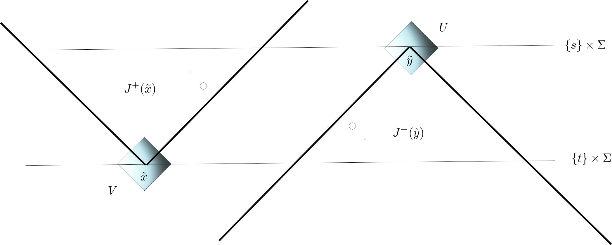
Figure 1: $U\cap J(V)=\emptyset$ and $V\cap J(U)=\emptyset$

Now we show that $K_{G}$ vanishes in $W=V\times U$: Choose smooth functions $\psi$ and $\phi$ with $\operatorname{supp}(\psi)\subset V$ and $\operatorname{supp}(\phi)\subset U$. Then

$$K_{G}(\psi\otimes\phi) =\langle G(\psi),\phi\rangle=\int_{M}G(\psi)\phi\sqrt{g}dx$$

$$=\int_{J(\operatorname{supp}(\psi))\cap\operatorname{supp}(\phi)}G(\psi)\phi\sqrt{g}dx$$

$$=\int_{J(V)\cap U}G(\psi)\phi\sqrt{g}dx=0.$$

∎

Regarding the global regularity of the causal propagator for $C^{1,1}$ globally hyperbolic spacetimes, we find a slightly weaker result compared to the smooth case. Nevertheless, in the ultrastatic setting we show that the same regularity as in the smooth setting holds (Lemma 6.1).

Lemma 5.2.

Let $(M,g)$ be a $C^{1,1}$-globally hyperbolic spacetime.Then $K_{G}\in H_{loc}^{-1-\epsilon}(M\times M)$ for every $\epsilon>0$.

Proof.

We have to show that, given $\psi_{1},\psi_{2}\in{\cal D}(M)$, the Schwartz kernel of the product $\psi_{2}G\psi_{1}$ is in $H^{-1-\varepsilon}(M)$ for every $\varepsilon>0$. Since the proof is local, we may assume (using possibly disconnected coordinate charts) that $\psi_{1}$ and $\psi_{2}$ have their support in the same coordinate neighborhood for $M$. We will therefore work in $\mathbb{R}^{4}$, using the notation $\psi_{1},\psi_{2}$ and $G$ also for the representations in local coordinates. In order to distinguish the standard variables and covariables on $\mathbb{R}^{4}$ from those chosen for $M$ we shall denote them by $\underline{x}$, $\underline{\xi}$, etc.. Moreover, we choose $\psi_{3},\psi_{4}\in{\cal D}(\mathbb{R}^{4})$ supported in the same coordinate chart, satisfying $\psi_{3}\psi_{2}=\psi_{2}$ and $\psi_{4}\psi_{3}=\psi_{3}$. Finally, we denote by $\Lambda^{s}$, $s\in\mathbb{R}$, the pseudodifferential operator of order $s$ with symbol $(1+|\underline{\xi}|^{2})^{s/2}$ on $\mathbb{R}^{4}$.

We have

$$\psi_{2}G\psi_{1}=\Lambda^{1+\varepsilon}\Lambda^{-1-\varepsilon}\psi_{3}\psi_{2}G\psi_{1}=\Lambda^{1+\varepsilon}(\psi_{4}+(1-\psi_{4}))\Lambda^{-1-\varepsilon}\psi_{3}\psi_{2}G\psi_{1}.$$ (5.1)

The operator $\psi_{4}\Lambda^{-1-\varepsilon}\psi_{3}\psi_{2}G\psi_{1}$ maps $H^{1}(\mathbb{R}^{4})$ to $H^{3+\varepsilon}_{comp}(\mathbb{R}^{4})$ and therefore is a Hilbert-Schmidt operator. Hence it has an integral kernel in $L^{2}(\mathbb{R}^{4}\times\mathbb{R}^{4})$. The operator $(1-\psi_{4})\Lambda^{-1-\varepsilon}\psi_{3}$ is obviously smoothing, since $1-\psi_{4}$ and $\psi_{3}$ have disjoint support. Hence it maps $H^{2}(\mathbb{R}^{4})$ to $H^{\infty}(\mathbb{R}^{4})=\bigcap_{s}H^{s}(\mathbb{R}^{4})$. But more is true: In the identity

$$\underline{x}_{j}(1-\psi_{4})\Lambda^{-1-\varepsilon}\psi_{3}=(1-\psi_{4})\Lambda^{-1-\varepsilon}\underline{x}_{j}\psi_{3}+(1-\psi_{4})[\underline{x}_{j},\Lambda^{-1-\varepsilon}]\psi_{3}$$

both operators on the right hand side map $H^{2}(\mathbb{R}^{4})$ to $H^{\infty}(\mathbb{R}^{4})$ (recall that $[\underline{x}_{j},\Lambda^{-1-\varepsilon}]$ has the symbol $D_{\underline{\xi}_{j}}(1+|\underline{\xi}|^{2})^{-1-\varepsilon}$). Iterating this identity we find that $(1+|\underline{x}|^{2N})(1-\psi_{4})\Lambda^{-1-\varepsilon}\psi_{3}\in\mathcal{B}(H^{2}(\mathbb{R}^{4}),H^{\infty}(\mathbb{R}^{4}))$ for every $N\in\mathbb{N}$. Hence $(1-\psi_{4})\Lambda^{-1-\varepsilon}\psi_{3}$ maps $H^{2}(\mathbb{R}^{4})$ to $\mathcal{S}(\mathbb{R}^{4})$.Therefore it also has an integral kernel in $L^{2}(\mathbb{R}^{4}\times\mathbb{R}^{4})$. Denote for the moment the $L^{2}$-integral kernel of $\Lambda^{-1-\varepsilon}\psi_{3}\psi_{2}G\psi_{1}$ by $k_{A}=k_{A}(\underline{x},\underline{y})$. Then the kernel $k=k(\underline{x},\underline{y})$ of $\psi_{2}G\psi_{1}$ is given by

$$\Lambda^{1+\varepsilon}_{(\underline{x})}k_{A}(\underline{x},\underline{y}).$$

Here the notation $\Lambda^{1+\varepsilon}_{(x)}$ indicates that we view $\Lambda^{1+\varepsilon}$ as an operator on $\mathbb{R}^{4}\times\mathbb{R}^{4}$ that acts only with respect to the first copy of $\mathbb{R}^{4}$. In this sense, it is a pseudodifferential operator with symbol in the Hörmander class $S^{1+\varepsilon}_{0,0}$ and thus maps $L^{2}(\mathbb{R}^{4}\times\mathbb{R}^{4})$ to $H^{-1-\varepsilon}(\mathbb{R}^{4}\times\mathbb{R}^{4})$. This shows the assertion.

6 The Ultrastatic Case

In this case we consider a Lorentzian metric $g$ on $M=\mathbb{R}\times\Sigma$ of the form

$$ds^{2}=dt^{2}-h_{ij}(x)dx^{i}dx^{j}$$

where $h_{ij}(x)$ are the components of a time independent Riemannian metric of Hölder regularity $C^{\tau}$ (when $\tau\in\mathbb{N}$ we will consider the Zygmund spaces $C_{*}^{\tau}$, introduced in Definition 3.1).

The Klein-Gordon operator $P$ on $M$ is

$$P\phi=\partial_{tt}\phi-\Delta_{h}\phi+m^{2}\phi$$ (6.1)

with $\Delta_{h}\phi=\frac{1}{\sqrt{h}}\partial_{x^{i}}(h^{ij}\sqrt{h}\partial_{x^{j}}\phi)$ and $m>0$.

The causal propagator $G$ is given by $\displaystyle{-\frac{\sin(A^{\frac{1}{2}}(t-s))}{A^{\frac{1}{2}}}}$ where $A:=-\Delta_{h}+m^{2}$ is self-adjoint on $L^{2}(\Sigma)$, see Appendix 9.2.

Moreover, the spectrum of $A$ is a discrete set of positive eigenvalues which we denote by $\{\lambda_{j}^{2};j=1,2,\ldots\}$, listed according to their (finite) multiplicity. The associated set $\{\phi_{j}\}_{j\in\mathbb{N}}$ of normalized real eigenfunctions is an orthonormal basis of $L^{2}(\Sigma)$, see [32, Theorem 5.8]. For $u,v\in{\mathcal{D}}(M)$ we have $G(v)\in\mathcal{D}^{\prime}(M)$ given by

$$\langle G(v),u\rangle:=$$ (6.2)

$$=\int_{\Sigma}\int_{-\infty}^{\infty}\left(-\frac{\sin(A^{\frac{1}{2}}(t-s))}{A^{\frac{1}{2}}}v\right)(t,x)u(t,x)\sqrt{h(x)}dxdt$$

$$=-\int_{M}\left(\int_{-\infty}^{\infty}\sum_{j}\lambda_{j}^{-1}\sin(\lambda_{j}(t-s))\phi_{j}(x)\int_{\Sigma}\phi_{j}(y)v(s,y)\sqrt{h(y)}dyds\right)u(t,x)\sqrt{h(x)}dxdt,$$

where using that $\langle G(v),u\rangle=\langle K_{G},v\otimes u\rangle$ gives the singular integral kernel representation

$$K_{G}(t,x;s,y)=-\sum_{j}\lambda_{j}^{-1}\sin(\lambda_{j}(t-s))\phi_{j}(x)\phi_{j}(y).$$ (6.3)

6.1 Global Regularity

Now we show in Lemma 6.1 that in ultrastatic spacetimes the global regularity of the causal propagator is the same as in the smooth case

Lemma 6.1.

$K_{G}\in H_{loc}^{-\frac{1}{2}-\epsilon}(M\times M)$ for every $\epsilon>0$.

Proof.

Let $\psi\in\mathcal{D}(M\times M)$. We will show $\psi K_{G}\in H^{-\frac{1}{2}-\epsilon}(M\times M)$. Without loss of generality we take $\psi(t,s,x,y)=\psi_{1}(t)\psi_{2}(s)$ with $\psi_{1},\psi_{2}\in\mathcal{D}(\mathbb{R})$. According to Corollary 4.4

$$\|\psi K_{G}\|^{2}_{H^{-\frac{1}{2}-\epsilon}(M\times M)}$$

$$=\sum_{j=k}\int_{\mathbb{R}^{2}}(\xi_{0}^{2}+\eta_{0}^{2}+\lambda_{j}^{2}+\lambda_{k}^{2})^{-\frac{1}{2}-\epsilon)}\Big{|}{\mathcal{F}_{(t,s)\to(\xi_{0},\eta_{0})}}\Big{(}\frac{\psi(t,s)}{\lambda_{j}}\sin{\lambda_{j}(t-s)}\Big{)}(\xi_{0},\eta_{0})\Big{|}^{2}d\xi_{0}d\eta_{0}.$$

We have by direct computation that

$$\Big{|}{\mathcal{F}_{(t,s)\to(\xi_{0},\eta_{0})}}\Big{(}\frac{\psi(t,s)}{\lambda_{j}}\sin{\lambda_{j}(t-s)}\Big{)}(\xi_{0},\eta_{0})\Big{|}^{2}$$

$$=\frac{1}{\lambda_{j}^{2}}\left|\frac{\hat{\psi}_{1}(\xi_{0}-\lambda_{j})\hat{\psi}_{2}(\eta_{0}+\lambda_{j})-\hat{\psi}_{1}(\xi_{0}+\lambda_{j})\hat{\psi}_{2}(\eta_{0}-\lambda_{j})}{2i}\right|^{2}$$

$$\leq\frac{1}{\lambda_{j}^{2}}\left(\frac{C}{\langle\xi_{0}-\lambda_{j}\rangle^{N}\langle\eta_{0}+\lambda_{j}\rangle^{N}}+\frac{C}{\langle\xi_{0}+\lambda_{j}\rangle^{N}\langle\eta_{0}-\lambda_{j}\rangle^{N}}\right)^{2}$$ (6.4)

for all $N\in\mathbb{N}$ with a suitable constant $C$, since $\psi_{1},\psi_{2}\in\mathcal{D}(M)$. This gives (with constants possibly changing from line to line)

$$\|\psi K_{G}\|_{H^{-\frac{1}{2}-\epsilon}(M\times M)}$$

$$=\sum_{j=k}\int_{\mathbb{R}^{2}}(\xi_{0}^{2}+\eta_{0}^{2}+\lambda_{j}^{2}+\lambda_{k}^{2})^{-\frac{1}{2}-\epsilon}\Big{|}{\mathcal{F}_{(t,s)\to(\xi_{0},\eta_{0})}}\Big{(}\frac{\psi(t,s)}{\lambda_{j}}\sin{\lambda_{j}(t-s)}\Big{)}(\xi_{0},\eta_{0})\Big{|}^{2}d\xi_{0}d\eta_{0}$$

$$\leq\sum_{j=k}\int_{\mathbb{R}^{2}}(\lambda_{j}^{2}+\lambda_{k}^{2})^{-\frac{1}{2}-\epsilon}\frac{1}{\lambda_{j}^{2}}\left(\frac{C}{(\langle\xi_{0}-\lambda_{j}\rangle\langle\eta_{0}+\lambda_{j}\rangle)^{N}}+\frac{C}{(\langle\xi_{0}+\lambda_{j}\rangle\langle\eta_{0}-\lambda_{j}\rangle)^{N}}\right)^{2}d\xi_{0}d\eta_{0}$$

$$\leq C\sum_{j=k}\frac{(\lambda_{j}^{2}+\lambda_{k}^{2})^{-\frac{1}{2}-\epsilon}}{\lambda_{j}^{2}}$$

$$\leq C\sum_{j}\frac{1}{\lambda_{j}^{3+2\epsilon}}.$$

Using Weyl’s law for non-smooth metrics [51, Theorem 1.1] we have the estimate $l^{\frac{2}{3}}\leq C\lambda_{l}^{2}$ for a suitable constant $C$ which gives

$$\|\psi{K}_{G}\|^{2}_{H^{-\frac{1}{2}-\epsilon}(M\times M)} \leq\sum_{l}\frac{C}{\lambda_{l}^{3+\frac{2}{3}\epsilon}}\leq\sum_{l}\frac{C^{\prime}}{l^{1+\epsilon}}<\infty$$

for a suitable constant $C^{\prime}$. ∎

It will be useful to consider the following bidistribution, $K_{A}$ that satisfies $\partial_{t}K_{A}=K_{G}$.

Corollary 6.2.

Let $K_{A}\in\mathcal{D}^{\prime}(M\times M)$ be the bidistribution given by

$$K_{A}(u\otimes v):=\int_{M}\left(\int_{-\infty}^{\infty}\sum_{j}\lambda_{j}^{-2}\cos(\lambda_{j}(t-s))\phi_{j}(x)\int_{\Sigma}\phi_{j}(y)v(s,y)\sqrt{h(y)}dyds\right)u(t,x)\sqrt{h(x)}dxdt,$$

Then,

$$K_{A}\in H_{loc}^{\frac{1}{2}-\epsilon}(M\times M)\text{ for every }\epsilon>0.$$ (6.5)

Proof.

Chose $\psi$ as in the proof of Lemma 6.1. Direct computation shows that

$$\Big{|}{\mathcal{F}_{(t,s)\to(\xi_{0},\eta_{0})}}\Big{(}\frac{\psi(t,s)}{\lambda_{j}^{2}}\cos({\lambda_{j}(t-s)})\Big{)}(\xi_{0},\eta_{0})\Big{|}^{2}$$

$$\leq\frac{1}{\lambda_{j}^{4}}\left(\frac{C}{\langle\xi_{0}-\lambda_{j}\rangle^{N}\langle\eta_{0}+\lambda_{j}\rangle^{N}}+\frac{C}{\langle\xi_{0}+\lambda_{j}\rangle^{N}\langle\eta_{0}-\lambda_{j}\rangle^{N}}\right)^{2}$$

for all $N\in\mathbb{N}$ and a suitable constant $C$. This gives for $s\geq 0$

$$\|\psi K_{A}\|_{H^{s}(M\times M)}$$

$$=\sum_{j=k}\int_{\mathbb{R}^{2}}(|\xi_{0}|^{2}+|\eta_{0}|^{2}+\lambda_{j}^{2}+\lambda_{k}^{2})^{s}\Big{|}{\mathcal{F}_{(t,s)\to(\xi_{0},\eta_{0})}}\Big{(}\frac{\psi(t,s)}{\lambda_{j}^{2}}\cos({\lambda_{j}(t-s)})\Big{)}(\xi_{0},\eta_{0})\Big{|}^{2}d\xi_{0}d\eta_{0}$$

$$\leq C\sum_{j=k}\frac{(\lambda_{j}^{2}+\lambda_{k}^{2})^{s}}{\lambda_{j}^{4}}\leq C^{\prime}\sum_{j}{\lambda_{j}^{2s-4}}$$

for a suitable constant $C^{\prime}$.

According to Weyl’s law for non-smooth metrics [51, Theorem 1.1] we have the estimate $l^{\frac{2}{3}}\leq C\lambda_{l}^{2}$ for a suitable constant $C$. This gives for $s=\frac{1}{2}-\epsilon$, $0<\epsilon\leq\frac{1}{2}$.

$$\|\psi K_{A}\|^{2}_{H^{s}(M\times M)} \leq\sum_{l}\frac{C^{\prime}}{\lambda_{l}^{3+2\epsilon}}\leq\sum_{l}\frac{C^{\prime\prime}}{l^{1+\frac{2}{3}\epsilon}}<\infty$$ (6.6)

for a suitable constant $C^{\prime\prime}$. ∎

6.2 Wavefront Set Estimates

Now we show some some helpful lemmas in order to prove Theorem 6.5 and Theorem 6.7 which are the main results of the section.

First, we establish the microlocal regularity of $K_{G}$ outside the set $\operatorname{Char}(P)\times\operatorname{Char}(P)$.

In the following proofs, we use the distribution $K_{A}$, because a direct application of Theorem 3.3 for $K_{G}$ is not possible, since for $\delta$ close to $1$ the above $\sigma$ cannot take the value $-\frac{1}{2}$.

Lemma 6.3.

For $\tau>2$ and any $\tilde{\epsilon}>0$

$$WF^{-\frac{1}{2}-\tilde{\epsilon}+\tau}(K_{G})\subset\operatorname{Char}(P)\times\operatorname{Char}(P).$$ (6.7)

Proof.

Since $K_{A}$ satisfies $(\partial_{t}+\partial_{s})K_{A}=0$ we conclude that for all $l\in\mathbb{R}$

$$WF^{l}(K_{A})\subset WF(K_{A})\subset\operatorname{Char}(\partial_{t}+\partial_{s})=\{(\tilde{x},\xi^{0},\xi,\tilde{y},\eta^{0},\eta)\in T^{*}(M\times M)\backslash 0;\xi^{0}+\eta^{0}=0\},$$ (6.8)

where the second inclusion follows from the standard theory of pseudodifferential operators.

Now we have $P_{(t,x)}({\bf{x}},D_{\bf{x}})K_{A}=P_{(s,y)}({\bf{x}},D_{\bf{x}})K_{A}=0$. Choose $\epsilon<\tilde{\epsilon}/2$. Since $K_{A}\in H_{loc}^{\frac{1}{2}-\frac{\epsilon}{2}}(M\times M)=H_{loc}^{(\frac{1}{2}-\epsilon)+\frac{\epsilon}{2}}(M\times M)$, an application of Theorem 3.3 with $\sigma=-\frac{3}{2}+\tau-{\epsilon}<\tau-1$ shows that

$$WF^{\frac{1}{2}+\tau-\tilde{\epsilon}}(K_{A})\subset \operatorname{Char}(P_{(t,x)})\cap\operatorname{Char}(P_{(s,y)});$$

here we assume without loss of generality that $\epsilon$ is so small that $-\frac{3}{2}+\tau-{\epsilon}\geq 0$. Eq.(3.10) implies that

$$WF^{\frac{1}{2}-\tilde{\epsilon}+\tau}(K_{A})\subset (\operatorname{Char}(P)\times\operatorname{Char}(P))$$

$$\cup(\{({\bf{x}},{\boldsymbol{\xi}})\in T^{*}(M\times M)\backslash 0,\tilde{\xi}=0,(\tilde{y},\tilde{\eta})\in\operatorname{Char}(P)\}$$

$$\cup\{({\bf{x}},{\boldsymbol{\xi}})\in T^{*}(M\times M)\backslash 0,(\tilde{x},\tilde{\xi})\in\operatorname{Char}(P),\tilde{\eta}=0\}.$$

If $\tilde{\eta}=0$, then $\eta_{0}=0$, and $\xi_{0}=0$ by Eq. (6.8). Since $\operatorname{Char}P=\{(\tilde{x},\tilde{\xi});(\xi_{0})^{2}={\sum_{i=1}^{3}}h^{ij}(x)\xi_{i}\xi_{j}\}$ we then have $\tilde{\xi}=0$. Together with the corresponding argument for the case $\tilde{\xi}=0$ this shows that

$$WF^{\frac{1}{2}-\tilde{\epsilon}+\tau}(K_{A})\subset\operatorname{Char}(P)\times\operatorname{Char}(P);$$ (6.9)

otherwise $0\in T^{*}(M\times M)$ will be in $WF^{\frac{1}{2}-\tilde{\epsilon}+\tau}(K_{A})$.

Since $WF^{-\frac{1}{2}-\tilde{\epsilon}+\tau}(\partial_{t}K_{A})\subset WF^{\frac{1}{2}-\tilde{\epsilon}+\tau}(K_{A})$ by [27, Proposition B.3], we have

$$WF^{-\frac{1}{2}-\tilde{\epsilon}+\tau}(K_{G})=WF^{-\frac{1}{2}-\tilde{\epsilon}+\tau}(\partial_{t}K_{A})\subset WF^{\frac{1}{2}-\tilde{\epsilon}+\tau}(K_{A})\subset(\operatorname{Char}(P)\times\operatorname{Char}(P)).$$

∎

Now we establish that points above the diagonal are of a specific form.

Lemma 6.4.

If $(\tilde{x},\tilde{\xi},\tilde{x},\tilde{\eta})\in WF^{-\frac{3}{2}-\tilde{\epsilon}+\tau}(K_{G})$ for $\tau>2$ and some $\tilde{\epsilon}>0$, then $\tilde{\eta}=-\tilde{\xi}$.

Proof.

Suppose $\tilde{\eta}$ and $\tilde{\xi}$ are linearly independent, i.e., $\tilde{\eta}\neq\lambda\tilde{\xi}$ for $\lambda\in\mathbb{R}$. By Eq.(6.9) $(\tilde{x},\tilde{\xi},\tilde{x},\tilde{\eta})\in\operatorname{Char}(P)\times\operatorname{Char}(P)$. Now we choose a Cauchy hypersurface $\Sigma_{t_{0}}=\{t_{0}\}\times\Sigma$ such that the null geodesic with initial data $(\tilde{x},\tilde{\xi})$ and the null geodesic with initial data $(\tilde{x},\tilde{\eta})$ intersect it. These points of intersections are unique by global hyperbolicity. Moreover, using the condition $\tilde{\eta}\neq\lambda\tilde{\xi}$, we can choose $\Sigma_{t_{0}}$ such that these points are distinct. We denote these points by $(t_{0},x_{0}),(t_{0},y_{0})$. Furthermore, they are not causally related.

Notice that $K_{A}$ satisfies $P_{(t,x)}K_{A}=0$, $P^{b}_{(t,x)}K_{A}\in H^{-\frac{3}{2}-\epsilon+\tau}(M\times M)$ by taking into account Remark 3.4 for a choice of $\delta$ close to $1$. This allows us to choose $s=-\frac{3}{2}-\epsilon+\tau$, which is in the range $0<s<\tau-1$ in Theorem 3.5. This propagation of singularities result applied to the distribution $K_{A}$ and the operator $P_{(t,x)}$ guarantees that if $(\tilde{x},\tilde{\xi},\tilde{x},\tilde{\eta})\in WF^{-\frac{3}{2}-\epsilon+\tau}(K_{G})\subset WF^{-\frac{1}{2}-\epsilon+\tau}(K_{A})$ then the full null bicharacteristic is contained in the wavefront set i.e. $(\gamma(\tilde{x},\tilde{\xi}),(\tilde{x},\tilde{\eta}))\in{WF^{-\frac{1}{2}-\epsilon+\tau}(K_{A})}$, where $\gamma(\tilde{x},\tilde{\xi})$ is the null bicharacteristic with initial data $(\tilde{x},\tilde{\xi})$. Similarly, using the operator $P_{(s,y)}$, we obtain $(\gamma(\tilde{x},\tilde{\xi}),\gamma(\tilde{x},\tilde{\eta}))\in{WF^{-\frac{1}{2}-\epsilon+\tau}(K_{A})}$ where $\gamma(\tilde{x},\tilde{\eta})$ is the null bicharacteristic with initial data $(\tilde{x},\tilde{\eta})$.

Now we show that this set of points is contained in ${WF^{-\frac{1}{2}-\epsilon+\tau}(K_{G})}$.

By Theorem 6.1.1’ from [14] we have

$${WF^{-\frac{1}{2}-\epsilon+\tau}(K_{A})\backslash WF^{-\frac{1}{2}-\epsilon+\tau}(K_{G})=WF^{-\frac{1}{2}-\epsilon+\tau}(K_{A})\backslash WF^{-\frac{1}{2}-\epsilon+\tau}(\partial_{t}K_{A})}\subset\operatorname{Char}(\partial_{t}).$$ (6.10)

However, using Eq.(6.9) and that $(\partial_{t}+\partial_{s})K_{A}=0$, we have the inclusion

$${WF^{-\frac{1}{2}-\epsilon+\tau}(K_{A})\subset WF^{\frac{1}{2}-\epsilon+\tau}(K_{A})}\subset(\operatorname{Char}(P)\times\operatorname{Char}(P))\cap\operatorname{Char}(\partial_{t}+\partial_{s})$$ (6.11)

Since $(\operatorname{Char}(P)\times\operatorname{Char}(P))\cap\operatorname{Char}(\partial_{t}+\partial_{s})\cap\operatorname{Char}(\partial_{t})=\emptyset$, taking the intersection between Eq.(6.10) and Eq.(6.11), we obtain that the left hand side of Eq.(6.10) must be empty. Therefore,

$${WF^{-\frac{1}{2}-\epsilon+\tau}(K_{A})\subset WF^{-\frac{1}{2}-\epsilon+\tau}(K_{G}).}$$ (6.12)

Hence, $(\gamma(\tilde{x},\tilde{\xi}),\gamma(\tilde{x},\tilde{\eta}))\in{WF^{-\frac{1}{2}-\epsilon+\tau}}(K_{G})$.

In particular $(t_{0},x_{0},t_{0},y_{0})\in\Pi({WF^{-\frac{1}{2}-\epsilon+\tau}}(K_{G}))$, where $\Pi$ is the projection from $T^{*}(M\times M)$ to $M\times M$. However, this is a contradiction to Proposition 5.1, since $(t_{0},x_{0},t_{0},y_{0})\notin\operatorname{supp}(K_{G})$. Therefore, $\tilde{\eta}=\lambda\tilde{\xi}$. Using Eq.(6.8) we have $\xi^{0}=-\eta^{0}$ which gives $\lambda=-1$ i.e. $\tilde{\eta}=-\tilde{\xi}$. ∎

Now we state one of the main results:

Theorem 6.5.

Let $(M,g)$ be a $C^{\tau}$ ultrastatic spacetime with $\tau>2$ and $K_{G}$ the causal propagator. Then $WF^{\prime-\frac{3}{2}-{\epsilon}+\tau}(K_{G})\subset C$ for every ${\epsilon}>0$ and $C$ as in Eq.(1.1).

Proof.

Let $(\tilde{x},\tilde{\xi},\tilde{y},-\tilde{\eta})\in WF^{-\frac{3}{2}-{\epsilon}+\tau}(K_{G})$. The propagation of singularities result (Theorem 3.5) implies that $(\gamma(\tilde{x},\tilde{\xi}),\gamma(\tilde{y},-\tilde{\eta}))\in{WF^{-\frac{1}{2}-\epsilon+\tau}}(K_{A})$, where $\gamma(\tilde{x},\tilde{\xi})$ is the null bicharacteristic with initial data $(\tilde{x},\tilde{\xi})$ and $\gamma(\tilde{y},-\tilde{\eta})$ is the null bicharacteristic with initial data $(\tilde{y},-\tilde{\eta})$. Arguing as in the proof of Lemma 6.4 by Eq.(6.11), Lemma 6.3, the fact that $(\partial_{t}+\partial_{s})K_{G}=0$ and the inclusion $WF^{s}(K_{A})\subset WF^{s-1}(K_{G})\cup\operatorname{Char}(\partial_{t})$ for all $s\in\mathbb{R}$, we have $(\gamma(\tilde{x},\tilde{\xi}),\gamma(\tilde{y},-\tilde{\eta}))\in{WF^{-\frac{3}{2}-\epsilon+\tau}}(K_{G})$.

Now we choose a Cauchy surface $\Sigma_{t_{1}}=\{t_{1}\}\times\Sigma$ and suppose that $(t_{1},x_{1},\tilde{\xi}_{1},t_{1},x_{2},\tilde{\xi}_{2})\in(\gamma(\tilde{x},\tilde{\xi}),\gamma(\tilde{y},-\tilde{\eta}))\cap(\Sigma_{t_{1}}^{2})$. By Lemmas 5.1 and 6.4, $(t_{1},x_{1},\tilde{\xi}_{1}),(t_{1},x_{2},\tilde{\xi}_{2})\in\operatorname{Char}(P)$, $x_{1}=x_{2}$, and $\tilde{\xi}_{2}=-\tilde{\xi}_{1}$.

Next we define a curve $\tilde{\gamma}:(-\infty,\infty)\rightarrow M$ as follows. First, we shift the parametrization $\lambda$ in the definition of the null bicharacteristics so that

$$\gamma(\tilde{x},\tilde{\xi})(t_{1})=(t_{1},x_{1},\tilde{\xi}_{1})\quad\gamma(\tilde{y},-\tilde{\eta})(t_{1})=(t_{1},x_{1},-\tilde{\xi}_{1}).$$

Then, we denote by $\Pi:T^{*}M\to M$ the canonical projection and define two curves in $M$ by

$$\gamma_{1}(\lambda):=\Pi(\gamma(\tilde{x},\tilde{\xi})(\lambda))\quad\gamma_{2}(\lambda):=\Pi(\gamma(\tilde{y},-\tilde{\eta})(\lambda)).$$

Notice that we have ${\gamma_{1}}(t_{1})=(t_{1},x_{1}),\dot{\gamma_{1}}(t_{1})=g^{-1}(\tilde{\xi}_{1},\cdot)$ and ${\gamma_{2}}(t_{1})=(t_{1},x_{1}),\dot{\gamma_{2}}({t_{1}})=g^{-1}(-\tilde{\xi}_{1},\cdot)$. Moreover, we can assume that $\tilde{x}=\gamma_{1}(a)$ and $\tilde{y}=\gamma_{2}(b)$ for suitable $a,b\in\mathbb{R}$ with $a<t_{1}<b$.

Finally, let

$$\tilde{\gamma}(\lambda)=\begin{cases}\gamma_{1}(\lambda)&\lambda\in(-\infty,t_{1}]\\ -\gamma_{2}(\lambda)&\lambda\in(t_{1},\infty)\end{cases}$$ (6.13)

where $-\gamma_{2}$ denotes the curve with opposite orientation.

Then $\tilde{\gamma}(a)=\tilde{x}$, $\tilde{\gamma}(b)=\tilde{y}$; moreover $g(\cdot,{\dot{\tilde{\gamma}}})|_{T_{\tilde{x}}M}=\tilde{\xi}$, $g(\cdot,{\dot{\tilde{\gamma}}})|_{T_{\tilde{y}}M}=\tilde{\eta}$ and therefore, $\tilde{\gamma}$ is a null geodesic between $\tilde{x}$ and $\tilde{y}$ with cotangent vectors $\tilde{\xi}$ at $\tilde{x}$ and $\tilde{\eta}$ at $\tilde{y}$, i.e. $(\tilde{x},\tilde{\xi},\tilde{y},-\tilde{\eta})\in C^{\prime}:=\{(\tilde{x},\tilde{\xi},\tilde{y},-\tilde{\eta});(\tilde{x},\xi;\tilde{y},\tilde{\eta})\in C\}$, see Figure 2.

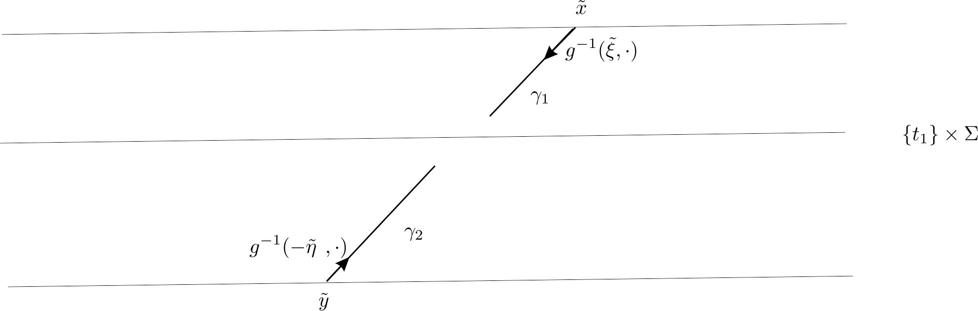
Figure 2: $\gamma_{1}$ is a null geodesic that satisfies $\gamma(a)=\tilde{x},\dot{\gamma}_{1}(a)=g^{-1}(\xi,\dot{)}$ and $\gamma_{2}$ is a null geodesic that satisfies $\gamma(b)=\tilde{y},\dot{\gamma}_{2}(b)=g^{-1}(-\eta,\cdot)$

This shows

$${WF^{-\frac{3}{2}-\epsilon+\tau}}(K_{G})\subset C^{\prime}$$ (6.14)

Using the definition of $WF^{l^{\prime}}(u):=\{(\tilde{x},\tilde{\eta};\tilde{y},-\tilde{\eta})\in T^{*}(M\times M);(\tilde{x},\tilde{\xi};\tilde{y},\tilde{\eta})\in WF^{l}(u)\}$ gives the result.

∎

For the analysis of adiabatic states it is enough to work with the inclusion shown above. However, in the smooth case we have an equality of sets. In Theorem 6.7, we show that this equality holds under stronger regularity assumptions on the metric.

First we show the following lemma

Lemma 6.6.

Let $(\tilde{x},\tilde{\xi})\in\operatorname{Char}(P)$ with $P$ as in Eq. (6.1).Then $(\tilde{x},\tilde{x},\tilde{\xi},-\tilde{\xi})\in WF^{\frac{3}{2}+{\epsilon}}(K_{G})$ for all ${\epsilon}>0.$

Proof.

Since $WF^{s_{1}}\subset WF^{s_{2}}$ for $s_{1}\leq s_{2}$, it is enough to show the result for small $\epsilon$. Let $Q:=\mathbb{R}\times\Sigma^{2}$. We define the embedding $f:Q\rightarrow M\times M$ by $f(s,x,y)=(s,x,s,y)$. The set of normals of the map $f$ is

$$N_{f} =\{(f(s,x,y),\tilde{\xi},\tilde{\eta})\in T^{*}(M\times M);^{t}f^{\prime}(s,x,y)(\tilde{\xi},\tilde{\eta})=0\}$$

$$=\{(s,x,s,y,\xi^{0},0,-\xi^{0},0)\in T^{*}(M\times M)\},$$

where ${}^{t}f^{\prime}$ is the transpose of the differential of $f$. In particular, $N_{f}\cap(\operatorname{Char}P\times\operatorname{Char}P)=\emptyset$. By Lemma 6.3,

$$WF^{\frac{3}{2}+{\epsilon}}(K_{G})\cap N_{f}=\emptyset$$

and therefore

$$WF^{\frac{1}{2}+\epsilon}(\partial_{t}K_{G})\cap N_{f}\subset WF^{\frac{3}{2}+{\epsilon}}(K_{G})\cap N_{f}=\emptyset$$

for suitably small $\epsilon>0$. Therefore Proposition B.7 from [27] implies that the restriction of $\partial_{t}K_{G}$ to ${Q}$ is defined and satisfies

$$WF^{\epsilon}(\partial_{t}K_{G}|_{Q}) \subset f^{*}(WF^{{\frac{1}{2}+\epsilon}}(\partial_{t}K_{G}))$$ (6.15)

$$=\{(s,x,y,^{t}f^{\prime}(\tilde{\xi},\tilde{\eta}))\in T^{*}Q;(f(s,x,y),\tilde{\xi},\tilde{\eta})\in{WF^{\frac{1}{2}+\epsilon}}(\partial_{t}K_{G})\}$$

As a distribution, $\partial_{t}{K_{G}}|_{Q}$ is given by

$$\partial_{t}K_{G}|_{Q}(s,x,y)=-\sum_{j}\phi_{j}(x)\phi_{j}(y),$$

i.e., it acts on the non-smooth density $\psi_{1}(s)\psi_{2}(x)\psi_{3}(y)\sqrt{h}(x)\sqrt{h}(y)dxdy$, by

$$\langle\partial_{t}K_{G}|_{Q},\psi_{1}\psi_{2}\psi_{3}\rangle=-\int_{-\infty}^{\infty}\psi_{1}(p)dp\int_{\Sigma}\psi_{2}(w)\psi_{3}(w)\sqrt{h(w)}dw.$$ (6.16)

Therefore its Fourier transform is given by

$$({\cal{F}}(\partial_{t}K_{G}|_{Q}))({\chi},\xi,\eta)=\delta_{0}(\chi)\otimes\int_{\Sigma}e^{-iw(\xi+\eta)}\sqrt{h(w)}dw.$$ (6.17)

Moreover, we have $(\partial_{t}K_{G}|_{Q}-1\otimes\delta(x-y))(\psi)=0$ for all smooth densities on $\mathbb{R}\times\Sigma\times\Sigma$. Therefore $\partial_{t}K_{G}|_{Q}=1\otimes\delta(x-y)$ as elements of ${\cal{D}}^{\prime}(\mathbb{R}\times\Sigma\times\Sigma)$. This implies

$$WF^{s}(\partial_{t}K_{G}|_{Q})=\begin{cases}\emptyset,s<-\frac{3}{2}\\ (s,x,x,0,\xi,-\xi)\text{ for all }\xi\in T^{*}_{x}\Sigma,s\geq-\frac{3}{2}.\end{cases}$$

Using Eq. (6.15) we find that there exists $\xi_{0}$ such that $(s,x,s,x,\xi^{0},\xi,-\xi^{0},-\xi)\in WF^{\frac{1}{2}+\epsilon}(\partial_{t}K_{G})$ for each $\xi\in T^{*}\Sigma$.

According to Proposition B.3 from [27]

$$WF^{\frac{1}{2}+\epsilon}(\partial_{t}K_{G})\subset WF^{\frac{3}{2}+\epsilon}(K_{G}).$$ (6.18)

Since the wavefront set is contained in $\operatorname{Char}(P)\times\operatorname{Char}(P)$ we obtain from Lemma 6.3 $(s,x,s,x,\xi^{0},\xi,-\xi^{0},-\xi)\in\operatorname{Char}(P)\times\operatorname{Char}(P)$ with $\xi_{0}^{2}=h^{ij}\xi_{i}\xi_{j}$. Without loss of generality we choose a sign for $\xi_{0}$ i.e. $\xi_{0}:=\sqrt{h^{ij}\xi_{i}\xi_{j}}$.

Now we show that if $(s,x,s,x,\xi^{0},\xi,-\xi^{0},-\xi)\in WF^{\frac{3}{2}+\epsilon}(K_{G})$ then $(s,x,s,x,-\xi^{0},-\xi,\xi^{0},\xi)\in WF^{\frac{3}{2}+\epsilon}(K_{G})$. The diffeomorphism $f_{1}(t,x,s,y)=(s,y,t,x)$ has the set of normals $N_{f_{1}}=\{(s,y,t,x,0,0,0,0)\in T^{*}(M\times M)\}$ which has empty intersection with $WF(K_{G})$. Then [22, Theorem 8.2.3] and the invariance of the Sobolev wavefront set implies that

$$WF^{\frac{3}{2}+\epsilon}(f_{1}^{*}K_{G})=f_{1}^{*}WF^{\frac{3}{2}+\epsilon}(K_{G}).$$ (6.19)

Moreover $f_{1}^{*}K_{G}=-K_{G}$ which gives

$$WF^{\frac{3}{2}+\epsilon}(K_{G})=f_{1}^{*}WF^{\frac{3}{2}+\epsilon}(K_{G}).$$ (6.20)

Now since $(s,x,s,x,\xi^{0},\xi,-\xi^{0},-\xi)\in WF^{\frac{3}{2}+\epsilon}(K_{G})$ then we have $(s,x,s,x,-\xi^{0},-\xi,\xi^{0},\xi)\in WF^{\frac{3}{2}+\epsilon}(K_{G})$ by Eq.(6.22).

Notice that we also have to show that $(s,x,s,x,-\xi^{0},\xi,\xi^{0},-\xi)$ and $(s,x,s,x,\xi^{0},-\xi,-\xi^{0},\xi)$ are in $WF^{\frac{3}{2}+\epsilon}(K_{G})$.

In this case we use the diffeomorphism $f_{2}(t,x,s,y)=(s,x,t,y)$ that has the set of normals $N_{f_{2}}=\{(s,x,t,y,0,0,0,0)\in T^{*}(M\times M)\}$ which has empty intersection with $WF(K_{G})$. Then [22, Theorem 8.2.3] and the invariance of the Sobolev wavefront set implies that

$$WF^{\frac{3}{2}+\epsilon}(f_{2}^{*}K_{G})=f_{2}^{*}WF^{\frac{3}{2}+\epsilon}(K_{G}).$$ (6.21)

Moreover $f_{2}^{*}K_{G}=-K_{G}$ which gives

$$WF^{\frac{3}{2}+\epsilon}(K_{G})=f_{2}^{*}WF^{\frac{3}{2}+\epsilon}(K_{G}).$$ (6.22)

Now since $(s,x,s,x,\xi^{0},\xi,-\xi^{0},-\xi)\in WF^{\frac{3}{2}+\epsilon}(K_{G})$ then we have $(s,x,s,x,-\xi^{0},\xi,\xi^{0},-\xi)\in WF^{\frac{3}{2}+\epsilon}(K_{G})$ by Eq.(6.22). Using $f_{1}$ we obtain $(s,x,s,x,\xi^{0},-\xi,-\xi^{0},\xi)\in WF^{\frac{3}{2}+\epsilon}(K_{G})$. This gives the desired result.

∎

Now we show the equality of sets as in the smooth case.

Theorem 6.7.

Let $(M,g)$ be a $C^{\tau}$ ultrastatic spacetime with $\tau>3$ and $K_{G}$ the causal propagator. Then $C\subset WF^{\prime-\frac{3}{2}+\tau-\tilde{\epsilon}}(K_{G})$ for all $\tilde{\epsilon}<\tau-3$ and $C$ as in Eq.(1.1). In particular, we have $C\subset WF^{\prime s}(K_{G})$ for all $s>\frac{3}{2}$.

Proof.

Under the additional regularity assumption and arguing locally as in Theorem 3.3, we have $P^{b}_{(t,x)}K_{A},P^{b}_{(s,y)}K_{A}\in H^{\frac{3}{2}+\tilde{\epsilon}}(M\times M)$ and therefore for $(\tilde{x},\tilde{\xi},\tilde{y},\tilde{\eta})\in WF^{\frac{3}{2}+\tilde{\epsilon}}(K_{G})\subset WF^{\frac{5}{2}+\tilde{\epsilon}}(K_{A})$ we can choose $s=\frac{3}{2}+\tilde{\epsilon}$ in Theorem 3.5.

Now if $({\bf{x}},{\boldsymbol{\xi}})=(\tilde{x},\tilde{\xi},\tilde{y},-\tilde{\eta})\in C^{\prime}$ then there is a null geodesic $\gamma$ such that $\gamma(t_{1})=\tilde{x},\gamma(t_{2})=\tilde{y}$ and $g(\cdot,{\dot{\gamma}})|_{T_{\tilde{x}}M}=\tilde{\xi},g(\cdot,{\dot{\gamma}})|_{T_{\tilde{y}}M}=\tilde{\eta}$. Now, $(\tilde{x},\tilde{\xi},\tilde{x},-\tilde{\xi})\in C^{\prime}$ and by Lemma 6.6 $(\tilde{x},\tilde{\xi},\tilde{x},-\tilde{\xi})\in WF^{\frac{3}{2}+\epsilon}(K_{G})$ for $\epsilon>0$ which implies for $\tilde{\epsilon}<\tau-3$ that $(\tilde{x},\tilde{\xi},\tilde{x},-\tilde{\xi})\in WF^{-\frac{3}{2}+\tau-\tilde{\epsilon}}(K_{G})\subset WF^{-\frac{1}{2}+\tau-\tilde{\epsilon}}(K_{A})$. Applying Theorem 3.5 to $P_{(t,x)}K_{A},P_{(s,y)}K_{A}$ with the $s$ described above we have $(\gamma(\tilde{x},\tilde{\xi}),\gamma(\tilde{x},-\tilde{\xi}))\in WF^{-\frac{1}{2}+\tau-\tilde{\epsilon}}(K_{A})$. Using the same argument as in Theorem 6.5 this implies $(\tilde{x},\tilde{\xi},\tilde{y},-\tilde{\eta})=({\bf{x}},{\boldsymbol{\xi}})\in WF^{-\frac{3}{2}+\tau-\tilde{\epsilon}}(K_{G})$. ∎

Remark 6.8.

The combination of Theorem 6.5 with Theorem 6.7 gives

$$WF^{\prime-\frac{3}{2}+\tau-\tilde{\epsilon}}(K_{G})=C$$

for $\tau>3$ and $\tilde{\epsilon}<\tau-3$.

6.3 The $C^{1,1}$ Case

The following theorem states the result for the case of $C^{1,1}$ regularity.

Theorem 6.9.

Let $(M,g)$ be a $C^{1,1}$ ultrastatic spacetime and $K_{G}$ the causal propagator. Then $WF^{\prime\frac{1}{2}-\tilde{\epsilon}}(K_{G})\subset C$ for all $\tilde{\epsilon}>0$.

Proof of Theorem 6.9. In order to show the theorem we will state how different results of the paper change under this regularity.

From the comment above Theorem 3.5 we know that Theorem 3.5 still holds.

Also, notice that a $C^{1,1}$ metric guarantees the existence and uniqueness of the Hamiltonian flow which is critical for the proof. Theorem 3.3 holds even for $\tau>1$.

Lemma 5.1 requires no modification, since the results on global hyperbolicity still hold for this regularity [41, Corollary 3.4]. The hypothesis in [51, Theorem 1.1] is the requirement that the coefficients of the principal part have one derivative that is Lipschitz which is clearly satisfied in the $C^{1,1}$ case. Hence Lemma 6.1 holds.

For Lemma 6.4 and Theorem 6.5 the only thing to notice is that in this case $P_{(t,x)}^{b}K_{A},P_{(s,y)}^{b}K_{A}\in H^{\frac{1}{2}-\tilde{\epsilon}(M\times M)}$ (arguing locally as in Theroem 3.3) and therefore we can apply Theorem 3.5 for $s=\frac{1}{2}-\tilde{\epsilon}$. In this section we have applied the version of Theorem 3.5 after [49, Proposition 11.4]. ∎

7 The Stationary Case

In this section we show the results of the previous sections hold for the stationary case if one allows higher regularity of the spacetime metric. Moreover, in this section, we will generalise the discussion to include operators of the form $P_{V}:=\square_{g}+V(t,x)$

A stationary spacetime is given by a Riemannian manifold $h$, a function $N(x)>0$ and a $1$-form $\beta_{i}(x)dx^{i}$ such that the spacetime metric $(M,g)$, where $M=\mathbb{R}\times\Sigma$, is given by

$$ds^{2}=N^{2}(x)dt^{2}-(dx^{i}+\beta^{i}(x)dt)h_{ij}(x)(dx^{j}+\beta^{j}(x)dt)$$ (7.1)

and $N^{2}(x)>\beta_{i}(x)h^{ij}(x)\beta_{j}(x)$. We will assume the regularity of $h$, $\beta_{i}$ and $N$ is $C^{\tau}$.

In this section we will prove the following two results.

Theorem 7.1.

Let $(M,g)$ be a $C^{\tau}$ stationary spacetime with $\tau>2$ and $K_{G}$ the causal propagator of $\square_{g}$. Then $WF^{\prime-2-{\epsilon}+\tau}(K_{G})\subset C$ for every ${\epsilon}>0$ and $C$ as in Eq.(1.1).

Theorem 7.2.

Let $(M,{g})$ be a $C^{\tau}$ stationary spacetime with $\tau>2$ and $K_{G_{V}}$ the causal propagator of the operator $P_{V}:=\square_{g}+V(t,x)$ where $V(t,x)\in C^{1}_{b}$. Then $WF^{\prime-{\epsilon}}(K_{G_{V}})\subset C$ for every ${\epsilon}>0$ and $C$ as in Eq.(1.1).

∎

7.1 Proof of Theorem 7.1

An important difference compared to the ultrastatic case is that we cannot take recourse to the auxiliary distribution $K_{A}$ in the stationary case. This distribution was introduced because $K_{G}$ is not in the domain of $P_{(t,x)}^{b}$ . However, using the divergence structure of the operator one can find a decomposition such that the non-smooth operator has a larger domain. We expand Remark 3.6 and also focus now on the operator $\square_{g}$ instead of $\square_{g}+m^{2}$. The proofs are very similar to the ones in the ultrastatic case but we state them for convenience of the reader.

Let $u$ satisfy $P_{(t,x)}({\bf{x}},D_{\bf{x}})u=0$ with $u\in H_{loc}^{1+s-\tau\delta}(M\times M)$. Then also

$$\partial_{\nu}\left(\sqrt{|g|}g^{\mu\nu}\partial_{\mu}u\right)=0.$$

Using the decomposition $\sqrt{|g|}g^{\mu\nu}\partial_{\mu}=(\sqrt{|g|}g^{\mu\nu}\partial_{\mu})^{\#}+(\sqrt{|g|}g^{\mu\nu}\partial_{\mu})^{b}$ we obtain

$$P_{(t,x)}({\bf{x}},D_{\bf{x}})v=\frac{1}{\sqrt{|g|}}\partial_{\mu}\left((\sqrt{|g|}g^{\mu\nu}\partial_{\mu})^{\#}v+(\sqrt{|g|}g^{\mu\nu}\partial_{\mu})^{b}v\right),$$ (7.2)

where $\partial_{\nu}(\sqrt{|g|}g^{\mu\nu}\partial_{\mu})^{b}:H^{s+1-\tau\delta}_{comp}(M\times M)\rightarrow H^{s-1}(M\times M)$ for $-(1-\delta)\tau<s<\tau$.

In particular since $K_{G}\in H_{loc}^{-1-\epsilon}(M\times M)$, arguing locally as in Theorem 3.3, is in the domain of $\partial_{\nu}(\sqrt{|g|}g^{\mu\nu}\partial_{\mu})^{b}$ for $\tau>2$ choosing $s=0$.

We state the behaviour outside the characteristic in this setting.

Lemma 7.3.

For $\tau>2$ and any $\tilde{\epsilon}>0$

$$WF^{-1-\tilde{\epsilon}+\tau}(K_{G})\subset\operatorname{Char}(P)\times\operatorname{Char}(P).$$ (7.3)

Proof.

Notice that since $P_{(t,x)}({\bf{x}},D_{\bf{x}})K_{G}=0$ we have

$$\partial_{\nu}(\sqrt{|g|}g^{\mu\nu}\partial_{\mu})^{\#}K_{G}=-\partial_{\nu}(\sqrt{|g|}g^{\mu\nu}\partial_{\mu})^{b}K_{G},$$ (7.4)

where $-\partial_{\nu}(\sqrt{|g|}g^{\mu\nu}\partial_{\mu})^{b}K_{G}\in H^{-3-\epsilon+\tau\delta}(M\times M)$.

Now if $({\bf{x}}_{0},{\boldsymbol{\xi}}_{0})\not\in\operatorname{Char}(P_{(t,x)})$ and $0<\sqrt{|g(\tilde{x})|}$, then $|g^{\mu\nu}\sqrt{|g(\tilde{x})|}\xi_{\mu}\xi_{\nu}|\geq C|{\boldsymbol{\xi}}|^{2}$ for large $|{\boldsymbol{\xi}}|$ in a conic neighbourhood of $({\bf{x}}_{0},{\boldsymbol{\xi}}_{0})$. This gives $({\bf{x}}_{0},{\boldsymbol{\xi}}_{0})\not\in\operatorname{Char}(\partial_{\nu}(\sqrt{|g|}g^{\mu\nu}\partial_{\mu})^{\#})$. Therefore we can use a microlocal parametrix $\tilde{q}\in S^{-2}_{1,\delta}$ such that

$$\tilde{q}\partial_{\nu}(\sqrt{|g|}g^{\mu\nu}\partial_{\mu})^{\#}K_{G}=K_{G}+r({\bf{x}},D)K_{G}$$ (7.5)

and $({\bf{x}}_{0},{\boldsymbol{\xi}}_{0})\not\in WF(r({\bf{x}},D)K_{G})$. Moreover, using Eq.(7.4) we have $\tilde{q}\partial_{\nu}(\sqrt{|g|}g^{\mu\nu}\partial_{\mu})^{\#}K_{G}=-\tilde{q}\partial_{\nu}(\sqrt{|g|}g^{\mu\nu}\partial_{\mu})^{b}K_{G}\in H^{-1-\epsilon+\tau\delta}(M\times M)$. Since $0\leq\delta<1$ can be chosen arbitrarily, $({\bf{x}}_{0},{\boldsymbol{\xi}}_{0})\not\in WF^{-1-\tilde{\epsilon}+\tau}(K_{G})$ for any $\tilde{\epsilon}>0$ i.e. $WF^{-1-\tilde{\epsilon}+\tau}(K_{G})\subset\operatorname{Char}(P_{(t,x)})$.

Similarly we have $P_{(s,y)}({\bf{x}},D_{\bf{x}})K_{G}=0$. Therefore,

$$WF^{-1+\tau-\tilde{\epsilon}}(K_{G})\subset \operatorname{Char}(P_{(t,x)})\cap\operatorname{Char}(P_{(s,y)}).$$ (7.6)

In order to conclude the proof we use the important fact that in stationary spacetimes $K_{G}$ satisfies $(\partial_{t}+\partial_{s})K_{G}=0$ ([13, Remark 5.7]) therefore we can conclude that for all $l\in\mathbb{R}$

$$WF^{l}(K_{G})\subset WF(K_{G})\subset\operatorname{Char}(\partial_{t}+\partial_{s})=\{(\tilde{x},\xi^{0},\xi,\tilde{y},\eta^{0},\eta)\in T^{*}(M\times M)\backslash 0;\xi^{0}+\eta^{0}=0\},$$ (7.7)

where the second inclusion follows from the standard theory of pseudodifferential operators.

Finally, Eq.(7.6) and Eq. (7.7) imply that

$$WF^{-1-\tilde{\epsilon}+\tau}(K_{G})\subset(\operatorname{Char}(P)\times\operatorname{Char}(P)).$$

∎

The proof of Lemma 6.4 can be modified in a similar way. The main tool for the proof is the propagation of singularities result, which is already in the setting described above. However, compared to the ultrastatic spacetime we have $K_{G}\in H^{-1-\epsilon}$ so $\partial_{\nu}(\sqrt{|g|}g^{\mu\nu}\partial_{\mu})^{b}K_{G}\in H^{-3-\epsilon+\tau\delta}$ and therefore if $(\tilde{x},\tilde{\xi},\tilde{y},-\tilde{\eta})\in WF^{-2-{\epsilon}+\tau}(K_{G})$ then $(\gamma(\tilde{x},\tilde{\xi}),\gamma(\tilde{y},-\tilde{\eta}))\in{WF^{-2-\epsilon+\tau}}(K_{G})$.

Finally, using the above observations and a similar argument to the one used in the proof of Theorem 6.5 gives the result.

7.2 Proof of Theorem 7.2

Proof.

We define $P_{\tilde{V}}:=\square_{g}+\chi V$ where $\chi$ is a compactly supported smooth function equal to one in a time slab $\Omega:=(-t,t)\times\Sigma$

Now, let $f\in L^{2}_{comp}(M)$; let $G^{+}$ be the advanced Green operator of $\square_{g}$ and $G^{+}_{\tilde{V}}$ the advanced Green operator of $P_{\tilde{V}}$. Then $G^{+}(f)=:\phi\in H^{1}_{loc}(M)$ satisfies $\square_{g}\phi=f$ with $\operatorname{supp}(\phi)\subset J^{+}(\operatorname{supp}(f))$ and $G^{+}_{\tilde{V}}(f)=:\psi\in H^{1}_{loc}(M)$ satisfies $\square_{g}\psi+\chi V\psi=f$ with $\operatorname{supp}(\psi)\subset J^{+}(\operatorname{supp}(f))$.

Therefore $P_{\tilde{V}}(\phi-\psi)=\chi V\phi$. Defining $\Psi:=\phi-\psi$ and $\tilde{f}:=\chi V\phi\in H^{1}_{comp}(M)$ we have that $P_{\tilde{V}}\Psi=\tilde{f}$. Noticing that there exists a Cauchy surface such that $\Psi|_{\Sigma_{t}}=n^{\mu}\nabla_{\mu}\Psi|_{\Sigma}=0$ we have by [24, Theorem 4.7] that $\Psi\in H^{2}_{loc}(M)$. This implies

$$G^{+}-G^{+}_{\tilde{V}}:L^{2}_{comp}(M)\rightarrow H^{2}_{loc}(M).$$

Using the same arguments as in Lemma 5.2, we conclude that $K_{G^{+}}-K_{G^{+}_{\tilde{V}}}\in H\textasciidieresis_{loc}^{-\epsilon}(M\times M)$ for every $\epsilon>0$. An analogous argument holds for the retarded Green operator.

Hence

$$WF^{-\epsilon}(K_{G}-K_{G_{\tilde{V}}})=\emptyset$$ (7.8)

and therefore $WF^{\prime-{\epsilon}}(K_{G_{\tilde{V}}})=WF^{-\epsilon}(K_{G})\subset C$ for every ${\epsilon}>0$ and $C$ as in Eq.(1.1) by Theorem 7.1.

Now in $\Omega$ it holds that $P_{V}=P_{\tilde{V}}$ and by restriction of Green functions on open connected causally compatible subsets [3, Proposition 3.5.1], [24, Theorem 5.10] we have $G_{V}=G_{\tilde{V}}$ in $\Omega$.

Therefore in $T^{*}(\Omega\times\Omega)$ it holds $WF^{\prime-{\epsilon}}(K_{G_{{V}}})=WF^{\prime-{\epsilon}}(K_{G_{\tilde{V}}})\subset C\cap T^{*}(\Omega\times\Omega)$ for every ${\epsilon}>0$.

Now let $(\tilde{x},\tilde{\xi},\tilde{y},\tilde{\eta})\in WF^{\prime-{\epsilon}}(K_{G_{{V}}})$, then we can construct a time slab $\Omega$ such that $\tilde{x},\tilde{y}\in\Omega$ and therefore $WF^{\prime-{\epsilon}}(K_{G_{{V}}})=WF^{\prime-{\epsilon}}(K_{G_{\tilde{V}}})\subset C\cap T^{*}(\Omega\times\Omega)$. Hence $(\tilde{x},\tilde{\xi},\tilde{y},\tilde{\eta})\in C$, which concludes the proof.

∎

8 Conformal Spacetimes

Let $(M,{g})$ be a $C^{\tau}$ stationary spacetime and $(M,\tilde{g})$ a globally hyperbolic spacetime where $\tilde{g}=\theta^{2}{g}$ and $\theta=\theta(\tilde{x})\in C^{\tau}$.

In this section we show

Theorem 8.1.

Let $(M,\tilde{g})$ be conformal to a $C^{\tau}$ stationary spacetime with $\tau>3$ and $K_{\tilde{G}}$ the causal propagator of the Klein-Gordon equation with respect the metric $\tilde{g}$. Then $WF^{\prime-{\epsilon}}(K_{\tilde{G}})\subset C$ for every ${\epsilon}>0$ and $C$ as in Eq.(1.1).

Proof.

The causal propagator of the Klein-Gordon equation in $(M,\tilde{g})$ is given by $K_{\tilde{G}}=\theta_{(t,x)}K_{Q}\theta_{(s,y)}$ where $K_{Q}$ is the causal propagator of $Q=\square_{{g}}+\theta^{2}m^{2}-\frac{1}{6}R+\frac{1}{6}\theta^{2}\tilde{R}$. Here $R$ is the Ricci scalar of $(M,g)$ and $\tilde{R}$ is the Ricci scalar of $(M,\tilde{g})$, see [17, Section 4.6 ],[3, Corollary 3.5.7] or [26, Proposition 4]. We also have denoted by $\theta_{(t,x)}$ the multiplication operator by the function $\theta$ acting on the variables $(t,x)$ . Similarly with $\theta_{(s,y)}$ Notice that since the conformal metric may be time-dependent the curvature may also be and therefore $Q$ is of the form treated in Theorem 7.2.

Since $\theta_{(t,x)}\in C^{\tau}S^{0}_{1,0}$, the symbol decomposition in the variables $(t,x,s,y)$ gives $\theta_{(t,x)}^{\#}\in S^{0}_{1,\delta}$ and $\theta_{(t,x)}^{b}\in C^{\tau}S^{-\tau\delta}_{1,\delta}$.

Moreover, arguing similarly as in Theorem 3.3 we have $\theta^{b}_{(t,x)}v\in H^{-1+\tau-2\epsilon}(M\times M)\subset H^{-\epsilon}(M\times M)$ for $v\in H^{-1-\epsilon}_{loc}(M\times M)$, $\delta$ close to $1$, $\epsilon$ close to $0$ and $0<s=-1+\tau-2\epsilon<\tau$. Also it follows using the mapping properties that $\theta^{b}_{(t,x)}\theta^{b}_{(s,y)}K_{G}\in H^{\tau}(M\times M)$.

Therefore,

$$WF^{-\epsilon}(K_{\tilde{G}}) =WF^{-2+\tau-\epsilon}(\theta_{(t,x)}K_{Q}\theta_{(s,y)})$$ (8.1)

$$\subset WF^{-\epsilon}(\theta_{(t,x)}^{\#}\theta^{\#}_{(s,y)}K_{Q})\cup WF^{-\epsilon}(\theta_{(t,x)}^{\#}\theta^{b}_{(s,y)}K_{Q})$$ (8.2)

$$\cup WF^{-\epsilon}(\theta_{(t,x)}^{b}\theta^{\#}_{(s,y)}K_{Q})\cup WF^{-\epsilon}(\theta_{(t,x)}^{b}\theta^{b}_{(s,y)}K_{Q})$$ (8.3)

$$\subset WF^{-\epsilon}(K_{Q})$$ (8.4)

$$\subset C^{\prime}.$$ (8.5)

For the inclusion (8.4) we have used that $WF^{-\epsilon}(\theta_{(t,x)}^{\#}\theta^{\#}_{(s,y)}K_{Q})\subset WF^{-\epsilon}(K_{Q})$ from the smooth setting, $WF^{-\epsilon}(\theta_{(t,x)}^{\#}\theta^{b}_{(s,y)}K_{Q})\subset WF^{-\epsilon}(\theta^{b}_{(s,y)}K_{Q})=\emptyset$, $WF^{-\epsilon}(\theta_{(t,x)}^{b}\theta^{\#}_{(s,y)}K_{Q})=\emptyset$ and $WF^{-\epsilon}(\theta_{(t,x)}^{b}\theta^{b}_{(s,y)}K_{Q})=\emptyset$.

Finally, for (8.5), we use Theorem 7.2 and notice that if $(\tilde{x},\tilde{\xi})\sim_{g}(\tilde{y},\tilde{\eta})$ then $(\tilde{x},\tilde{\xi})\sim_{\tilde{g}}(\tilde{y},\tilde{\eta})$, since the existence of a null geodesic with respect to $g$ implies the existence of a null geodesic with respect to $\tilde{g}$.[23, pg. 69].

∎

Remark 8.2.

Notice that the above result includes as a particular case the Klein-Gordon equation in Friedmann–Lemaître–Robertson–Walker spacetimes.

9 Appendix

9.1 Sobolev Spaces

$H^{s}(\mathbb{R}^{n}),\,s\in\mathbb{R}$, is the set of all tempered distributions $u$ on $\mathbb{R}^{n}$ whose Fourier transforms ${\cal{F}}{u}$ are regular distributions satisfying

$$\|u\|^{2}_{H^{s}(\mathbb{R}^{n})}:=\int\!\langle\xi\rangle^{2s}|{\cal{F}}{u}(\xi)|^{2}\,d^{n}\xi<\infty.$$

Let $(M,g)$ be a (possibly) non-compact Riemannian manifold which is geodesically complete. The Laplace-Beltrami operator $-\Delta_{g}$ is essentially selfadjoint if the regularity of the metric is $C^{\tau}$ for $\tau\geq 2$, [44, Theorem 2.4]. For lower regularity see Appendix 9.2. By $H^{s}(M)$ we denote the completion of ${\cal{D}}(M)$ with respect to the norm

$$\|u\|_{H^{s}(M)}:=\|(I-\Delta_{g})^{s/2}u\|_{L^{2}(M)}.$$

If $M$ is compact, $H^{s}(M)$ is independent of the metric.

For an open subset $U$ of $M$ we define the local Sobolev spaces:

$$H^{s}_{loc}(U):=\{u\in{\cal D}^{\prime}(M);\varphi u\in H^{s}(M)\mbox{ for all }\varphi\in{\cal{D}}(U)\}.$$

For a compact $n$-dimensional manifold $\Sigma$ we can also define Sobolev spaces on $\mathbb{R}\times\Sigma$ relying on local coordinates. Namely, suppose $\{U_{j}:j\in J\}$ is an open cover of $\Sigma$ by coordinate charts and $\{\varphi_{j}:j\in J\}$ is a subordinate partition of unity. Given a function $u$ on $\mathbb{R}\times\Sigma$, we say. that $u\in\tilde{H}^{s}(\mathbb{R}\times\Sigma)$ provided that, using local coordinates on $\Sigma$, $\varphi_{j}(x)u(t,x)\in H^{s}(\mathbb{R}\times\mathbb{R}^{n})$ for $j=1,\ldots,J$ (more formally: For the coordinate map $\kappa_{j}:U_{j}\to\mathbb{R}^{n}$, we have $(id\times\kappa_{j*})(\varphi_{j}u)\in H^{s}(\mathbb{R}\times\Sigma)$). For integer $k$, this is equivalent to asking that, for all multi-indices $\alpha$ with $|\alpha|\leq k$, we have $\partial^{\alpha}_{t,x}u\in L^{2}(\mathbb{R}\times\mathbb{R}^{n})$ in local coordinates. Moreover, $\mathbb{R}\times\Sigma$ is a manifold of bounded geometry and the Sobolev spaces introduced in this setting coincide with the spaces $\tilde{H}^{s}$, see e.g. Theorem 3.9 in [20].

Lemma 9.1.

Let $g=dt^{2}+h_{ij}dx^{i}dx^{j}$ be an ultrastatic metric of regularity $C^{\tau}$ on $\mathbb{R}\times\Sigma$ with $\tau>1$. Then

$$H^{s}(\mathbb{R}\times\Sigma)=\tilde{H}^{s}(\mathbb{R}\times\Sigma),\quad 0\leq s\leq 2,$$

i.e. the two Hilbert spaces coincide up to equivalent norms.

Proof.

The assertion is obvious for $s=0$, when $\tilde{H}^{0}(\mathbb{R}\times\Sigma)=L^{2}(\mathbb{R}\times\Sigma)=H^{0}(\mathbb{R}\times\Sigma)$. We have

$$H^{s}(\mathbb{R}\times\Sigma)=\mathscr{D}((I-\Delta_{g})^{s/2})=[L^{2}(\mathbb{R}\times\Sigma),\mathscr{D}(I-\Delta_{g})]_{s/2},$$

where the first equality holds by definition and the second is [1, Section I.2.9] for complex interpolation.

In view of the interpolation property for the standard Sobolev spaces, it is sufficient to show the assertion for $s=2$. Assuming that $\tau>1$, the operator $I-\Delta_{g}$ is strongly elliptic with coefficients in $C^{\tau-1}$. By elliptic regularity, its maximal domain is $\tilde{H}^{2}(\mathbb{R}\times\Sigma)$. This is a well-known fact, although a reference seems to be hard to find. In order to see it we first note that, by Lax-Milgram’s theorem, every $u\in L^{2}(\mathbb{R}\times\Sigma)$ with $\Delta_{g}u\in L^{2}(\mathbb{R}\times\Sigma)$ belongs to $H^{1}(\mathbb{R}\times\Sigma)$. Symbol smoothing as in Remark 3.4 then shows that $u$ even belongs to $\tilde{H}^{2}(\mathbb{R}\times\Sigma)$. Hence the maximal domain is a subset of $\tilde{H}^{2}(\mathbb{R}\times\Sigma)$.

The minimal domain is also $\tilde{H}^{2}(\mathbb{R}\times\Sigma)$, since $\mathcal{D}(\mathbb{R}\times\Sigma)$ is dense in $\tilde{H}^{2}(\mathbb{R}\times\Sigma)$. Hence $\mathscr{D}(I-\Delta_{g})=\tilde{H}^{2}(\mathbb{R}\times\Sigma)$.

∎

Remark 9.2.

An analogous construction can be performed for $\mathbb{R}^{2}\times\Sigma^{2}$ and the analog of Lemma 9.1 holds.

9.2 Essential Self-adjointness of the Laplace-Beltrami Operator

Theorem 9.3.

Let $(\Sigma,h)$ be a smooth compact $n$-dimenisonal manifold equipped with a Riemannian metric of regularity $C^{1}(\Sigma)$. Then the Laplace-Beltrami operator $\Delta_{h}$ is essentially self-adjoint.

We follow Strichartz’s article [44] that uses the following criterion [39, Theorem X.1].

Theorem 9.4.

Let $A$ be any closed negative-definite symmetric, densely defined operator on a Hilbert space $H$. Then $A=A^{*}$ if and only if there are no eigenvectors with positive eigenvalue in the domain of $A^{*}$.

Now we will state the following helpful result

Proposition 9.5.

Let $u$ be an $L^{2}(\Sigma)$ function that satisfies $\Delta u=\lambda u$ for some $\lambda>0$. Then $u$ is identically zero.

Proof. Let $u$ be a weak solution which by elliptic regularity satisfies $u\in H^{2}({\Sigma})$.

Hence,

$$\lambda\left(u,u\right)_{L^{2}(\Sigma)}= (\Delta u,u)_{L^{2}(\Sigma)}=-\left(du,du\right)_{L^{2}(\Sigma)}$$ (9.1)

Now $\lambda>0$ so we have $u=0$. ∎

Proof of Theorem 9.3. By direct computation $\Delta_{h}$ is negative-definite and symmetric. That it is densely defined follows from the density of ${\cal{D}}(M)$ in $L^{2}(M)$ for continuous metrics (see [2, Proposition 7] for even rougher cases). The application of Theorem 9.4 taking into account Proposition 9.5 gives the result. ∎

For the non-compact case, one could follow the construction in Strichartz’s article. However, suitable modifications are required under the regularity of Theorem 9.3. For example, one would have to use an integral distance as in [11, Theorem 5.11] to show the desired properties of the approximations to unity. Then, one would need to verify that the elliptic regularity results hold in that situation as well.

Since we are only interested in the case of $M=\mathbb{R}^{2}\times\Sigma^{2}$ and the operator $2mI-\partial_{tt}-\partial_{ss}-\Delta_{h_{x}}-\Delta_{h_{x}}$ under $C^{1,1}$ regularity assumptions, we will proceed in a different manner.

Lemma 9.6.

The operator $2mI-\partial_{tt}-\partial_{ss}-\Delta_{h_{x}}-\Delta_{h_{x}}$ where $h_{x},h_{y}$ are Riemannian metrics of regularity $C^{1,1}$ is essentially self-adjoint with domain $H^{2}(\mathbb{R}^{2}\times\Sigma^{2})$.

Proof.

By [40, Lemma 2.1] we obtain that $-\partial_{tt}-\partial_{ss}-\Delta_{h_{x}}-\Delta_{h_{x}}$ is essentially self-adjoint in in $L^{2}(\mathbb{R}^{2}\times\Sigma^{2})$ with domain ${\cal{D}}(\mathbb{R})\otimes{\cal{D}}(\mathbb{R})\otimes C^{\infty}(\Sigma^{2})$. Since ${\cal{D}}(\mathbb{R})\otimes{\cal{D}}(\mathbb{R})\otimes C^{\infty}(\Sigma^{2})$ is dense in $H^{2}(\mathbb{R}^{2}\times\Sigma^{2})$ which carries the graph norm of $-\partial_{tt}-\partial_{ss}-\Delta_{h_{x}}-\Delta_{h_{x}}$, we obtain that the closure of the domain is $H^{2}(\mathbb{R}^{2}\times\Sigma^{2})$. Now $-\partial_{tt}-\partial_{ss}-\Delta_{h_{x}}-\Delta_{h_{x}}$ and $2mI$ commute and are self-adjoint. By [37, Lemma 4.16.1] $2mI-\partial_{tt}-\partial_{ss}-\Delta_{h_{x}}-\Delta_{h_{x}}$ is self-adjoint with domain $H^{2}(\mathbb{R}^{2}\times\Sigma^{2})$. ∎

Acknowledgements

We are grateful to Chris Fewster, Bernard Kay and James Vickers for helpful discussions.

Data Availability Statement

Data sharing not applicable to this article as no datasets were generated or analysed during the current study.

Funding

The authors did not receive support from any organization for the submitted work.

Conflicts of interests/Competing interests

The authors have no relevant financial or non-financial interests to disclose.

Y. Sanchez Sanchez , Institut für Analysis, Leibniz Universität Hannover, Welfengarten 1, 30167 Hannover, Germany

E-mail address: yess@math.uni-hannover.de

E. Schrohe, Institut für Analysis, Leibniz Universität Hannover, Welfengarten 1, 30167 Hannover, Germany

E-mail address: schrohe@math.uni-hannover.de

References

- [1] Herbert Amann. Linear and quasilinear parabolic problems. Vol. I, volume 89 of Monographs in Mathematics. Birkhäuser/Springer, Cham, 1995.
- [2] Lashi Bandara. Rough metrics on manifolds and quadratic estimates. Math. Z., 283(3-4):1245–1281, 2016.
- [3] Christian Bär, Nicolas Ginoux, and Frank Pfäffle. Wave equations on Lorentzian manifolds and quantization. ESI Lectures in Mathematics and Physics. European Mathematical Society (EMS), Zürich, 2007.
- [4] Michael Beals and Michael Reed. Propagation of singularities for hyperbolic pseudodifferential operators with nonsmooth coefficients. Comm. Pure Appl. Math., 35(2):169–184, 1982.
- [5] Antonio N. Bernal and Miguel Sánchez. Smoothness of time functions and the metric splitting of globally hyperbolic spacetimes. Comm. Math. Phys., 257(1):43–50, 2005.
- [6] Jean-Michel Bony. Calcul symbolique et propagation des singularités pour les équations aux dérivées partielles non linéaires. Ann. Sci. École Norm. Sup. (4), 14(2):209–246, 1981.
- [7] Demetrios Christodoulou. The formation of black holes in general relativity. EMS Monographs in Mathematics. European Mathematical Society (EMS), Zürich, 2009.
- [8] Piotr T. Chruściel and James D. E. Grant. On Lorentzian causality with continuous metrics. Classical Quantum Gravity, 29(14):145001, 32, 2012.
- [9] Mihalis Dafermos. Stability and instability of the Cauchy horizon for the spherically symmetric Einstein-Maxwell-scalar field equations. Ann. of Math. (2), 158(3):875–928, 2003.
- [10] Claudio Dappiaggi, Valter Moretti, and Nicola Pinamonti. Rigorous construction and Hadamard property of the Unruh state in Schwarzschild spacetime. Adv. Theor. Math. Phys., 15(2):355–447, 2011.
- [11] Giuseppe De Cecco and Giuliana Palmieri. Integral distance on a Lipschitz Riemannian manifold. Math. Z., 207(2):223–243, 1991.
- [12] Jan Dereziński and Daniel Siemssen. Feynman propagators on static spacetimes. Rev. Math. Phys., 30(3):1850006, 23, 2018.
- [13] Jan Dereziński and Daniel Siemssen. An evolution equation approach to the Klein–Gordon operator on curved spacetime. Pure and Applied Analysis, 1(2):215 – 261, 2019.
- [14] J. J. Duistermaat and L. Hörmander. Fourier integral operators. II. Acta Math., 128(3-4):183–269, 1972.
- [15] Christopher J. Fewster and Rainer Verch. The necessity of the Hadamard condition. Classical Quantum Gravity, 30(23):235027, 20, 2013.
- [16] Klaus Fredenhagen and Kasia Rejzner. Quantum field theory on curved spacetimes: axiomatic framework and examples. J. Math. Phys., 57(3):031101, 38, 2016.
- [17] F. G. Friedlander. The wave equation on a curved space-time. Cambridge Monographs on Mathematical Physics, No. 2. Cambridge University Press, Cambridge-New York-Melbourne, 1975.
- [18] S. A. Fulling, F. J. Narcowich, and Robert M. Wald. Singularity structure of the two-point function in quantum field theory in curved spacetime. II. Ann. Physics, 136(2):243–272, 1981.
- [19] C. Gérard and M. Wrochna. Construction of Hadamard states by pseudo-differential calculus. Comm. Math. Phys., 325(2):713–755, 2014.
- [20] Nadine Große and Cornelia Schneider. Sobolev spaces on Riemannian manifolds with bounded geometry: general coordinates and traces. Math. Nachr., 286(16):1586–1613, 2013.
- [21] Stefan Hollands and Robert M. Wald. Local Wick polynomials and time ordered products of quantum fields in curved spacetime. Comm. Math. Phys., 223(2):289–326, 2001.
- [22] Lars Hörmander. The Analysis of Linear Partial Differential Operators I: Distribution Theory and Fourier Analysis. Springer Science & Business Media, Berlin, Germany, 2nd edition, 2003.
- [23] Lars Hörmander. The analysis of linear partial differential operators. IV. Classics in Mathematics. Springer-Verlag, Berlin, 2009. Fourier integral operators, Reprint of the 1994 edition.
- [24] G. Hörmann, Y. Sanchez Sanchez, C. Spreitzer, and J. A. Vickers. Green operators in low regularity spacetimes and quantum field theory. Classical Quantum Gravity, 37(17):175009, 50, 2020.
- [25] A. E. Hurd and D. H. Sattinger. Questions of existence and uniqueness for hyperbolic equations with discontinuous coefficients. Trans. Amer. Math. Soc., 132:159–174, 1968.
- [26] Benito A. Juárez-Aubry and Sujoy K. Modak. Semiclassical gravity with a conformally covariant field in globally hyperbolic spacetimes. J. Math. Phys., 63(9):Paper No. 092303, 14, 2022.
- [27] W. Junker and E. Schrohe. Adiabatic vacuum states on general spacetime manifolds: definition, construction, and physical properties. Ann. Henri Poincaré, 3(6):1113–1181, 2002.
- [28] Bernard S. Kay and Robert M. Wald. Theorems on the uniqueness and thermal properties of stationary, nonsingular, quasifree states on spacetimes with a bifurcate Killing horizon. Phys. Rep., 207(2):49–136, 1991.
- [29] Igor Khavkine and Valter Moretti. Algebraic QFT in curved spacetime and quasifree Hadamard states: an introduction. In Advances in algebraic quantum field theory, Math. Phys. Stud., pages 191–251. Springer, Cham, 2015.
- [30] Sergiu Klainerman, Igor Rodnianski, and Jeremie Szeftel. The bounded curvature conjecture. Invent. Math., 202(1):91–216, 2015.
- [31] Michael Kunzinger, Roland Steinbauer, and Milena Stojković. The exponential map of a -metric. Differential Geom. Appl., 34:14–24, 2014.
- [32] H. Blaine Lawson, Jr. and Marie-Louise Michelsohn. Spin geometry, volume 38 of Princeton Mathematical Series. Princeton University Press, Princeton, NJ, 1989.
- [33] Jonathan Luk and Sung-Jin Oh. Strong cosmic censorship in spherical symmetry for two-ended asymptotically flat initial data I. The interior of the black hole region. Ann. of Math. (2), 190(1):1–111, 2019.
- [34] Jürgen Marschall. Pseudodifferential operators with nonregular symbols of the class . Comm. Partial Differential Equations, 12(8):921–965, 1987.
- [35] Ettore Minguzzi. Causality theory for closed cone structures with applications. Rev. Math. Phys., 31(5):1930001, 139, 2019.
- [36] Jean-Philippe Nicolas. On Lars Hörmander’s remark on the characteristic Cauchy problem. Ann. Inst. Fourier (Grenoble), 56(3):517–543, 2006.
- [37] C. R. Putnam. Commutation properties of Hilbert space operators and related topics. Ergebnisse der Mathematik und ihrer Grenzgebiete, Band 36. Springer-Verlag New York, Inc., New York, 1967.
- [38] Marek J. Radzikowski. Micro-local approach to the Hadamard condition in quantum field theory on curved space-time. Comm. Math. Phys., 179(3):529–553, 1996.
- [39] Michael Reed and Barry Simon. Methods of modern mathematical physics. II. Fourier analysis, self-adjointness. Academic Press [Harcourt Brace Jovanovich, Publishers], New York-London, 1975.
- [40] Michael C. Reed. On self-adjointness in infinite tensor product spaces. J. Functional Analysis, 5:94–124, 1970.
- [41] Clemens Sämann. Global hyperbolicity for spacetimes with continuous metrics. Ann. Henri Poincaré, 17(6):1429–1455, 2016.
- [42] Ko Sanders. Equivalence of the (generalised) Hadamard and microlocal spectrum condition for (generalised) free fields in curved spacetime. Comm. Math. Phys., 295(2):485–501, 2010.
- [43] Hart F. Smith. A parametrix construction for wave equations with coefficients. Ann. Inst. Fourier (Grenoble), 48(3):797–835, 1998.
- [44] Robert S. Strichartz. Analysis of the Laplacian on the complete Riemannian manifold. J. Functional Analysis, 52(1):48–79, 1983.
- [45] A. Strohmaier. The Reeh-Schlieder property for quantum fields on stationary spacetimes. Comm. Math. Phys., 215(1):105–118, 2000.
- [46] Jeremie Szeftel. Parametrix for wave equations on a rough background i: regularity of the phase at initial time. https://arxiv.org/abs/1204.1768.
- [47] Daniel Tataru. Strichartz estimates for operators with nonsmooth coefficients and the nonlinear wave equation. Amer. J. Math., 122(2):349–376, 2000.
- [48] Michael E. Taylor. Pseudodifferential operators and nonlinear PDE, volume 100 of Progress in Mathematics. Birkhäuser Boston, Inc., Boston, MA, 1991.
- [49] Michael E. Taylor. Tools for PDE, volume 81 of Mathematical Surveys and Monographs. American Mathematical Society, Providence, RI, 2000. Pseudodifferential operators, paradifferential operators, and layer potentials.
- [50] Alden Waters. A parametrix construction for the wave equation with low regularity coefficients using a frame of Gaussians. Commun. Math. Sci., 9(1):225–254, 2011.
- [51] Lech Zielinski. Sharp spectral asymptotics and Weyl formula for elliptic operators with non-smooth coefficients. II. Colloq. Math., 92(1):1–18, 2002.