The Effect of Intrinsic Quantum Fluctuations on the Phase Diagram of Anisotropic Dipolar Magnets

Abstract

The rare-earth material $\mathrm{LiHoF_{4}}$ is believed to be an experimental realization of the celebrated (dipolar) Ising model, and upon the inclusion of a transverse field $B_{x}$, an archetypal quantum Ising model. Moreover, by substituting the magnetic Ho ions by non-magnetic Y ions, disorder can be introduced into the system giving rise to a dipolar disordered magnet and at high disorders to a spin-glass. Indeed, this material has been scrutinized experimentally, numerically and theoretically over many decades with the aim of understanding various collective magnetic phenomena. One of the to-date open questions is the discrepancy between the experimental and theoretical $B_{x}-T$ phase diagram at low-fields and high temperatures. Here we propose a mechanism, backed by numerical results, that highlights the importance of quantum fluctuations induced by the off-diagonal dipolar terms, in determining the critical temperature of anisotropic dipolar magnets in the presence and in the absence of a transverse field. We thus show that the description as a simple Ising system is insufficient to quantitatively describe the full phase diagram of $\mathrm{LiHoF_{4}}$, for the pure as well as for the dilute system.

Introduction.—Anisotropic dipolar magnets, realized in both single molecule magnets and rare earth magnetic insulators, are at the forefront of quantum research. The large anisotropy barrier allows their use as nano-magnets, with possible applications in the operation of qubits and memory bits at reduced sizes [1, 2, 3]. In lattice form, anisotropic dipolar magnets typically have very small exchange interactions, allowing for efficient induction of quantum fluctuations by applied transverse fields. Thus, anisotropic dipolar magnets are perceived as experimental models for the transverse field Ising model (TFIM). These unique characteristics motivated intense study of quantum phenomena in these materials, including quantum phase transitions [4, 5, 6, 7], quantum annealing [8, 6, 9], domain wall dynamics [10, 11], and high-Q nonlinear dynamics [12].

One of the most studied anisotropic dipolar magnets is $\mathrm{LiHoF_{4}}$ [8, 9, 13, 5]. Below the Curie temperature of $T_{c}=$1.53\text{\,}\mathrm{K}$$ $\mathrm{LiHoF_{4}}$ orders ferromagnetically due to the dipolar interaction between $\mathrm{Ho^{3+}}$ ions combined with its lattice structure [14]. By the inclusion of an external transverse field the transition temperature is suppressed, until eventually it is converted to a quantum phase transition at $B_{x}\approx$4.9\text{\,}\mathrm{T}$$ [4]. Additionally, disorder can be introduced by randomly substituting some of the magnetic $\mathrm{Ho^{3+}}$ ions with nonmagnetic $\mathrm{Y^{3+}}$ ions, resulting in $\mathrm{LiHo_{x}Y_{1-x}F_{4}}$, which presents a rich phase diagram—including a spin-glass phase at low concentrations ($x\lesssim 0.25-0.3$) [15, 16, 17]—the result of the interplay of interactions, disorder, and quantum fluctuations [18, 19, 20, 21, 22, 23, 24]

The $B_{x}-T$ phase diagram of $\mathrm{LiHoF_{4}}$ is indeed in qualitative agreement with that of the transverse-field Ising model, but a quantitatively correct description has proven enduringly elusive, specifically at the high-temperature, low-field regime, where thermal, rather than quantum, fluctuations are dominant [25, 23, 26].

The significance of off-diagonal terms of the dipolar interaction is well appreciated in the presence of disorder and a transverse field, as they break $\mathbb{Z}_{2}$ symmetry and transform spatial disorder to an effective random longitudinal field, making this material one of the few magnetic realizations of the random field Ising model [19, 20, 21, 22, 23]. In this paper we establish the importance of offdiagonal dipolar (ODD) interaction terms to the quantitative description of the phase diagram of $\mathrm{LiHo_{x}Y_{1-x}F_{4}}$ at $0.4<x\leq 1$, which may thus provide insights to open questions in the field. We show that even for the pure system, and in the absence of a transverse field, the classical Ising model, which does not take these terms into account, provides an insufficient description of the system. The reason being that ODD interactions give rise to quantum fluctuations which markedly affect the phase diagram. These fluctuations are induced when ODD terms exert internal transverse fields that lower the energy of the $\mathrm{Ho^{3+}}$ ions on which they are exerted. We argue such fields are more prevalent in the paramagnetic (PM) phase than in the ferromagnetic (FM) phase, thus favoring the former.

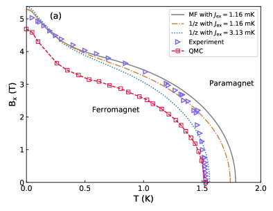
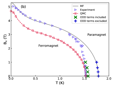
Figure 1: The full phase diagram of $\mathrm{LiHoF_{4}}$ as a function of temperature and applied transverse field. (a) A compilation of previous numerical works. Open squares are quantum Monte Carlo (QMC) results [27]. The dotted line is 1/z calculation with $J_{\text{ex}}=$3.13\text{\,}\mathrm{mK}$$ and the dot-dashed line is the same calculation with $J_{\text{ex}}=$1.16\text{\,}\mathrm{mK}$$ [28]. The solid line is a mean-field calculation [29] which uses the latter exchange value. Triangles represent results from several different experiments [4, 29, 26]. An apparent trade-off is observed between theoretical predictions that match the experimental results at low temperatures but completely fail at the low-field regime, and ones that give correct zero-field $T_{c}$ but fail to predict the correct $T_{c}(B_{x})$ dependence and give a poor match at the intermediate $B_{x}$ region. (b) Results of this paper overlaid on top of previous theoretical and experimental results. The green Xs are the numerical results of this work with off-diagonal dipolar terms included and blue plus signs are for numerical results where they are excluded. Both use $J_{\text{ex}}=$1.16\text{\,}\mathrm{mK}$$.

Results from previous studies, using various Monte Carlo (MC) techniques [27, 25] and mean-field analyses [4, 28], show a persistent discrepancy with experimental results for the $B_{x}-T$ phase diagram [4, 23, 26, 29]. Namely, when the theoretical results are fitted to the experimental results, either the zero-field critical temperature or the low-temperature–high-field regime can be made compatible with experiment, but not both. If the former is chosen, then even at small fields the $T_{c}(B_{x})$ dependence is not theoretically well reproduced, and if the latter, then the critical temperatures at low and intermediate transverse fields are significantly overestimated. The fitting is done by tuning the single free parameter representing the nearest-neighbor antiferromagnetic interaction strength, where higher values correspond to lower critical temperatures. This apparent trade-off can be clearly seen in Fig. 1(a).

Employing classical Monte Carlo simulations with variable single-spin magnetic moments, we find that the inclusion of ODD terms in the effective Hamiltonian allows for fitting $T_{c}$ at zero field using the same exchange parameter that accurately fits the data at low temperatures and high transverse fields. At the same time, we find better agreement with experimental results for the long unexplained weak dependence of $T_{c}$ on the transverse field at small fields, and the linear dependence of $T_{c}$ on $\mathrm{Ho^{3+}}$ concentration in the absence of a transverse field.

Theoretical considerations.—Off-diagonal terms of the dipolar interaction have been known to give rise to many interesting phenomena in the case of the diluted $\mathrm{LiHo_{x}Y_{1-x}F_{4}}$ in presence of an external transverse field, where they do not cancel by symmetry [20, 21, 30, 22, 19]. We argue that similar effects, arising from internal transverse fields exerted by the single ion expectation values $\expectationvalue{J^{z}_{i}}$ on the $x$ angular momentum component $J^{x}_{j}$ through terms of the form $V^{zx}_{ij}\expectationvalue{J^{z}_{i}}J^{x}_{j}$, make a significant impact on the phase diagram even in the undiluted case. The reason is that these ODD terms have a distinctly different contribution in the FM phase, where they are more likely to cancel by symmetry, than in the paramagnetic phase, where they are less likely to do so. For example, a pair of spins that lie along the $a$-axis of the crystal will exert a transverse field on spins located between them, above or below the axis connecting the two spins, if the two spins have opposite orientations. Said field acts to lower the energy of the spin on which it acts regardless of its state, thereby energetically favoring the anti-aligned configuration of its two neighboring spins. See illustrations in Fig. 2. This interaction thus constitutes a disorder-enhancing mechanism which acts to decrease the critical temperature. It requires the existence of three spins and correlation between two of them—an important aspect which will be discussed further below.

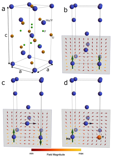
Figure 2: Crystal and magnetic structures of $\mathrm{LiHo_{x}Y_{1-x}F_{4}}$. (a) Crystal structure of $\mathrm{LiHoF_{4}}$. Only the $\mathrm{F^{-}}$ ions nearest to the central $\mathrm{Ho^{3+}}$ site are shown. (b) Correlated spins, more abundant in the FM phase, induce a field with vanishing transverse component on their common intermediate neighbor. (c) Spins in opposite orientations, more abundant in the PM phase, induce a nonzero transverse magnetic field on the third spin. (d) When one of the $\mathrm{Ho^{3+}}$ ions is replaced by an $\mathrm{Y^{3+}}$ ion, the remaining Ho induces a transverse field on its neighbor regardless of its orientation. Thick green arrows indicate dipole moments, small colored arrows show the magnetic field generated by the two magnetic dipoles and a narrow black arrow qualitatively indicates the magnitude of the transverse component of the magnetic field exerted on the middle ion. The full effect captured in the simulation is a result of the transverse field not just on the middle ion, but on all other ions in the system. For further details on this point see Supplemental Material [31].

Another effect of the transverse fields is to decrease the absolute value of $\expectationvalue{J^{z}}$ for the two lowest single-ion electronic energy states, by mixing them with the higher electronic states. This also contributes to the reduction of $T_{c}$ just by reducing the dominant $zz$ dipolar term proportional to $\expectationvalue{J^{z}}^{2}$. This mechanism of the correlation induced enhancement of the transverse field, by its nature, is not likely to be captured in any sort of mean-field-like analysis as it depends on the spatial fluctuations of the states. We posit that including the ODD terms is necessary to explain the previously mentioned discrepancies between theory and experiment.

Numerical details.—In order to examine the effect of ODD terms on the phase diagram of $\mathrm{LiHo_{x}Y_{1-x}F_{4}}$ we perform Monte Carlo simulations using an effective Hamiltonian derived building upon the work of Chakraborty et al. [27], but keeping the ODD terms. In this way we get an effective Hamiltonian,

$$\begin{split}H_{\text{eff}}&=\sum_{i}V_{C}(\hat{\boldsymbol{J}}_{i})-g_{L}\mu_{B}\sum_{i}\hat{\boldsymbol{B}}_{i}\cdot\hat{\boldsymbol{J}}_{i}\end{split}$$ (1)

where

$$\hat{B}^{x}_{i} =B_{x}-g_{L}\mu_{B}\sum_{j\neq i}V^{zx}_{ij}\hat{J}^{z}_{j}$$

$$\hat{B}^{y}_{i} =-g_{L}\mu_{B}\sum_{j\neq i}V^{zy}_{ij}\hat{J}^{z}_{j}$$ (2)

$$\hat{B}^{z}_{i} =-\frac{1}{2}g_{L}\mu_{B}\sum_{j\neq i}V^{zz}_{ij}\hat{J}^{z}_{j}-\frac{J_{\text{ex}}}{2g_{L}\mu_{B}}\sum_{j\in NN}\hat{J}^{z}_{j}$$

act as effective internal fields when taking their expectation values, thereby transforming Eq. (1) to an effective Hamiltonian for the single spins $i$. The $V_{C}(\boldsymbol{J}_{i})$ term is a crystal field potential which imposes an Ising easy axis along the $c$ axis of the crystal, with a first excited state at $\sim$10\text{\,}\mathrm{K}$$ above the ground-state doublet [28]. $V_{ij}^{\mu\nu}$ is the magnetic dipole interaction, $J_{\text{ex}}$ is the nearest-neighbor exchange interaction coupling constant, $\mu_{B}=$0.6717\text{\,}\mathrm{K}\text{\,}{\mathrm{T}}^{-1}$$ is the Bohr magneton and $g_{L}=\frac{5}{4}$ is a Landé g-factor. $\boldsymbol{J}_{i}$ are angular momentum operators of the $\mathrm{Ho^{3+}}$ ions. See further details on the derivation of the effective Hamiltonian in the Supplemental Material .

Since the $\mathrm{Ho^{3+}}$ ions retain their Ising character up to transverse fields well above the critical transverse field [30] we model a single-ion as a 2-state Ising system under an applied field exerted by all other ions in the system, as well as the external field. This applied field not only shifts the energies of the two states, but also modifies the single ion magnetic moments $\expectationvalue{J^{z}}$ associated with them. These are the magnetic moments which in turn exert magnetic fields on other ions. Therefore, each site has two possible states, $\ket{\uparrow}$ and $\ket{\downarrow}$, and each of these has two quantities of interest associated with it: local energy $\bra{\uparrow(\downarrow)}H_{\text{single-site}}\ket{\uparrow(\downarrow)}$ and magnetic moment $\bra{\uparrow(\downarrow)}J^{z}\ket{\uparrow(\downarrow)}$ where

$$H_{\text{single-site}}=V_{C}(\hat{\boldsymbol{J}})-g_{L}\mu_{B}\boldsymbol{B}\cdot\hat{\boldsymbol{J}}.$$ (3)

The method of employment of the effective Hamiltonian within the Monte Carlo simulations is detailed in the ”Numerical Methods” section of the Supplemental Material [31].

Results.—Figure 1(b) shows the $B_{x}-T$ phase diagram of $\mathrm{LiHoF_{4}}$. Our results, with ODD terms included and excluded, both use the exchange parameter $J_{\text{ex}}=$1.16\text{\,}\mathrm{mK}$$ suggested in Refs. [28, 29] which corresponds to the fitting at low temperatures and high transverse fields. It is easy to see that the simulation with ODD terms excluded corresponds to the mean-field calculation, while the results with ODD terms included are in close agreement with the experimental results, for zero and small transverse fields.

Thus, the inclusion of the ODD terms results in good agreement with experiment at zero transverse field without the need to choose $J_{\text{ex}}$ that is in clear disagreement with experiment at lower temperatures and higher transverse fields. For finite but small transverse fields we find that the decrease in $T_{c}$ due to the ODD terms is maintained. We emphasize that our simulation is a classical MC simulation, but one that allows for varying magnetic moments due to the influence of transverse fields. Therefore, the $T_{c}(B_{x})$ dependence in our results is a consequence of the renormalization of individual magnetic moments due to the quantum coupling of each of the Ising doublet states to higher excited electronic states, as opposed to quantum fluctuations between the two Ising doublet states. Hence, our model is expected to be valid at low fields $B_{x}\lesssim$1\text{\,}\mathrm{T}$$ where quantum fluctuations are small [30].

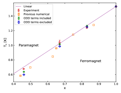
Figure 3: Transition temperature, $T_{c}$, vs. $\mathrm{Ho^{3+}}$ concentration, $x$, phase diagram from different sources: experimental from Ref. [29] (triangles), numerical from Refs. [17, 38] (squares) and this work with ODD terms included (circles) and ODD terms excluded (diamonds). A dotted line shows the mean-field prediction (linear). Numerical results from this work are scaled so that they agree with the experimental $T_{c}(x=1)=$1.53\text{\,}\mathrm{K}$$. The results with ODD terms included use $J_{\text{ex}}=$1.16\text{\,}\mathrm{mK}$$, while the results with ODD terms excluded use $J_{\text{ex}}=$3.91\text{\,}\mathrm{mK}$$, as suggested, e.g. in Ref. [25].

Another facet of the incomplete quantitative understanding of this material has to do with the phase diagram of $\mathrm{LiHo_{x}Y_{1-x}F_{4}}$ as a function of the $\mathrm{Ho^{3+}}$ concentration $x$ at zero applied field. At moderate to high concentrations ($x\gtrsim 0.4$) experiments show a linear dependence of $T_{c}$ on $x$, in agreement with the mean-field prediction [29, 15, 37], whereas the available numerical work seems to indicate a steeper decline of $T_{c}$ as $x$ is reduced [38, 17].

We note here that the inclusion of the ODD terms in the effective low energy Hamiltonian of the system leads to an effective 3-spin interaction, proportional to the anti-correlation of two spins and the existence of the third. We thus expect this term to depend strongly on Ho concentration, allowing for its distinction from the excess antiferromagnetic exchange used to parameterize the system, and for better agreement with the experimental $x-T$ phase diagram. In Fig. 3 we present our results for $T_{c}$ as function of Ho concentration $x$ in the presence of ODD terms and exchange parameter $J_{\text{ex}}=$1.16\text{\,}\mathrm{mK}$$, and in the absence of ODD terms and $J_{\text{ex}}=$3.91\text{\,}\mathrm{mK}$$. Indeed, the results with ODD terms included show milder reduction of $T_{c}$ with decreased concentration, in better agreement with the experimental findings of $T_{c}(x)=xT_{c}(x=1)$.

An additional microscopic indication of the effect of ODD terms can be obtained by inspecting the distribution of local transverse fields. Figure 4 shows the distribution of $B_{x}$ at the end of the simulation, when the system has reached thermodynamic equilibrium, for simulations where ODD terms are included and where they are excluded, yet still considered at the end of the simulation for the calculation of the effective transverse fields. It is clear that, at a given temperature, when ODD terms are included the distribution of $B_{x}$ becomes wider. This is expected, since when ODD terms are included, configurations that maximize internal transverse fields become more energetically favorable and are thus more abundant at any given temperature.

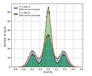
Figure 4: Distribution of local $B_{x}$ at thermodynamic equilibrium for system size $L=7$ with zero external transverse field and at $x=1$. The temperatures used, around $T=$1.66\text{\,}\mathrm{K}$$, are below $T_{c}$ when ODD terms are excluded and above $T_{c}$ when ODD terms are included. The black vertical lines at the end of each bar are standard errors. For each distribution a solid smooth line is plotted as a guide to the eye, obtained by convolution of the bin values with a Gaussian function. Where ODD terms are excluded, they are nevertheless considered at the end of the simulation for obtaining these effective transverse fields. One can clearly see that when ODD terms are included, the distribution of $B_{x}$ is wider than when they are excluded—the peak at $B_{x}=0$ is lower, compensated by higher values at the exterior. This is an indication of the ODD induced mechanism at work. Configurations maximizing internal transverse fields become more energetically favorable and thus for any given temperature they are more common.

Lastly, in order to demonstrate the effect of the ODD terms on the full $B_{x}-T$ phase diagram we pursue a simplified approach, assuming the main difference between the FM and PM phases relevant to the effectiveness of the ODD-induced mechanism is the width of the distribution of local transverse fields. For simplicity, we assume that the FM phase is characterized by a vanishing width of this distribution, while the PM phase is characterized by a finite width $h$ which we take to be $0.4\ \mathrm{T}$, i.e. the field exerted on a spin by its two nearest neighbors along the $x$ or $y$ directions while they are in opposite orientations from each other. Unsurprisingly, this is also approximately the value of the secondary peaks in Figure 4. In both phases the distribution of local transverse fields is centered around the value of the external field $B_{x}$. Hence, on average half of the spins experience a local transverse field $B_{x}+h$ and the other half $B_{x}-h$. This is true even though at $B_{x}>0$ the former option is more energetically favorable, because, owing to the crystal’s mirror symmetry, any spin which generates a positive local field at some site also generates a negative local field at another site. Thus, we estimate the energy reduction of the PM phase due to the ODD interactions, as $\Delta E(B_{x})=E(B_{x})-\left[E(B_{x}-h)+E(B_{x}+h)\right]/2$, where, for simplicity, we take $E(B_{x})$ to be the average of the two lowest eigenenergies of (3) with the given $B_{x}$. Assuming that the reduction in $T_{c}$ due to the inclusion of ODD terms, $\Delta T_{c}$, is proportional to the energy reduction $\Delta E(B_{x})$, we find the appropriate factor by demanding $\Delta T_{c}(B_{x}=0)=T_{c}^{\mathrm{MF}}(0)-T_{c}^{\mathrm{exp}}(0)\approx 1.79-1.53\approx 0.25\ \mathrm{K}$. Using this scaling factor we apply a $B_{x}$-dependent shift $\Delta T_{c}(B_{x})$ to the mean-field phase boundary to obtain an approximate phase boundary with the effect of ODD terms included, as presented in Figure 5.

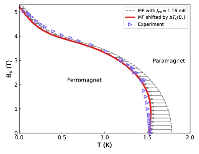
Figure 5: FM-PM phase transition line in the temperature-transverse field plane, as obtained by simple mean-field [29] (dashed gray line) and by including the $T_{c}$-reducing effect of ODD terms (solid red line). Horizontal gray arrows indicate the application of $\Delta T_{c}(B_{x})$ to the mean-field result. Triangles denote the same experimental data also shown in Fig. 1.

Discussion.—We have shown here that the description of anisotropic dipolar systems by the Ising model, and in the presence of a transverse field by the transverse field Ising model, is essentially insufficient. Even for the pure system off-diagonal dipolar terms induce an effective three spin interaction, enhancing paramagnetic fluctuations and lowering the critical temperature. We have analyzed the effect of the ODD terms on the relation between critical temperature and both transverse field and dilution, thereby addressing unanswered puzzles regarding discrepancies between theory and experiment. Our results at small fields are obtained with the same exchange parameter used to fit the phase transition at low temperatures and high transverse fields, and produce improved fitting to experimental data at finite transverse fields and as a function of Ho concentration. Thus, our results point to the need to include the quantum fluctuations induced by the off-diagonal terms in any theoretical consideration, classical and quantum, of anisotropic dipolar systems. Examples are classical and quantum annealing protocols, and a comprehensive quantum modeling of the system required to establish its full phase diagram.

Supplemental Material: The Effect of Intrinsic Quantum Fluctuations on the Phase Diagram of Anisotropic Dipolar Magnets

I Effective Hamiltonian with offdiagonal dipolar (ODD) terms included

Pure $\mathrm{LiHoF_{4}}$ forms a tetragonal structure with lattice constants $a=5.175\ \mbox{\AA}$ and $c=10.75\ \mbox{\AA}$, as shown in Fig. 2a of the main text. There are four $\mathrm{Ho^{3+}}$ ions per unit cell which form a lattice with a basis with coordinates $(0,0,\frac{1}{2})$, $(0,\frac{1}{2},\frac{3}{4})$, $(\frac{1}{2},\frac{1}{2},0)$ and $(\frac{1}{2},0,\frac{1}{4})$ [23]. The complete Hamiltonian of $\mathrm{LiHoF_{4}}$ in a transverse magnetic field is given by [27, 23]

$$H=\sum_{i}V_{C}(\boldsymbol{J}_{i})-g_{L}\mu_{B}\sum_{i}B_{x}J_{i}^{x}+\frac{1}{2}(g_{L}\mu_{B})^{2}\sum_{i\neq j}V_{ij}^{\mu\nu}J_{i}^{\mu}J_{j}^{\nu}+J_{\text{ex}}\sum_{\left\langle i,j\right\rangle}\boldsymbol{J}_{i}\cdot\boldsymbol{J}_{j}+A\sum_{i}(\boldsymbol{I}_{i}\cdot\boldsymbol{J}_{i})$$ (S.1)

where $V_{ij}^{\mu\nu}$ is the magnetic dipole interaction, $V_{ij}^{\mu\nu}=\frac{\mu_{0}}{4\pi}\frac{\delta^{\mu\nu}|\vec{r}_{ij}|^{2}-3(\vec{r}_{ij})^{\mu}(\vec{r}_{ij})^{\nu}}{|\vec{r}_{ij}|^{5}}$. $J_{\text{ex}}$ is the nearest-neighbor exchange interaction coupling constant. $\mu_{B}=$0.6717\text{\,}\mathrm{K}\text{\,}{\mathrm{T}}^{-1}$$ is the Bohr magneton, $g_{L}=\frac{5}{4}$ is a Landé g-factor, and $\mu_{0}$ denotes vacuum permeability. $\boldsymbol{J}_{i}$ are angular momentum operators of the $\mathrm{Ho^{3+}}$ ions. $A$ is the hyperfine interaction strength, and $\boldsymbol{I}_{i}$ is the nuclear spin operator, where the total $\mathrm{Ho}$ nuclear spin is $I=\frac{7}{2}$. The $\mathrm{Ho^{3+}}$ ions may be randomly substituted by nonmagnetic $\mathrm{Y^{3+}}$ ions to form $\mathrm{LiHo_{x}Y_{1-x}F_{4}}$. The crystal field term $V_{C}(\boldsymbol{J}_{i})$ imposes an Ising easy axis along the $c$ axis of the crystal, with a first excited state at $\sim$10\text{\,}\mathrm{K}$$ above the ground-state doublet [28].

Following an approach analogous to that of Chakraborty et al. [27] we recast the full Hamiltonian (S.1) as an effective transverse-field Ising model Hamiltonian, but keep the neglected ODD terms. Of the diagonal dipolar terms, we keep only the $zz$ interactions which have been established as the most dominant, but we also keep the off-diagonal interaction terms. The dipolar interaction is invariant under both $i\leftrightarrow j$ and $\mu\leftrightarrow\nu$. We also use the fact that $\commutator{J_{i}^{x}}{J_{j}^{z}}=0$ and $\commutator{J_{i}^{y}}{J_{j}^{z}}=0$ when $i\neq j$. In accordance with previous results we also keep only the $zz$ term among the three exchange interaction terms. Additionally, we neglect the hyperfine interaction, as it was found, at least within mean field approximation, not to cause a significant difference in the $B_{x}-T$ phase diagram in the vicinity of the classical phase transition [4]. The result is the effective Hamiltonian, given in Eq. (1) in the main text, which acts on the full 17-dimensional Hilbert space of the electronic angular momentum. The 2-state Ising space is created anew at each MC operation by determining the two lowest energy states and choosing one of them by the MC rules.

II Numerical Methods

In order to construct approximate many-body states of the full system, we diagonalize the single-site Hamiltonian for each of the sites, given some arbitrary initial set of magnetic moments. Using the magnetic moments obtained for each spin, the fields (The Effect of Intrinsic Quantum Fluctuations on the Phase Diagram of Anisotropic Dipolar Magnets) and ergo single-site Hamiltonians (3) are updated, and the process is repeated until convergence. Convergence is assumed when the absolute difference between the assigned magnetic moment and the magnetic moment dictated by the local field, averaged over all sites, is smaller than $\epsilon_{\text{tol}}=5\times 10^{-3}\left[\mu_{B}\right]$. Within this process, each spin is assumed to be either ”up” or ”down”, as set by the MC simulation, and only the magnitude of its magnetic moment is adjusted. The process is performed following each MC spin-flip. In effect we neglect quantum many-body effects such as entanglement, and instead consider each ion separately. Nevertheless, the single ion is treated exactly by diagonalization of its Hamiltonian in a manner that is self-consistent with all other ions. This method is somewhat similar to the approach described in Ref. [32] under the name inhomogeneous mean-field (iMF), with one important difference. We do not replace the $J^{z}$ operators in the Hamiltonian with their thermal averages but with their quantum mechanical expectation values. Thus we allow the MC simulation to sample thermal fluctuations which are required for the described mechanism to come into effect.

The determination of the single-site energy and magnetic moment is performed as follows: The Hamiltonian (3) is diagonalized numerically and its two low energy levels are designated $\ket{\alpha}$ and $\ket{\beta}$ such that $E_{\alpha}<E_{\beta}$. Next, the states $\ket{\alpha}$ and $\ket{\beta}$ are identified as $\ket{\uparrow}$ or $\ket{\downarrow}$ according to their $\expectationvalue{J^{z}}$ in the following manner: If $\expectationvalue{J^{z}}{\alpha}>\expectationvalue{J^{z}}{\beta}$ then $\ket{\alpha}\equiv\ket{\uparrow}$ and $\ket{\beta}\equiv\ket{\downarrow}$ and vise versa otherwise. Hybridization between the $\ket{\uparrow}$ and $\ket{\downarrow}$ states is suppressed due to the hyperfine interaction [18, 30], which we approximately take into account by introducing an artificial longitudinal field in the determination of $\expectationvalue{J^{z}}$ that ensures the $\ket{\uparrow}$ and $\ket{\downarrow}$ are not significantly hybridized by the transverse field: For each applied local field, $(B_{x},B_{y},B_{z})$, the $B_{z}$ component is replaced by $1.1\times\sqrt{B_{x}^{2}+B_{y}^{2}}$ for the purpose of obtaining the magnetic moment. The effect of this process can be seen in Supplementary Figure S1. In practice the energy and magnetic moment are calculated as described on a fixed grid of $B_{x}$, $B_{y}$ and $B_{z}$ from which they are linearly interpolated during the simulation.

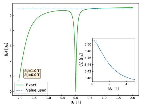
Figure S1: The magnetic moment $\expectationvalue{J^{z}}$ of the ”up” state of a single $\mathrm{Ho^{3+}}$ ion as a function of the applied $B_{z}$ magnetic field, for an applied $B_{x}=$1\text{\,}\mathrm{T}$$ field. The solid green line shows the ”exact” result (without the hyperfine interaction), which shows significant hybridization when $B_{z}$ is smaller than $B_{x}=$1\text{\,}\mathrm{T}$$. The dashed blue line shows the value used in this work, chosen as described in the text. The inset shows how this value changes as $B_{x}$ is varied.

Periodic boundary conditions are used, and the dipolar interaction $V_{ij}^{\mu\nu}$ is calculated using the Ewald summation method without a demagnetization term [16, 33].

We use the parallel tempering Monte Carlo method [34]. To determine the transitions at a given $x$ and $B_{x}$ we use the finite-size correlation length [35, 16],

$$\xi_{L}=\frac{1}{2\sin(k_{\text{min}/2})}\left[\frac{\left[\expectationvalue{m^{2}(0)}_{T}\right]_{\text{av}}}{\left[\expectationvalue{m^{2}(\boldsymbol{k}_{\text{min}})}_{T}\right]_{\text{av}}}-1\right]^{\frac{1}{2}}$$ (S.2)

where

$$m(\boldsymbol{k})=\frac{1}{N}\sum_{i=1}^{N}\expectationvalue{J_{i}^{z}}_{\psi}\exp(-i\boldsymbol{k}\cdot\boldsymbol{R}_{i}).$$ (S.3)

Here $\expectationvalue{.}_{T}$ refers to a thermal average, $\left[.\right]_{\text{av}}$ to a disorder average and $\expectationvalue{.}_{\psi}$ to a quantum mechanical expectation value. $\boldsymbol{R}_{i}$ is the location of the site $i$ and $\boldsymbol{k}_{\text{min}}=(\frac{2\pi}{L},0,0)$. The finite-size correlation length divided by the linear system size $L$ has a known scaling form,

$$\frac{\xi_{L}}{L}\sim\tilde{X}\left(L^{1/\nu}(T-T_{c})\right)$$ (S.4)

so that for $T=T_{c}$ it is independent of the system size $L$. Hence, if a transition exists, curves for different system sizes should cross at the critical temperature. We simulate systems of linear sizes $L=6,7,8$. To find $T_{c}$ we assume the scaling function (S.4) can be approximated by a third-order polynomial close to the critical point: $f(x)=p_{0}+p_{1}x+p_{2}x^{2}+p_{3}x^{3}$ (where $x=L^{1/\nu}(T-T_{c})$), and perform a global fit for the six free parameters, $p_{0}\ldots p_{3}$, $\nu$ and $T_{c}$ using the Levenberg-Marquardt algorithm. All 17 individual plots showing the analysis are presented in Supplementary Figures S2-S5. Statistical errors are estimated using the bootstrap method [36]. See Supplementary Tables 1-2 for numerical results with statistical errors.

Equilibration is verified by logarithmic binning of the data, i.e. the simulation time in terms of MC sweeps is successively increased by a factor of 2, and observables are averaged over that time. When all observables of interest in three consecutive bins agree within error bars, the simulation is deemed equilibrated [36].

For each value of $x$ or $B_{x}$ the simulation is performed twice: Once with the off-diagonal dipolar terms included in the Hamiltonian (1) and once with these terms omitted so that internal transverse fields are artificially suppressed, i.e. $B^{x}_{i}=B_{x}$ and $B^{y}_{i}=0$ for all $i$ in (The Effect of Intrinsic Quantum Fluctuations on the Phase Diagram of Anisotropic Dipolar Magnets). The self-consistent calculation for the magnetic moments is performed in both cases, as a means to establish its validity.

III Simulation Parameters

Supplementary tables 1-2 present the parameters and the results of the Monte Carlo simulations performed for this work.

Supplementary Table 1: Simulation parameters at $x=1$ for different transverse fields $B_{x}$ and system sizes $L$, with ODD terms included and excluded. The equilibration/measurement times are $2^{b}$ Monte Carlo sweeps. $T_{\text{min}}$ [$T_{\text{max}}$] is the lowest [highest] temperature used and $N_{T}$ is the number of temperatures. $N_{sa}$ is the number of independent runs. All simulations use $J_{\text{ex}}=$1.16\text{\,}\mathrm{mK}$$.

ODD terms	$B_{x}\ [\rm{T}]$	L	b	$T_{\text{min}}\ [\rm{K}]$	$T_{\text{max}}\ [\rm{K}]$	$N_{T}$	$N_{sa}$	$T_{c}\ [\rm{K}]$	$\nu$
Included	0.0	6,7,8	10	1.528	1.628	24	50	1.5735(4)	0.65(1)
Excluded	0.0	6,7	10	1.738	1.838	24	50	1.7868(3)	0.59(1)
Excluded	0.0	8	11	1.738	1.838	24	50
Included	0.3	6,7,8	10	1.512	1.612	24	50	1.5668(4)	0.61(1)
Excluded	0.3	6,7,8	10	1.739	1.839	24	50	1.7800(4)	0.60(1)
Included	0.6	6,7,8	10	1.498	1.598	24	30	1.5529(5)	0.61(1)
Excluded	0.6	6,7,8	10	1.727	1.827	24	30	1.7666(5)	0.60(2)
Included	1.0	6,7,8	10	1.47	1.57	24	30	1.5226(5)	0.64(2)
Excluded	1.0	6,7,8	10	1.705	1.804	24	30	1.7502(5)	0.61(2)
Included	1.5	6,7	10	1.42	1.52	24	30	1.4713(4)	0.56(1)
Included	1.5	8	11	1.42	1.52	24	30
Excluded	1.5	6,7	10	1.67	1.77	24	30	1.7275(5)	0.62(2)
Excluded	1.5	8	11	1.67	1.77	24	30

Supplementary Table 2: Simulation parameters at $B_{x}=0$ for different dilutions $x\leq 1$ and system sizes $L$, with ODD terms included and excluded. The equilibration/measurement times are $2^{b}$ Monte Carlo sweeps. $T_{\text{min}}$ [$T_{\text{max}}$] is the lowest [highest] temperature used and $N_{T}$ is the number of temperatures. $N_{sa}$ is the number of independent runs.

$x$	ODD terms	$J_{\text{ex}}\ [\rm{mK}]$	L	b	$T_{\text{min}}\ [\rm{K}]$	$T_{\text{max}}\ [\rm{K}]$	$N_{T}$	$N_{sa}$	$T_{c}\ [\rm{K}]$	$\nu$
1.0	Included	1.16	6,7,8	10	1.528	1.628	24	50	1.5735(4)	0.65(1)
0.83	Included	1.16	6,7,8	10	1.04	1.54	24	200	1.302(2)	0.67(4)
0.67	Included	1.16	6,7,8	10	0.78	1.28	24	350	1.044(2)	0.66(4)
0.46	Included	1.16	6	11	0.39	0.89	24	1000	0.656(2)	0.70(3)
0.46	Included	1.16	7,8	12	0.39	0.89	24	1000
1.0	Excluded	3.91	6,7,8	10	1.463	1.563	24	30	1.5177(5)	0.59(1)
0.83	Excluded	3.91	6,7,8	10	0.991	1.491	24	200	1.241(2)	0.68(4)
0.67	Excluded	3.91	6,7	10	0.724	1.224	24	350	0.978(2)	0.64(4)
0.67	Excluded	3.91	8	11	0.724	1.224	24	350
0.46	Excluded	3.91	6	11	0.354	0.854	24	1000	0.594(2)	0.65(2)
0.46	Excluded	3.91	7	12	0.354	0.854	24	1000
0.46	Excluded	3.91	8	13	0.354	0.854	24	1000

IV Finite-Size Scaling analysis

This section presents the results of the finite size scaling analysis used to obtain $T_{c}$ from each simulation. For each simulation, the value of $B_{x}$ and $x$ is set, and then a range of temperatures around $T_{c}$ is simulated for several system sizes. These simulations are used to obtain the averages required to calculate the finite-size correlation length $\xi_{L}$ which is used in the finite-size scaling method to obtain an exact estimate of $T_{c}$. Supplementary Figures S2-S5 show the finite-size scaling results. Despite expected corrections to scaling arising from the relatively small system sizes, all figures show reasonable collapse to a universal curve.

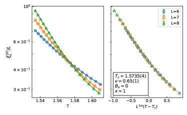
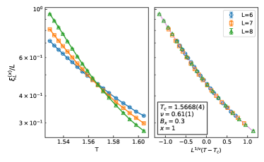
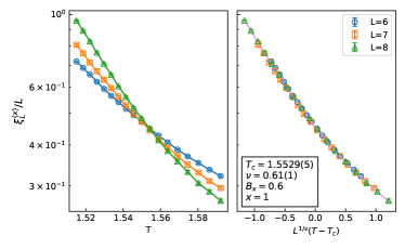
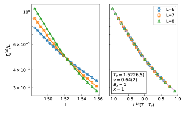
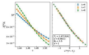
Figure S2: Finite size scaling results for simulations with ODD terms included at $x=1$ and $J_{\text{ex}}=$1.16\text{\,}\mathrm{mK}$$. Each graph is divided in two: the left side shows the raw results with the curves for different system sizes crossing at $T_{c}$ and the right side shows the same results with the $T$ axis rescaled showing a collapse onto a universal curve. The parameters for each simulation are listed within the figures.

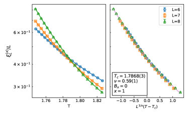
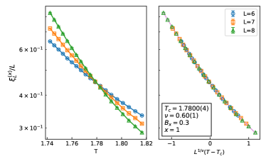
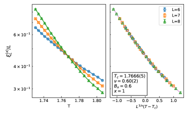
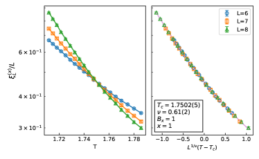
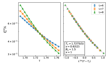
Figure S3: Finite size scaling results for simulations with ODD terms excluded. Each graph is divided in two: the left side shows the raw results with the curves for different system sizes crossing at $T_{c}$ and the right side shows the same results with the $T$ axis rescaled showing a collapse onto a universal curve. The parameters for each simulation are listed within the figures.

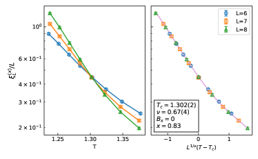
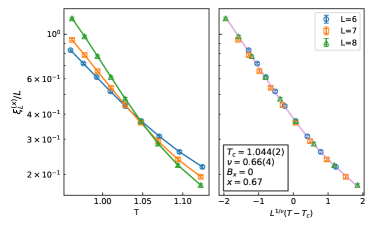
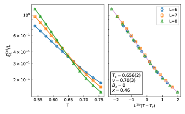
Figure S4: Finite size scaling results for simulations with ODD terms included at $x\leq 1$ and $J_{\text{ex}}=$1.16\text{\,}\mathrm{mK}$$. Each graph is divided in two: the left side shows the raw results with the curves for different system sizes crossing at $T_{c}$ and the right side shows the same results with the $T$ axis rescaled showing a collapse onto a universal curve. The parameters for each simulation are listed within the figures.

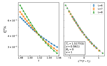
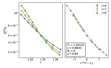
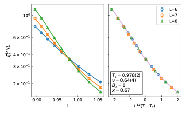
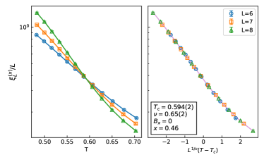
Figure S5: Finite size scaling results for simulations with ODD terms excluded at $x\leq 1$ and $J_{\text{ex}}=$3.91\text{\,}\mathrm{mK}$$. Each graph is divided in two: the left side shows the raw results with the curves for different system sizes crossing at $T_{c}$ and the right side shows the same results with the $T$ axis rescaled showing a collapse onto a universal curve. The parameters for each simulation are listed within the figures.

V Estimation of the Effective Interaction

The excess change in the energy of the system resulting from the offdiagonal dipolar (ODD) interactions can be viewed, to some extent, as a change in the effective longitudinal (zz) pair interactions. This effective change in the pair interactions is specific to each pair, is dependent on the specific spatial configuration at finite concentration, on transverse magnetic field, and to some extent on the specific configuration of all spins in the system. Yet, it is useful to calculate it in some specific configurations to allow estimation of the contribution of the offdiagonal terms to the energy of the system, and thus to $T_{c}$. To calculate the effective interaction due to the ODD mechanism, we take as one example a ferromagnetic system of all spins, except two, in the up state. We then calculate the energy of the full system for four different configurations of these 2 spins, $E(\uparrow\uparrow)$, $E(\uparrow\downarrow)$, $E(\downarrow\uparrow)$, $E(\downarrow\downarrow)$, where the energy is calculated using $H_{\text{eff}}$ given in Eq. (1) in the main text, with magnetic moments calculated self consistently as described in the text. The interaction between the two spins is then given by

$$J=\frac{1}{4}\left[E(\uparrow\uparrow)+E(\downarrow\downarrow)-E(\uparrow\downarrow)-E(\downarrow\uparrow)\right]$$

which is a result of the direct longitudinal dipolar interaction, the (nearest-neighbor) exchange interaction and the effective excess interaction due to the ODD mechanism. By repeating the above calculation with and without offdiagonal dipolar terms and subtracting one from the other, we get an estimate of the excess interaction due to the ODD mechanism $J_{\text{eff}}\equiv J(\text{ODD included})-J(\text{ODD excluded})$.

This effective interaction is calculated for pairs of spins along the x axis, along the z axis and for nearest neighbors (which can be seen in Fig. 2a in the main text). Results are obtained for a system of linear size $L=14$, where dipolar interactions are calculated using the Ewald method. For nearest neighbors the effective interaction is $J_{\text{eff}}=-31\ \mathrm{mK}$ (ferromagnetic), for the two closest spins along the x axis it is $J_{\text{eff}}=14\ \mathrm{mK}$ (antiferromagnetic), and for the two closest spins along the z axis it is $J_{\text{eff}}=11\ \mathrm{mK}$ (antiferromagnetic). These values amount to roughly 7-23% of the standard longitudinal dipolar interactions of the respective pairs. Similar results are obtained for an average over a random distribution of the spins.