TTML: tensor trains for general supervised machine learning
Abstract
This work proposes a novel general-purpose estimator for supervised machine learning (ML) based on tensor trains (TT). The estimator uses TTs to parametrize discretized functions, which are then optimized using Riemannian gradient descent under the form of a tensor completion problem. Since this optimization is sensitive to initialization, it turns out that the use of other ML estimators for initialization is crucial. This results in a competitive, fast ML estimator with lower memory usage than many other ML estimators, like the ones used for the initialization.
1 Introduction
This paper proposes a new way to use tensor networks, in particular, tensor trains (TT) or matrix product states (MPS), as machine learning (ML) estimators for general supervised learning. While tensors networks have been applied in a variety of machine learning tasks, there has been much less attention on how to use them for general labeled datasets. Indeed, a popular area of applications of low-rank tensors is in deep learning where tensors can be used for compressing layers thereby lowering storage costs and increasing inference speed; see, e.g., [Tjandra et al., 2017, Novikov et al., 2015]. They are also used in [Dai and Yeung, 2006] to learn embeddings of very high-dimensional data so that traditional ML techniques can then be applied to the lower-dimensional embeddings. Alternatively, high dimensionality can also be introduced on purpose when representing additional higher-order interactions between data as a tensor; see, e.g., [Novikov et al., 2017, Perros et al., 2017]. Finally, tensor completion in particular is useful for recovering missing high-dimensional data [Liu et al., 2013, Kressner et al., 2014, Hong et al., 2020]. All of these works have in common that tensors are used for tasks that are formulated from the start as a discrete tensor. In addition, the rationale in these applications for using low-rank tensors is in compressing high-dimensional data. For general datasets of smaller dimensionality, on the other hand, it is not clear how an ML estimator can be represented by a discrete tensor and what the benefit of low rank is. The main contribution of this paper is to close this gap.
Our method takes a different direction than the applications mentioned above. Instead of using low-rank tensors to model relatively simple relations on very high-dimensional data, we use them to model complex non-linear patterns in low-dimensional data. In particular, we will learn a discretized version of a function on a suitable finite grid. The value of this function on each grid cell can then be encoded by an order tensor. Both training and storing a dense tensor of this type is infeasible, and we shall use low-rank tensor decompositions to make the problem computationally feasible. We propose to use TTs for this purpose, since they can be efficiently trained from data using a Riemannian tensor completion algorithm. On a high level, this idea is similar to [Kargas and Sidiropoulos, 2020b, Kargas and Sidiropoulos, 2020a] where CP tensors are used to learn functions after discretization. However, their reported performance is worse than what we achieved on the same datasets, possibly due to the numerical difficulties in optimizing CP tensors.
We focus on two aspects: the discretization of the feature space, so that a discrete tensor can be used as estimator, and the learning of the estimator in a low-parametric family of tensors by local optimization. The motivation to use low-rank tensors for this task came from the identification of decision trees as sums of elementary tensors. We will show that, while decision trees naturally lead to simple low-rank tensors, one can actually learn better estimators within the same family that outperform the classical estimators with respect to model complexity and inference speed.
1.1 Tensor completion as ML estimator
As explained above, the main idea in this paper is to show that a low-rank tensor can be used to obtain a general purpose ML estimator that learns certain functions from training data. To see which functions can be represented by a tensor, we first discretize the feature space . Such a discretization can be done using a set of thresholds for each feature , with the convention
| (1) |
These thresholds divide into bins of the form . The set of all these thresholds thus divides into a grid (this is described in some more detail in Section 2). Then a tensor together with the thresholds defines a function that is locally constant on each grid cell. More precisely, is defined at as
| (2) |
Here, denotes the th entry of . The notation for the -dimensional entries of the tensor is defined analogously.
We thus consider a parametric family of functions that are constant on an irregular grid defined by thresholds . Supposing for the moment that is given, we can learn the tensor , and hence the function , using training data by minimizing an empirical loss function. This leads to the following tensor completion problem:
Problem 1.1.
Let a set of thresholds , and training data be as above. We define the regression tensor completion problem as minimizing the least-squares loss
| (3) |
where is a closed subset of the space of tensors of (relatively) small dimension (that is, a ‘tensor format’). For (binary) classification tasks where , we instead consider the classification tensor completion problem, which minimizes the cross-entropy loss
| (4) |
where is the sigmoid function. These two loss functions correspond respectively to the Gaussian and Bernoulli distributions in the context of [Hong et al., 2020], and their work also states several more potential loss functions that can be used in this context.
1.2 Main approach and outline of the paper
Solving Problem 1.1 in a good way is difficult in general. In this paper, we present practical strategies to solve this problem so that we obtain useful and competitive ML estimators on real-world data. Our approach consists of four main ‘ingredients’, which can more or less be chosen separately:
-
1.
A discretization of the feature space, or equivalently, a set of thresholds .
-
2.
The choice of tensor format .
-
3.
An algorithm to iteratively minimize the loss.
-
4.
A heuristic to initialize the tensor for the minimization algorithm.
Feature space discretization.
A good discretization of the feature space is essential when learning a discrete tensor as ML estimator. As an example and motivation, we first study decision trees in Section 2. They naturally lead to a feature space discretization, since they can be losslessly represented as a tensor in low parametric form (more concretely, as a CP tensor). Choosing the discretization of the feature space is strictly speaking not part of the (classical) tensor completion problem, but it is nevertheless essential to obtain good results in the setting of prediction or classification using tensors. While the induced partitioning of decision trees can effectively be used as discretization of the feature space with tensor regression, we found that the most effective discretization of the feature space is obtained by binning the data in roughly equally sized bins along each axis. We discuss the choice of discretization more detail in Section 5.3.
Tensor format.
There are many possibilities for the tensor subset and a popular choice is a low-rank format. For example, tensor networks that are based on a tree are well suited for optimization since they can be locally optimized using alternating strategies or Riemannian optimization; see [Bachmayr et al., 2016] and [Uschmajew and Vandereycken, 2020]. Examples of such networks are Tucker tensors, TTs, and hierarchical tensors. In addition, the closure of such tensors of a certain rank is easily parametrized. In this paper, we choose as the set of TTs since it is a format that scales well to higher dimensions and is relatively straightforward to implement. Finally, despite the representation of a decision tree as a CP, the set of tensors of bounded CP rank is not a closed set and its closure is not easily parametrized, which makes it more challenging for numerical treatment.
Optimization algorithm.
To optimize the least-squares or cross-entropy loss in the TT format, we will use Riemannian conjugate gradient descent (RCGD) as described in Section 4.1. Other common algorithms to optimize TTs are alternating least-squares (ALS) and DMRG, but in our experiments they lead to very ill-conditioned subproblems when applied to real-world data. This is because these two methods require a minimal amount of data samples for each tensor slice. The datasets we use have relatively few data points that are not uniformly distributed, which puts severe restrictions on the size of the TT we can use with ALS and DMRG. This issue is described in some more detail in Remark 4.1. The RCGD algorithm does not suffer from this problem and is much more effective in solving Problem 1.1.
Initialization.
While RCGD is very effective in finding good local minima for Problem 1.1, it needs to be properly initialized. Unless the rank of the TT is very low, the tensor completion problem has many ‘bad’ local minima. One way to deal with this issue is to start solving the tensor completion problem with a very low rank TT, and then adaptively increase the rank while resolving. While this gives decent results, we found that a much more effective initialization is obtained by fitting the TT to match a pre-trained estimator such as a random forest. We perform this fitting step using the TT-cross algorithm [Oseledets and Tyrtyshnikov, 2010, Savostyanov and Oseledets, 2011] as described in Section 4.2. Initialization can be performed with any kind of ML estimator. After further optimization of the loss, we can then match and sometimes beat the performance of the chosen estimator when measured by inference speed or validation loss, while using less parameters. This is shown empirically in Section 5
1.3 Related work
As mentioned in the introduction, learning ML estimators for general labeled datasets using low-rank tensors was also proposed in [Kargas and Sidiropoulos, 2020a, Kargas and Sidiropoulos, 2020b]. The biggest difference with the current paper is that these works use CP tensors and more sophisticated ML techniques like bagging and boosting. However, the performance of the ML estimators based on CP is considerably worse than ours on TT. It is well known [Hackbusch, 2012] that optimizing over CP tensors is more challenging numerically: alternating minimization can suffer from long stagnation before convergence, known as swamping, and many robust optimization techniques, like cross approximations and Riemannian optimization, are not directly available in CP since the format is not based on nested matricizations. We therefore conjecture that using TT tensors (or general tensor networks based on nested matricizations) is crucial for obtaining good ML estimators.
When learning the ML estimators based on TT, we use several existing techniques that have become standard practice. In particular, after discretization we are left with a tensor completion problem over the set of bounded rank TT tensors. There exist many methods for this problem, mostly based on local optimization, hard thresholding or convex relaxations; see, e.g. [Signoretto et al., 2014, Grasedyck et al., 2015, Rauhut et al., 2017, Grasedyck and Krämer, 2019]. For reasons that we explain in Remark 4.1, we chose the Riemannian optimization method from [Steinlechner, 2016].
For initialization of the Riemannian optimization method, we use the TT-cross approximation method from [Oseledets and Tyrtyshnikov, 2010, Savostyanov and Oseledets, 2011, Savostyanov, 2014]. Recently, a parallelized version of this algorithm was developed in [Dolgov and Savostyanov, 2020] which could improve the efficiency also for our setting. The idea of using TT-cross on a surrogate model so that all the fibers of the tensor are available was first proposed in [Kapushev et al., 2020]. There, the authors use a Gaussian process on a given incomplete tensor so that TT-cross can generate an initial guess for a tensor completion algorithm. We generalize this idea by fitting other ML estimators as surrogate model, like boosted trees, random forests or shallow neural networks; see [Hastie et al., 2009] for an overview of these classical ML estimators.
In contrast to most works (see our introduction and the overviews [Cichocki et al., 2017, Song et al., 2018]), the tensors in this paper only appear after a discretization of the feature space determined by the labelled data set. Discretizations are of course always needed when a discrete tensor approximates an infinite dimensional function. Tensor products of one dimensional discretizations, like Fourier series, naturally give high-order tensors; see, e.g, [Wahls et al., 2014, Bigoni et al., 2016, Imaizumi and Hayashi, 2017]. Another possibility is tensorizations of very fine discretizations of low dimensional functions using finite elements; see, e.g., [Kazeev, 2015]. Approximation rates of these continuous analogs of TT within certain function classes are available in [Bigoni et al., 2016, Schneider and Uschmajew, 2014, Kazeev and Schwab, 2017, Griebel and Harbrecht, 2021]. When learning an ML estimator from a relatively small data set, however, these continuous tensor approximations are not suitable since the underlying functions are significantly less smooth. As example we give a random forest, which corresponds to a piecewise constant partitioning of the high-dimensional domain. This only allows for very simple discretizations, like quantile binning or k-means, as was one in [Dougherty et al., 1995]. In case of image data, other possibilities for discretizations that lead to low-rank tensors are one-hot encoding or using fixed parametric families of functions, like wavelets; see [Cohen et al., 2016, Razin et al., 2021]. However, these also rely on the fact that images form a large dataset with a large degree of correlation between the features (pixels). This is not the case for our setting.
2 Motivation: Decision trees as low-rank tensors
We recall decision trees and show how they can be represented as a low-rank tensor. This serves as motivation to consider more general ML models represented by low-rank tensors. We refer to [Hastie et al., 2009] for a broader introduction into decision trees.
A (binary) decision tree represents a recursive binary partitioning of the feature space into labeled axis-aligned regions. In particular, at a non-leaf node of the tree, we split into the two regions and for some feature index and threshold . Since a single feature can be used to split multiple times, its associated thresholds are indexed by . At each leaf , we associate a label or ‘decision’ . To determine the value of for some feature vector , we start at the root of the tree and evaluate its corresponding inequality for . If it is satisfied, we proceed to the left child of the root, otherwise to the right child. This process is repeated until we reach a leaf with its corresponding decision . This determines the value of . For an illustration, see Figure 1.
Each leaf corresponds to a region defined by the points satisfying the set of inequalities encountered by traveling from the root to this leaf. Such a region is always an intersection of half-spaces and is therefore box-shaped, that is, all facets are normal to an axis. Note that these regions are not necessarily bounded. The function associated to the decision tree is then given by
| (5) |
where is the set of leaves and is the indicator function of the region .
We now show that a decision tree can be represented a low-rank tensor. Indeed, as is clear from (5) and the example in Figure 1, a decision tree is a function that is piecewise constant on a partitioning of into the boxes . As explained in Section 1.1, we can thus represent with a tensor and a set of thresholds . In fact, we can directly take over the thresholds from a decision tree, as long as we respect the ordering convention (1). Up to a trivial reordering, this can of course always be done. We have thus defined the set of all thresholds for all features .
It remains to construct the tensor so that the function defined in (2) coincides with the decision tree , that is, . It is not hard to see that this means that the elements of have to be the decision values . Note that many entries of will be the same, since each region is typically divided into multiple grid cells. In the example of Figure 1, we have that corresponds to the region where takes value . Leaf 7 corresponds to the region and thus , , and have, for example, the same value . The complete tensor in Figure 1 is given by its two slices as follows:
Having obtained a tensor from , we now show that is of low rank. We will do this by writing as a sum of at most elementary tensors that are of rank one, where is the set of leaves in the decision tree. These elementary tensors are obtained in terms of the active thresholds at each leaf. Each leaf corresponds to a region
where possibly and . We define a threshold to be active at the leaf if . For convenience, we formally set . For example, in the decision tree of Figure 1, the active thresholds for leaf are . For each feature and leaf , we then define the vector entry-wise as
For our example, we obtain , , and . Consider now the tensor
which is clearly of rank at most one. It is readily verified using (2) that then is supported on where it has constant value . Hence, from (5) we see that
| (6) |
allows us to represent the decision tree as .
The CP rank of is the minimal number of summands of non-zero elementary tensors needed to express . The formula above shows that the CP rank of is at most , but it is in fact lower if the tree is not linear. This is because if two leaves share the same parent, then is of rank 1. Indeed, if the parent of and were split for feature , then we have that for all and thus
The CP rank of is therefore also bounded by the number of nodes that have a leaf attached rather than just the number of leaves. In general, this is just an upper bound. For example, the tensor associated to the decision tree shown in Figure 2 is of rank 2 since it satisfies
where is the th standard basis vector.
Remark 2.1.
Even though the CP rank has a useful upper bound, there is no similar upper bound on the Tucker rank. The Tucker rank of is a tuple encoding the minimal dimensions of spaces such that . Depending on the tree structure, we can in general have that the Tucker rank is maximal: . Furthermore, the singular values are on the same order as the weights , and hence do not decay fast. This means that these tensors cannot be well-approximated (or compressed) using a HOSVD decomposition.
From Remark 2.1 above we conclude that compressing the tensor associated to a decision tree in a tensor format like CP or Tucker is probably not useful. For example, as we will also note in Remark 3.1, we cannot efficiently express most decision trees in the TT format either. Furthermore, in ML estimation tasks, we care about minimizing the test error and in principle not about compression error. However, we will see that the underlying tensor from a decision tree can be useful as initialization when solving Problem 1.1; see Section 4.2.
Finally, we remark that we can also see random forests as tensors in the CP format. Recall that in a random forest we independently train a number of decision trees, each on a different subset of the training data. We then average out the predictions of all the decision trees to obtain a useful estimator. This is therefore a weighted sum of decision trees, each of which we can represent by a CP tensor. Similarly in a boosted forest, we train decision trees sequentially and combine them with a weighted sum as well. It is important to note however that the set of thresholds is different for each decision tree. To represent the random/boosted forest as a CP tensor we have to merge the sets of thresholds of all the constituent decision trees. The result is that both the CP rank and the number of thresholds increase linearly with the number of trees in the forest, resulting in a quadratic increase in storage costs.
3 The tensor train decomposition
The tensor train (TT) decomposition is a popular low-rank decomposition of tensors. We recall basic properties of this decomposition and describe a solution to the tensor completion problem for this format. Most of the content in this section is fairly standard; see, e.g., [Hackbusch, 2012, Oseledets, 2011]. For the tensor completion problem and Riemannian structure of the TT format we mainly follow [Steinlechner, 2016].
A TT decomposition of a tensor consists of order 3 core tensors of the form
We denote the slice , which is for each a matrix of size . The tensor is then decomposed element-wise as
| (7) |
This decomposition is shown in Penrose graphical notation below. The labels on the edges indicate dimensions, and the two one-dimensional edges are omitted.
The tuple is called the TT-rank. The set of all tensors that can be written as a TT of exactly rank form a (non-closed) embedded submanifold . In Section 3.2 we will study the Riemannian geometry of this manifold. The closure of consists of all TT of rank at most rank , which we denote by . Each TT in can be written in the form (7). We note that is not a submanifold.
3.1 Orthogonalization and rank truncation
An important property of the TT decomposition is that we can orthogonalize the cores. Each core has a left matricization and a right matricization by flattening or ‘matricizing’ the order 3 tensor to a matrix. The core is left-orthogonal if the columns of are orthonormal: . Similarly, right-orthogonal means . We call a TT orthogonalized at mode if all cores are left-orthogonal for and right-orthogonal for . A TT is left-orthogonalized if it is orthogonalized at mode , similarly it is right-orthogonalized if it is orthogonalized at mode .
If a TT is orthogonalized at mode , then we also have that , where is obtained by contracting all cores with . This is because on the very left we have which is already a matrix, and thus . Similarly for , we have . This is shown below for and a TT orthogonalized at mode . This also shows that if a TT tensor is orthogonalized at mode , then we can compute its Euclidean norm as . See Figure 3 for a graphical illustration of this idea.
Any TT can easily be orthogonalized through a QR-procedure. To left-orthogonalize, for example, we perform the following procedure to each core from left to right: Compute the QR decomposition of the left matricization . Set to the tensorisation of . Multiply the matrix into the tensor . These steps are also shown below.
If we want to instead right-orthogonalize a TT, then we perform the orthogonalization right-to-left, and each individual step in the orthogonalization is transposed with respect to the picture above. Using that a QR factorization of an matrix costs flops, the cost of a complete left-to-right or right-to-left sweep is given by
| (8) |
To orthogonalize at mode we left-orthogonalize all the cores with and right-orthogonalize those with .
Instead of a QR decomposition, one can also use the singular value decomposition (SVD) above. While SVD is slightly more expensive than QR, it allows us to reduce the ranks of a given TT in a quasi-optimal manner. For example, in the diagram below, if is the SVD and the rank- truncated SVD, then we update by the tensorisation of , and we absorb into the next core:
Doing this in a left-to-right fashion to all cores both left-orthogonalizes the TT and reduces its TT-rank from to . We will denote this truncation by the map which is quasi-optimal in the sense that
| (9) |
where denotes the best approximation of in the closed subset ; see [Hackbusch, 2012, §12.2.7]. Assuming the SVD of an matrix costs flops, computing costs
| (10) |
Remark 3.1.
A tensor in CP format can be written easily in TT format; see [Hackbusch, 2012, §8.5.2]. In particular, let
as in (6) be a CP tensor that represents a decision tree, then we can define the cores of the corresponding (left-orthogonal) TT as
This is unfortunately not very useful in practice. The TT rank is equal to with the CP rank of , which typically scales linearly with the size of the decision tree, as discussed in Section 2. Furthermore, the HOSVD gives in practice very bad approximations, since most singular values are . This is because the vectors have norm and are close to orthogonal. Any reasonable truncation of by HOSVD will thus have a very high TT-rank. Nevertheless, and quite surprisingly, we can still get useful approximations of random forests (sums of decision trees) with small TT-rank using the TT-cross algorithm. This is discussed in Section 4.2.
3.2 Manifold structure
To perform Riemannian optimization on a manifold , we need three main ingredients: a description of the tangent bundle and its metric, a retraction , and a vector transport map ; see, e.g., the general overview [Absil et al., 2008]. For the manifold of TTs, the usual choice for retraction and vector transport are the HOSVD truncation and the orthogonal projection onto the tangent space. We will briefly recall the description of these ‘ingredients’ as introduced by [Steinlechner, 2016].
Tangent vectors.
Let be the left-orthogonal cores of a TT tensor . Similarly, are its right-orthogonal cores. Then tangent vectors are given by tensors of the form
| (11) | ||||
where has the same shape as . We call the tensors first-order variations. If they satisfy the gauge condition for all , then they are uniquely defined from (11) for each tangent vector .
Note that the representation (11) of is itself a rank- TT: thanks to the gauge condition, we can indeed write
| (12) |
Metric.
As metric for , we restrict the Euclidean metric on to . The gauge condition also guarantees a simple expression for the metric. Namely if then
| (13) |
Retraction.
The decomposition (12) of a tangent vector is also important for computing the retraction by HOSVD. If , then as well, since
| (14) |
To obtain a retraction, we can thus define
| (15) |
where the map was explained in Section 3.1. Since the TT representation (14) is explicitly available at no cost, the retraction can be computed in flops; see (10) with the substitutions and .
Tangent space projection.
Given a tensor , we want to compute its orthogonal projection onto directly in the representation (11). This operation is needed for transporting a tangent vector to a different tangent space, and for calculating the Riemannian gradient of a loss function. In the first case, is a tensor of TT-rank at most as was noted above, while in the second, it is a sparse tensor since Problem 1.1 is a tensor completion problem.
We first explain how to compute efficiently when has TT-rank and (non-normalized) cores . Recall that and are the left- and right-orthogonal cores of . First, we contract and without its th core:
| (16) |
The result of contracting this network is a tensor of shape . Next, we compute for
| (17) |
so that respects the gauge condition . For , we can take above so that . The tuple now defines using (11).
For efficiency reasons, it is worthwhile to pre-compute all products in a left-to-right sweep, and all products in a right-to-left sweep. Then, we obtain by contracting , and . Using the assumption , an easy calculation shows that the total cost in flops of the vector transport is bounded by
| (18) |
A different strategy is needed when is sparse, that is, only for . Different from (16), the (non-normalized) first-order variation is now obtained from the contraction with an unstructured :
| (19) |
Applying the gauge conditions is again done as in (17). We therefore only need to explain how to compute the slices for . Let
| (20) |
By inspecting (19), we then obtain
| (21) |
Since is a row vector and is a matrix for , the first product in brackets is a row vector. Since the second product is also a row vector, we thus decompose as a sum of rank-one matrices. By abuse of notation, we write for the vector with all values of for . Similarly, we write for the matrix with columns given by for . We denote the matrix similarly. Then (21) becomes
| (22) |
The matrices and can be computed efficiently for each in, respectively, a left-to-right and right-to-left sweep at a cost of flops. The total cost of computing using (22) is therefore given by
| (23) |
Applying the gauge conditions (17) costs another flops, assuming that the left- and right-orthogonalizations , are already available.
Remark 3.2.
The method above of projecting a sparse is mathematically equivalent to the one introduced in [Steinlechner, 2016], but ours is significantly more efficient in practice. Instead of computing many rank-one updates in an outer loop over as in (21), we group these operations into matrix products and tensor contractions as in (22). The latter is much faster on modern hardware.
4 TTML: TT-based ML estimator
We now describe how to solve the completion Problem 1.1 using TTs to obtain a competitive ML estimator that we call TTML. The training procedure for TTML is summarized below in Algorithm 1. After training, inference is performed by evaluating the function defined by (2).
4.1 TT completion by RCGD
For the minimization of the loss function in Problem 1.1, we will use Riemannian conjugate gradient descent (RCGD). For a standard regression task, the loss function satisfies
| (24) |
Here , denotes the training data, and is defined by (2). Let us consider the index set
| (25) |
which also defines multi-index sets as used in (20).
To optimize (24) with RCGD, we compute the derivative of . It is a sparse tensor with non-zero entries indexed by and
| (26) |
If we want to minimize the cross-entropy loss (4), then we have instead
| (27) |
with the sigmoid function. Note that there may be multiple data points corresponding to the same set of indices . If this happens we simply sum over these data points in (26) and (27).
We summarize the general procedure of RCGD in Algorithm 2.
As line search, we use standard Armijo backtracking111We also experimented with non-monotone Armijo backtracking as well as backtracking using the Wolfe conditions, but this gave no improvement in performance for our application. applied to . Even in the context of Riemannian optimization, this can be implemented fairly easily; see, e.g., [Absil et al., 2008]. In particular, thanks the rigidity of , we have . In addition, choosing a good initial step size for backtracking algorithm leads to a significant difference in performance. In [Steinlechner, 2016], the initial step is computed based on an exact minimizer of the line search objective without retraction,
| (28) |
We found that for our setting a better initial step is the (type-I) Barzilai-Borwein (BB) step size. Let and . Then, as in [Wen and Yin, 2013], we define
| (29) |
This does however require computing the vector transport of the gradient, which is unnecessary in .
For the conjugate gradient scalar , we either use steepest descent , or the Riemannian Fletcher-Reeves choice222Both choices lead to similar performance.
| (30) |
Remark 4.1.
The more standard ALS and DMRG approaches for solving this problem do not work well in this context. In the ALS scheme we optimize the TT one core at a time. The ALS objective for each core decouples into problems for each slice of the form
| (31) |
where, by abuse of notation, is the th number such that . This is a least-squares problem in the entries of , but unfortunately it is often ill-conditioned. Observe that the slice is of size . If thus , the problem is underdetermined. Additionally, the indices are not uniformly distributed, and it often happens that multiple data points end up in the same grid-cell. This further reduces the effective number of data points available for determining the slice . In practice this means ALS can only be used if the number of thresholds is small for each feature, and if the ranks are small. In our experiments, regularization techniques somewhat helped, but the lack of data remained a large issue. For DMRG, the situation is even worse, since the optimization problem for the supercores decouples even further and there are even less effective data points available per supercore. Gradient based algorithms do not suffer from this issue, and for this reason we have chosen to solve the tensor completion problem using Riemannian conjugate gradient descent instead.
4.2 Initialization from existing estimators with TT-cross
The Riemannian algorithm described in Section 4.1 is only effective with a good initialization. Unless the number of thresholds and TT-rank is small, the RCGD algorithm tends to end up in ‘bad’ local minima with random initialization. We therefore propose to generate an initial guess by fitting a TT to an existing ML estimator trained on the data. Good estimators are, for example, random forests or neural networks. Fitting a TT to an estimator is different from the tensor completion Problem 1.1 because we can evaluate at any point we wish. The goal is therefore to solve333In practice, the norm in (32) is approximated as a sum over a finite amount of points.
| (32) |
We will do this using the TT-cross approximation algorithm [Oseledets and Tyrtyshnikov, 2010, Savostyanov and Oseledets, 2011]. There are two versions of the TT-cross algorithm, based on ALS or on DMRG that optimize one or two cores, respectively, of the TT at a time. A full sweep of the ALS (DMRG) version costs () flops and () evaluations of the function , respectively. While the DMRG version is more expensive, it requires significantly fewer iterations to converge, can adapt the ranks, and tends to result in a better approximation of the function . We recommend using the DMRG version unless it is prohibitively expensive. In all the experiments described in Section 5 we have used the DMRG version.
A similar idea to improve the initialization of tensor completion problems was proposed in [Kapushev et al., 2020] where TT-cross was used in combination with a Gaussian process (GP) trained on the same data. In our setting, we found that it is worth exploring different ML estimators for this initialization step since the final accuracy obtained depends strongly on the combination of the training data and the ML estimator. This will be discussed further in Section 5.
4.3 Overview of computational cost
We give an overview of the computational costs in flops of all the operations needed for the TTML estimator. For simplicity we assume that the TT is of order with uniform TT-rank and uniform dimensions . Furthermore, we assume so that . For RCGD, we denote the number of (Armijo) line search steps used by . Finally, is the number of data points in the training set.
| Operation | Complexity (flops) | Eq. |
| Orthogonalization of TT | (8) | |
| HOSVD from rank to | (10) | |
| Inference (per sample) | (7) | |
| Projection of sparse gradient | (23) | |
| Retraction | (10, 15) | |
| Vector transport | (18) | |
| RCGD (one step) | ||
| ALS TT-cross (full sweep) | flops and function evaluations | |
| DMRG TT-cross (full sweep) | flops and function evaluations |
Most importantly, observe that all of the operations are linear in and . Since typically scales as to avoid overfitting, we obtain a complexity of , like other tensor completion algorithms; see, e.g., [Steinlechner, 2016]. We note that the term in prediction is due to computing the indices associated to data points. Since the thresholds are sorted, this is done using binary search. The cost of one step of RCGD is computed as the sum of one sparse gradient projection, retractions and predictions, one vector transport, and one orthogonalization. All other operations needed for RCGD are at most .
5 Experiments
The source code and documentation for all the experiments described in this paper are available as a Python package at https://github.com/RikVoorhaar/ttml. All the experiments were performed on a desktop computer with an 8-core Intel i9-9900 using version 1.0 of the software. Our implementation of the TT-cross algorithm is a translation to Python of the MATLAB implementation in the TT-toolbox [Oseledets, 2014].
5.1 General setup and datasets used
We have collected several datasets from the UCI Machine Learning Repository [Dua and Graff, 2017] to evaluate our TTML estimator. All the datasets have a relatively small number of features, and a modest number of samples. The used datasets are summarized in Table 1.
| Dataset | Task | #Features | #Samples |
|---|---|---|---|
| AI4I 2020 | Class. | 6 | 10000 |
| Airfoil Self-noise | Regr. | 5 | 1503 |
| Bank Marketing | Class. | 16 | 45211 |
| Adult | Regr. | 14 | 32561 |
| Concrete compressive strength | Regr. | 8 | 1030 |
| Default of credit card | Class. | 23 | 30000 |
| Diabetic Retinopathy Debrecen | Class. | 19 | 1151 |
| Electrical Grid Stability | Class. | 13 | 10000 |
| Gas Turbine Emissions | Regr. | 10 | 36733 |
| Online Shoppers | Class. | 17 | 12330 |
| Combined Cycle Power Plant | Regr. | 4 | 9568 |
| Seismic-bumps | Class. | 15 | 2584 |
| Shill Bidding | Class. | 9 | 6321 |
| Wine quality | Regr. | 11 | 4898 |
As baseline estimators, we chose random forest and boosted trees, since they both consistently perform very well on all the datasets. Implementations were provided by the Python packages scikit-learn [Pedregosa et al., 2011] and XGBoost [Chen and Guestrin, 2016], respectively.
For all experiments, we created a random 70/15/15 train/validation/test split, where the validation data is used for early stopping and hyperparameter optimization. For each estimator and dataset, we first optimized the most relevant hyperparameters using the validation split444Using Bayesian optimization as in [Bergstra et al., 2013] and kept only the best result. Using these best hyperparameters, the estimators were fitted and evaluated again on the same train/validation/test splits, and the error on the test set was recorded. Due to the relatively low number of samples in our datasets, this resulted in high variance. We therefore repeated this experiment 12 times on different train/validation/test splits, and we report the mean and standard deviation of the loss over these 12 splits. All estimators are evaluated on the same splits of the data, and the same procedure is used for both the baseline and our TTML estimators.
For the TTML estimator, the main hyperparameters are the TT-ranks, number of thresholds and estimator used for initialization. We used a uniform maximum number of thresholds for each feature, and a uniform TT-rank for each core. The thresholds were chosen to divide the data values in roughly equally sized bins along each axis, since this generally gives the best performance (as will be discussed in Section 5.3). We trained four different TTML estimators that were each initialized with TT-cross (with fixed rank) using the following estimators555We also tried Gaussian Processes as in [Kapushev et al., 2020] but the results were not competitive for our datasets.: random forests, multi-layer perceptrons (shallow neural networks) with one or two layers(s), and boosted trees. This was then followed by several steps of RCGD to minimize the loss as explained in Problem 1.1. During RCGD we monitored performance on the validation dataset for early stopping.
The results on all datasets are shown in Table 2. From the table it is clear that the performance of TTML depends strongly on which estimator was used during the TT-cross initialization. With the best initialization, TTML only improves on XGBoost once, but it does match or beat the random forest for 3 datasets. Overall, TTML does not seem to improve the baseline estimators if one is only interested in test error. However, as we will investigate below, TTML is superior in error versus model complexity and inference speed.
Some of the datasets666The Concrete compressive strength, Wine quality, and Combined cycle power plant datasets, where they reported scores of respectively 29.8, 0.49, and 14.1. were also used by [Kargas and Sidiropoulos, 2020b, Kargas and Sidiropoulos, 2020a]. These authors similarly discretized ML estimators using low-rank tensors, but they use CPs instead of TTs. It is therefore interesting to compare the estimators. While TTML outperforms their reported scores on these three datasets, a direct comparison is not possible unfortunately since we do not have access to an implementation of their estimator.
| Dataset | ttml_xgb | ttml_rf | ttml_mlp1 | ttml_mlp2 | xgb | rf |
|---|---|---|---|---|---|---|
| AI4I 2020 | 0.23(15) | 0.220(68) | 0.238(98) | 0.35(15) | 0.0426(78) | 0.0490(76) |
| Airfoil Self-noise | 2.63(72) | 2.81(62) | 2.28(53) | 2.39(70) | 2.39(67) | 3.45(56) |
| Bank Marketing | 0.1911(65) | 0.1938(58) | 0.255(43) | 0.84(62) | 0.1717(43) | 0.1753(46) |
| Adult | 0.369(24) | 0.357(12) | 0.396(28) | 0.90(45) | 0.2788(76) | 0.2984(75) |
| Concrete compr. strength | 23.5(6.3) | 23.4(7.5) | 46.9(8.6) | 37(13) | 17.9(4.0) | 24.4(4.9) |
| Default of credit card | 0.59(22) | 0.59(29) | 0.83(20) | 1.04(28) | 0.4302(55) | 0.4275(60) |
| Diab. Retinopathy Debr. | 3.08(55) | 1.9(1.5) | 5.7(4.1) | 6.0(1.6) | 0.573(47) | 0.578(31) |
| Electrical Grid Stability | 0.029(23) | 0.080(64) | 0.041(23) | 0.065(33) | 0.0011(29) | 0.0171(15) |
| Gas Turbine Emissions | 0.856(59) | 1.028(86) | 2.67(29) | 3.88(89) | 0.291(12) | 0.434(26) |
| Online Shoppers | 0.79(38) | 0.58(20) | 0.60(28) | 0.83(25) | 0.222(11) | 0.227(11) |
| Comb. Cycle Power Plant | 11.4(1.4) | 11.6(1.3) | 14.6(5.3) | 12.5(1.5) | 8.7(1.1) | 11.2(1.2) |
| Seismic-bumps | 0.85(11) | 1.12(54) | 1.89(51) | 0.75(31) | 0.228(28) | 0.219(28) |
| Shill Bidding | 0.041(31) | 0.195(63) | 0.097(69) | 0.081(49) | 0.0075(50) | 0.0213(36) |
| Wine quality | 0.510(20) | 0.474(19) | 1.53(49) | 3.4(2.1) | 0.388(13) | 0.380(13) |
5.2 Test error, model complexity, and inference speed
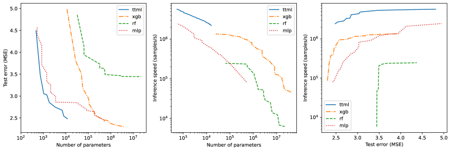
We now investigate the relation between model complexity, inference speed, and test error in more detail for the airfoil self-noise dataset.
Model complexity for the estimators is defined as the number of parameters in the model. For TTML, we used the number of entries in all the cores of the TT, which is with the number of thresholds used per feature and the TT-rank. For a random forest and a boosted tree model, the number of parameters is proportional to the number of trees and the number of nodes in the tree. For both models, the decision trees are encoded as an array, and the number of parameters is computed as the sum of the sizes of these arrays for each tree in the random/boosted forest. The number of parameters of a multi-layer perceptron is computed as the total number of elements used for all the weights and biases.
We trained the TTML estimator with TT-ranks ranging from 2 to 19, and maximum number of thresholds per feature ranging from 15 to 150. For each pair of rank and number of thresholds, we initialized as explained in the previous section with TT-cross. The best model in terms of test error was kept (this initialization has no effect on the number of parameters or the inference speed). Furthermore, we trained a random forest, boosted tree, and MLP model for a large range of hyperparameters on the same data.
The results of these comparisons are visible in Figure 4. We can see that for a given test error our TTML model consistently performs faster, and needs less parameters. This suggests that our estimator is potentially useful in low-memory applications where inference speed of a pretrained model is favored over accuracy.
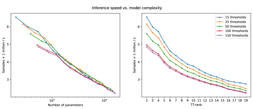
In Figure 5 we show the relation between number of parameters, TT-rank and inference speed in more detail. In theory, inference speed scales as ; see Section 4.3. This influence on is reflected in our experimental results. The dependence on is only logarithmic since a binary search is used to associate a correct multi-index to each data point. In practice, however, we observe a larger dependence on than theoretically expected. This is likely because, in our implementation, inference is bound by memory speed, and memory usage depends linearly on .
5.3 Feature space discretization methods
As explained in Section 1.1, the feature space is discretized using the thresholds so that a discrete tensor can be used as an ML estimator. Choosing a good feature space discretization turns out to be important for the quality of the estimator. The dependence of the estimator on the discretization is not differentiable, and we only have heuristic methods for choosing the thresholds.
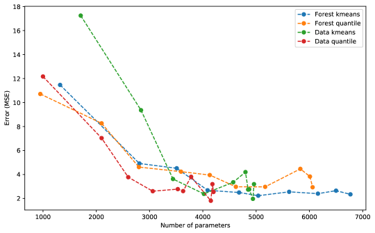
A straightforward way to choose the thresholds is to pick them such that they divide the data values for each feature into equally sized bins in terms of frequency. That is, we choose them according to quantile statistics of the data. Another discretization relies on choosing the thresholds using k-means to solve a one-dimensional clustering problem for each feature; see [Dougherty et al., 1995]. Instead of dividing the feature space directly, one can also first fit a random forest or decision tree to the data, and then use the decision boundaries of the decision trees as thresholds for the discretization.
In Figure 6, we compared these four discretization methods for the airfoil self-noise dataset. In particular, we trained a random forest on the data, and then used either quantile binning or k-means clustering to select a subset of thresholds, either directly from the features or from the decision boundaries. For this data set, we see that the simplest methods, directly quantile binning of the features, works best. Since similar behavior was observed for other data sets as well, we choose this discretization in all our tests.
5.4 Ordering of the features
Some estimators, like neural networks and random forests, are insensitive to permutation of the features. This is not the case for TTML since the TT-rank of a tensor, and thus our model, depends on this ordering. In some applications with tensors, certain orderings (or more general, certain topologies of the tensor network) lead to much better approximations given a budget of parameters; see, e.g, [Ballani and Grasedyck, 2014, Bebendorf and Kuske, 2014, Grelier et al., 2019]. In this section, we show experimentally that the same phenomenon can happen for TTML. However, in our setting, we will illustrate this for the test error and not for the approximation error of the underlying tensor.
For this experiment we again used the airfoil self-noise dataset. Since it has only 5 features, we can train TTML estimators for all 120 different permutations of the features. We repeated the experiment on 30 different train/test/validation splits. For each permutation and split, we trained our estimator with 40 thresholds per feature and a TT-rank of 6. The tensor train was initialized on a random forest fit on the same training split. For each permutation the mean performance is determined.777The variance in the mean performance is modeled as with . This value of was obtained by dividing the mean sample standard deviation over all 120 permuations by the mean performance over all 120 permuations. We found that the experimental data is very consistent with this model, unlike computing sample standard deviation for each permutation separately or using a constant .
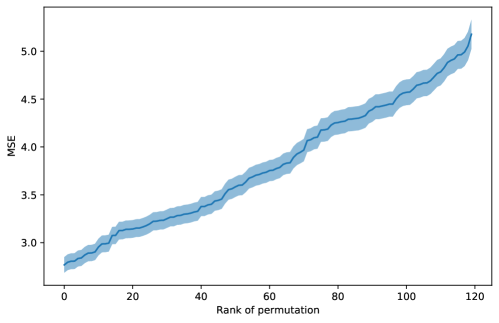
The results are shown in Figure 7. We clearly see that the ordering has a strong effect on the test error. The best 5 permutations are , whereas the 5 worst are . The only statistically significant pattern we found is that feature zero is best put at position 0 or 4, especially compared to putting this feature in the middle. Despite a non-optimal choice of hyperparameters, the performance of the best permutation beats the best performance on the ‘default’ permutation of the features shown in Table 2. It is therefore clear that a method for estimating the optimal permutation of the features would be very useful.888Such methods exists for compression of TTs (see, e.g., [Ballani and Grasedyck, 2014, Bebendorf and Kuske, 2014, Grelier et al., 2019]) but it is not clear how these ideas can be extended when one is interested in test error.
5.5 Number of thresholds and TT-rank
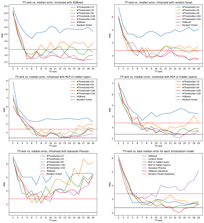
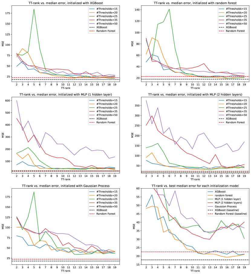
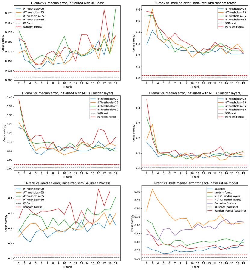
As last experiment, we investigate in more detail the dependence of the TTML estimator on the number of thresholds, the TT-rank, and the initialization method on the following datasets: airfoil self noise, concrete compressive strength, and shill bidding. The training of TTML and the baseline methods (random forest and boosted tree), the optimization of the hyperparameters and the selection of the final methods was done as in Section 5.1 for the construction of Table 2.
The results are visible for each dataset separately in Figures 8–10 further below. Most importantly, we see that the best initialization method is strongly dependent on the dataset. For example, for the airfoil self noise dataset, we obtain best performance using an MLP for initialization, whereas for the concrete compressive strength dataset it is achieved using a random forest, and for the shill bidding dataset it is XGBoost. Finally, Gaussian process based initialization is consistently the worst.
The performance is also dependent on the number of thresholds used for initialization, and the TT-rank. The optimal number of thresholds and TT rank depends on the dataset and the estimator used for initialization. Generally the error decreases with TT-rank and number of thresholds until an optimal point after which the error (slowly) increases with additional complexity. It seems that the optimal TT-rank does not depend strongly on the number of thresholds used, and these hyperparameters can therefore effectively be optimized using a coordinate descent procedure.
6 Extensions, future work, and conclusions
6.1 Extensions of TTML
The TTML estimator described in Algorithm 1 is very flexible, and can be generalized in many ways to create potentially more useful ML estimators. We will now discuss some of the more promising extensions, all of which may be studied in future work.
Topology of the network.
Problem 1.1 can be formulated for virtually any tensor format, not just TTs. An obvious generalization of the present work is therefore to replace TTs in Algorithm 1 with a general tree tensor networks, like the hierarchical Tucker (HT) format that uses binary trees. Compared to TT, more general trees sometimes results in lower complexity (ranks) at the expense of learning a much more complicated topology of the tree; see, e.g., [Ballani and Grasedyck, 2014, Bebendorf and Kuske, 2014, Grelier et al., 2019]. In order to adapt our methods to such a different tensor format, we need a good black box approximation method, and an efficient implementation of retraction and vector transport to perform RCGD (or an alternative method to efficiently solve the tensor completion problem in the given format). For the HT format, black box approximation is described in [Ballani et al., 2013], whereas (Riemannian) tensor completion for HT is described in [Da Silva and Herrmann, 2014, Rauhut et al., 2015]. Adapting our methods to the HT format should therefore be straightforward. For other tensor formats, such as CP, tensor rings or MERA, black box approximation and tensor completion may be more challenging to perform with reasonable computational and storage complexity.
Approximation of multivariate functions.
While for simplicity we have only considered approximation of univariate functions , our methods readily generalize to the multivariate case . Given data , , we can use the same discretization of as in the univariate case. We then consider the tensor completion problem for tensors . Using the same definition, the function defined by (2) now takes values in and the regression tensor completion problem 1.1 becomes
| (33) |
There is no obstruction to using the TT format (or tree tensor networks) in this context; we simply add one additional core to the TT on the right. TT-cross can still be used to perform black box approximation, and RCGD can still be used for tensor completion in this context.
Use as first layer in feedforward network.
The multivariate generalization described previously can be used as first layer in a feedforward network using backpropagation in order to improve its performance. The function can be composed with any other parametric model . Here can be any differentiable model, such as a linear model or a neural network. This results in the optimization problem
| (34) |
where is some loss function that depends on the training data . This can be efficiently optimized using gradient based methods and backpropagation. We first compute the gradients of :
| (35) |
Then similar to (26) we compute the Euclidean gradient for with respect to by
| (36) |
After projection onto the tangent space this gradient can then be used for Riemannian gradient descent as usual. Note that since is a locally constant function, the derivative a.e., and TTML therefore does not support backpropagation itself. For this reason, TTML can only be used as a first layer in a feedforward network.
6.2 Conclusions
We have described a novel general-purpose ML estimator based on tensor completion of TTs. The estimator is competitive compared to existing estimators if measured by inference speed and model complexity, for a given test error. The model is very flexible, and has several promising generalizations. This illustrates the expressive power of low-rank tensor decompositions, and their potential use in data science and statistics. From another perspective, we have also highlighted the importance of good initialization for tensor completion problems, and we have shown that using auxiliary models for initialization can improve the performance on tensor completion problems dramatically.
References
- [Absil et al., 2008] Absil, P.-A., Mahony, R., and Sepulchre, R. (2008). Optimization Algorithms on Matrix Manifolds. Princeton University Press.
- [Bachmayr et al., 2016] Bachmayr, M., Schneider, R., and Uschmajew, A. (2016). Tensor Networks and Hierarchical Tensors for the Solution of High-Dimensional Partial Differential Equations. Found Comput Math, 16(6):1423–1472.
- [Ballani and Grasedyck, 2014] Ballani, J. and Grasedyck, L. (2014). Tree Adaptive Approximation in the Hierarchical Tensor Format. SIAM J. Sci. Comput., 36(4):A1415–A1431.
- [Ballani et al., 2013] Ballani, J., Grasedyck, L., and Kluge, M. (2013). Black box approximation of tensors in hierarchical Tucker format. Linear Algebra and its Applications, 438(2):639–657.
- [Bebendorf and Kuske, 2014] Bebendorf, M. and Kuske, C. (2014). Separation of Variables for Function Generated High-Order Tensors. J Sci Comput, 61(1):145–165.
- [Bergstra et al., 2013] Bergstra, J., Yamins, D., and Cox, D. (2013). Making a Science of Model Search: Hyperparameter Optimization in Hundreds of Dimensions for Vision Architectures. In Proceedings of the 30th International Conference on Machine Learning, pages 115–123. PMLR.
- [Bigoni et al., 2016] Bigoni, D., Engsig-Karup, A. P., and Marzouk, Y. M. (2016). Spectral Tensor-Train Decomposition. SIAM Journal on Scientific Computing, 38(4):A2405–A2439.
- [Chen and Guestrin, 2016] Chen, T. and Guestrin, C. (2016). XGBoost: A Scalable Tree Boosting System. Proceedings of the 22nd ACM SIGKDD International Conference on Knowledge Discovery and Data Mining, pages 785–794.
- [Cichocki et al., 2017] Cichocki, A., Lee, N., Oseledets, I., Phan, A.-H., Zhao, Q., Sugiyama, M., and Mandic, D. P. (2017). Tensor Networks for Dimensionality Reduction and Large-scale Optimization: Part 2 Applications and Future Perspectives. Foundations and Trends® in Machine Learning, 9(6):249–429.
- [Cohen et al., 2016] Cohen, N., Sharir, O., and Shashua, A. (2016). On the Expressive Power of Deep Learning: A Tensor Analysis. In Conference on Learning Theory, pages 698–728. PMLR.
- [Da Silva and Herrmann, 2014] Da Silva, C. and Herrmann, F. J. (2014). Optimization on the Hierarchical Tucker manifold - applications to tensor completion. arXiv:1405.2096 [math].
- [Dai and Yeung, 2006] Dai, G. and Yeung, D.-Y. (2006). Tensor embedding methods. In Proceedings of the 21st National Conference on Artificial Intelligence - Volume 1, AAAI’06, pages 330–335, Boston, Massachusetts. AAAI Press.
- [Dolgov and Savostyanov, 2020] Dolgov, S. and Savostyanov, D. (2020). Parallel cross interpolation for high-precision calculation of high-dimensional integrals. Computer Physics Communications, 246:106869.
- [Dougherty et al., 1995] Dougherty, J., Kohavi, R., and Sahami, M. (1995). Supervised and Unsupervised Discretization of Continuous Features. In Prieditis, A. and Russell, S., editors, Machine Learning Proceedings 1995, pages 194–202. Morgan Kaufmann, San Francisco (CA).
- [Dua and Graff, 2017] Dua, D. and Graff, C. (2017). UCI Machine Learning Repository. https://archive.ics.uci.edu/ml.
- [Grasedyck et al., 2015] Grasedyck, L., Kluge, M., and Krämer, S. (2015). Variants of Alternating Least Squares Tensor Completion in the Tensor Train Format. SIAM Journal on Scientific Computing, 37(5):A2424–A2450.
- [Grasedyck and Krämer, 2019] Grasedyck, L. and Krämer, S. (2019). Stable ALS approximation in the TT-format for rank-adaptive tensor completion. Numerische Mathematik, 143(4):855–904.
- [Grelier et al., 2019] Grelier, E., Nouy, A., and Chevreuil, M. (2019). Learning with tree-based tensor formats. arXiv:1811.04455 [cs, math, stat].
- [Griebel and Harbrecht, 2021] Griebel, M. and Harbrecht, H. (2021). Analysis of Tensor Approximation Schemes for Continuous Functions. Foundations of Computational Mathematics.
- [Hackbusch, 2012] Hackbusch, W. (2012). Tensor Spaces and Numerical Tensor Calculus, volume 42 of Springer Series in Computational Mathematics. Springer Berlin Heidelberg, Berlin, Heidelberg.
- [Hastie et al., 2009] Hastie, T., Tibshirani, F., and Friedman, J. (2009). The Elements of Statistical Learning: Data Mining, Inference, and Prediction. Springer.
- [Hong et al., 2020] Hong, D., Kolda, T. G., and Duersch, J. A. (2020). Generalized Canonical Polyadic Tensor Decomposition. SIAM Rev., 62(1):133–163.
- [Imaizumi and Hayashi, 2017] Imaizumi, M. and Hayashi, K. (2017). Tensor Decomposition with Smoothness. In Proceedings of the 34th International Conference on Machine Learning, pages 1597–1606. PMLR.
- [Kapushev et al., 2020] Kapushev, Y., Oseledets, I., and Burnaev, E. (2020). Tensor Completion via Gaussian Process–Based Initialization. SIAM J. Sci. Comput., 42(6):A3812–A3824.
- [Kargas and Sidiropoulos, 2020a] Kargas, N. and Sidiropoulos, N. D. (2020a). Nonlinear System Identification via Tensor Completion. Proceedings of the AAAI Conference on Artificial Intelligence, 34(04):4420–4427.
- [Kargas and Sidiropoulos, 2020b] Kargas, N. and Sidiropoulos, N. D. (2020b). Supervised Learning via Ensemble Tensor Completion. In 2020 54th Asilomar Conference on Signals, Systems, and Computers, pages 196–199.
- [Kazeev, 2015] Kazeev, V. (2015). Quantized Tensor-Structured Finite Elements for Second-Order Elliptic PDEs in Two Dimensions. PhD thesis, SAM, ETH Zurich, ETH Dissertation No. 23002.
- [Kazeev and Schwab, 2017] Kazeev, V. and Schwab, C. (2017). Quantized tensor-structured finite elements for second-order elliptic PDEs in two dimensions. Numerische Mathematik.
- [Kressner et al., 2014] Kressner, D., Steinlechner, M., and Vandereycken, B. (2014). Low-rank tensor completion by Riemannian optimization. Bit Numer Math, 54(2):447–468.
- [Liu et al., 2013] Liu, J., Musialski, P., Wonka, P., and Ye, J. (2013). Tensor Completion for Estimating Missing Values in Visual Data. IEEE Transactions on Pattern Analysis and Machine Intelligence, 35(1):208–220.
- [Novikov et al., 2015] Novikov, A., Podoprikhin, D., Osokin, A., and Vetrov, D. (2015). Tensorizing Neural Networks. arXiv:1509.06569 [cs].
- [Novikov et al., 2017] Novikov, A., Trofimov, M., and Oseledets, I. (2017). Exponential Machines. arXiv:1605.03795 [cs, stat].
- [Oseledets, 2011] Oseledets, I. (2011). Tensor-Train Decomposition. SIAM J. Scientific Computing, 33:2295–2317.
- [Oseledets and Tyrtyshnikov, 2010] Oseledets, I. and Tyrtyshnikov, E. (2010). TT-cross approximation for multidimensional arrays. Linear Algebra and its Applications, 432(1):70–88.
- [Oseledets, 2014] Oseledets, I. V. (2014). TT-toolbox. https://github.com/oseledets/TT-Toolbox.
- [Pedregosa et al., 2011] Pedregosa, F., Varoquaux, G., Gramfort, A., Michel, V., Thirion, B., Grisel, O., Blondel, M., Prettenhofer, P., Weiss, R., Dubourg, V., Vanderplas, J., Passos, A., Cournapeau, D., Brucher, M., Perrot, M., and Duchesnay, É. (2011). Scikit-learn: Machine Learning in Python. Journal of Machine Learning Research, 12(85):2825–2830.
- [Perros et al., 2017] Perros, I., Wang, F., Zhang, P., Walker, P., Vuduc, R., Pathak, J., and Sun, J. (2017). Polyadic Regression and its Application to Chemogenomics. In Proceedings of the 2017 SIAM International Conference on Data Mining (SDM), Proceedings, pages 72–80. Society for Industrial and Applied Mathematics.
- [Rauhut et al., 2015] Rauhut, H., Schneider, R., and Stojanac, Ž. (2015). Tensor Completion in Hierarchical Tensor Representations. In Boche, H., Calderbank, R., Kutyniok, G., and Vybíral, J., editors, Compressed Sensing and Its Applications: MATHEON Workshop 2013, Applied and Numerical Harmonic Analysis, pages 419–450. Springer International Publishing, Cham.
- [Rauhut et al., 2017] Rauhut, H., Schneider, R., and Stojanac, Ž. (2017). Low rank tensor recovery via iterative hard thresholding. Linear Algebra and its Applications, 523:220–262.
- [Razin et al., 2021] Razin, N., Maman, A., and Cohen, N. (2021). Implicit Regularization in Tensor Factorization. arXiv:2102.09972 [cs, stat].
- [Savostyanov and Oseledets, 2011] Savostyanov, D. and Oseledets, I. (2011). Fast adaptive interpolation of multi-dimensional arrays in tensor train format. In The 2011 International Workshop on Multidimensional (nD) Systems, pages 1–8.
- [Savostyanov, 2014] Savostyanov, D. V. (2014). Quasioptimality of maximum-volume cross interpolation of tensors. Linear Algebra and its Applications, 458:217–244.
- [Schneider and Uschmajew, 2014] Schneider, R. and Uschmajew, A. (2014). Approximation rates for the hierarchical tensor format in periodic Sobolev spaces. Journal of Complexity, 30(2):56–71.
- [Signoretto et al., 2014] Signoretto, M., Tran Dinh, Q., De Lathauwer, L., and Suykens, J. A. K. (2014). Learning with tensors: A framework based on convex optimization and spectral regularization. Mach Learn, 94(3):303–351.
- [Song et al., 2018] Song, Q., Ge, H., Caverlee, J., and Hu, X. (2018). Tensor Completion Algorithms in Big Data Analytics. arXiv:1711.10105 [cs, stat].
- [Steinlechner, 2016] Steinlechner, M. (2016). Riemannian Optimization for High-Dimensional Tensor Completion. SIAM J. Sci. Comput., 38(5):S461–S484.
- [Tjandra et al., 2017] Tjandra, A., Sakti, S., and Nakamura, S. (2017). Compressing recurrent neural network with tensor train. In 2017 International Joint Conference on Neural Networks (IJCNN), pages 4451–4458.
- [Uschmajew and Vandereycken, 2020] Uschmajew, A. and Vandereycken, B. (2020). Geometric Methods on Low-Rank Matrix and Tensor Manifolds. In Grohs, P., Holler, M., and Weinmann, A., editors, Handbook of Variational Methods for Nonlinear Geometric Data, pages 261–313. Springer International Publishing, Cham.
- [Wahls et al., 2014] Wahls, S., Koivunen, V., Poor, H. V., and Verhaegen, M. (2014). Learning multidimensional Fourier series with tensor trains. In 2014 IEEE Global Conference on Signal and Information Processing (GlobalSIP), pages 394–398.
- [Wen and Yin, 2013] Wen, Z. and Yin, W. (2013). A feasible method for optimization with orthogonality constraints. Math. Program., 142(1-2):397–434.