Change-point Detection and Segmentation of Discrete Data
using Bayesian Context Trees

Abstract

A new Bayesian modelling framework is introduced for piece-wise homogeneous variable-memory Markov chains, along with a collection of effective algorithmic tools for change-point detection and segmentation of discrete time series. Building on the recently introduced Bayesian Context Trees (BCT) framework, the distributions of different segments in a discrete time series are described as variable-memory Markov chains. Inference for the presence and location of change-points is then performed via Markov chain Monte Carlo sampling. The key observation that facilitates effective sampling is that the prior predictive likelihood in each segment of the data can be computed exactly, averaged over all models and parameters. This makes it possible to sample directly from the posterior distribution of the number and location of the change-points, leading to accurate estimates and providing a natural quantitative measure of uncertainty in the results. Estimates of the actual model in each segment can also be obtained, at essentially no additional computational cost. Results on both simulated and real-world data indicate that the proposed methodology performs better than or as well as state-of-the-art techniques.

Keywords. Discrete time series, change-point detection, segmentation, piece-wise homogeneous variable-memory chains, Bayesian context trees, context-tree weighting, Markov chain Monte Carlo, DNA segmentation.

1 Introduction

Change-point detection and segmentation are important statistical tasks with a broad range of applications across the sciences and engineering. These tasks have been studied extensively for continuous-valued time series; see, e.g., Aminikhanghahi and Cook (2017); Truong et al. (2020); van den Burg and Williams (2020) for detailed reviews. Relatively less attention has been paid to discrete time series, where analogous problems naturally arise, e.g., in genetics, biomedicine, neuroscience, health system management, finance, and the social sciences (Chandola et al., 2012). For what is probably the most critical application, namely, the segmentation of genetic data, the most commonly used tools are based on Hidden Markov Models (HMMs). Since their introduction for modelling heterogeneous DNA sequences by Churchill (1989, 1992), they have become quite popular in a wide range of disciplines (Kehagias, 2004). More recently, Bayesian HMM approaches have also been proposed and used in practice (Boys and Henderson, 2004; Totterdell et al., 2017). In this paper we take a different Bayesian approach, modelling each segment of the time series as a variable-memory Markov chain.

As has been often noted, the main obstacles in the direct approach to modelling dependence in discrete time series are that: 1. ordinary, higher-order Markov chains form an inflexible and structurally poor model class; and 2. their number of parameters grows exponentially with the memory length. Variable-memory Markov chains provide a much richer and more flexible model class that offers parsimonious and easily interpretable representations of higher-order chains, by allowing the memory length to depend on the most recent observed symbols. These models were first introduced as context-tree sources in the information-theoretic literature by Rissanen (1983a, b, 1986), and they have been used widely in connection with data compression. In particular, the development of the celebrated Context-Tree Weighting (CTW) algorithm (Willems et al., 1995; Willems, 1998) is based on context-tree sources. Variable-memory Markov models were subsequently examined in the statistics literature, initially by Bühlmann and Wyner (1999); Mächler and Bühlmann (2004), under the name Variable Length Markov Chains (VLMC).

More recently, a Bayesian modelling framework, called Bayesian Context Trees (BCTs), was developed by Kontoyiannis et al. (2022, 2021); Papageorgiou and Kontoyiannis (2022) for the class of variable-memory Markov chains. As described briefly in Section 2, the BCT framework allows for exact Bayesian inference, it was found to be very effective for discrete time series, cf. (Papageorgiou et al., ), and it was also extended to general Bayesian mixture models for real-valued time series (Papageorgiou and Kontoyiannis, 2021).

The first contribution of this work, in Section 3, is the introduction of a new Bayesian modelling framework for piece-wise homogeneous discrete time series. A uniform prior is placed on the number of change-points, and an “order statistics” prior is placed on their locations (Green, 1995; Fearnhead, 2006), which penalizes short segments to avoid overfitting. Finally, each segment is described by a BCT model, thus defining a new class of piece-wise homogeneous variable-memory chains. Following Kontoyiannis et al. (2022), we observe that the models and parameters in each segment can be integrated out and show that the corresponding prior predictive likelihoods can be computed exactly and efficiently by using a version of the CTW algorithm.

The second main contribution, also in Section 3, is the development of a new class of Bayesian methods for inferring the number and location of change-points in empirical data. A collection of appropriate Markov chain Monte Carlo (MCMC) algorithms is introduced, that sample directly and efficiently from the posterior distribution of the number and the locations of the change-points. The resulting approach is quite powerful as it provides an MCMC approximation for the posterior distribution of interest, offering broad and insightful information in addition to the estimates of the most likely change-points. Finally, in Section 4, the performance of our methods is illustrated on both simulated and real-world data from applications in genetics and meteorology, where they are found to perform at least as well as state-of-the-art approaches. All our algorithms are implemented in the publicly available R package BCT (Papageorgiou et al., ), which also contains all relevant data sets.

Further connections with earlier work. Unlike many of the relevant existing methods, which mainly only obtain point estimates and may rely in part on ad hoc considerations, the present methodology comes from a principled Bayesian approach that provides access to the entire posterior distribution for the parameters of interest, in particular allowing for quantification of the uncertainty in the resulting estimates. The most closely related prior work is that of Gwadera et al. (2008), where VLMC models are used in conjunction with the BIC criterion (Schwarz, 1978) or with a variant of the Minimum Description Length principle (Rissanen, 1987) to estimate variable-memory models and perform segmentation by solving an associated Bellman equation.

There has also been a long line of works on change-point detection in the information-theoretic literature. There, piece-wise homogeneous models were first considered by Merhav (1993) and Merhav and Feder (1995), who determined the optimal cumulative log-loss (or ‘redundancy’, in the language of data compression). Starting with Willems (1996), a series of papers examined sequential change-point detection, typically (but not exclusively) for independent and piece-wise identically distributed models. These works (Shamir and Merhav, 1999; Shamir and Costello, 2000, 2001; Shamir, 2003) are primarily concerned with deriving theoretical bounds on the best achievable performance by on-line methods, and also propose sequential algorithms for change-point detection, mostly for piece-wise i.i.d. (independent and identically distributed) data. In a related but different direction, Jacob and Bansal (2008) and subsequently Juvvadi and Bansal (2013); Verma and Bansal (2019); Yamanishi and Fukushima (2018), frame the change-point detection problem as a series of hypothesis tests, performed using statistics based on data compression or entropy estimation algorithms. And an approach combining HMMs with information-theoretic ideas is adopted in Koolen and de Rooij (2013), where prediction is performed on piece-wise stationary data.

Finally, in the context of generalisations of the original CTW framework, change-point models have also been examined by Veness et al. (2012) and Veness et al. (2013), and more recently by Shimada et al. (2021), who consider optimal and practical ‘Bayes codes’ for data compression in connection with these models.

2 Background: Bayesian context trees

The BCT framework of Kontoyiannis et al. (2022), briefly outlined in this section, is based on variable-memory Markov chains, a class of models that offer parsimonious representations of $D$th order, homogeneous Markov chains taking values in a finite alphabet $A=\{0,1,\ldots,m-1\}$. The maximum memory length $D\geq 0$ and the alphabet size $m\geq 2$ are fixed throughout this section. Each model describes the distribution of a process $\{X_{n}\}$ conditional on its initial $D$ values $X_{-D+1}^{0}=x_{-D+1}^{0}$, where we write $X_{i}^{j}$ for a vector of random variables $(X_{i},X_{i+1},\ldots,X_{j})$ and similarly $x_{i}^{j}=(x_{i},x_{i+1},\ldots,x_{j})$ for a string in $A^{j-i+1}$. This is done by specifying the conditional distribution of each $X_{n}$ given $X_{n-D}^{n-1}$.

The key step in the variable-memory model representation is the assumption that the distribution of $X_{n}$ in fact only depends on a (typically strictly) shorter suffix $x_{n-j}^{n-1}$ of $x_{n-D}^{n-1}$. All these suffixes, called contexts, can be collected into a proper $m$-ary tree $T$ describing the model of the chain. [A tree here is called proper if all its nodes that are not leaves have exactly $m$ children.] For example, consider the binary tree model in Figure 1. With $D=3$, given $X_{n-3}^{n-1}=111$, the distribution of $X_{n}$ only depends on the fact that the two most recent symbols are 1’s, and it is given by the parameter $\theta_{11}$.

Figure 1: Tree model and parameters of a 3rd order variable-memory chain.

Let ${\mathcal{T}}(D)$ denote the collection of all proper $m$-ary trees with depth no greater than $D$. To each leaf $s$ of a model $T\in{\mathcal{T}}(D)$, we associate a probability vector $\theta_{s}$ that describes the distribution of $X_{n}$ given that the most recently observed context is $s$: $\theta_{s}=(\theta_{s}(0),\theta_{s}(1),\ldots,\theta_{s}(m-1))$.

Prior structure. The prior distribution on models $T\in{\mathcal{T}}(D)$ is given by,

$$\pi(T)=\pi_{D}(T;\beta)=\alpha^{|T|-1}\beta^{|T|-L_{D}(T)},$$ (1)

where $\beta\in(0,1)$ is a hyperparameter, $\alpha=(1-\beta)^{1/(m-1)}$, $|T|$ is the number of leaves of $T$, and $L_{D}(T)$ is the number of leaves of $T$ at depth $D$. This prior penalizes larger and more complex models by an exponential amount. The default choice for $\beta=1-2^{-m+1}$ is used throughout.

Given a tree model $T\in{\mathcal{T}}(D)$, an independent Dirichlet$(1/2,1/2,\ldots,1/2)$ prior is placed on the parameters $\theta=\{\theta_{s}:s\in T\}$ associated to the leaves $s$ of $T$, so that, $\pi(\theta|T)=\prod_{s\in T}\pi(\theta_{s}),$ where,

$$\pi(\theta_{s})=\pi(\theta_{s}(0),\theta_{s}(1),\ldots,\theta_{s}(m-1))\propto\prod_{j=0}^{m-1}\theta_{s}(j)^{-1/2}.$$ (2)

Likelihood. Given a tree model $T\in{\mathcal{T}}(D)$ and associated parameters $\theta=\{\theta_{s}:s\in T\}$, the induced likelihood is given by,

$$P(x|T,\theta):=P(x_{1}^{n}|T,\theta,x_{-D+1}^{0})=\prod_{i=1}^{n}P(x_{i}|T,\theta,x_{-D+1}^{i-1})=\prod_{s\in T}\ \prod_{j=0}^{m-1}\theta_{s}(j)^{a_{s}(j)},$$ (3)

where the elements $a_{s}(j)$ of each count vector $a_{s}=(a_{s}(0),a_{s}(1),\ldots,a_{s}(m-1))$ are given by, $a_{s}(j):=\mbox{\# times symbol $j\in A$ follows context $s$ in $x_{1}^{n}$}$.

Exact Bayesian inference. An important advantage of the BCT framework is that it allows for exact Bayesian inference. In particular, for a time series $x=x_{-D+1}^{n}$ consisting of observations $x_{1}^{n}$ together with an initial context $x_{-D+1}^{0}$, the prior predictive likelihood (or evidence) $P_{D}^{*}(x)$ averaged over both models and parameters, namely,

$$P_{D}^{*}(x)=\sum_{T\in{\mathcal{T}}(D)}\pi(T)\int_{\theta}P(x|T,\theta)\pi(\theta|T)d\theta,$$

can be computed exactly by the CTW algorithm (Kontoyiannis et al., 2022). This is of crucial importance, as the number of models in ${\mathcal{T}}(D)$ grows doubly exponentially in $D$. Moreover, through the BCT algorithm (Kontoyiannis et al., 2022) the maximum a posteriori probability (MAP) tree model can also be efficiently identified at essentially no additional computational cost. These features open the door to a wide range of applications, including change-point detection as studied in this work.

3 Bayesian change-point detection via Bayesian context trees

In this section, we describe the proposed Bayesian modelling framework and the associated inference methodology for discrete time series with change-points.

Each segment is modelled by a homogeneous variable-memory chain as in Section 2. Two different cases are considered: When the number of change-points $\ell$ is known a priori, and when $\ell$ is unknown and needs to be inferred as well. Consider a time series $x=x_{-D+1}^{n}$ consisting of the observations $x_{1}^{n}$ along with their initial context $x_{-D+1}^{0}$. Let $\ell$ denote the number of change-points and let $1=p_{0}<p_{1}<p_{2}<\cdots<p_{l}<p_{\ell+1}=n$ denote their locations, where we include the end-points $p_{0}=1$ and $p_{\ell+1}=n$ for convenience. We write, $\mbox{\boldmath$p$}=(p_{0},p_{1},\ldots,p_{\ell+1})$.

3.1 Known number of change-points

Piece-wise homogeneous Markov models. Suppose the maximum memory length $D$ is fixed. Given a time series $x_{-D+1}^{n}$, the number of change-points $\ell$, and their locations $\mbox{\boldmath$p$}=(p_{0},p_{1},\ldots,p_{\ell+1})$, the observations $x_{1}^{n}$ are partitioned into $(\ell+1)$ segments,

$$x(1;\mbox{\boldmath$p$})=x_{1}^{p_{1}-1},$$

$$x(j;\mbox{\boldmath$p$})=x^{p_{j}-1}_{p_{j-1}},\text{ for }j=2,3,\ldots,\ell,$$

$$x(\ell+1;\mbox{\boldmath$p$})=x_{p_{\ell}}^{n}.$$

Each segment $x(j;\mbox{\boldmath$p$})$, $1\leq j\leq\ell+1$, is assumed to be distributed as a variable-memory chain with model $T^{(j)}\in{\mathcal{T}}(D)$, parameter vector $\theta^{(j)}$, and initial context given by the $D$ symbols preceding $x_{p_{j-1}}$ (i.e., the last $D$ symbols of the previous segment). The resulting likelihood is,

$$P(x|\mbox{\boldmath$p$},\{\theta^{(j)}\},\{T^{(j)}\})=\prod_{j=1}^{\ell+1}P(x^{p_{j}-1}_{p_{j-1}}|x_{p_{j-1}-D}^{p_{j-1}-1},\theta^{(j)},T^{(j)}),$$

where each term in the product is given by (3).

Prior structure. Given the number $\ell$ of change-points, following Green (1995) and Fearnhead (2006), we place a prior on their locations $p$ specified by the even-order statistics of $(2\ell+1)$ uniform draws from $\{2,3,\ldots,n-1\}$ without replacement,

$$\pi(\mbox{\boldmath$p$}|\ell)=K_{\ell}^{-1}\prod_{j=0}^{\ell}\ (p_{j+1}-p_{j}-1),$$ (4)

where $K_{\ell}=\binom{n-2}{2\ell+1}$. This prior penalizes short segments to avoid overfitting: The probability of $p$ is proportional to the product of the lengths of the segments $x(j;\mbox{\boldmath$p$})$. For example, the prior gives zero probability to adjacent change-points in $p$, i.e., to segments with zero length.

Finally, given $\ell$ and $p$, an independent BCT prior $\pi(T^{(j)})\pi(\theta^{(j)}|T^{(j)})$ is placed on the model and parameters of each segment $j$, as in (1) and (2).

Posterior distribution. The posterior distribution of the change-point locations $p$ is,

$$\pi(\mbox{\boldmath$p$}|x)\propto P(x|\mbox{\boldmath$p$})\pi(\mbox{\boldmath$p$}|\ell),$$

with $\pi(\mbox{\boldmath$p$}|\ell)$ as in (4). To compute the term $P(x|\mbox{\boldmath$p$})$, all models $T^{(j)}$ and parameters $\theta^{(j)}$ in $P(x,\{\theta^{(j)}\},\{T^{(j)}\}|\mbox{\boldmath$p$})$ need to be integrated out. Since independent priors are placed on different segments, $P(x|\mbox{\boldmath$p$})$ reduces to the product of the prior predictive likelihoods,

$$P(x|\mbox{\boldmath$p$})=\prod_{j=1}^{\ell+1}P_{D}^{*}(x(j;\mbox{\boldmath$p$})),$$ (5)

where the dependence on the initial context for each segment is suppressed to simplify notation.

Importantly, each term in the product (5) can be computed efficiently using the CTW algorithm. This means that models and parameters in each segment can be marginalized out, making it possible to efficiently compute the unnormalised posterior $\pi(\mbox{\boldmath$p$}|x)$ for any $p$. This is critical for effective inference on $p$, as it means that there is no need to estimate or sample the variables $\{T^{(j)}\}$ and $\{\theta^{(j)}\}$ in order to sample directly from $\pi(\mbox{\boldmath$p$}|x)$, as described next.

MCMC sampler. The MCMC sampler for $\pi(\boldsymbol{p}|x)$ is a Metropolis-Hastings (Robert and Casella, 2004) algorithm. It takes as input the time series $x=x_{-D+1}^{n}$, the alphabet size $m\geq 2$, the maximum memory length $D\geq 0$, the prior hyperparameter $\beta$, the number of change-points $\ell\geq 1$, the initial MCMC state $\boldsymbol{p}^{(0)}$, and the total number of MCMC iterations $N$.

Given the current state $\boldsymbol{p}^{(t)}=\boldsymbol{p}$, a new state $\boldsymbol{p}^{\prime}$ is proposed as follows: One of the change-points $p_{i}$ is chosen at random from $\boldsymbol{p}$ (excluding the edges $p_{0}=1$ and $p_{\ell+1}=n$), and it is replaced either by a uniformly chosen position $p_{i}^{\prime}$ from the $(n-\ell-2)$ remaining available positions, with probability 1/2, or by one of its two neighbours, again with probability 1/2. [Note that the neighbours of a change-point are always available, as the prior places zero probability to adjacent change-points.]

The proposed $\boldsymbol{p}^{\prime}$ is either accepted and $\boldsymbol{p}^{(t+1)}=\boldsymbol{p}^{\prime}$, or rejected and $\boldsymbol{p}^{(t+1)}=\boldsymbol{p}$, where the acceptance probability is given by $\alpha(\boldsymbol{p},\boldsymbol{p}^{\prime})=\min\{1,r(\boldsymbol{p},\boldsymbol{p}^{\prime})\}$, where,

$$r(\boldsymbol{p},\boldsymbol{p}^{\prime})=\frac{P(x|\boldsymbol{p}^{\prime})}{P(x|\boldsymbol{p})}\times{\displaystyle\prod_{j=0}^{\ell}}\frac{(p_{j+1}^{\prime}-p_{j}^{\prime}-1)}{(p_{j+1}-p_{j}-1)}.$$

Importantly, the fact that the terms $P(x|\boldsymbol{p})$ and $P(x|\boldsymbol{p}^{\prime})$ can be computed efficiently by the CTW algorithm is what enables this sampler to work effectively.

3.2 Unknown number of change-points

In most applications the number of change-points $\ell$ is not known a priori, and needs to be treated as an additional parameter to be inferred. As before, given the number and location of the change-points, each segment is modelled by a variable-memory chain.

Prior structure. Given the maximum possible number of change-points $\ell_{\rm max}\geq 1$, we place a uniform prior for $\ell$ on $\{0,1,\ldots,\ell_{\rm max}\}$, and, given $\ell$, the rest of the priors on $\boldsymbol{p}$, $\{T^{(j)}\}$ and $\{\theta^{(j)}\}$ remain the same as in Section 3.1. The uniform prior is a common choice for $\ell$ in such problems, as the Bayesian approach implicitly penalizes more complex models by averaging over a larger number of parameters, resulting in what is sometimes referred to as “automatic Occam’s Razor” (Smith and Spiegelhalter, 1980; Kass and Raftery, 1995; Rasmussen and Ghahramani, 2000).

Posterior distribution. The posterior of the number and locations of the change-points is,

$$\pi(\boldsymbol{p},\ell|x)\propto P(x|\boldsymbol{p},\ell)\pi(\boldsymbol{p}|\ell)\pi(\ell),$$ (6)

where $\pi(\boldsymbol{p}|\ell)$ is given in (4), $\pi(\ell)=1/(1+\ell_{\rm max})$, and the term $P(x|\boldsymbol{p},\ell)$ is identical to the term $P(x|\boldsymbol{p})$ in (5).

MCMC sampler. The MCMC sampler for $\pi(\boldsymbol{p},\ell|x)$ is again a Metropolis-Hastings algorithm. Given the current state $(\ell^{(t)},\mbox{\boldmath$p$}^{(t)})=(\ell,\mbox{\boldmath$p$})$, propose a new state $(\ell^{\prime},\mbox{\boldmath$p$}^{\prime})$ as follows:

1. If $\ell=0$, set $\ell^{\prime}=1$, choose $p_{1}^{\prime}$ uniformly among the $n-2$ available positions, and form $\mbox{\boldmath$p$}^{\prime}=(1,p^{\prime}_{1},n)$.

2. If $1\leq\ell<\ell_{\rm max}$, then select one of the following three options with probability 1/3 each:

   1. Set $\ell^{\prime}=\ell-1$ and form $\mbox{\boldmath$p$}^{\prime}$ by deleting a uniformly chosen change-point from $\mbox{\boldmath$p$}^{(t)}$;

   2. Set $\ell^{\prime}=\ell+1$, choose a new change-point uniformly from the $(n-\ell-2)$ available positions, and let $\boldsymbol{p}^{\prime}$ be the same as $\mbox{\boldmath$p$}^{(t)}$ with the new point added;

   3. Set $\ell^{\prime}=\ell$ and propose $\boldsymbol{p}^{\prime}$ as in the sampler of Section 3.1.

3. If $\ell=\ell_{\rm max}$, then select one of the following two options with probability $1/2$ each:

   1. set $\ell^{\prime}=\ell-1$ and form $\mbox{\boldmath$p$}^{\prime}$ by deleting a uniformly chosen change-point from $\mbox{\boldmath$p$}^{(t)}$.

   2. Set $\ell^{\prime}=\ell$ and propose $\boldsymbol{p}^{\prime}$ as in the sampler of Section 3.1.

Finally decide to either accept $(\ell^{\prime},\mbox{\boldmath$p$}^{\prime})$ and set $(\ell^{(t+1)},\mbox{\boldmath$p$}^{(t+1)})=(\ell^{\prime},\mbox{\boldmath$p$}^{\prime})$, or to reject it and set $(\ell^{(t+1)},\mbox{\boldmath$p$}^{(t+1)})=(\ell,\mbox{\boldmath$p$})$, with acceptance probability $\alpha((\ell,\mbox{\boldmath$p$}),(\ell^{\prime},\mbox{\boldmath$p$}^{\prime}))=\min\{1,r((\ell,\mbox{\boldmath$p$}),(\ell^{\prime},\mbox{\boldmath$p$}^{\prime}))\}$, where in view of (6), the ratio $r((\ell,\mbox{\boldmath$p$}),(\ell^{\prime},\mbox{\boldmath$p$}^{\prime}))$ can again be computed easily via the CTW algorithm; the exact form of $r((\ell,\mbox{\boldmath$p$}),(\ell^{\prime},\mbox{\boldmath$p$}^{\prime}))$ is given in Appendix A.

4 Experimental results

In this section, we evaluate the performance of the proposed BCT-based methods for segmentation and change-point detection, and we compare them with other state-of-the-art approaches on simulated data and on real-world time series from applications in genetics and meteorology.

4.1 Known number of change-points

The Simian virus 40 (SV40) is one of the most intensely studied animal viruses. Its genome is a circular double-stranded DNA molecule of 5243 base-pairs (Reddy et al., 1978), available as sequence NC_001669.1 at the GenBank database (Clark et al., 2016). The expression of SV40 genes is regulated by two major transcripts (early and late), suggesting the presence of a single major change-point in the entire genome (Churchill, 1992; Totterdell et al., 2017; Rotondo et al., 2019). One transcript is responsible for producing structural virus proteins while the other one is responsible for producing two T-antigens (a large and a small one). Hence, we take the start of the gene producing the large T-antigen to be the “true” change-point of the data set, corresponding to position $p_{1}^{*}=2691$.

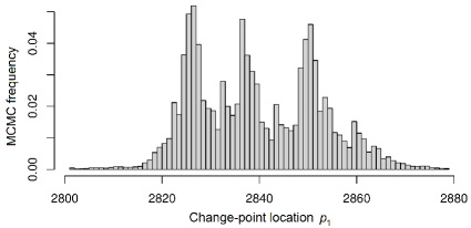
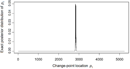
Figure 2: Posterior distribution $\pi(p_{1}|x)$ of the change-point location for the SV40 genome. Left: MCMC histogram of $\pi(p_{1}|x)$ near its mode, after $N=300,000$ MCMC iterations with the first 30,000 samples discarded as burn-in. Right: Entire exact posterior $\pi(p_{1}|x)$.

The MCMC sampler of Section 3.1 was run with $\ell=1$ and $D=10$. The left plot in Figure 2 shows the resulting histogram of the change-point $p_{1}$, between locations 2800 and 2880; there were essentially no MCMC samples outside that interval. Viewing this as an approximation to the posterior $\pi(p_{1}|x)$, the approximate MAP location $\widehat{p}_{1}=2827$ is obtained, which is indeed close to $p_{1}^{*}=2691$.

This result is particularly encouraging, as the BCT-based algorithm used here is a general-purpose method that is agnostic with respect to the nature of the observations – unlike some earlier approaches, it does not utilise any biological information about the structure of the data. Moreover, the value $\widehat{p}_{1}$ is slightly closer to $p_{1}^{*}$ than estimates produced by some of the standard change-point detection methods; e.g., the HMM-based technique in Churchill (1992) gives $\widehat{p}_{1}\approx 2859$, and the Bayesian HMM approach of Totterdell et al. (2017) gives $\widehat{p}_{1}\approx 2854$.

Since this data set is relatively short and contains a single change-point, it is actually possible to compute the entire posterior distribution of the location $p_{1}$ exactly:

$$\pi(p_{1}|x)=\frac{P(x|p_{1})\pi(p_{1}|\ell=1)}{\sum_{p=2}^{n-1}P(x|p)\pi(p|\ell=1)}.$$

Here, $\pi(p_{1}|\ell=1)$ is given by (4), and the terms $P(x|p_{1})$ and $P(x|p)$ in the numerator and denominator can be computed using the CTW algorithm. The resulting exact posterior distribution is shown in the right plot in Figure 2 and in more detail in Figure 3. Even though the shape of the posterior around the mode is quite irregular, the MCMC estimate is almost identical to the true distribution. This indicates that the MCMC sampler converges quite fast and explores all of the support of $\pi(p_{1}|x)$ effectively: The uniform jumps identify the approximate position of the change-point, and the random-walk moves explore the high-probability region around it.

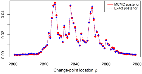
Figure 3: Exact distribution vs. MCMC histogram of $\pi(p_{1}|x)$ for the SV40 genome.

Note that the posterior distribution does not just provide a point estimate for $p_{1}$, but it identifies an interval in which it likely lies, illustrating a common advantage of the Bayesian approach. Also, we should point out that the fact that the posterior here can be computed without resorting to MCMC does not simply indicate that MCMC sampling is sometimes unnecessary. It actually highlights the power of the marginalization provided by the CTW algorithm in that, for relatively short data sets with few change-points, it is possible to get access to the entire exact posterior distribution of interest.

4.2 Unknown number of change-points

4.2.1 Synthetic data

We first examine a synthetic data set of length $n=4300$, generated from four variable-memory chains with values in $A=\{0,1,2\}$. Their models (shown in Figure 4) and associated parameters (given in Appendix B) are chosen to be quite similar, so that the segmentation problem is nontrivial. The locations of the three change-points are $p_{1}^{*}=2500$, $p_{2}^{*}=3500$, $p_{3}^{*}=4000$.

Figure 4: The four tree models used for generating the synthetic data set. The last model is the empty tree consisting of only the root node $\lambda$, corresponding to independent data.

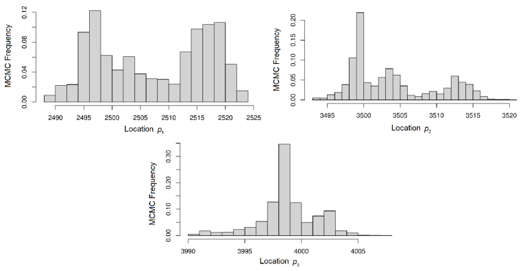
Figure 8: MCMC histograms of the posterior of each change-point location in the simulated data example of Section 4.2.1.

The MCMC sampler of Section 3.2 was run with $\ell_{\text{max}}=10$ and $D=10$. The resulting histogram approximation to the posterior of the number of change-points (left plot in Figure 5) shows that the algorithm identifies the correct value $\ell=3$ with overwhelming confidence. Similarly, the posterior of the change-point locations (right plot in Figure 5) consists of three narrow peaks centered at the true locations. The actual MAP estimates for the change-point locations are $\widehat{p}_{1}=2497$, $\widehat{p}_{2}=3500$, and $\widehat{p}_{3}=3999$. Zoomed-in versions, showing the posterior of the location of each of the three change-points separately are shown in Figure 8 in Appendix C.1.

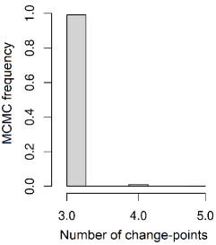
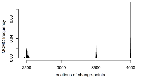
Figure 5: Simulated data. Left: MCMC histogram of the posterior of the number of change-points. Right: MCMC histogram of the posterior of the change-point locations. In both cases,

$N=10^{5}$ MCMC iterations were performed, with the first 10,000 samples discarded as burn-in.

4.2.2 Bacteriophage lambda

Here we revisit the $48,502$ base-pair-long genome of the bacteriophage lambda virus (Sanger et al., 1982), available as sequence NC_001416.1 at the GenBank database (Clark et al., 2016). This data set is often used as a benchmark for comparing different segmentation algorithms (Churchill, 1989, 1992; Braun and Müller, 1998; Braun et al., 2000; Li, 2001; Boys and Henderson, 2004; Gwadera et al., 2008). Due to the high complexity of this genome (which consists of 73 different genes), previous approaches often give different results on both the number and locations of change-points, although all of them have been found to be biologically reasonable. For example, Gwadera et al. (2008) identify a total of 4 change-points, Li (2001); Boys and Henderson (2004) identify 5, Churchill (1992); Braun and Müller (1998) identify 6, and Braun et al. (2000) identify 8 change-points. These differences make it difficult to compare the performance of different methods quantitatively, but judging the biological relevance of the identified segments is still crucial. In order to do so, we will refer to the findings in the standard work of Liu et al. (2013).

The MCMC sampler of Section 3.2 was run with $D=10$ and $\ell_{\text{max}}=10$. The resulting MCMC histogram approximation of the posterior over the number of change-points (Figure 6, left plot) suggests that, with very high probability, there are either $\ell=4$ or $5$ change-points, with $\ell=4$ being over seven times more likely than $\ell=5$.

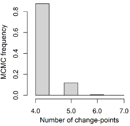
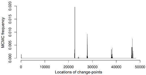
Figure 6: Posterior distribution of the number and location of change-points in the bacteriophage lambda genome. Left: MCMC histogram of the posterior of the number of change-points. Right: MCMC histogram of the posterior of the change-point locations. In both cases, $N=700,000$ MCMC samples were obtained, with the first 70,000 discarded as burn-in.

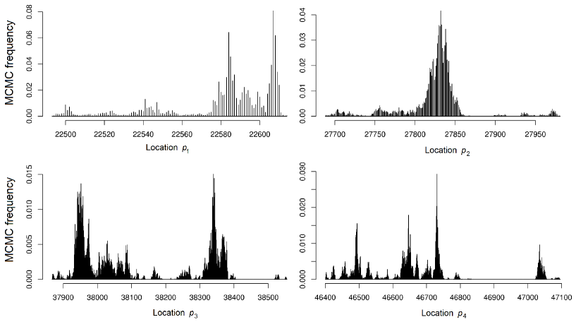
Figure 9: MCMC histograms of the posterior of each change-point location in the bacteriophage lambda genome from Section 4.2.2.

The posterior of the change-point locations (Figure 6, right plot) clearly identifies four significant locations, as well as two more, around positions 100 and 24,000, with significantly smaller weights. Zoomed-in versions, showing the posterior of each of the four main locations are given in Figure 9 in Appendix C.2. The resulting MAP estimates for the change-point locations are shown in Table 1, where they are also compared with the biologically “true” change-points (Liu et al., 2013) and the estimates provided by one of the most reliable, state-of-the-art methods that have been applied to this data (Braun et al., 2000).

Gene	True	BCT	Braun et al. (2000)
ea47	22686	22607	22544
ea59	26973	27832	27829
cro	38315	38340	38029
bor	46752	46731	46528

Table 1: Estimates of change-point locations in the bacteriophage lambda genome.

According to Liu et al. (2013), the segments we identify correspond to a biologically meaningful and important partition in terms of gene expression. The first segment (1-22607) starts at the beginning of the genome and ends very close to the start of gene “ea47” (position $22686$), which signifies the end of the “late operon” and the beginning of the leftward “early operon”, both of which play an important role in transcription. The second segment (22608-27832) essentially consists of the region “b2”, an important region containing the three well-recognized “early” genes “ea47”, “ea31” and “ea59”. The third segment (27833-38340) ends very close to the end of gene “cro” (position $38315$), which is the start of the rightward “early operon” that is also essential in transcription. Lastly, the fourth segment (38341-46731) ends very close to the end (position $46752$) of gene “bor”, one of the major genes being translated.

Compared with previous findings, our results are similar enough to be plausible, while the places where they differ are precisely in the identification of biologically meaningful features, potentially improving performance. Specifically, our estimates are very close to those obtained by Gwadera et al. (2008), where an approach based on variable-memory Markov models is also used: Four change-points are identified by Gwadera et al. (2008), and their estimated locations lie inside the credible regions of our corresponding posteriors.

Compared with the alternative Bayesian approach of Boys and Henderson (2004), the present method gives similar locations and also addresses some of the identified limitations of the Bayesian HMM approach. Firstly, it was seen that the Bayesian HMM framework may be sensitive to the assumed prior distribution on the hidden state transition parameters. In contrast, the present BCT-based framework avoids such problems as it relies on the prior predictive likelihood (which marginalizes over all models and parameters), and uses a simple default value for the only prior hyperparameter, $\beta$. Also, Gupta and Liu (2004) argue that the assumption that all segments share the same memory length may be problematic. The BCT-based methodology requires no such assumptions and, indeed, the MAP tree models obtained by the BCT algorithm in each segment of this data set have maximum depths $d=5,1,2,3$ and $0$, respectively, indicating that the memory length is not constant throughout the genome.

4.2.3 El Niño

El Niño (Trenberth, 1997) is one of the most influential natural climate patterns on earth. It impacts ocean temperatures, the strength of ocean currents, and the local weather in South America. As a result, it has direct societal consequences on areas including the economy (Cashin et al., 2017) and public health (Kovats et al., 2003). Moreover, studying the frequency change of El Niño events can shed light on anthropogenic warming (Timmermann et al., 1999; Cai et al., 2014; Wang et al., 2019). The data set considered here is a binary time series that consists of $495$ annual observations between 1525 to 2020 (Quinn et al., 1987), with 0 representing the absence of an El Niño event and 1 indicating its presence; data for recent years are also available online through the US Climate Prediction Center, at: https://origin.cpc.ncep.noaa.gov/products/analysis_monitoring/ensostuff/ONI_v5.php.

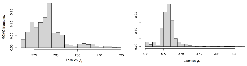
Figure 10: MCMC histograms of the posterior of each change-point location in the meteorological data in Section 4.2.3.

The MCMC sampler of Section 3.2 was run with $D=5$ and $\ell_{\text{max}}=5$. The resulting MCMC estimate of the posterior on the number of change-points (left plot in Figure 7) suggests that the most likely value is $\ell=2$, with $\ell=1$ being a close second. The posterior of the change-point locations (right plot in Figure 7) also shows two clear peaks; zoomed-in versions showing the location of each change-point separately are given in Figure 10 in Appendix C.3.

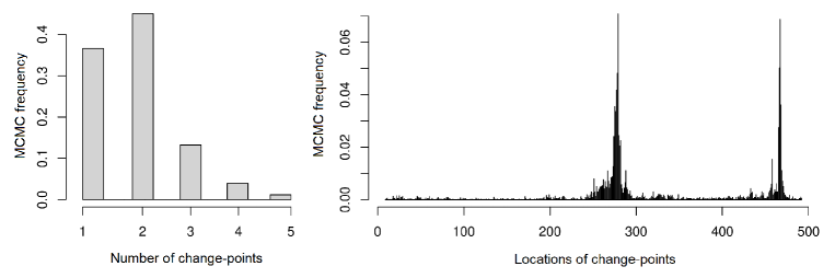
Figure 7: Posterior distribution of the number and location of the change-points for the El Niño data set. Left: MCMC histogram of the posterior of the number of change-points. Right: MCMC histogram of the posterior of the change-point locations. In both cases, $N=20,000$ iterations were performed and the first 2,000 samples were discarded as burn-in.

The MAP estimates of the two locations are at $\widehat{p}_{1}=278$ and $\widehat{p}_{2}=467$, corresponding to historically meaningful events during the years 1802 and 1991, respectively: The first change-point can be attributed to advancements in recording meteorological events, as prior to 1800 only the strong and extreme events were recorded (Quinn et al., 1987). The second change-point in the early 1990s likely indicates a response to greenhouse warming, which is expected to increase both the frequency and the intensity of El Niño events (Cai et al., 2014; Timmermann et al., 1999). Indeed, examining the first-order marginal $\pi=(\pi(0),\pi(1))$ of the stationary distribution associated with the MAP tree model in each segment, we find that the frequency $\pi(1)$ of the recorded El Niño events increases between consecutive segments, from $\pi(1)=0.14$, to $\pi(1)=0.35$, and finally to $\pi(1)=0.54$.

5 Conclusions

A new hierarchical Bayesian framework is developed for modelling time series with change-points as piece-wise homogeneous variable-memory Markov chains, and for the segmentation of corresponding empirical data sets. The proposed framework is based on the BCT class of models and algorithms, and utilises the CTW algorithm to integrate out all models and parameters in each segment. This enables the development of practical and effective MCMC algorithms that can sample directly from the desired posterior distribution of the number and location of the change-points. These MCMC samplers incorporate uniform random jumps that identify the approximate positions of the change-points, as well as short-range random-walk moves that explore the high-probability regions around them. This way, the state space is explored effectively, providing an accurate estimate of the desired posterior distribution.

Compared to earlier techniques, the proposed methodology offers a general and principled Bayesian approach, that achieves very good results without requiring any preliminary information on the nature of the data. Moreover, the proposed Bayesian setting provides a natural quantification of uncertainty for all resulting estimates. In practice, our methods were found to yield results as good as or better than state-of-the-art methods, on both simulated and real-world data sets.

In all our experiments, the proposed approach has found to be very effective for small-sized alphabets, and especially for DNA segmentation problems, which form a key class of crucial applications. An important direction for further work is to consider extensions that would work effectively with large (or continuous) alphabets, particularly in the case of natural language processing problems. Another interesting direction is the development of sequential methods for anomaly detection, in connection with timely questions related to online security.

Appendix

Appendix A MCMC acceptance probability

The ratio $r((\ell,\mbox{\boldmath$p$}),(\ell^{\prime},\mbox{\boldmath$p$}^{\prime}))$ in the acceptance probability of the MCMC sampler in Section 3.2 is given by:

$$\frac{P(x|\boldsymbol{p}^{\prime},\ell^{\prime})}{P(x|\boldsymbol{p},\ell)}\times\frac{{\displaystyle\prod_{j=0}^{\ell^{\prime}}}(p_{j+1}^{\prime}-p_{j}^{\prime}-1)}{{\displaystyle\prod_{j=0}^{\ell}}(p_{j+1}-p_{j}-1)}\times\left\{\begin{array}[]{ll}\frac{2(n-2)}{(n-3)(n-4)},\text{ if }\ell=0;\\ \\ \frac{(n-3)(n-4)}{2(n-2)},\text{ if }\ell=1,\ell^{\prime}=0;\\ \\ \frac{3(2\ell_{\rm max}+1)(n-\ell_{\rm max}-1)}{(n-2\ell_{\rm max}-2)(n-2\ell_{\rm max}-1)},\text{ if }\ell=\ell_{\rm max}-1\text{, }\ell^{\prime}=\ell_{\rm max};\\ \\ \frac{(n-2\ell_{\rm max}-2)(n-2\ell_{\rm max}-1)}{3(2\ell_{\rm max}+1)(n-\ell_{\rm max}-1)},\text{ if }\ell=\ell_{\rm max}\text{, }\ell^{\prime}=\ell_{\rm max}-1;\\ \\ \frac{(n-2\ell-2)(n-2\ell-1)}{2(2\ell+1)(n-\ell-1)},\text{ if }\ell^{\prime}=\ell-1,\;\ell\neq 1,\ell_{\rm max};\\ \\ \frac{2(2\ell^{\prime}+1)(n-\ell^{\prime}-1)}{(n-2\ell^{\prime}-2)(n-2\ell^{\prime}-1)},\text{ if }\ell^{\prime}=\ell+1,\;\ell^{\prime}\neq 1,\ell_{\rm max};\\ \\ 1,\text{ otherwise}.\end{array}\right.$$

Appendix B Parameter values

The parameters of the models generating the simulated data set of Section 4.2.1 are given below.

Model 1	Probability
Context	0	1	2
0	0.3	0.4	0.3
2	0.5	0.3	0.2
10	0.2	0.5	0.3
11	0.1	0.4	0.5
121	0.7	0.2	0.1
122	0.4	0.2	0.4
1200	0.6	0.1	0.3
1201	0.3	0.5	0.2
1202	0.4	0.1	0.5

Model 2	Probability
Context	0	1	2
0	0.4	0.5	0.1
2	0.4	0.4	0.2
10	0.4	0.2	0.4
11	0.2	0.4	0.4
12	0.6	0.1	0.3

Model 3	Probability
Context	0	1	2
0	0.5	0.3	0.2
1	0.3	0.6	0.1
2	0.3	0.2	0.5
Model 4	Probability
Context	0	1	2
$\lambda$	0.4	0.2	0.4

Appendix C Additional results

C.1 Synthetic data

C.2 Bacteriophage lambda genome

C.3 El Niño event data

References

- Aminikhanghahi and Cook [2017] S. Aminikhanghahi and D. Cook. A survey of methods for time series change point detection. Knowl. Inf. Syst., 51(2):339–367, September 2017.
- Boys and Henderson [2004] R.J. Boys and D.A. Henderson. A Bayesian approach to DNA sequence segmentation. Biometrics, 60(3):573–581, September 2004.
- Braun and Müller [1998] J.V. Braun and H.G. Müller. Statistical methods for DNA sequence segmentation. Statist. Sci., 13(2):142–162, 1998.
- Braun et al. [2000] J.V. Braun, R.K. Braun, and H.G. Müller. Multiple changepoint fitting via quasilikelihood, with application to DNA sequence segmentation. Biometrika, 87(2):301–314, 2000.
- Bühlmann and Wyner [1999] P. Bühlmann and A.J. Wyner. Variable length Markov chains. Ann. Statist., 27(2):480–513, April 1999.
- Cai et al. [2014] W. Cai, S. Borlace, M. Lengaigne, P. Rensch, M. Collins, G. Vecchi, A. Timmermann, A. Santoso, M. McPhaden, L. Wu, M. England, G. Wang, E. Guilyardi, and F.F. Jin. Increasing frequency of extreme El Niño events due to greenhouse warming. Nature Climate Change, 4(2):111–116, 2014.
- Cashin et al. [2017] P. Cashin, K. Mohaddes, and M. Raissi. Fair weather or foul? The macroeconomic effects of El Niño. Journal of International Economics, 106(C):37–54, 2017.
- Chandola et al. [2012] V. Chandola, A. Banerjee, and V. Kumar. Anomaly detection for discrete sequences: A survey. IEEE Transactions on Knowledge and Data Engineering, 24(5):823–839, May 2012.
- Churchill [1989] G.A. Churchill. Stochastic models for heterogeneous DNA sequences. Bulletin of Mathematical Biology, 51(1):79–94, 1989.
- Churchill [1992] G.A. Churchill. Hidden Markov chains and the analysis of genome structure. Computers & Chemistry, 16(2):107–115, 1992.
- Clark et al. [2016] K. Clark, I. Karsch-Mizrachi, D.J. Lipman, J. Ostell, and E.W. Sayers. GenBank. Nucleic Acids Research, 44(D1):D67–D72, January 2016. Online at: www.ncbi.nlm.nih.gov.
- Fearnhead [2006] P. Fearnhead. Exact and efficient Bayesian inference for multiple changepoint problems. Stat. Comput., 16(2):203–213, 2006.
- Green [1995] P.J. Green. Reversible jump Markov chain Monte Carlo computation and Bayesian model determination. Biometrika, 82(4):711–732, December 1995.
- Gupta and Liu [2004] M. Gupta and J.S. Liu. Discussion of “A Bayesian approach to DNA sequence segmentation”. Biometrics, 60(3):582–583, 2004.
- Gwadera et al. [2008] R. Gwadera, A. Gionis, and H. Mannila. Optimal segmentation using tree models. Knowl. Inf. Syst., 15(3):259–283, May 2008.
- Jacob and Bansal [2008] T. Jacob and R.K. Bansal. Sequential change detection based on universal compression algorithms. In 2008 IEEE International Symposium on Information Theory (ISIT), pages 1108–1112, Toronto, ON, July 2008.
- Juvvadi and Bansal [2013] D.R. Juvvadi and R.K. Bansal. Sequential change detection using estimators of entropy & divergence rate. In 2013 National Conference on Communications (NCC), pages 1–5, New Delhi, India, March 2013.
- Kass and Raftery [1995] R.E. Kass and A.E. Raftery. Bayes factors. J. Amer. Statist. Assoc., 90(430):773–795, 1995.
- Kehagias [2004] A. Kehagias. A hidden Markov model segmentation procedure for hydrological and environmental time series. Stochastic Environmental Research and Risk Assessment, 18(2):117–130, April 2004.
- Kontoyiannis et al. [2021] I. Kontoyiannis, L. Mertzanis, A. Panotonoulou, I. Papageorgiou, and M. Skoularidou. Revisiting context-tree weighting for Bayesian inference. In 2021 IEEE International Symposium on Information Theory (ISIT), pages 2906–2911, Melbourne, Australia, July 2021.
- Kontoyiannis et al. [2022] I. Kontoyiannis, L. Mertzanis, A. Panotonoulou, I. Papageorgiou, and M. Skoularidou. Bayesian Context Trees: Modelling and exact inference for discrete time series. To appear, Journal of the Royal Statistical Society: Series B, also at arXiv 2007.14900 [stat.ME], 2022.
- Koolen and de Rooij [2013] W.M. Koolen and S. de Rooij. Universal codes from switching strategies. IEEE Trans. Inform. Theory, 59(11):7168–7185, 2013.
- Kovats et al. [2003] S. Kovats, M. Bouma, S. Hajat, E. Worrall, and A. Haines. El Niño and health. Lancet, 362(9394):1481–1489, 2003.
- Li [2001] W. Li. DNA segmentation as a model selection process. In Proceedings of the Fifth Annual International Conference on Computational Biology, pages 204–210, Montreal, Quebec, April 2001.
- Liu et al. [2013] X. Liu, H. Jiang, Z. Gu, and J.W. Roberts. High-resolution view of bacteriophage lambda gene expression by ribosome profiling. Proceedings of the National Academy of Sciences, 110(29):11928–11933, 2013.
- Mächler and Bühlmann [2004] M. Mächler and P. Bühlmann. Variable length Markov chains: Methodology, computing, and software. J. Comput. Grap. Stat., 13(2):435–455, 2004.
- Merhav [1993] N. Merhav. On the minimum description length principle for sources with piecewise constant parameters. IEEE Trans. Inform. Theory, 39(6):1962–1967, November 1993.
- Merhav and Feder [1995] N. Merhav and M. Feder. A strong version of the redundancy-capacity theorem of universal coding. IEEE Trans. Inform. Theory, 41(3):714–722, May 1995.
- Papageorgiou and Kontoyiannis [2021] I. Papageorgiou and I. Kontoyiannis. Hierarchical Bayesian mixture models for time series using context trees as state space partitions. arXiv e-prints, 2106.03023 [stat.ME], June 2021.
- Papageorgiou and Kontoyiannis [2022] I. Papageorgiou and I. Kontoyiannis. Posterior representations for bayesian Context Trees: Sampling, estimation and convergence. arXiv e-prints, 2022.02230 [math.ST], July 2022.
- [31] I. Papageorgiou, V.M. Lungu, and I. Kontoyiannis. BCT: Bayesian Context Trees for discrete time series. R package version 1.1, December 2020; version 1.2, May 2022. Availble online at: CRAN.R-project.org/package=BCT.
- Quinn et al. [1987] W.H. Quinn, V.T. Neal, and S.E. Antunez De Mayolo. El Niño occurrences over the past four and a half centuries. Journal of Geophysical Research: Oceans, 92(C13):14449–14461, 1987.
- Rasmussen and Ghahramani [2000] C. Rasmussen and Z. Ghahramani. Occam’s razor. Advances in Neural Information Processing Systems, 13, 2000.
- Reddy et al. [1978] V.B. Reddy, B. Thimmappaya, R. Dhar, K.N. Subramanian, B.S. Zain, J. Pan, P.K. Ghosh, M.L. Celma, and S.M. Weissman. The genome of Simian virus 40. Science, 200(4341):494–502, 1978.
- Rissanen [1983a] J. Rissanen. A universal prior for integers and estimation by minimum description length. Ann. Statist., 11(2):416–431, June 1983a.
- Rissanen [1983b] J. Rissanen. A universal data compression system. IEEE Trans. Inform. Theory, 29(5):656–664, September 1983b.
- Rissanen [1986] J. Rissanen. Complexity of strings in the class of Markov sources. IEEE Trans. Inform. Theory, 32(4):526–532, July 1986.
- Rissanen [1987] J. Rissanen. Stochastic complexity. Journal of the Royal Statistical Society: Series B, 49(3):223–239, 253–265, 1987. With discussion.
- Robert and Casella [2004] C.P. Robert and G. Casella. Monte Carlo statistical methods. Springer-Verlag, New York, second edition, 2004.
- Rotondo et al. [2019] J.C. Rotondo, E. Mazzoni, I. Bononi, M. Tognon, and F. Martini. Association between Simian virus 40 and human tumors. Frontiers in Oncology, 9:670, 2019.
- Sanger et al. [1982] F. Sanger, A.R. Coulson, G.F. Hong, D.F. Hill, and G.B. Petersen. Nucleotide sequence of bacteriophage DNA. Journal of Molecular Biology, 162(4):729–773, 1982.
- Schwarz [1978] G. Schwarz. Estimating the dimension of a model. Ann. Statist., 6(2):461–464, March 1978.
- Shamir [2003] G.I. Shamir. On strongly sequential compression of sources with abrupt changes in statistics. In 2003 IEEE International Conference on Communications (ICC), volume 4, pages 2924–2927, Anchorage, AK, May 2003.
- Shamir and Costello [2000] G.I. Shamir and D.J. Costello. Asymptotically optimal low-complexity sequential lossless coding for piecewise-stationary memoryless sources. I. The regular case. IEEE Trans. Inform. Theory, 46(7):2444–2467, November 2000.
- Shamir and Costello [2001] G.I. Shamir and D.J. Costello. On the redundancy of universal lossless coding for general piecewise stationary sources. Communications in Information and Systems, 1(7):305–332, Januray 2001.
- Shamir and Merhav [1999] G.I. Shamir and N. Merhav. Low-complexity sequential lossless coding for piecewise-stationary memoryless sources. IEEE Trans. Inform. Theory, 45(5):1498–1519, July 1999.
- Shimada et al. [2021] K. Shimada, S. Saito, and T. Matsushima. An efficient Bayes coding algorithm for the non-stationary source in which context tree model varies from interval to interval. In 2021 IEEE Information Theory Workshop (ITW), pages 1–6, Kanazawa, Japan, October 2021.
- Smith and Spiegelhalter [1980] A.F.M. Smith and D.J. Spiegelhalter. Bayes factors and choice criteria for linear models. Journal of the Royal Statistical Society: Series B, 42(2):213–220, 1980.
- Timmermann et al. [1999] A. Timmermann, J.M. Oberhuber, A. Bacher, M. Esch, M. Latif, and E. Roeckner. Increased El Niño frequency in a climate model forced by future greenhouse warming. Nature, 398(6729):694–697, 1999.
- Totterdell et al. [2017] J.A. Totterdell, D. Nur, and K.L. Mengersen. Bayesian hidden Markov models in DNA sequence segmentation using R: The case of simian vacuolating virus (SV40). Journal of Statistical Computation and Simulation, 87(14):2799–2827, 2017.
- Trenberth [1997] K.E. Trenberth. The definition of El Niño. Bulletin of the American Meteorological Society, 78(12):2771–2778, 1997.
- Truong et al. [2020] C. Truong, L. Oudre, and N. Vayatis. Selective review of offline change point detection methods. Signal Processing, 176:107299, February 2020.
- van den Burg and Williams [2020] G.J.J. van den Burg and C.K.I. Williams. An evaluation of change point detection algorithms. arXiv e-prints, [2007.14900 stat.ML], March 2020.
- Veness et al. [2012] J. Veness, K.S. Ng, M. Hutter, and M.H. Bowling. Context tree switching. In 2012 Data Compression Conference, pages 327–0336, April 2012.
- Veness et al. [2013] J. Veness, M. White, M. Bowling, and A. György. Partition tree weighting. In 2013 Data Compression Conference, pages 321–330, March 2013.
- Verma and Bansal [2019] A. Verma and R.K. Bansal. Sequential change detection based on universal compression for Markov sources. In 2019 IEEE International Symposium on Information Theory (ISIT), pages 2189–2193, Paris, France, July 2019.
- Wang et al. [2019] B. Wang, X. Luo, Y.M. Yang, W. Sun, M.A. Cane, W. Cai, S.W. Yeh, and J. Liu. Historical change of El Niño properties sheds light on future changes of extreme El Niño. Proceedings of the National Academy of Sciences, 116(45):22512–22517, 2019.
- Willems [1996] F.M.J. Willems. Coding for a binary independent piecewise-identically-distributed source. IEEE Trans. Inform. Theory, 42(6):2210–2217, November 1996.
- Willems [1998] F.M.J. Willems. The context-tree weighting method: Extensions. IEEE Trans. Inform. Theory, 44(2):792–798, March 1998.
- Willems et al. [1995] F.M.J. Willems, Y.M. Shtarkov, and T.J. Tjalkens. The context tree weighting method: Basic properties. IEEE Trans. Inform. Theory, 41(3):653–664, May 1995.
- Yamanishi and Fukushima [2018] K. Yamanishi and S. Fukushima. Model change detection with the MDL principle. IEEE Trans. Inform. Theory, 64(9):6115–6126, September 2018.