TOI-1670 b and c: An Inner Sub-Neptune with an Outer Warm Jupiter
Unlikely to have Originated from High-Eccentricity Migration

Abstract

We report the discovery of two transiting planets around the bright ($V=9.9$ mag) main sequence F7 star TOI-1670 by the Transiting Exoplanet Survey Satellite. TOI-1670 b is a sub-Neptune ($R_{\mathrm{b}}=2.06_{-0.15}^{+0.19}$ $R_{\earth}$) on a 10.9-day orbit and TOI-1670 c is a warm Jupiter ($R_{\mathrm{c}}=0.987_{-0.025}^{+0.025}$ $R_{\mathrm{Jup}}$) on a 40.7-day orbit. Using radial velocity observations gathered with the Tull coudé Spectrograph on the Harlan J. Smith telescope and HARPS-N on the Telescopio Nazionale Galileo, we find a planet mass of $M_{\mathrm{c}}=0.63_{-0.08}^{+0.09}$ $M_{\mathrm{Jup}}$ for the outer warm Jupiter, implying a mean density of $\rho_{c}=0.81_{-0.11}^{+0.13}$ g cm^-3. The inner sub-Neptune is undetected in our radial velocity data ($M_{\mathrm{b}}<0.13$ $M_{\mathrm{Jup}}$ at the 99% confidence level). Multi-planet systems like TOI-1670 hosting an outer warm Jupiter on a nearly circular orbit ($e_{\mathrm{c}}=0.09_{-0.04}^{+0.05}$) and one or more inner coplanar planets are more consistent with “gentle” formation mechanisms such as disk migration or in situ formation rather than high-eccentricity migration. Of the 11 known systems with a warm Jupiter and a smaller inner companion, 8 (73%) are near a low-order mean-motion resonance, which can be a signature of migration. TOI-1670 joins two other systems (27% of this subsample) with period commensurabilities greater than 3, a common feature of in situ formation or halted inward migration. TOI-1670 and the handful of similar systems support a diversity of formation pathways for warm Jupiters.

1 Introduction

The origin of giant planets interior to the water ice line remains an open question. A number of theories have been proposed to explain the closest-in ($P<10$ d) giant planets, or hot Jupiters (HJs; e.g., Dawson & Johnson 2018; Fortney et al. 2021). These scenarios are primarily divided between dynamically “violent” or “gentle” mechanisms. The former consists of three-body dynamical interactions such as planet-planet scattering or high-eccentricity tidal migration (e.g., Wu & Murray 2003; Fabrycky & Tremaine 2007; Triaud et al. 2010; Naoz et al. 2011; Batygin 2012). The latter refers to disk migration (e.g., Ward 1997; Albrecht et al. 2012; Kley & Nelson 2012) or in situ formation (e.g., Boley et al. 2016; Huang et al. 2016; Batygin et al. 2016; Anderson et al. 2020). These processes have also been used to explain part of the farther-out population of warm Jupiters (WJs; defined here to have $10<P<200$ d). However, observed WJ demographics suggest that multiple processes are present in sculpting these more distant giant systems.

WJs can be broadly divided into two classes. The first is a transient population that will likely evolve into HJs. In more disruptive formation mechanisms such as high-eccentricity tidal migration, giant planets at comparatively wide separations are disturbed onto highly eccentric orbits by a third body via planet-planet scattering or Von Zeipel–Lidov–Kozai oscillations and eventually circularize into orbits with shorter periods (Lidov 1962; Kozai 1962; Naoz 2016; Ito & Ohtsuka 2019). Eccentric giant planets undergoing this tidally damped inward migration are caught in a rapid, temporary state (Naef et al. 2001; Dawson & Johnson 2018; Dong et al. 2021; Jackson et al. 2021). They are expected to start their journeys with much higher eccentricities ($e\gtrsim 0.9$; Vick et al. 2019) which can decay as rapidly as $\sim$1 Myr as they settle in near their host star (Patra et al. 2020; Mancini et al. 2021). The majority of WJs are not expected to belong to this transient classification.

Instead, most WJs are a part of a “static” population that will remain stable over long time periods. This group consists of the apparently single systems with low to moderate eccentricities as well as co-planar multi-planet systems containing WJs with low eccentricities. These WJs have periapses larger than what is required for efficient tidal damping of their orbits, which occurs at $\lesssim$0.05 AU (Anderson et al. 2016; Dong et al. 2021), so these planets cannot be undergoing high-eccentricity migration. If most giant planets form beyond the water ice line, other migration mechanisms must play a major role in sculpting these WJ orbital properties and demographics (e.g., Veras & Armitage 2005; Fogg & Nelson 2009; Dong et al. 2014; Ortiz et al. 2015; Huang et al. 2016; Anderson & Lai 2017; Anderson et al. 2020; Schlecker et al. 2020). However, the relative importance of these pathways is still unknown. Investigating WJ orbital eccentricities can place additional constraints on the dominant giant planet migration mechanism since each scenario will produce different observed eccentricity distributions.

Warm Jupiters have an eccentricity distribution that peaks at $e=0.0$ with a tail that extends out to $e\sim 0.8$ (Kipping 2013; Dong et al. 2021). In order to produce the population of WJs with moderately eccentric orbits ($e\sim 0.2-0.7$), a mechanism is needed that can excite eccentricities. These potential excitation scenarios include interactions involving a disk (e.g., Goldreich & Sari 2003; Petrovich et al. 2019), secular eccentricity oscillations driven by interactions with a distant inclined giant planet (e.g., Anderson & Lai 2017), and planet-planet scattering events (e.g., Mustill et al. 2017; Frelikh et al. 2019; Marzari & Nagasawa 2019; Anderson et al. 2020). An important clue is the observed dependence on metallicity of the giant planet eccentricity distribution, where metal-rich systems (that may more favorably form multiple giant planets) are more likely to host eccentric gas giants (Dawson & Murray-Clay 2013).

Systems hosting WJs with low-mass inner companions on coplanar orbits are especially useful laboratories to test these planet formation and migration theories. Their small orbital eccentricities and low mutual inclinations suggest that disk migration or in situ formation likely helped create this population. WJs have a relatively high close companion rate of nearly 50% (Huang et al. 2016). However, their intrinsically low occurrence rate ($\sim$1–2%; Cumming et al. 2008) combined with the difficulty of detecting lower-mass inner planets means that only a handful of known multi-planet systems host a WJ (Johnson et al. 2010; Santerne et al. 2016; Fernandes et al. 2019). Increasing the number of systems with this multi-planet architecture may further distinguish this subsample into two WJ populations, each of which likely reflects different formation and migration routes.

Here we present the discovery of the transiting multi-planet system TOI-1670 bc, a warm Jupiter (TOI-1670 c) with an inner sub-Neptune (TOI-1670 b) found with the Transiting Exoplanet Survey Satellite (TESS; Ricker et al. 2015). TOI-1670 b and c were originally identified by the TESS Science Processing Operations Center (SPOC; Jenkins et al. 2016) pipeline as two promising transiting signals that were subsequently promoted to TESS Object of Interest (TOI; Guerrero et al. 2021) status. TOI-1670 (TIC ID 441739020; 2MASS J17160415+7209402; Gaia DR2 1651911084230149248) is a relatively inactive (log$R^{\prime}_{\mathrm{HK}}=-4.93$) old F7 dwarf with a TESS apparent magnitude of 9.5 mag and a moderate projected rotational velocity of $\approx$9 km s^-1 (see Section 3). In this work, we validate both planets and measure the mass of the outer planet TOI-1670 c. In Section 2, we describe the TESS photometric data and follow-up radial velocity (RV) observations used in the planet validation and mass measurement. Our characterization of the system, including the host star and a global fit to the RVs and light curve, is presented in Section 3. We conclude in Section 4 by contextualizing TOI-1670 in the paradigm of WJs and their formation.

2 Observations

KESPRINT is an international collaboration focused on the discovery, confirmation, and characterization of exoplanet candidates from space-based missions (e.g., Persson et al. 2018; Gandolfi et al. 2018; Livingston et al. 2019; Lam et al. 2020; Šubjak et al. 2020). As part of this consortium, a series of ground-based follow-up observations of TOI-1670 were taken. These data are primarily used to reject the possibility of a false positive scenario in which the observed transiting signal is caused by something other than a planet. For example, this includes a low-mass eclipsing binary (EB), a grazing transit of an EB, a background EB, or a transiting planet around a background star. Reconnaissance spectra are used to exclude an EB scenario by constraining the maximum amplitude of the RV signal. High-resolution speckle images are taken to exclude binary companions to TOI-1670 and nearby background stars. High-resolution spectra are used to characterize the host star and, when possible, measure the masses of the planets.

2.1 TESS Photometry

TOI-1670 was observed by TESS at 2-minute cadence over 11 sectors (15, 16, 18, 19, 20, 21, 22, 23, 24, 25, and 26) for a total of 323 days. Images were reduced and light curves were analyzed for transit signals with the TESS SPOC pipeline (Jenkins et al. 2016), which identified two potential transit signals (Jenkins 2002; Jenkins et al. 2010, 2020) with periods of 40.7 days (TOI 1670.01) and 10.9 days (TOI 1670.02). SPOC vetting tests (Twicken et al. 2018; Li et al. 2019) validated both signals as consistent with planets and they were designated as TOIs (Guerrero et al. 2021) by the TESS Science Office.

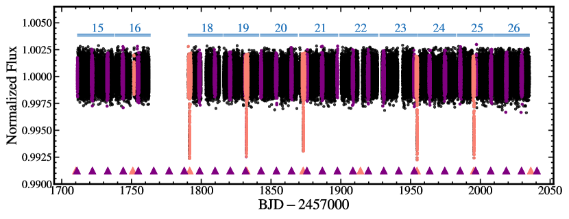
Figure 1: The detrended TESS light curve of TOI-1670. The full light curve is shown in black. Colored purple and pink points are relative photometry within four transit duration before and after transits of TOI-1670 b and c, respectively, and are used in the global RV and light curve model fit. Times of transit are also marked by triangles plotted along the time axis. Gaps in the light curve correspond to periods where TESS uploaded data, result from data quality cuts, or are during Sector 17 when TOI-1670 was not observed. TESS sectors are shown in blue above the light curve.

We downloaded the SPOC Pre-search Data Conditioning Simple Aperture Photometry (PDCSAP) light curve (Smith et al. 2012; Stumpe et al. 2012, 2014) from the MAST data archive using the lightkurve (Lightkurve Collaboration et al. 2018) software package. We removed all of the photometric measurements that are flagged as poor quality by the SPOC pipeline (DQUALITY > 0) or where either the flux or flux error is listed as NaN. Outlier rejection was performed at 3$\sigma$ for positive outliers and 10$\sigma$ for negative outliers to allow for transit events. The lightcurve is flattened by removing low frequency trends using a Savitzky-Golay filter (Savitzky & Golay 1964) after all transit events were masked out. The final light curve for TOI-1670 is shown in Figure 1. Photometric points used in the global model fit are colored purple and pink. These cover the transit events for TOI-1670 b and c, respectively, and their times of transit are further denoted by the corresponding colored triangles along the time axis.

2.2 TRES Reconnaissance Spectroscopy

We obtained six spectra of TOI-1670 with the Tillinghast Reflector Échelle Spectrograph (TRES; Fűrész 2008) on the 1.5-meter Tillinghast telescope at the Fred L. Whipple Observatory on UT 2020 February 2 and 20, UT 2020 March 6, 9, and 16, and UT 2020 July 7. Exposure times range from 300 to 650 seconds and have an average S/N of $32\pm 5$. Radial velocities were extracted following Buchhave et al. (2010a). Spectra have an average measurement error of 53 m s^-1 and an RMS of 54 m s^-1, which exclude the possibility of an eclipsing binary scenario; however these spectra are not used as part of the orbit fit. Table 6 in Appendix A reports the RV measurements.

2.3 OES Reconnaissance Spectroscopy

We collected 32 spectra using the Ondřejov Échelle Spectrograph (OES) on the 2-meter Perek telescope at the Ondřejov Observatory in the Czech Republic (Kabáth et al. 2020). These observations were obtained between UT 2020 February and UT 2020 September at a cadence of $3-5$ RVs per month. We extracted the spectra and performed the bias, flat-field, and cosmic ray corrections using standard IRAF 2.16 routines (Tody 1993). RVs were extracted using the IRAF cross correlation fxcor taking the highest S/N spectrum as a template. The average measurement error is 110 m s^-1 and the RV RMS is 116 m s^-1. The Doppler signals for TOI-1670 b and c are not detected in this dataset so they are not used in the orbit fit. However, they are used to reject an eclipsing binary scenario and justified further follow-up of TOI-1670 with precise RV measurements. The reconnaissance RV measurements are reported in Table 6 in Appendix A.

2.4 Tull coudé Spectroscopy

We used the Tull coudé Spectrograph on the 2.7-m Harlan J. Smith telescope at McDonald Observatory to obtain 49 spectra of TOI-1670 between UT 2020 April and UT 2021 September. The Tull coudé Spectrograph is a cross-dispersed échelle spectrograph with a wavelength coverage ranging from 3750 $\AA$ to 10200 $\AA$ (Tull et al. 1995). Our configuration uses a $1.2\arcsec{}$ slit which yields a resolving power of $R=$ 60,000. Precise wavelength calibration and instrumental profile reconstruction is achieved with a temperature-controlled iodine vapor (I₂) cell that is mounted in front of the entrance slit.

Radial velocities are extracted using the RV reduction pipeline Austral (Endl et al. 2000). The I₂ cell imprints a well-understood reference absorption spectrum onto the stellar spectra. Precise differential radial velocities are then calculated by comparing each stellar-plus-iodine spectrum with a high S/N stellar template devoid of iodine lines. The S-index activity metric for each spectrum is also calculated and calibrated onto the Mt. Wilson S-index system following the description in Paulson et al. (2002). Table 7 in Appendix A reports the resulting RVs, activity indices, and related measurement errors.

2.5 FIES Spectroscopy

We acquired 7 spectra of TOI-1670 using the Fibre-fed Échelle Spectrograph (FIES; Frandsen & Lindberg 1999; Telting et al. 2014) at the 2.56-m Nordic Optical Telescope (NOT; Djupvik & Andersen 2010) of Roque de los Muchachos Observatory (La Palma, Spain). The observations were carried out between UT 2020 May 25 and UT 2020 September 6 as part of the Spanish CAT observing program 59-210. We used the FIES high-resolution mode, which provides a resolving power of $R=$ 67,000 in the spectral range $3760-8220$ $\AA$. We traced the RV drift of the instrument by acquiring long-exposed ThAr spectra (exposure time of 90 seconds) immediately before and after each science observation. The science exposure time was set to $1200-1800$ seconds, depending on the sky conditions and scheduling constraints. The data reduction follows the steps described in Buchhave et al. (2010b) and Gandolfi et al. (2015) and includes bias subtraction, flat fielding, order tracing and extraction, and wavelength calibration. Radial velocities were derived via multi-order cross-correlations, using the first stellar spectrum as a template. The SNR per pixel at 5500 Å ranges between 40 and 65. The average RV uncertainty is $13.4\pm 2.4$ m s^-1.

2.6 HARPS-N Spectroscopy

We observed TOI-1670 with the HARPS-N spectrograph ($R\approx$ 115,000) on the 3.59-m Telescopio Nazionale Galileo (TNG) at Roque de los Muchachos Observatory located in La Palma, Spain between UT 2020 August and UT 2020 September (Cosentino et al. 2012, 2014) during observing program A40TAC_22 (PI: Gandolfi). A total of 8 spectra were taken; seven spectra had an exposure time of 1800 seconds and one had an exposure time of 215 seconds. This resulted in an average S/N at 550 nm of $84\pm 16$ for the first seven spectra and a S/N of 15 for the shorter exposure.

We used the standard HARPS-N Data Reduction Software (DRS) with a G2 numerical mask to extract the RVs (Pepe et al. 2002). The RVs, their measurement errors, and associated activity indicators such as the bisector inverse slope (BIS), FWHM of the cross-correlation function (CCF), and S-index produced by the HARPS-N DRS are listed in Table 7 of Appendix A.

2.7 High-resolution Imaging

On the nights of UT 2021 April 5 and June 24, TOI-1670 was observed with the NESSI and ‘Alopeke speckle imagers (Scott et al. 2018; Scott 2019), mounted on the 3.5-m WIYN telescope at Kitt Peak and the 8.1-m Gemini North telescope on Mauna Kea, respectively. Both instruments simultaneously acquire data in two bands centered at 562 nm and 832 nm using high speed electron-multiplying CCDs (EMCCDs). Observations of TOI-1670 were performed in the 562 nm and 832 nm bands following the procedures described in Howell et al. (2011). The resulting reconstructed images have a 5$\sigma$ delta magnitude contrast of 4 to 8 magnitudes at angular separations from 20 mas to 1.2″ in the 832 nm band (Figure 2). No other companion sources are detected in the reconstructed images within these angular limits down to the contrasts obtained. These angular limits correspond to spatial separations of 3.3 to 200 AU at the distance of TOI-1670.

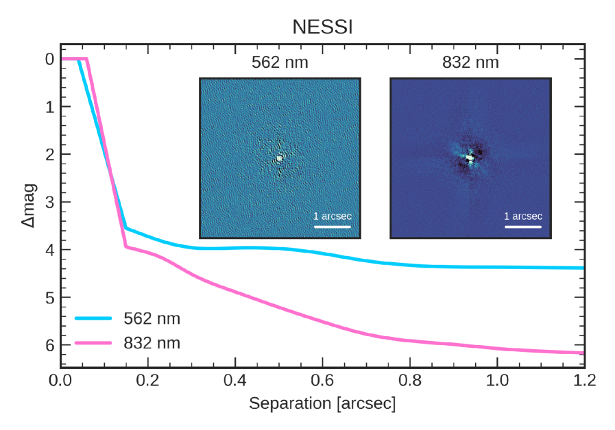
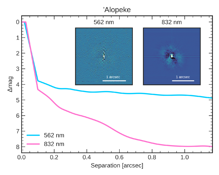
Figure 2: Reconstructed speckle images of TOI-1670 from NESSI (top) and ‘Alopeke (bottom) in the 562 nm and 832 nm bands and their corresponding $5\sigma$ contrast curves. North is up and east is to the left.

3 Analysis

3.1 Stellar Parameters

Planetary parameters measured from the global joint fit of the transit and RV data depend on precise stellar mass and radius measurements. In particular, $R_{p}$ is determined from the transit depth and $M_{p}$ from the RV semi-amplitude, which are dependent on $R_{*}$ and $M_{*}$, respectively. The stellar mass and radius can be inferred with atmospheric and evolutionary models using the spectroscopic parameters ($T_{\mathrm{eff}}$, log$g$, [Fe/H], $v$sin$i$). We determine both these spectroscopic and fundamental parameters for TOI-1670 using several approaches described below.

3.1.1 Spectral Analysis

We analyzed the co-added HARPS-N (S/N = 180) spectrum with the spectral analysis package Spectroscopy Made Easy (SME; Valenti & Piskunov 1996; Valenti & Fischer 2005; Piskunov & Valenti 2017). SME’s spectral fitting technique minimizes the $\chi^{2}$ value by fitting synthetic spectra of stars based on grids of atmosphere models and observations. We fit the co-added HARPS-N spectrum with the ATLAS12 model spectra (Kurucz 2013) using the non-local thermodynamic equilibrium (non-LTE) SME version 5.2.2 following the procedure described in Fridlund et al. (2017) to compute $T_{\mathrm{eff}}$, log$g$, $v$sin$i$, and chemical abundances. The stellar surface gravity, log$g$, was estimated using the spectral wings of the Ca i 6102, 6122, 6162 Å triplet and the Ca i 6439 Å line. The microscopic and macroscopic turbulences, $V_{\mathrm{mic}}$ and $V_{\mathrm{mac}}$, were held fixed to the values determined in the calibration for stars with similar $T_{\mathrm{eff}}$ and log$g$ from Bruntt et al. (2010) and Doyle et al. (2014), respectively.

We also derive the stellar parameters using the publicly available SpecMatch-Emp software package (Yee et al. 2017). SpecMatch-Emp compares the HARPS-N template spectrum to a high resolution ($R\sim 55000$), high S/N ($>$100) Keck/HIRES optical spectral library of 404 well-characterized early- to late-type dwarfs (F1 to M5). The empirical spectra are calibrated using interferometry so SpecMatch-Emp produces estimates for $T_{\mathrm{eff}}$, [Fe/H], and $R_{*}$ (instead of log$g$). Prior to running the code, we convert the HARPS-N spectrum template onto the Keck/HIRES format following the procedure described in Hirano et al. (2018).

The stellar parameters derived from SME and SpecMatch-Emp are in good agreement with each other (Table 1). From SME, we find an effective temperature of $T_{\mathrm{eff}}=6170\pm 61$ K and metallicity of [Fe/H] = 0.09 $\pm$ 0.07 dex, while SpecMatch-Emp gives $T_{\mathrm{eff}}=6048\pm 110$ K and [Fe/H] $=0.05\pm 0.09$ dex; these are consistent with each other within 1$\sigma$. These results are also in good agreement with the photometrically derived effective temperature from Gaia DR2 ($T_{\mathrm{eff}}=6162_{-175}^{+162}$ K) and agree at the 2$\sigma$ level with the TESS Input Catalog (TIC) v8 (Guerrero et al. 2021) value of $6345\pm 121$ K. For this work, we adopt the spectroscopic parameters from SME as it produces all atmospheric parameters. The final adopted stellar parameters are reported in Section 3.1.2.

Table 1: Spectroscopic parameters of TOI-1670 derived using SME and SpecMatch-Emp.

Method	$T_{\mathrm{eff}}$ (K)	log$g$ (g cm-3)	[Fe/H] (dex)	$v$sin$i$ (km s-1)
SME	$6170\pm 61$	$4.29\pm 0.11$	$0.09\pm 0.07$	$9.2\pm 0.6$
SpecMatch-Emp	$6048\pm 110$	$\cdots$	$0.05\pm 0.09$	$\cdots$

3.1.2 Stellar Mass and Radius

We infer the stellar radius by fitting the spectral energy distribution (SED) of TOI-1670 using the software package ARIADNE. ARIADNE utilizes a Bayesian Model Averaging (BMA) framework that convolves four stellar atmosphere models—Phoenix v2 (Husser et al. 2013), BT-Settl (Allard et al. 2011), Kurucz (1993), and Castelli & Kurucz (2003)—with the response functions of commonly available broadband filters. For our SED fitting, we use the 2MASS $JHK_{s}$, Gaia DR2 ($G$, $G_{\mathrm{BP}}$, $B_{\mathrm{RP}}$), Johnson $V$ and $B$, and WISE ($W1$ and $W2$) bandpasses. Synthetic SEDs are created by interpolating in $T_{\mathrm{eff}}$–$\mathrm{log}g$–$\mathrm{[Fe/H]}$ space. Distance, radius, $A_{V}$, and excess photometric uncertainty terms are free parameters in the fitting process. We set the priors for $T_{\mathrm{eff}}$, log$g$, and [Fe/H] to the values we found in Section 3.1.1; the distance prior to the Bailer-Jones et al. (2021) Bayesian-based value ($165.72^{+0.32}_{-0.38}$ pc); and the stellar radius prior to the Gaia DR2 value ($R_{*}=1.38^{+0.08}_{-0.07}$ $R_{\odot}$). The extinction, $A_{V}$, has a flat prior limited by the maximum line-of-sight reddening according to the re-calibrated SFD galaxy dust map (Schlegel et al. 1998; Schlafly & Finkbeiner 2011). The excess photometric noise parameters all have Gaussian priors centered at 0 with a standard deviation equal to 10 times the reported photometric error. The SED of TOI-1670 and best-fitting model are shown in Figure 3.

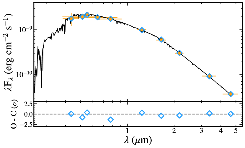
Figure 3: SED of TOI-1670. Broadband photometry (Section 3.1.2) is shown in orange circles, with horizontal errors representing the bandpass width. The best-fitting model SED is shown in black and blue diamonds are the model flux integrated over each bandpass. The residuals normalized by the photometric errors are shown in the bottom panel.

We estimate the mass of TOI-1670 using the stellar isochrone software package isochrones (Morton 2015a) and the MESA Isochrones and Stellar Tracks (MIST; Dotter 2016; Choi et al. 2016) evolutionary model grids. isochrones infers fundamental stellar parameters by comparing a variety of observational inputs to interpolated model values. We input the Gaia DR2 parallax, broadband photometry (2MASS $JHK_{s}$; Gaia DR2 $G$, $G_{\mathrm{BP}}$, and $B_{\mathrm{RP}}$; Johnson $V$ and $B$; and WISE $W1$ and $W2$), and the SME spectroscopic values ($T_{\mathrm{eff}}$, log$g$, and [Fe/H]) as priors. The posteriors are sampled using the MultiNest (Feroz et al. 2009, 2019) sampling algorithm.

All values for the stellar radius and mass are reported in Table 2. We include values from the TIC and Gaia DR2, as well as the typical mass and radius for an F7V dwarf for reference (Cox 2000). The SpecMatch-Emp fit also derives a stellar radius, which we couple to the calibration equations from Torres et al. (2010) to infer a surface gravity of log$g=4.14\pm 0.07$ dex and a stellar mass of $1.25\pm 0.09$ $M_{\odot}$. All values are in good agreement with each other. We adopt the ARIADNE radius ($R_{*}=1.316\pm 0.019$ $R_{\odot}$) and the isochrones mass ($M_{*}=1.21\pm 0.02$ $M_{\odot}$) as the stellar parameters to be used in the global fit, and report all adopted physical, photometric, and kinematic properties of TOI-1670 in Section 3.1.2.

Table 2: Stellar mass and radius of TOI-1670 derived from different methods.

Method	$M_{*}(M_{\odot})$	$R_{*}(R_{\odot})$
ARIADNE	$1.16\pm 0.16$	$1.316\pm 0.019$
isochrones	$1.21\pm 0.02$	$1.316\pm 0.007$
SpecMatch-Emp+Torres	$1.25\pm 0.09$	$1.57\pm 0.18$
TIC	$1.25\pm 0.18$	$1.312\pm 0.057$
Gaia DR2	$\cdots$	$1.38_{-0.07}^{+0.08}$
Typical F7V dwarf	1.21	1.32
Adopted	$1.21\pm 0.02$	$1.316\pm 0.019$

Note. — ^(a)Mass calculated using derived radius and log$g$. ^(b)Mass calculated using SpecMatch-Emp parameters and calibration equations from Torres et al. (2010). ^(c)Stassun et al. (2019). ^(d)Gaia Collaboration et al. (2018). ^(e)Cox (2000).

Table 3: Adopted Physical, Photometric, and Kinematic Properties of TOI-1670.

Parameter	Value	Source
TIC ID	441739020	1
TOI ID	1670	1
Gaia ID	1651911084230149248	2
2MASS ID	J17160415+7209402	3
Gaia $\alpha$ (J2000.0)	17:16:04.16	2
Gaia $\delta$ (J2000.0)	+72:09:40.17	2
Gaia Epoch	2015.5	2
Gaia Parallax (mas)	$5.92\pm 0.02$	2
Distance (pc)	$165.72_{-0.38}^{+0.32}$	4
Gaia $\mu_{\alpha}$cos$\delta$ (mas yr-1)	$-6.09\pm 0.05$	2
Gaia $\mu_{\delta}$ (mas yr-1)	$5.154\pm 0.05$	2
$B$ (mag)	$10.43\pm 0.03$	5
$V$ (mag)	$9.89\pm 0.03$	5
$T$ (mag)	$9.423\pm 0.0061$	1
$G$ (mag)	$9.8232\pm 0.0004$	2
$G_{RP}$ (mag)	$9.4145\pm 0.0014$	2
$G_{BP}$ (mag)	$10.0747\pm 0.0010$	2
$J$ (mag)	$8.97\pm 0.02$	3
$H$ (mag)	$8.75\pm 0.03$	3
$K_{s}$ (mag)	$8.724\pm 0.02$	3
$W1$ (mag)	$8.689\pm 0.023$	6
$W2$ (mag)	$8.702\pm 0.020$	6
$T_{\mathrm{eff}}$ (K)	$6170\pm 61$	This work
log $g$ (g cm-3)	$4.29\pm 0.11$	This work
[Fe/H] (dex)	$0.09\pm 0.07$	This work
$v$sin$i$ (km s-1)	$9.2\pm 0.6$	This work
$M_{*}$ ($M_{\odot}$)	$1.21\pm 0.02$	This work
$R_{*}$ ($R_{\odot}$)	$1.316\pm 0.019$	This work
$\rho_{*}$ (g cm-3)	$0.752\pm 0.036$	This work
Age (Gyr)	$2.53\pm 0.43$	This work
$A_{V}$ (mag)	$0.010\pm 0.006$	This work

References. — (1) Stassun et al. (2019), (2) Gaia Collaboration et al. (2018), (3) Cutri et al. (2003), (4) Bailer-Jones et al. (2021), (5) Høg et al. (2000), (6) Cutri et al. (2021)

3.2 Stellar Activity

Stellar activity in the form of rotationally modulated starspots and granulation can both mimic and mask the signals of planets in light curves (Llama & Shkolnik 2015, 2016) and radial velocities (e.g., Figueira et al. 2013). Thus, prior to running the global model fit, we first examine if stellar activity significantly influences the light curve and RV time series of TOI-1670. We measured a low average value of log$R^{\prime}_{\mathrm{HK}}=-4.93\pm 0.01$ from the HARPS-N spectra, which suggests that TOI-1670 is a quiet star not dominated by stellar activity (Mamajek & Hillenbrand 2008). The TESS light curve prior to detrending also does not exhibit any significant rotation or activity-induced variability.

A common statistical tool used to detect periodic signals in unevenly sampled time series data is the Lomb-Scargle periodogram (Lomb 1976; Scargle 1982). We utilize this algorithm to search for periodicity in both the TESS photometry and RV activity indicators to distinguish stellar activity-based signals from those induced by planetary motion. We compute the Generalized Lomb-Scargle periodograms (GLS; Zechmeister & Kürster 2009) for the “undetrended” PDCSAP light curve with the transit events removed, the RVs, the aforementioned activity indicators, and the spectral window function over the frequency range $0.0005-0.5$ d^-1 ($2-2000$ days) in Figure 4. The GLS power thresholds corresponding to false alarm probability (FAP) levels of 1% and 0.1% computed via a bootstrap approach are shown as dotted blue lines (Kuerster et al. 1997). The GLS periodogram for the RVs was computed for the combined HARPS-N and Tull coudé data, after subtracting the systematic velocity offsets as reported in Table 4. The periodogram of the TESS photometry has very low power with no peaks that have significance higher than the 1% FAP level. This is consistent with the flat nature of the undetrended PDCSAP light curve and indicates that TOI-1670 does not have a large starspot coverage fraction. The strongest signal in the periodogram of the RVs is at the $\sim$40.7 day orbital period of TOI-1670 c, which has a FAP $<$ 0.1%. This peak has no counterparts in the periodograms of the activity indices, which would be the case if that signal originated from stellar activity. Activity signals can also appear at the frequency of the stellar rotation period. Using the stellar radius and $v$sin$i$, we can place a lower limit of $P_{\mathrm{rot}}\geq 7.2$ d ($f\leq 0.138$ d^-1). No significant peaks are visible in the GLS periodogram of the $S$-indices at this frequency.

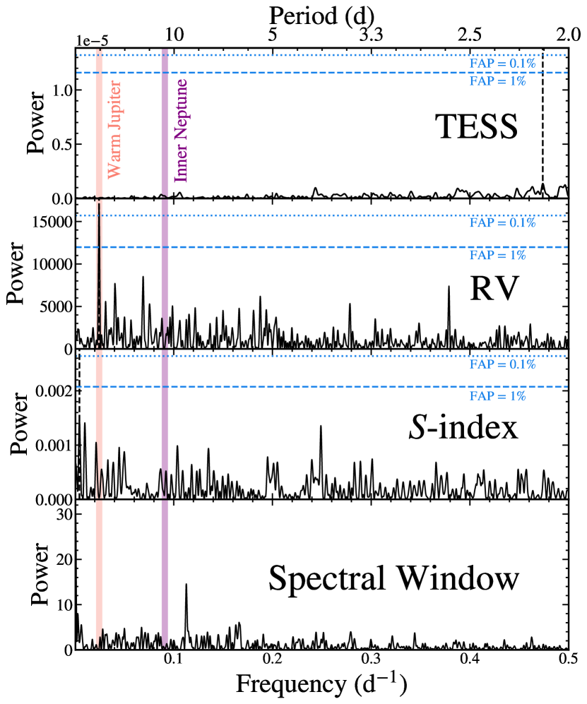
Figure 4: Lomb-Scargle periodograms of the undetrended TESS photometry after removing transit signals (top), combined Tull coudé and HARPS-N RVs after subtracting the systemic velocities (second), combined Mt. Wilson S-index from Tull coudé and HARPS-N spectra (third), and spectral window function (bottom). 1% and 0.1% FAP (blue dashed and dotted, respectively) lines are calculated using bootstrap resampling. The purple and pink vertical lines are the $\sim$10.9 and $\sim$40.7 d planetary signals determined by the TESS SPOC, respectively. The highest peak of each periodogram is shown as a dashed black vertical line. There are no counterpart peaks in the periodogram of the S-index that correspond to the $\sim$40.7 day signal seen in the periodogram of the RV, and no peaks rise above the 1% FAP threshold. No peaks are visible in the spectral window function periodogram. The only significant period ($<$0.1% FAP) in the RVs is at 41.1 d, consistent with the WJ (TOI-1670 c).

3.3 Statistical Validation of TOI-1670 b

Although TOI-1670 b is not significantly detected in the RV dataset, our model is able to place an upper limit on its mass. The $3\sigma$ upper limit of the fitted RV semi-amplitude is 14.5 m s^-1, which corresponds to an upper limit of 0.18 $M_{\mathrm{Jup}}$ for TOI-1670 b assuming an eccentricity of 0.

An estimate of the RV precision required to robustly detect TOI-1670 b can be made from a predicted mass inferred from its radius. Inputting the stellar and planetary parameters measured in Section 3 into a probabilistic mass-radius relation using the open software package forecaster (Chen & Kipping 2017) yields a mass estimate of $5.2_{-2.0}^{+4.0}$ $M_{\earth}$ for TOI-1670 b. Assuming a circular orbit, this corresponds to an RV semi-amplitude of $\sim$1.3 m s^-1. Robustly detecting an RV signal at this level requires an instrument precision at the 1 m s^-1 level and a well-behaved star.

We can exclude false positive scenarios to support TOI-1670 b as a likely planet using follow-up observations. From Gaia EDR3, we note that TOI-1670 has zero excess astrometric noise and a re-normalised unit weight error (RUWE) of 1.07, indicating that the single-star model is a good fit to the astrometric solution (Gaia Collaboration et al. 2018; Lindegren et al. 2018). From our radial velocities, we find that the overall RV variability is $<$110 m s^-1 from OES, $<$54 m s^-1 from TRES, $<$34 m s^-1 from the Tull coudé, and $<$16 m s^-1 from HARPS-N, all of which robustly exclude an eclipsing binary scenario for the host star.

Finally, we use TRICERATOPS (Giacalone et al. 2021) to statistically evaluate the probability of possible false positive scenarios involving nearby contaminant stars, including background eclipsing binaries. TRICERATOPS is a Bayesian tool for validating transiting planet candidates by modeling and calculating the probability of different scenarios that produce transit-like light curves. Based on the lack of a close stellar companion from Gaia astrometry, our high-resolution imaging, and our RVs, we omit the optional false positive calculations for the eclipsing binary and unresolved stellar companion scenarios in the TRICERATOPS code. TRICERATOPS returns a false positive probability (the total probability of a false positive scenario involving the primary star) of $<$0.015 and a nearby false positive probability (the sum of all false positive probabilities for scenarios involving nearby stars) of $<$10^-2. The RV confirmation of the outer coplanar transiting WJ further supports the planetary nature of TOI-1670 b as multi-planet systems are unlikely to be false positives (Lissauer et al. 2012; Rowe et al. 2014).

3.4 Joint Modeling of RVs & Photometry

We perform a multi-planet global fit to the available RV and transit observations of TOI-1670 using the pyaneti modeling suite (Barragán et al. 2019). As the planetary Doppler signals are not recovered at a significant level in the TRES and Ondřejov spectra, we only use the 49 Tull coudé and the 8 HARPS-N radial velocities in the modeling. We limit the light curve data to photometry spanning four full transit duration before and after all transit events of TOI-1670 b and c to improve computation efficiency; this results in a total of 24772 photometric points. These regions are colored purple and pink in Figure 1 for TOI 1670 b and c, respectively.

We simultaneously fit the Keplerian orbit and TESS light curve for 8 parameters: orbital period ($P$), central time of transit ($T_{0}$), RV semi-amplitude ($K$), transit impact parameter ($b$), planetary-to-stellar radius ($R_{\mathrm{p}}/R_{*}$), scaled semi-major axis ($a/R_{*}$), and parameterized forms of eccentricity and argument of periastron ($\sqrt{e}\>\mathrm{sin}\>\omega$ and $\sqrt{e}\>\mathrm{cos}\>\omega$). This last parametrization by Anderson et al. (2011) is used because the eccentricity posterior distribution for orbits with low $e$ and broad $\omega$ is poorly sampled by Markov chains (e.g., Lucy & Sweeney 1971; Ford 2006; Wang & Ford 2011). By defining $e$ and $\omega$ in a polar form, we avoid truncating the posterior distribution at zero and impose a uniform prior on $e$. We also adopt the parametrization of $b$ as defined by Winn (2010),

$$b=\frac{a\>\mathrm{cos}i_{*}}{R_{*}}\left(\frac{1-e^{2}}{1+e\mathrm{sin}\omega_{*}}\right),$$ (1)

where $i_{*}$ is the stellar inclination, in order to impose priors that exclude non-transiting orbits $(b>1+\frac{R_{p}}{R_{*}})$.

We set narrow uniform priors on both orbital period and time of transit based on visual inspection of the light curve and the SPOC preliminary parameters. For the inner sub-Neptune the ranges are $T_{0,b}=\mathcal{U}(1721.92,1721.99)$ in units of (BJD_TDB – 2457000) d, $P_{b}=\mathcal{U}(10.980,10.988)$ d, and $K_{b}=\mathcal{U}(0.0,10.0)$ m s^-1. For the outer Jupiter the ranges are $T_{0,c}=\mathcal{U}(1750.82,1750.92)$ in units of (BJD_TDB – 2457000) d, $P_{c}=\mathcal{U}(40.7485,40.7505)$ d, and $K_{c}=\mathcal{U}(10.0,100.0)$ m s^-1. The stellar mass and radius are also free parameters with Gaussian priors of $M_{*}=\mathcal{N}(1.215,0.023)\;M_{\odot}$ and $R_{*}=\mathcal{N}(1.316,0.019)\;R_{\odot}$. These parameters are further constrained by the stellar mean density, which is affected by $P$ and $a/R_{*}$ (Seager & Mallén-Ornelas 2003; Winn 2010). We assumed a quadratic limb-darkening law following the equations from Mandel & Agol (2002), who define the linear and quadratic coefficients as $u_{1}$ and $u_{2}$, respectively. The parameterization of $q_{1}=(u_{1}+u_{2})^{2}$ and $q_{2}=0.5u_{1}(u_{1}+u_{2})^{-1}$ from Kipping (2013) is adopted. We set broad uniform priors for all other parameters and report them in Table 4. A “jitter” term is added to the radial velocities to account for any systematic and astrophysical variance not reported in the observational uncertainties.

Posterior distributions of fitted and derived parameters were sampled using an MCMC Metropolis-Hasting algorithm following the description by Sharma (2017) as implemented by pyaneti. The distributions were sampled using 50 chains for 10000 iterations with a thinning factor of 10. The convergence of each chain was determined with the Gelman-Rubin diagnostic test (Gelman & Rubin 1992).

Using the TESS photometry and RVs, we jointly model the transits of TOI-1670 b and c and the RV curve of TOI-1670 c using the priors as previously described. The posterior values of the fitted and derived system parameters from pyaneti for TOI-1670 are given in Table 4. The best-fitting phased TESS light curves for TOI-1670 b and c and RV model for TOI-1670 c are plotted in Figures 5–7. Figure 9 in Appendix C displays the posterior distributions for fitted parameters. We find a mass, radius, and density of TOI-1670 c of $M_{\mathrm{c}}=0.63_{-0.08}^{+0.09}$ $M_{\mathrm{Jup}}$, $R_{\mathrm{c}}=0.987_{-0.025}^{+0.025}$ $R_{\mathrm{Jup}}$, and $\rho_{\mathrm{c}}=0.81_{-0.11}^{+0.13}$ g cm^-3, respectively. For TOI-1670 b, we find a radius of $2.06_{-0.15}^{+0.19}$ $R_{\earth}$ and a $3\sigma$ mass upper limit of $M_{\mathrm{b}}<0.13$ $M_{\mathrm{Jup}}$.

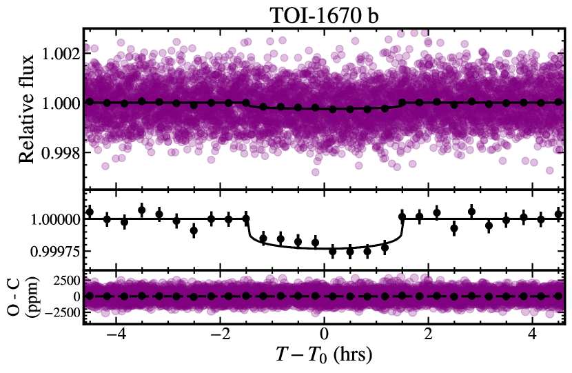
Figure 5: Transit light curve folded to the orbital period of TOI-1670 b. The TESS photometry are shown in purple and the solid black line is the best-fitting transit model. The black circles are the photometric data binned over 20-minute intervals. The middle panel zooms in on the best-fit transit model and binned data points. The fit residuals are shown in the lower panel.

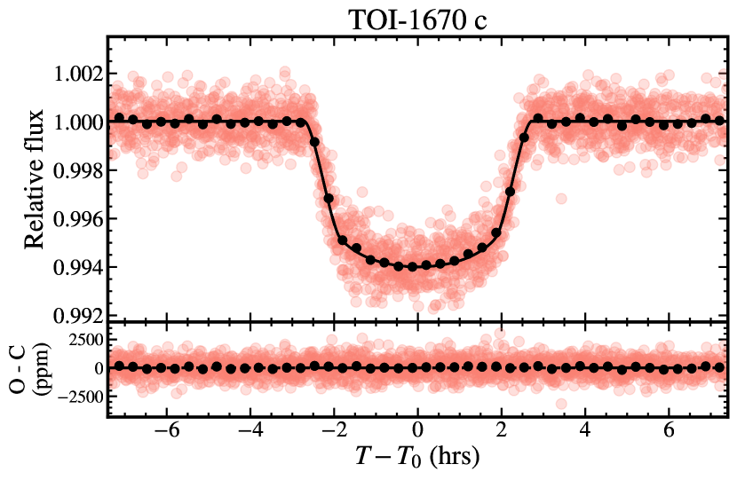
Figure 6: Transit light curve folded to the orbital period of TOI-1670 c. The TESS photometry are shown in pink and the solid black line is the best-fitting transit model. Black points are the photometric data binned over 20-minute intervals.

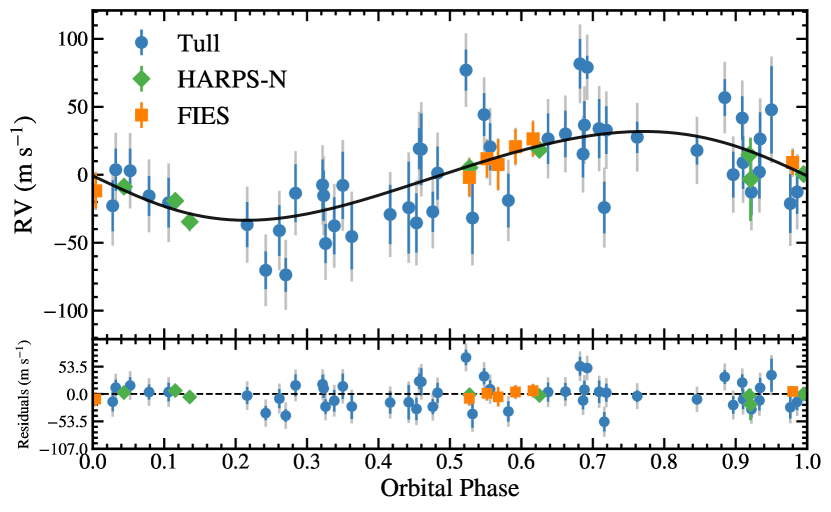
Figure 7: RV curve of TOI-1670 phase folded to the orbital period of the WJ, TOI-1670 c, with the contributions of the inner companion removed. The different color points denote the different spectrographs, and the best-fitting RV model is shown in the solid black line. The fit residuals are shown in the lower panel. The colored error bars are nominal RV errors and the grey error bars include the systematic jitter term.

Table 4: Priors and Posteriors on Global System Parameters of TOI-1670 b and c.

	Adopted Prior		Posterior Values
Fitted Parameters	$b$	$c$	$b$	$c$
$T_{0}$ (BJDTDB$-2457000$)	$\mathcal{U}(1721.92,1721.99)$	$\mathcal{U}(1750.82,1750.92)$	$1721.9423_{-0.0062}^{+0.0071}$	$1750.88286_{-0.00083}^{+0.00085}$
$P$ (days)	$\mathcal{U}(10.980,10.988)$	$\mathcal{U}(40.7485,40.7505)$	$10.98462_{-0.00051}^{+0.00046}$	$40.74976_{-0.00021}^{+0.000022}$
$K$ (m s-1)	$\mathcal{U}(0.0,10.0)$	$\mathcal{U}(10.0,100)$	$4.6_{-3.0}^{+3.3}$	$32.7_{-4.3}^{+4.7}$
$b$	$\mathcal{U}(0.0,1.0)$	$\mathcal{U}(0.0,1.0)$	$0.61_{-0.37}^{+0.22}$	$0.76_{-0.04}^{+0.02}$
$a/R_{*}$	$\mathcal{U}(1.1,20.0)$	$\mathcal{U}(1.1,50.0)$	$16.88_{-0.27}^{+0.27}$	$40.68_{-0.66}^{+0.66}$
$R_{\mathrm{p}}/R_{*}$	$\mathcal{U}(0.0,0.05)$	$\mathcal{U}(0.0,0.15)$	$0.014_{-0.001}^{+0.001}$	$0.077_{-0.002}^{+0.002}$
$\sqrt{e}$ sin $\omega$	$\mathcal{U}(-1.0,1.0)$	$\mathcal{U}(-1.0,1.0)$	$0.18_{-0.44}^{+0.36}$	$0.27_{-0.10}^{+0.08}$
$\sqrt{e}$ cos $\omega$	$\mathcal{U}(-1.0,1.0)$	$\mathcal{U}(-1.0,1.0)$	$-0.63_{-0.21}^{+0.62}$	$-0.07_{-0.13}^{+0.14}$
Derived Parameters
$M_{p}$	$\cdots$	$\cdots$	$13.8_{-8.7}^{+9.5}$ $M_{\earth}$	$0.63_{-0.08}^{+0.09}$ $M_{\mathrm{Jup}}$
$R_{p}$	$\cdots$	$\cdots$	$2.06_{-0.15}^{+0.19}$ $R_{\earth}$	$0.987_{-0.025}^{+0.025}$ $R_{\mathrm{Jup}}$
$\rho_{p}$ (g cm-3)	$\cdots$	$\cdots$	$8.6_{-5.6}^{+6.9}$	$0.81_{-0.11}^{+0.13}$
$e$	$\cdots$	$\cdots$	$0.59_{-0.26}^{+0.17}$	$0.09_{-0.04}^{+0.05}$
$\omega$ (deg)	$\cdots$	$\cdots$	$163.6_{-53.7}^{+41.7}$	$105.5_{-29.4}^{+28.6}$
$i$ (deg)	$\cdots$	$\cdots$	$86.87_{-1.07}^{+1.16}$	$88.84_{-0.04}^{+0.04}$
$a$ (AU)	$\cdots$	$\cdots$	$0.103_{-0.002}^{+0.002}$	$0.249_{-0.005}^{+0.005}$
$T_{14}$ (hrs)	$\cdots$	$\cdots$	$2.80_{-0.19}^{+0.16}$	$5.40_{-0.05}^{+0.06}$
$T_{eq}$ (K)	$\cdots$	$\cdots$	$1062_{-13}^{+14}$	$684_{-9}^{+9}$
Additional Parameters
$M_{*}$ (from scaled parameters) ($M_{\odot}$)	$\mathcal{N}(1.215,0.023)$		$1.218_{-0.076}^{+0.081}$	$1.239_{-0.079}^{+0.084}$
$\rho_{*}$ (from transit) (g cm-3)	$\cdots$		$0.754_{-0.035}^{+0.037}$	$0.767_{-0.037}^{+0.038}$
$q_{1}$	$\mathcal{U}(0.0,1.0)$		$0.35_{-0.11}^{+0.19}$
$q_{2}$	$\mathcal{U}(0.0,1.0)$		$0.32_{-0.23}^{+0.39}$
$\gamma_{\mathrm{Tull}}$ (km s-1)	$\mathcal{U}(-3.6849,-3.3299)$		$-3.5132_{-0.0043}^{+0.0042}$
$\gamma_{\mathrm{FIES}}$ (km s-1)	$\mathcal{U}(-0.1217,0.1139)$		$-0.0108_{-0.0061}^{+0.0061}$
$\gamma_{\mathrm{HARPS-N}}$ (km s-1)	$\mathcal{U}(-11.6134,-11.3602)$		$-11.4805_{-0.0027}^{+0.0025}$
RV jitter (Tull) (m s-1)	$\cdots$		$22.5_{-3.6}^{+3.9}$
RV jitter (FIES) (m s-1)	$\cdots$		$5.3_{-3.8}^{+7.2}$
RV jitter (HARPS-N) (m s-1)	$\cdots$		$4.3_{-2.8}^{+4.5}$

4 Discussion

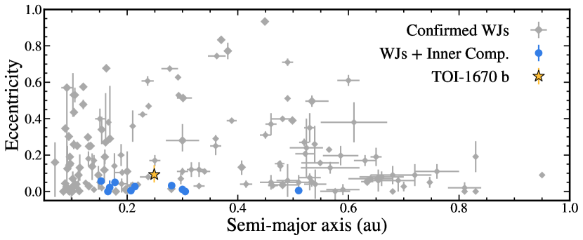
Figure 8: Eccentricity as a function of semi-major axis for confirmed WJ systems. Multi-planet systems with an outer WJ and a smaller, inner companion are shown in blue circles whereas all other WJs are plotted in grey diamonds. TOI-1670 is denoted with the yellow star. Systems with a similar configuration as TOI-1670 all have low eccentricities, suggesting a gentle formation pathway. Planet orbital parameters are assembled from exoplanet.eu (Schneider et al. 2011) and the NASA Exoplanet Archive (Akeson et al. 2013; NASA Exoplanet Archive 2021) as of June 2021.

Table 5: Confirmed systems with an outer warm giant planet and at least one smaller inner companion.

System	$M_{\mathrm{in}}$	$R_{\mathrm{in}}$	$P_{\mathrm{in}}$	$M_{\mathrm{out}}$	$R_{\mathrm{out}}$	$P_{\mathrm{out}}$	$e_{\mathrm{out}}$	$\sigma_{e}$	$P_{\mathrm{out}}$/$P_{\mathrm{in}}$	Ref.
	$(M_{\mathrm{Jup}})$	$(R_{\mathrm{Jup}})$	(d)	$(M_{\mathrm{Jup}})$	$(R_{\mathrm{Jup}})$	(d)
Kepler-89	$<$0.05	0.385	10.42	0.33	1.005	22.34	0.022	$0.038$	2.14	1, 2
TOI-216	0.06	0.714	17.16	0.56	0.901	34.53	0.0046	${}^{+0.0027}_{-0.0012}$	2.01	3, 4
Kepler-117	0.09	0.719	18.80	1.84	1.101	50.79	0.0323	$0.0033$	2.70	5, 6
Kepler-30	0.03	0.348	29.22	1.69	1.097	60.32	0.011	$0.001$	2.06	7, 8
HIP 57274	0.04	$\cdots$	8.14	0.41	$\cdots$	32.03	0.05	$0.03$	3.94	9
GJ 876	0.76	$\cdots$	30.13	2.39	$\cdots$	61.08	0.027	$0.002$	2.03	10
K2-290	$<$0.07	0.273	9.21	0.77	1.006	48.37	0 (fixed)	$<$0.241	5.25	11
Kepler-56	0.07	0.581	10.50	0.57	0.874	21.40	0.00	$0.01$	2.04	12, 13
Kepler-88	0.03	0.307	10.92	0.67	$\cdots$	22.26	0.0572	$0.0005$	2.04	14
Kepler-289	0.01	0.239	66.06	0.42	1.034	125.85	0.005	$0.015$	1.91	15
TOI-1670	$<$0.13	0.184	10.98	0.63	0.987	40.75	0.09	${}_{-0.04}^{+0.05}$	3.71	This work

Note. — ^(a)1$\sigma$ uncertainties or 3$\sigma$ upper limit on $e_{\mathrm{out}}$. ^(b)Minimum mass, $M_{p}$sin$i$. ^(c)Mass determined assuming coplanar model with fixed inclinations.

References. — (1) Hirano et al. (2012), (2) Weiss et al. (2013), (3) Dawson et al. (2019), (4) Dawson et al. (2021), (5) Rowe et al. (2014), (6) Bruno et al. (2015), (7) Sanchis-Ojeda et al. (2012), (8) Panichi et al. (2018), (9) Fischer et al. (2012), (10) Trifonov et al. (2018), (11) Hjorth et al. (2019), (12) Huber et al. (2013), (13) Otor et al. (2016), (14) Weiss et al. (2020), (15) Schmitt et al. (2014).

The existence of WJ systems hosting one or more smaller coplanar inner companions such as TOI-1670 is inconsistent with dynamical migration routes. During high-eccentricity tidal migration, multiple close-in planets would likely interact with each other and potentially lead to ejections or collisions (e.g., Rasio & Ford 1996; Chatterjee et al. 2008; Mustill et al. 2015). Similarly, planet-planet scattering and Von Zeipel–Lidov–Kozai interactions require an outer companion (Veras & Armitage 2005; Anderson & Lai 2017). Multi-planet systems hosting a WJ with low eccentricity represent another type of system that experienced comparatively gentle dynamical histories such as inward disk migration or in situ formation.

TOI-1670 joins a handful of confirmed systems with an outer warm, giant exoplanet ($M_{p}>0.25$ $M_{\mathrm{Jup}}$, $10<P<200$ d) and at least one inner, smaller companion (see Section 4). Figure 8 shows the eccentricity versus semi-major axis of confirmed WJs. WJs in all 11 systems (including TOI-1670) with similar configurations have low eccentricities, whereas the eccentricities of other WJs without known inner companions are widely distributed. This divergence further suggests that this group of TOI-1670-like systems may have formed and migrated along a similar evolutionary pathway.

One way to disentangle whether disk migration or in situ formation plays the dominant role in sculpting these multi-planet systems is by examining their period ratios in search of near mean-motion resonances (MMRs). Disk migration is expected to efficiently capture giant planets into MMRs close to small integer period ratios such as 2:1, 3:1, 3:2, and 4:3 (e.g., Goldreich & Tremaine 1980; Lee & Peale 2001; Armitage 2010; Winn & Fabrycky 2015). In situ formation can also create planets in orbital resonances, either coincidentally or by eccentricity damping via interactions with the protoplanetary or planetesimal disk (Dawson et al. 2016; Morrison et al. 2020). In this formation scenario there should be a population of systems that congregate at or near these different integer ratios.

Within the sample of 11 known systems that have a giant planet with a small inner companion, 8 WJs (73%) are in or near a 2:1 or 3:1 resonance with the inner planet (Section 4). With a period ratio of 3.7, TOI-1670 joins two other systems, K2-290 and HIP 57274, that have non-MMR orbital period ratios greater than 3. The planets in these systems may have formed in situ or migrated inward together. Alternatively, that the planets in these systems are not locked in an MMR could also indicate that they formed independently and did not migrate together or became unstable over time (Pichierri & Morbidelli 2020; Petit et al. 2020; Izidoro et al. 2021). This may hint at a division within this small class of WJs in multi-planet systems in which some migrate into place via disk migration (those with integer period ratios) while others formed where we see them today or experienced further dynamical interaction later in their lifetime. This hypothesis can be further investigated by increasing the number of warm giant planets with smaller inner companions and examining population trends within this sample.

Appendix A RV measurements

Table 6 records the reconnaissance RV measurements for TOI-1670. Table 7 lists the relative Tull coudé and HARPS-N precise RVs used in the joint global orbit fit of TOI-1670. See Section 2 for details.

Table 6: Reconnaissance RV Measurements

BJDTDB	RV (m s-1)	$\sigma_{\mathrm{RV}}$ (m s-1)	Instrument
2458882.039318	0.0	53.0	TRES
2458900.020153	47.3	51.0	TRES
2458915.012011	24.0	55.2	TRES
2458917.976858	154.6	50.7	TRES
2458925.016694	120.9	59.5	TRES
2459037.890277	47.8	53.0	TRES
2458891.503545280	$-44487.8$	65.5	OES
2458894.510498418	$-44361.4$	235.5	OES
2458930.563753183	$-44463.7$	148.9	OES
2458931.473755364	$-44129.3$	133.1	OES
2458931.513916946	$-44314.2$	86.1	OES
2458936.492023797	$-44303.4$	78.8	OES
2458937.487545487	$-44271.6$	96.2	OES
2458945.510337937	$-44305.1$	79.2	OES
2458947.486183500	$-44194.3$	142.3	OES
2458953.506692706	$-44245.2$	144.2	OES
2458956.498833757	$-44480.6$	101.3	OES
2458956.517247843	$-44259.6$	89.7	OES
2458957.559932472	$-44282.0$	127.1	OES
2458959.481333630	$-44108.1$	164.9	OES
2458959.523497538	$-44053.2$	90.4	OES
2458959.503590371	$-44141.2$	68.8	OES
2458960.545742497	$-44363.6$	77.3	OES
2458961.436750593	$-44160.5$	143.6	OES
2458963.472548647	$-44261.4$	85.7	OES
2458962.515129209	$-44262.5$	59.6	OES
2458964.553762859	$-44301.1$	84.5	OES
2458967.598704441	$-44164.8$	61.7	OES
2458976.525095871	$-44269.5$	102.3	OES
2458989.502480241	$-44023.8$	108.6	OES
2458991.474925697	$-44320.5$	124.4	OES
2459002.550308453	$-44299.1$	114.2	OES
2459067.550946345	$-44228.8$	162.3	OES
2459071.496445452	$-44133.1$	125.1	OES
2459074.552383421	$-44246.4$	119.8	OES
2459100.533604675	$-44300.5$	145.7	OES
2459101.536958157	$-44393.2$	96.2	OES
2459104.526104830	$-44470.6$	65.0	OES

Table 7: Relative RV Measurements Used in Orbit Fit

BJDTDB	RV	$\sigma_{\mathrm{RV}}$	Instrument	S-index	$\sigma_{\mathrm{S-index}}$	BIS	FWHM
(d)	(m s-1)	(m s -1)				(m s-1)	(km s-1)
2459073.581564	$-11469.3$	3.7	HARPS-N	$0.158$	$0.001$	24.3	13.764
2459082.412035	$-11513.4$	5.6	HARPS-N	$0.161$	$0.002$	31.2	13.816
2459098.371706	$-11475.3$	3.1	HARPS-N	$0.160$	$0.001$	16.8	13.780
2459102.360849	$-11460.2$	3.6	HARPS-N	$0.159$	$0.001$	16.0	13.733
2459114.404597	$-11481.9$	30.5	HARPS-N	$\cdots$	$\cdots$	74.8	13.744
2459117.430022	$-11482.9$	4.1	HARPS-N	$0.164$	$0.002$	27.0	13.806
2459119.408423	$-11490.8$	3.5	HARPS-N	$0.158$	$0.001$	26.2	13.743
2459122.336070	$-11498.2$	2.9	HARPS-N	$0.160$	$0.001$	6.9	13.758
2458994.555398	$0.0$	$9.2$	FIES	$\cdots$	$\cdots$	10.2	18.393
2458995.551629	$-21.7$	$13.0$	FIES	$\cdots$	$\cdots$	41.2	18.509
2459018.504159	$-5.7$	$18.6$	FIES	$\cdots$	$\cdots$	32.4	18.365
2459019.496162	$3.7$	$12.8$	FIES	$\cdots$	$\cdots$	22.7	18.411
2459020.497833	$13.9$	$12.7$	FIES	$\cdots$	$\cdots$	7.4	18.458
2459098.364441	$-12.7$	$13.8$	FIES	$\cdots$	$\cdots$	16.8	18.394
2459099.369294	$1.9$	$13.6$	FIES	$\cdots$	$\cdots$	24.0	18.442
2458950.979568	$-3502.7$	$19.3$	Tull coudé	$0.20$	$0.03$	$\cdots$	$\cdots$
2458951.909478	$-3510.9$	$19.5$	Tull coudé	$0.21$	$0.03$	$\cdots$	$\cdots$
2458957.843670	$-3527.2$	$14.6$	Tull coudé	$0.21$	$0.03$	$\cdots$	$\cdots$
2458958.958375	$-3531.9$	$18.2$	Tull coudé	$0.19$	$0.03$	$\cdots$	$\cdots$
2458982.835596	$-3432.2$	$08.5$	Tull coudé	$0.20$	$0.03$	$\cdots$	$\cdots$
2458983.927587	$-3478.8$	$17.5$	Tull coudé	$0.19$	$0.03$	$\cdots$	$\cdots$
2458994.813377	$-3524.2$	$16.1$	Tull coudé	$0.19$	$0.02$	$\cdots$	$\cdots$
2459047.698935	$-3524.8$	$21.3$	Tull coudé	$0.20$	$0.03$	$\cdots$	$\cdots$
2459054.754109	$-3493.7$	$15.1$	Tull coudé	$0.19$	$0.03$	$\cdots$	$\cdots$
2459054.873732	$-3494.0$	$26.4$	Tull coudé	$0.19$	$0.03$	$\cdots$	$\cdots$
2459055.802778	$-3510.8$	$19.5$	Tull coudé	$0.19$	$0.02$	$\cdots$	$\cdots$
2459072.664836	$-3512.6$	$16.9$	Tull coudé	$0.19$	$0.02$	$\cdots$	$\cdots$
2459073.701460	$-3530.7$	$16.8$	Tull coudé	$0.19$	$0.02$	$\cdots$	$\cdots$
2459090.659723	$-3548.9$	$21.0$	Tull coudé	$0.19$	$0.02$	$\cdots$	$\cdots$
2459091.655351	$-3556.7$	$24.2$	Tull coudé	$0.20$	$0.02$	$\cdots$	$\cdots$
2459104.674112	$-3429.9$	$18.2$	Tull coudé	$\cdots$	$\cdots$	$\cdots$	$\cdots$
2459115.597718	$-3463.8$	$32.1$	Tull coudé	$0.20$	$0.03$	$\cdots$	$\cdots$
2459116.673732	$-3534.0$	$21.7$	Tull coudé	$0.19$	$0.02$	$\cdots$	$\cdots$
2459134.594159	$-3540.6$	$21.8$	Tull coudé	$0.18$	$0.02$	$\cdots$	$\cdots$
2459135.654423	$-3535.4$	$33.8$	Tull coudé	$0.20$	$0.02$	$\cdots$	$\cdots$
2459143.603909	$-3485.6$	$18.6$	Tull coudé	$0.20$	$0.02$	$\cdots$	$\cdots$
2459144.595144	$-3481.6$	$17.1$	Tull coudé	$0.18$	$0.03$	$\cdots$	$\cdots$
2459145.600434	$-3496.1$	$17.2$	Tull coudé	$0.19$	$0.02$	$\cdots$	$\cdots$
2459171.552605	$-3528.1$	$18.6$	Tull coudé	$0.20$	$0.02$	$\cdots$	$\cdots$
2459228.014988	$-3486.3$	$21.8$	Tull coudé	$0.20$	$0.03$	$\cdots$	$\cdots$
2459241.016167	$-3536.2$	$18.8$	Tull coudé	$0.20$	$0.03$	$\cdots$	$\cdots$
2459242.012350	$-3509.5$	$16.2$	Tull coudé	$0.19$	$0.02$	$\cdots$	$\cdots$
2459242.012350	$-3509.5$	$16.2$	Tull coudé	$0.18$	$0.02$	$\cdots$	$\cdots$
2459270.939084	$-3486.9$	$11.5$	Tull coudé	$0.19$	$0.02$	$\cdots$	$\cdots$
2459275.930375	$-3455.1$	$13.6$	Tull coudé	$\cdots$	$\cdots$	$\cdots$	$\cdots$
2459276.929526	$-3469.8$	$16.0$	Tull coudé	$0.18$	$0.02$	$\cdots$	$\cdots$
2459277.949543	$-3484.9$	$19.6$	Tull coudé	$0.18$	$0.03$	$\cdots$	$\cdots$
2459281.939450	$-3510.8$	$15.5$	Tull coudé	$0.18$	$0.02$	$\cdots$	$\cdots$
2459293.909641	$-3570.9$	$14.4$	Tull coudé	$0.17$	$0.02$	$\cdots$	$\cdots$
2459294.893907	$-3523.4$	$24.7$	Tull coudé	$0.18$	$0.02$	$\cdots$	$\cdots$
2459301.921161	$-3434.4$	$15.1$	Tull coudé	$0.14$	$0.02$	$\cdots$	$\cdots$
2459302.952236	$-3467.8$	$15.7$	Tull coudé	$0.18$	$0.02$	$\cdots$	$\cdots$
2459309.807855	$-3535.6$	$19.0$	Tull coudé	$0.18$	$0.03$	$\cdots$	$\cdots$
2459339.846070	$-3548.9$	$21.8$	Tull coudé	$0.18$	$0.03$	$\cdots$	$\cdots$
2459340.775733	$-3539.7$	$14.8$	Tull coudé	$0.19$	$0.02$	$\cdots$	$\cdots$
2459355.848218	$-3493.3$	$10.4$	Tull coudé	$0.20$	$0.03$	$\cdots$	$\cdots$
2459372.775403	$-3554.6$	$18.7$	Tull coudé	$0.19$	$0.03$	$\cdots$	$\cdots$
2459383.791707	$-3545.3$	$26.6$	Tull coudé	$0.18$	$0.02$	$\cdots$	$\cdots$
2459384.793846	$-3491.9$	$17.4$	Tull coudé	$0.18$	$0.02$	$\cdots$	$\cdots$
2459385.835820	$-3530.8$	$19.8$	Tull coudé	$\cdots$	$\cdots$	$\cdots$	$\cdots$
2459411.687127	$-3548.1$	$16.6$	Tull coudé	$\cdots$	$\cdots$	$\cdots$	$\cdots$
2459412.744002	$-3582.4$	$13.9$	Tull coudé	$\cdots$	$\cdots$	$\cdots$	$\cdots$
2459454.638202	$-3584.9$	$12.5$	Tull coudé	$\cdots$	$\cdots$	$\cdots$	$\cdots$
2459456.737608	$-3519.6$	$18.8$	Tull coudé	$\cdots$	$\cdots$	$\cdots$	$\cdots$
2459471.673405	$-3476.9$	$17.6$	Tull coudé	$\cdots$	$\cdots$	$\cdots$	$\cdots$

Appendix B Model Complexity and Selection

Model selection balances the quality of the model fit and the model complexity, or number of parameters. Including extraneous parameters can lead to over-fitting of the data while excluding physically-motivated aspects of the model can result in under-fitting of the data and introduce bias. Our model fit is susceptible to the former scenario when we consider parameters that can not be robustly estimated from the data, such as the mass of the sub-Neptune or the eccentricities of either planet.

Here we assess whether two alternative less complex models are more justified by the data using different model selection criteria. We first compare model fits using only the RV data (excluding the light curve) for a one- and two-planet model, whereby we exclude the inner sub-Neptune in the one-planet fit. In the second comparison, we examine two joint model fits, one where the WJ eccentricity is fixed to zero and another in which the WJ eccentricity is a free parameter. In both cases, the inner sub-Neptune is not modeled with the RVs and its eccentricity is fixed to zero.

Several metrics can be used to establish whether a model is justified by the data. For each fit, pyaneti reports the Bayesian Information Criterion (BIC; Schwarz 1978; Raftery 1986), defined as

$$\text{BIC}\equiv-2\>\text{ln}\>\mathcal{L}+k\>\text{ln}\>N,$$ (B1)

and the Akaike Information Criterion (AIC; Akaike 1998), defined as

$$\text{AIC}\equiv-2\>\text{ln}\>\mathcal{L}+2k.$$ (B2)

Here, $\mathcal{L}$ is the model likelihood, $k$ is the number of model parameters, and $N$ is the number of data points used in the fit. We further calculate the AIC corrected for small sample sizes (AIC_c; Sugiura 1978; Burnham & Anderson 2004):

$$\text{AIC\textsubscript{c}}=\text{AIC}+\frac{2k(k+1)}{N-k-1}.$$ (B3)

This metric is preferred over the AIC as it can be understood as a relative model likelihood using Akaike weights (Akaike 1981; Burnham & Anderson 2004; Liddle 2007), where the weight $w$ for each model $i$ is

$$w_{i}=\frac{e^{-\Delta\text{AIC\textsubscript{c,$i$}}/2}}{\sum_{r=1}^{R}e^{-\Delta\text{AIC\textsubscript{c,$r$}}/2}}.$$ (B4)

These metrics take into account the model likelihood while penalizing each additional free parameter. The BIC can be interpreted as a model evidence ratio, such that according to the Jeffreys’ scale a BIC difference between two models of $\geq$5 is strong evidence and $\geq$10 is decisive evidence against the model with a higher BIC (Jeffreys 1935; Kass & Raftery 1995; Liddle 2007).

We find that both the BIC and Akaike weights criteria favor the one-planet model for the RV data and the WJ circular orbit model in the global joint fits. For the RV-only fits, we find $\mathrm{BIC}=-269.3$, $\mathrm{AIC}=-297.3$, $\mathrm{AIC}_{\mathrm{c}}=-290.1$, and an Akaike weight of $>$0.99 for the one-planet only model and $\mathrm{BIC}=-254.0$, $\mathrm{AIC}=-288.5$, $\mathrm{AIC}_{\mathrm{c}}=-277.0$, and an Akaike weight of $<$0.01 for the two-planet model. The BIC comparison ($\Delta\text{BIC}>15$) and the Akaike weight (99% relative likelihood) strongly favor the one-planet model fit. In the global joint fits, we find $\mathrm{BIC}=-283106.1$, $\mathrm{AIC}=-283260.4$, $\mathrm{AIC}_{\mathrm{c}}=-283260.3$, and an Akaike weight of 0.85 for the zero-eccentricity global model and $\mathrm{BIC}=-283086.4$, $\mathrm{AIC}=-283256.9$, $\mathrm{AIC}_{\mathrm{c}}=-283256.9$, and an Akaike weight of 0.15 for the free eccentricity global model. Both the BIC comparison ($\Delta\text{BIC}>15$) and the Akaike weights (85% relative likelihood) suggest that there is strong evidence in favor of the circular orbit model.

Despite these model selection preferences, we find that the final parameter uncertainties are slightly underestimated when compared to the full model fit, which suggests that the less complex models are under-fitting the data. Orbital parameter uncertainties are larger by approximately 10–50% in the full global model (which includes the smaller, inner planet and the eccentricities of both planets) compared to the more simple, fixed zero-eccentricity joint model. For example, the uncertainties of the orbital period, planet mass, and planet radius of the WJ increased by 10%, 30%, and 40%, respectively. By neglecting the smaller, inner planet and the eccentricity of either planet in order to avoid over-fitting the data, the simpler model artificially underestimates the uncertainties of other model parameters. Ultimately, to more accurately determine parameter uncertainties, we adopt the global simultaneous joint model fit and report upper limits on parameter posteriors when robust detections are not possible.

Appendix C Posterior distributions of fitted parameters

Figure 9 displays the posterior distributions of fitted parameters from the global joint fit. See Section 3.4 for more details.

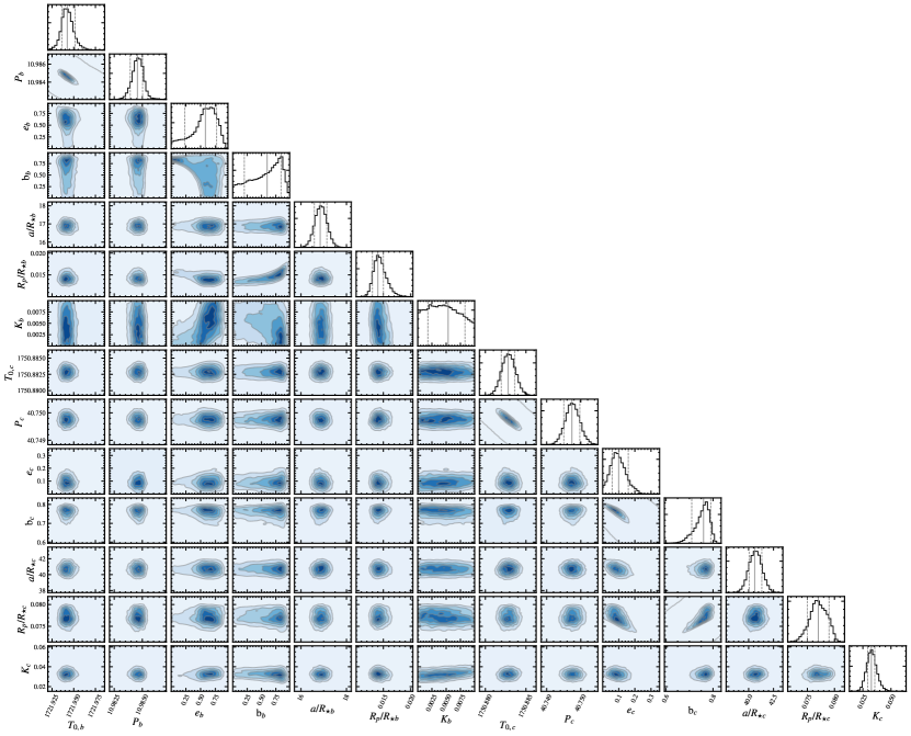
Figure 9: Posterior distributions of fitted parameters for TOI-1670 b and c derived from joint global fit of RVs and light curve.

References

- Akaike (1981) Akaike, H. 1981, Journal of Econometrics, 16, 3. https://EconPapers.repec.org/RePEc:eee:econom:v:16:y:1981:i:1:p:3-14
- Akaike (1998) —. 1998, Information Theory and an Extension of the Maximum Likelihood Principle, ed. E. Parzen, K. Tanabe, & G. Kitagawa (New York, NY: Springer New York), 199–213, doi: 10.1007/978-1-4612-1694-0_15
- Akeson et al. (2013) Akeson, R. L., Chen, X., Ciardi, D., et al. 2013, PASP, 125, 989, doi: 10.1086/672273
- Albrecht et al. (2012) Albrecht, S., Winn, J. N., Johnson, J. A., et al. 2012, ApJ, 757, 18, doi: 10.1088/0004-637X/757/1/18
- Allard et al. (2011) Allard, F., Homeier, D., & Freytag, B. 2011, in Astronomical Society of the Pacific Conference Series, Vol. 448, 16th Cambridge Workshop on Cool Stars, Stellar Systems, and the Sun, ed. C. Johns-Krull, M. K. Browning, & A. A. West, 91. https://arxiv.org/abs/1011.5405
- Anderson et al. (2011) Anderson, D. R., Collier Cameron, A., Hellier, C., et al. 2011, ApJ, 726, L19, doi: 10.1088/2041-8205/726/2/L19
- Anderson & Lai (2017) Anderson, K. R., & Lai, D. 2017, MNRAS, 472, 3692, doi: 10.1093/mnras/stx2250
- Anderson et al. (2020) Anderson, K. R., Lai, D., & Pu, B. 2020, MNRAS, 491, 1369, doi: 10.1093/mnras/stz3119
- Anderson et al. (2016) Anderson, K. R., Storch, N. I., & Lai, D. 2016, MNRAS, 456, 3671, doi: 10.1093/mnras/stv2906
- Armitage (2010) Armitage, P. J. 2010, Astrophysics of Planet Formation
- Astropy Collaboration et al. (2018) Astropy Collaboration, Price-Whelan, A. M., Sipőcz, B. M., et al. 2018, AJ, 156, 123, doi: 10.3847/1538-3881/aabc4f
- Bailer-Jones et al. (2021) Bailer-Jones, C. A. L., Rybizki, J., Fouesneau, M., Demleitner, M., & Andrae, R. 2021, AJ, 161, 147, doi: 10.3847/1538-3881/abd806
- Barragán et al. (2019) Barragán, O., Gandolfi, D., & Antoniciello, G. 2019, MNRAS, 482, 1017, doi: 10.1093/mnras/sty2472
- Batygin (2012) Batygin, K. 2012, Nature, 491, 418, doi: 10.1038/nature11560
- Batygin et al. (2016) Batygin, K., Bodenheimer, P. H., & Laughlin, G. P. 2016, ApJ, 829, 114, doi: 10.3847/0004-637X/829/2/114
- Boley et al. (2016) Boley, A. C., Granados Contreras, A. P., & Gladman, B. 2016, ApJ, 817, L17, doi: 10.3847/2041-8205/817/2/L17
- Bruno et al. (2015) Bruno, G., Almenara, J. M., Barros, S. C. C., et al. 2015, A&A, 573, A124, doi: 10.1051/0004-6361/201424591
- Bruntt et al. (2010) Bruntt, H., Bedding, T. R., Quirion, P. O., et al. 2010, MNRAS, 405, 1907, doi: 10.1111/j.1365-2966.2010.16575.x
- Buchhave et al. (2010a) Buchhave, L. A., Bakos, G. Á., Hartman, J. D., et al. 2010a, ApJ, 720, 1118, doi: 10.1088/0004-637X/720/2/1118
- Buchhave et al. (2010b) —. 2010b, ApJ, 720, 1118, doi: 10.1088/0004-637X/720/2/1118
- Burnham & Anderson (2004) Burnham, K. P., & Anderson, D. R. 2004, Sociological Methods & Research, 33, 261, doi: 10.1177/0049124104268644
- Castelli & Kurucz (2003) Castelli, F., & Kurucz, R. L. 2003, in Modelling of Stellar Atmospheres, ed. N. Piskunov, W. W. Weiss, & D. F. Gray, Vol. 210, A20. https://arxiv.org/abs/astro-ph/0405087
- Chatterjee et al. (2008) Chatterjee, S., Ford, E. B., Matsumura, S., & Rasio, F. A. 2008, ApJ, 686, 580, doi: 10.1086/590227
- Chen & Kipping (2017) Chen, J., & Kipping, D. 2017, ApJ, 834, 17, doi: 10.3847/1538-4357/834/1/17
- Choi et al. (2016) Choi, J., Dotter, A., Conroy, C., et al. 2016, ApJ, 823, 102, doi: 10.3847/0004-637X/823/2/102
- Cosentino et al. (2012) Cosentino, R., Lovis, C., Pepe, F., et al. 2012, in Society of Photo-Optical Instrumentation Engineers (SPIE) Conference Series, Vol. 8446, Ground-based and Airborne Instrumentation for Astronomy IV, ed. I. S. McLean, S. K. Ramsay, & H. Takami, 84461V, doi: 10.1117/12.925738
- Cosentino et al. (2014) Cosentino, R., Lovis, C., Pepe, F., et al. 2014, in Society of Photo-Optical Instrumentation Engineers (SPIE) Conference Series, Vol. 9147, Ground-based and Airborne Instrumentation for Astronomy V, ed. S. K. Ramsay, I. S. McLean, & H. Takami, 91478C, doi: 10.1117/12.2055813
- Cox (2000) Cox, A. N. 2000, Allen’s astrophysical quantities
- Cumming et al. (2008) Cumming, A., Butler, R. P., Marcy, G. W., et al. 2008, PASP, 120, 531, doi: 10.1086/588487
- Cutri et al. (2003) Cutri, R. M., Skrutskie, M. F., van Dyk, S., et al. 2003, VizieR Online Data Catalog, II/246
- Cutri et al. (2021) Cutri, R. M., Wright, E. L., Conrow, T., et al. 2021, VizieR Online Data Catalog, II/328
- Dawson & Johnson (2018) Dawson, R. I., & Johnson, J. A. 2018, ARA&A, 56, 175, doi: 10.1146/annurev-astro-081817-051853
- Dawson et al. (2016) Dawson, R. I., Lee, E. J., & Chiang, E. 2016, ApJ, 822, 54, doi: 10.3847/0004-637X/822/1/54
- Dawson & Murray-Clay (2013) Dawson, R. I., & Murray-Clay, R. A. 2013, ApJ, 767, L24, doi: 10.1088/2041-8205/767/2/L24
- Dawson et al. (2019) Dawson, R. I., Huang, C. X., Lissauer, J. J., et al. 2019, AJ, 158, 65, doi: 10.3847/1538-3881/ab24ba
- Dawson et al. (2021) Dawson, R. I., Huang, C. X., Brahm, R., et al. 2021, AJ, 161, 161, doi: 10.3847/1538-3881/abd8d0
- Djupvik & Andersen (2010) Djupvik, A. A., & Andersen, J. 2010, Astrophysics and Space Science Proceedings, 14, 211, doi: 10.1007/978-3-642-11250-8_21
- Dong et al. (2021) Dong, J., Huang, C. X., Dawson, R. I., et al. 2021, ApJS, 255, 6, doi: 10.3847/1538-4365/abf73c
- Dong et al. (2014) Dong, S., Katz, B., & Socrates, A. 2014, ApJ, 781, L5, doi: 10.1088/2041-8205/781/1/L5
- Dotter (2016) Dotter, A. 2016, ApJS, 222, 8, doi: 10.3847/0067-0049/222/1/8
- Doyle et al. (2014) Doyle, A. P., Davies, G. R., Smalley, B., Chaplin, W. J., & Elsworth, Y. 2014, MNRAS, 444, 3592, doi: 10.1093/mnras/stu1692
- Endl et al. (2000) Endl, M., Kürster, M., & Els, S. 2000, A&A, 362, 585
- Fabrycky & Tremaine (2007) Fabrycky, D., & Tremaine, S. 2007, ApJ, 669, 1298, doi: 10.1086/521702
- Fernandes et al. (2019) Fernandes, R. B., Mulders, G. D., Pascucci, I., Mordasini, C., & Emsenhuber, A. 2019, ApJ, 874, 81, doi: 10.3847/1538-4357/ab0300
- Feroz et al. (2009) Feroz, F., Hobson, M. P., & Bridges, M. 2009, MNRAS, 398, 1601, doi: 10.1111/j.1365-2966.2009.14548.x
- Feroz et al. (2019) Feroz, F., Hobson, M. P., Cameron, E., & Pettitt, A. N. 2019, The Open Journal of Astrophysics, 2, 10, doi: 10.21105/astro.1306.2144
- Fűrész (2008) Fűrész, G. 2008, PhD thesis, University Of Szeged, Szeged, Hungary
- Figueira et al. (2013) Figueira, P., Santos, N. C., Pepe, F., Lovis, C., & Nardetto, N. 2013, A&A, 557, A93, doi: 10.1051/0004-6361/201220779
- Fischer et al. (2012) Fischer, D. A., Gaidos, E., Howard, A. W., et al. 2012, ApJ, 745, 21, doi: 10.1088/0004-637X/745/1/21
- Fogg & Nelson (2009) Fogg, M. J., & Nelson, R. P. 2009, A&A, 498, 575, doi: 10.1051/0004-6361/200811305
- Ford (2006) Ford, E. B. 2006, ApJ, 642, 505, doi: 10.1086/500802
- Fortney et al. (2021) Fortney, J. J., Dawson, R. I., & Komacek, T. D. 2021, arXiv e-prints, arXiv:2102.05064. https://arxiv.org/abs/2102.05064
- Frandsen & Lindberg (1999) Frandsen, S., & Lindberg, B. 1999, in Astrophysics with the NOT, ed. H. Karttunen & V. Piirola, 71
- Frelikh et al. (2019) Frelikh, R., Jang, H., Murray-Clay, R. A., & Petrovich, C. 2019, ApJ, 884, L47, doi: 10.3847/2041-8213/ab4a7b
- Fridlund et al. (2017) Fridlund, M., Gaidos, E., Barragán, O., et al. 2017, A&A, 604, A16, doi: 10.1051/0004-6361/201730822
- Gaia Collaboration et al. (2018) Gaia Collaboration, Brown, A. G. A., Vallenari, A., et al. 2018, A&A, 616, A1, doi: 10.1051/0004-6361/201833051
- Gandolfi et al. (2015) Gandolfi, D., Parviainen, H., Deeg, H. J., et al. 2015, A&A, 576, A11, doi: 10.1051/0004-6361/201425062
- Gandolfi et al. (2018) Gandolfi, D., Barragán, O., Livingston, J. H., et al. 2018, A&A, 619, L10, doi: 10.1051/0004-6361/201834289
- Gelman & Rubin (1992) Gelman, A., & Rubin, D. B. 1992, Statistical Science, 7, 457, doi: 10.1214/ss/1177011136
- Giacalone et al. (2021) Giacalone, S., Dressing, C. D., Jensen, E. L. N., et al. 2021, AJ, 161, 24, doi: 10.3847/1538-3881/abc6af
- Goldreich & Sari (2003) Goldreich, P., & Sari, R. 2003, ApJ, 585, 1024, doi: 10.1086/346202
- Goldreich & Tremaine (1980) Goldreich, P., & Tremaine, S. 1980, ApJ, 241, 425, doi: 10.1086/158356
- Guerrero et al. (2021) Guerrero, N. M., Seager, S., Huang, C. X., et al. 2021, ApJS, 254, 39, doi: 10.3847/1538-4365/abefe1
- Hirano et al. (2012) Hirano, T., Narita, N., Sato, B., et al. 2012, ApJ, 759, L36, doi: 10.1088/2041-8205/759/2/L36
- Hirano et al. (2018) Hirano, T., Dai, F., Gandolfi, D., et al. 2018, AJ, 155, 127, doi: 10.3847/1538-3881/aaa9c1
- Hjorth et al. (2019) Hjorth, M., Justesen, A. B., Hirano, T., et al. 2019, MNRAS, 484, 3522, doi: 10.1093/mnras/stz139
- Høg et al. (2000) Høg, E., Fabricius, C., Makarov, V. V., et al. 2000, A&A, 355, L27
- Howell et al. (2011) Howell, S. B., Everett, M. E., Sherry, W., Horch, E., & Ciardi, D. R. 2011, AJ, 142, 19, doi: 10.1088/0004-6256/142/1/19
- Huang et al. (2016) Huang, C., Wu, Y., & Triaud, A. H. M. J. 2016, ApJ, 825, 98, doi: 10.3847/0004-637X/825/2/98
- Huber et al. (2013) Huber, D., Carter, J. A., Barbieri, M., et al. 2013, Science, 342, 331, doi: 10.1126/science.1242066
- Hunter (2007) Hunter, J. D. 2007, Computing in Science Engineering, 9, 90
- Husser et al. (2013) Husser, T. O., Wende-von Berg, S., Dreizler, S., et al. 2013, A&A, 553, A6, doi: 10.1051/0004-6361/201219058
- Ito & Ohtsuka (2019) Ito, T., & Ohtsuka, K. 2019, Monographs on Environment, Earth and Planets, 7, 1, doi: 10.5047/meep.2019.00701.0001
- Izidoro et al. (2021) Izidoro, A., Bitsch, B., Raymond, S. N., et al. 2021, A&A, 650, A152, doi: 10.1051/0004-6361/201935336
- Jackson et al. (2021) Jackson, J. M., Dawson, R. I., Shannon, A., & Petrovich, C. 2021, AJ, 161, 200, doi: 10.3847/1538-3881/abe61f
- Jeffreys (1935) Jeffreys, H. 1935, Mathematical Proceedings of the Cambridge Philosophical Society, 31, 203–222, doi: 10.1017/S030500410001330X
- Jenkins (2002) Jenkins, J. M. 2002, ApJ, 575, 493, doi: 10.1086/341136
- Jenkins et al. (2020) Jenkins, J. M., Tenenbaum, P., Seader, S., et al. 2020, Kepler Data Processing Handbook: Transiting Planet Search, Kepler Science Document KSCI-19081-003
- Jenkins et al. (2010) Jenkins, J. M., Chandrasekaran, H., McCauliff, S. D., et al. 2010, in Society of Photo-Optical Instrumentation Engineers (SPIE) Conference Series, Vol. 7740, Software and Cyberinfrastructure for Astronomy, ed. N. M. Radziwill & A. Bridger, 77400D, doi: 10.1117/12.856764
- Jenkins et al. (2016) Jenkins, J. M., Twicken, J. D., McCauliff, S., et al. 2016, in Proc. SPIE, Vol. 9913, Software and Cyberinfrastructure for Astronomy IV, 99133E, doi: 10.1117/12.2233418
- Johnson et al. (2010) Johnson, J. A., Aller, K. M., Howard, A. W., & Crepp, J. R. 2010, PASP, 122, 905, doi: 10.1086/655775
- Kabáth et al. (2020) Kabáth, P., Skarka, M., Sabotta, S., et al. 2020, PASP, 132, 035002, doi: 10.1088/1538-3873/ab6752
- Kass & Raftery (1995) Kass, R. E., & Raftery, A. E. 1995, Journal of the American Statistical Association, 90, 773, doi: 10.1080/01621459.1995.10476572
- Kipping (2013) Kipping, D. M. 2013, MNRAS, 435, 2152, doi: 10.1093/mnras/stt1435
- Kley & Nelson (2012) Kley, W., & Nelson, R. P. 2012, ARA&A, 50, 211, doi: 10.1146/annurev-astro-081811-125523
- Kozai (1962) Kozai, Y. 1962, AJ, 67, 591, doi: 10.1086/108790
- Kuerster et al. (1997) Kuerster, M., Schmitt, J. H. M. M., Cutispoto, G., & Dennerl, K. 1997, A&A, 320, 831
- Kurucz (1993) Kurucz, R. L. 1993, VizieR Online Data Catalog, VI/39
- Kurucz (2013) —. 2013, ATLAS12: Opacity sampling model atmosphere program. http://ascl.net/1303.024
- Lam et al. (2020) Lam, K. W. F., Korth, J., Masuda, K., et al. 2020, AJ, 159, 120, doi: 10.3847/1538-3881/ab66c9
- Lee & Peale (2001) Lee, M. H., & Peale, S. J. 2001, arXiv e-prints, astro. https://arxiv.org/abs/astro-ph/0108104
- Li et al. (2019) Li, J., Tenenbaum, P., Twicken, J. D., et al. 2019, PASP, 131, 024506, doi: 10.1088/1538-3873/aaf44d
- Liddle (2007) Liddle, A. R. 2007, MNRAS, 377, L74, doi: 10.1111/j.1745-3933.2007.00306.x
- Lidov (1962) Lidov, M. L. 1962, Planet. Space Sci., 9, 719, doi: 10.1016/0032-0633(62)90129-0
- Lightkurve Collaboration et al. (2018) Lightkurve Collaboration, Cardoso, J. V. d. M., Hedges, C., et al. 2018, Lightkurve: Kepler and TESS time series analysis in Python, Astrophysics Source Code Library. http://ascl.net/1812.013
- Lindegren et al. (2018) Lindegren, L., Hernández, J., Bombrun, A., et al. 2018, A&A, 616, A2, doi: 10.1051/0004-6361/201832727
- Lissauer et al. (2012) Lissauer, J. J., Marcy, G. W., Rowe, J. F., et al. 2012, ApJ, 750, 112, doi: 10.1088/0004-637X/750/2/112
- Livingston et al. (2019) Livingston, J. H., Dai, F., Hirano, T., et al. 2019, MNRAS, 484, 8, doi: 10.1093/mnras/sty3464
- Llama & Shkolnik (2015) Llama, J., & Shkolnik, E. L. 2015, ApJ, 802, 41, doi: 10.1088/0004-637X/802/1/41
- Llama & Shkolnik (2016) —. 2016, ApJ, 817, 81, doi: 10.3847/0004-637X/817/1/81
- Lomb (1976) Lomb, N. R. 1976, Ap&SS, 39, 447, doi: 10.1007/BF00648343
- Lucy & Sweeney (1971) Lucy, L. B., & Sweeney, M. A. 1971, AJ, 76, 544, doi: 10.1086/111159
- Mamajek & Hillenbrand (2008) Mamajek, E. E., & Hillenbrand, L. A. 2008, ApJ, 687, 1264, doi: 10.1086/591785
- Mancini et al. (2021) Mancini, L., Southworth, J., Naponiello, L., et al. 2021, arXiv e-prints, arXiv:2105.00889. https://arxiv.org/abs/2105.00889
- Mandel & Agol (2002) Mandel, K., & Agol, E. 2002, ApJ, 580, L171, doi: 10.1086/345520
- Marzari & Nagasawa (2019) Marzari, F., & Nagasawa, M. 2019, A&A, 625, A121, doi: 10.1051/0004-6361/201935065
- Morrison et al. (2020) Morrison, S. J., Dawson, R. I., & MacDonald, M. 2020, ApJ, 904, 157, doi: 10.3847/1538-4357/abbee8
- Morton (2015a) Morton, T. D. 2015a, isochrones: Stellar model grid package. http://ascl.net/1503.010
- Morton (2015b) —. 2015b, VESPA: False positive probabilities calculator. http://ascl.net/1503.011
- Morton et al. (2016) Morton, T. D., Bryson, S. T., Coughlin, J. L., et al. 2016, ApJ, 822, 86, doi: 10.3847/0004-637X/822/2/86
- Mustill et al. (2015) Mustill, A. J., Davies, M. B., & Johansen, A. 2015, ApJ, 808, 14, doi: 10.1088/0004-637X/808/1/14
- Mustill et al. (2017) —. 2017, MNRAS, 468, 3000, doi: 10.1093/mnras/stx693
- Naef et al. (2001) Naef, D., Latham, D. W., Mayor, M., et al. 2001, A&A, 375, L27, doi: 10.1051/0004-6361:20010853
- Naoz (2016) Naoz, S. 2016, ARA&A, 54, 441, doi: 10.1146/annurev-astro-081915-023315
- Naoz et al. (2011) Naoz, S., Farr, W. M., Lithwick, Y., Rasio, F. A., & Teyssandier, J. 2011, Nature, 473, 187, doi: 10.1038/nature10076
- NASA Exoplanet Archive (2021) NASA Exoplanet Archive. 2021, Planetary Systems, Version: 2021-06-23, NExScI-Caltech/IPAC, doi: 10.26133/NEA12
- Ortiz et al. (2015) Ortiz, M., Gandolfi, D., Reffert, S., et al. 2015, A&A, 573, L6, doi: 10.1051/0004-6361/201425146
- Otor et al. (2016) Otor, O. J., Montet, B. T., Johnson, J. A., et al. 2016, AJ, 152, 165, doi: 10.3847/0004-6256/152/6/165
- Panichi et al. (2018) Panichi, F., Goździewski, K., Migaszewski, C., & Szuszkiewicz, E. 2018, MNRAS, 478, 2480, doi: 10.1093/mnras/sty1071
- Patra et al. (2020) Patra, K. C., Winn, J. N., Holman, M. J., et al. 2020, AJ, 159, 150, doi: 10.3847/1538-3881/ab7374
- Paulson et al. (2002) Paulson, D. B., Saar, S. H., Cochran, W. D., & Hatzes, A. P. 2002, AJ, 124, 572, doi: 10.1086/341171
- Pepe et al. (2002) Pepe, F., Mayor, M., Galland, F., et al. 2002, A&A, 388, 632, doi: 10.1051/0004-6361:20020433
- Persson et al. (2018) Persson, C. M., Fridlund, M., Barragán, O., et al. 2018, A&A, 618, A33, doi: 10.1051/0004-6361/201832867
- Petit et al. (2020) Petit, A. C., Petigura, E. A., Davies, M. B., & Johansen, A. 2020, MNRAS, 496, 3101, doi: 10.1093/mnras/staa1736
- Petrovich et al. (2019) Petrovich, C., Wu, Y., & Ali-Dib, M. 2019, AJ, 157, 5, doi: 10.3847/1538-3881/aaeed9
- Pichierri & Morbidelli (2020) Pichierri, G., & Morbidelli, A. 2020, MNRAS, 494, 4950, doi: 10.1093/mnras/staa1102
- Piskunov & Valenti (2017) Piskunov, N., & Valenti, J. A. 2017, A&A, 597, A16, doi: 10.1051/0004-6361/201629124
- Raftery (1986) Raftery, A. E. 1986, American Sociological Review, 51, 145. http://www.jstor.org/stable/2095483
- Rasio & Ford (1996) Rasio, F. A., & Ford, E. B. 1996, Science, 274, 954, doi: 10.1126/science.274.5289.954
- Ricker et al. (2015) Ricker, G. R., Winn, J. N., Vanderspek, R., et al. 2015, Journal of Astronomical Telescopes, Instruments, and Systems, 1, 014003, doi: 10.1117/1.JATIS.1.1.014003
- Rowe et al. (2014) Rowe, J. F., Bryson, S. T., Marcy, G. W., et al. 2014, ApJ, 784, 45, doi: 10.1088/0004-637X/784/1/45
- Sanchis-Ojeda et al. (2012) Sanchis-Ojeda, R., Fabrycky, D. C., Winn, J. N., et al. 2012, Nature, 487, 449, doi: 10.1038/nature11301
- Santerne et al. (2016) Santerne, A., Moutou, C., Tsantaki, M., et al. 2016, A&A, 587, A64, doi: 10.1051/0004-6361/201527329
- Savitzky & Golay (1964) Savitzky, A., & Golay, M. J. E. 1964, Analytical Chemistry, 36, 1627
- Scargle (1982) Scargle, J. D. 1982, ApJ, 263, 835, doi: 10.1086/160554
- Schlafly & Finkbeiner (2011) Schlafly, E. F., & Finkbeiner, D. P. 2011, ApJ, 737, 103, doi: 10.1088/0004-637X/737/2/103
- Schlecker et al. (2020) Schlecker, M., Kossakowski, D., Brahm, R., et al. 2020, AJ, 160, 275, doi: 10.3847/1538-3881/abbe03
- Schlegel et al. (1998) Schlegel, D. J., Finkbeiner, D. P., & Davis, M. 1998, ApJ, 500, 525, doi: 10.1086/305772
- Schmitt et al. (2014) Schmitt, J. R., Agol, E., Deck, K. M., et al. 2014, ApJ, 795, 167, doi: 10.1088/0004-637X/795/2/167
- Schneider et al. (2011) Schneider, J., Dedieu, C., Le Sidaner, P., Savalle, R., & Zolotukhin, I. 2011, A&A, 532, A79, doi: 10.1051/0004-6361/201116713
- Schwarz (1978) Schwarz, G. 1978, The Annals of Statistics, 6, 461 , doi: 10.1214/aos/1176344136
- Scott (2019) Scott, N. J. 2019, in AAS/Division for Extreme Solar Systems Abstracts, Vol. 51, AAS/Division for Extreme Solar Systems Abstracts, 330.15
- Scott et al. (2018) Scott, N. J., Howell, S. B., Horch, E. P., & Everett, M. E. 2018, PASP, 130, 054502, doi: 10.1088/1538-3873/aab484
- Seager & Mallén-Ornelas (2003) Seager, S., & Mallén-Ornelas, G. 2003, ApJ, 585, 1038, doi: 10.1086/346105
- Sharma (2017) Sharma, S. 2017, ARA&A, 55, 213, doi: 10.1146/annurev-astro-082214-122339
- Smith et al. (2012) Smith, J. C., Stumpe, M. C., Van Cleve, J. E., et al. 2012, PASP, 124, 1000, doi: 10.1086/667697
- Stassun et al. (2019) Stassun, K. G., Oelkers, R. J., Paegert, M., et al. 2019, AJ, 158, 138, doi: 10.3847/1538-3881/ab3467
- Stumpe et al. (2014) Stumpe, M. C., Smith, J. C., Catanzarite, J. H., et al. 2014, PASP, 126, 100, doi: 10.1086/674989
- Stumpe et al. (2012) Stumpe, M. C., Smith, J. C., Van Cleve, J. E., et al. 2012, PASP, 124, 985, doi: 10.1086/667698
- Sugiura (1978) Sugiura, N. 1978, Communications in Statistics - Theory and Methods, 7, 13, doi: 10.1080/03610927808827599
- Telting et al. (2014) Telting, J. H., Avila, G., Buchhave, L., et al. 2014, Astronomische Nachrichten, 335, 41, doi: 10.1002/asna.201312007
- Tody (1993) Tody, D. 1993, in Astronomical Society of the Pacific Conference Series, Vol. 52, Astronomical Data Analysis Software and Systems II, ed. R. J. Hanisch, R. J. V. Brissenden, & J. Barnes, 173
- Torres et al. (2010) Torres, G., Andersen, J., & Giménez, A. 2010, A&A Rev., 18, 67, doi: 10.1007/s00159-009-0025-1
- Triaud et al. (2010) Triaud, A. H. M. J., Collier Cameron, A., Queloz, D., et al. 2010, A&A, 524, A25, doi: 10.1051/0004-6361/201014525
- Trifonov et al. (2018) Trifonov, T., Kürster, M., Zechmeister, M., et al. 2018, A&A, 609, A117, doi: 10.1051/0004-6361/201731442
- Tull et al. (1995) Tull, R. G., MacQueen, P. J., Sneden, C., & Lambert, D. L. 1995, PASP, 107, 251, doi: 10.1086/133548
- Twicken et al. (2018) Twicken, J. D., Catanzarite, J. H., Clarke, B. D., et al. 2018, PASP, 130, 064502, doi: 10.1088/1538-3873/aab694
- Valenti & Fischer (2005) Valenti, J. A., & Fischer, D. A. 2005, ApJS, 159, 141, doi: 10.1086/430500
- Valenti & Piskunov (1996) Valenti, J. A., & Piskunov, N. 1996, A&AS, 118, 595
- Veras & Armitage (2005) Veras, D., & Armitage, P. J. 2005, ApJ, 620, L111, doi: 10.1086/428831
- Vick et al. (2019) Vick, M., Lai, D., & Anderson, K. R. 2019, MNRAS, 484, 5645, doi: 10.1093/mnras/stz354
- Vines & Jenkins (2021, in prep.) Vines, J. I., & Jenkins, J. S. 2021, in prep.
- Šubjak et al. (2020) Šubjak, J., Sharma, R., Carmichael, T. W., et al. 2020, AJ, 159, 151, doi: 10.3847/1538-3881/ab7245
- Wang & Ford (2011) Wang, J., & Ford, E. B. 2011, MNRAS, 418, 1822, doi: 10.1111/j.1365-2966.2011.19600.x
- Ward (1997) Ward, W. R. 1997, Icarus, 126, 261, doi: 10.1006/icar.1996.5647
- Weiss et al. (2013) Weiss, L. M., Marcy, G. W., Rowe, J. F., et al. 2013, ApJ, 768, 14, doi: 10.1088/0004-637X/768/1/14
- Weiss et al. (2020) Weiss, L. M., Fabrycky, D. C., Agol, E., et al. 2020, AJ, 159, 242, doi: 10.3847/1538-3881/ab88ca
- Winn (2010) Winn, J. N. 2010, arXiv e-prints, arXiv:1001.2010. https://arxiv.org/abs/1001.2010
- Winn & Fabrycky (2015) Winn, J. N., & Fabrycky, D. C. 2015, ARA&A, 53, 409, doi: 10.1146/annurev-astro-082214-122246
- Wu & Murray (2003) Wu, Y., & Murray, N. 2003, ApJ, 589, 605, doi: 10.1086/374598
- Yee et al. (2017) Yee, S. W., Petigura, E. A., & von Braun, K. 2017, ApJ, 836, 77, doi: 10.3847/1538-4357/836/1/77
- Zechmeister & Kürster (2009) Zechmeister, M., & Kürster, M. 2009, A&A, 496, 577, doi: 10.1051/0004-6361:200811296