Proximal PanNet: A Model-Based Deep Network for Pansharpening

Abstract

Recently, deep learning techniques have been extensively studied for pansharpening, which aims to generate a high resolution multispectral (HRMS) image by fusing a low resolution multispectral (LRMS) image with a high resolution panchromatic (PAN) image. However, existing deep learning-based pansharpening methods directly learn the mapping from LRMS and PAN to HRMS. These network architectures always lack sufficient interpretability, which limits further performance improvements. To alleviate this issue, we propose a novel deep network for pansharpening by combining the model-based methodology with the deep learning method. Firstly, we build an observation model for pansharpening using the convolutional sparse coding (CSC) technique and design a proximal gradient algorithm to solve this model. Secondly, we unfold the iterative algorithm into a deep network, dubbed as Proximal PanNet, by learning the proximal operators using convolutional neural networks. Finally, all the learnable modules can be automatically learned in an end-to-end manner. Experimental results on some benchmark datasets show that our network performs better than other advanced methods both quantitatively and qualitatively.

Introduction

Pansharpening is an important task for remote sensing image processing. It aims at obtaining a HRMS image by fusing a PAN image with a LRMS image as shown in Figure 1. With the satellite technology developing rapidly, the PAN and LRMS images can be easily acquired simultaneously by sensors equipped on the satellites, which requires handling the pansharpening task efficiently. Recently, a large number of approaches have been proposed, which can be roughly divided into four categories, i.e., component substitution (CS) approaches, multiresolution analysis (MRA) methods, variational optimization (VO) techniques, and deep learning (DL) approaches (Vivone et al. 2014).

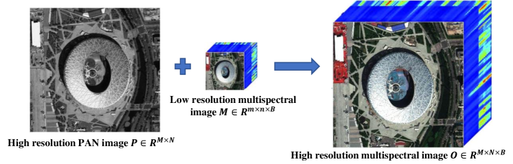
Figure 1: The schematic diagram of pansharpening.

The CS-based approaches rely on the concept of the projection of the LRMS image into a new domain, where the spatial information can be easily separated into a component, usually called the intensity component. Then, the PAN image can be substituted with the intensity component. Representative methods include principal component analysis (PCA) (Shah, Younan, and King 2008), intensity–hue-saturation (Carper, Lillesand, and Kiefer 1990), and Gram–Schmidt spectral sharpening appoach (Laben and Brower 2000). The CS-based methods are easy to implement and can approximate the resolution of the HRMS image in the spatial domain but result in spectral distortion (Vivone et al. 2014). To alleviate this issue, some improved methods have been presented, such as the spatial-detail approach with the band-dependent property (BDSD) (Garzelli, Nencini, and Capobianco 2007), the robust version of BDSD approach (Vivone 2019), and the adaptive CS approach with partial replacement (Choi, Yu, and Kim 2010).

The MRA-based methods depend on injecting the spatial details captured by decomposing the PAN image in a multiresolution way to the LRMS image. This type of method can preserve spectral information but bring in spatial distortion. Typical methods include the intensity modulation with smooth filter (Liu 2000), the additive wavelet luminance proportional (AWLP) (Otazu et al. 2005), the Laplacian pyramid-based methods (Restaino et al. 2019; Vivone, Marano, and Chanussot 2020; Vivone, Restaino, and Chanussot 2018).

The VO-based techniques are adopted by formulating pansharpening as a variational optimization problem, which contains elegant mathematical derivation but often suffers from a high computational burden. Typical approaches include the Bayesian methods (Wang et al. 2018), variational approaches (Fang et al. 2013a, b; Deng et al. 2018; Deng, Feng, and Tai 2019; Fu et al. 2019; Tian et al. 2021), and compressed sensing approaches (Li and Yang 2010).

Recently, the DL-based approaches have been extensively studied, and this type of method directly learns the mapping from LRMS and PAN to HRMS by some stacked network architectures. For example, Huang et al. (Huang et al. 2015) firstly proposed a stacked modified sparse denoising autoencoder (S-MSDA) to train the relationship between high-resolution (HR) and low-resolution (LR) image patches. Masi et al. (Masi et al. 2016) designed a simple and effective three-layer convolutional neural network (CNN) for the pansharpening problem. Further, a deeper network based on the ResNet is built in (Yang et al. 2017; Fu et al. 2020) by focusing on the spectral and spatial preservations. A multiple-scale and multiple-depth CNN is proposed in (Yuan et al. 2018). Later, He et al. (He et al. 2019) proposed a network by combining the detail injection strategy with the CNN. Lately, Xie et al. (Xie et al. 2020b) designed a generative adversarial network (GAN) based network. Zhou et al. (Zhou, Liu, and Wang 2021) proposed an unsupervised generative multiadversarial network. Similarly, Deng et al. (Deng et al. 2020) devised a detailed injection-based network by deriving from the CS and MRA frameworks. More recently, Yang et al. (Yang et al. 2021) proposed a dual-stream CNN with residual information enhancement. Zhang et al. (Zhang and Ma 2021) developed a residual learning network based on gradient transformation prior. However, the network architectures of these DL-based approaches are empirically designed by stacking some network modules, and thus the entire architectures can be seen as black-box mechanisms, and the role of different modules in these networks is difficult to analyze and understand. To alleviate this issue, some attempts by combining the model-based methodology with the deep learning method have been made. For example, Xie et al. (Xie et al. 2020a) designed an interpretable deep network for multispectral and hyperspectral image fusion. Dong et al. (Dong et al. 2021) proposed a model-guided deep network for hyperspectral image super-resolution. Yin et al. (Yin 2021) and Cao et al. (Cao et al. 2021) proposed two model-driven deep networks for pansharpening.

In this paper, we keep exploring in this direction and propose a novel deep network, dubbed as Proximal PanNet, for the pansharpening problem by combining the model-based methodology with the deep learning method. Firstly, we propose a new observation model for pansharpening using the convolutional sparse coding (CSC) technique. Specifically, we model the PAN and MS image separately using the CSC with two types of features, i.e., common features and unique features. The two features are based on two observations. One is that the PAN and MS images capture the same scene, they thus share some common features, and the other one is that the two images are generated by different sensors equipped on the satellite, they thus contain their unique features. Therefore, to generate a better fused HRMS image, we need to capture the common and unique features from the two images, and then reconstruct the HRMS image using both features. Secondly, we reformulate the observation model into an optimization problem and add implicit regularizations modeling priors on both common and unique features. Thirdly, we design a proximal gradient algorithm to solve this optimization model, and unfold the iterative algorithm into a deep network, where each module corresponds to a specific operation of the iterative algorithm. The proximal operators are approximated by the convolutional neural network. Therefore, each module of the unfolded network can be clearly interpreted. Finally, all the learnable modules can be automatically learned end-to-end, and thus the hyperparameter selection can be avoided. Experimental results show the superiority of our network both quantitatively and qualitatively comparing with other state-of-the-art methods.

Proposed Model

In this section, a new pansharpening model is firstly proposed. Then, a proximal gradient algorithm is derived to optimize this model. Finally, the algorithm is further unfolded into a deep neural network.

Proposed Model for Pansharpening

The pansharpening model is proposed based on the following observations. Firstly, since both the LRMS image $\textbf{M}\in\mathbb{R}^{m\times n\times B}$ and the PAN image $\textbf{P}\in\mathbb{R}^{M\times N}$ are captured in the same scene, they should share some common features. Secondly, since the two images are acquired by different sensors in the satellite, each image thus has its unique feature. Additionally, we also assume that the information underlying both the LRMS image and the PAN image are beneficial to estimate the HRMS image $\textbf{O}\in\mathbb{R}^{M\times N\times B}$. Therefore, we firstly extract these effective features from both images, and then fuse these features to generate the HRMS image O. To extract the features from both images, we adopt the CSC technique (Deng and Dragotti 2020; Li et al. 2021) to model the PAN and LRMS images separately.

Specifically, our new model is defined as follows:

$$\mathbf{P} = \sum_{k=1}^{K}\mathbf{D}_{k}^{c}\otimes\mathbf{C}_{k}+\sum_{k=1}^{K}\mathbf{D}_{k}^{u}\otimes\mathbf{U}_{k},$$ (1)

$$\tilde{\mathbf{M}} = \sum_{k=1}^{K}\mathbf{H}_{k}^{c}\otimes\mathbf{C}_{k}+\sum_{k=1}^{K}\mathbf{H}_{k}^{v}\otimes\mathbf{V}_{k},$$ (2)

where $\tilde{\textbf{M}}\in\mathbb{R}^{M\times N\times B}$ is the upsampled version of the LRMS image M using the polynomial kernel technique (Aiazzi et al. 2002), $\otimes$ is the convolutional operation, $\mathbf{D}_{k}^{c}\in\mathbb{R}^{s\times s}$ and $\mathbf{H}_{k}^{c}\in\mathbb{R}^{s\times s\times B}$ denote the common filter for both images; $\mathbf{D}_{k}^{u}\in\mathbb{R}^{s\times s}$ and $\mathbf{H}_{k}^{v}\in\mathbb{R}^{s\times s\times B}$ represent the separate filters of both images; $\mathbf{C}_{k}\in\mathbb{R}^{M\times N}$ denotes the shared common features, and $\mathbf{U}_{k}\in\mathbb{R}^{M\times N}$ and $\mathbf{V}_{k}\in\mathbb{R}^{M\times N}$ are unique features of HRMS image and LRHS image, respectively. Then, the HRMS image $\mathbf{O}\in\mathbb{R}^{M\times N\times B}$ can be generated by fusing these features as follows:

$$\mathbf{O}\!=\!\sum_{k=1}^{K}\mathbf{G}_{k}^{c}\!\otimes\!\mathbf{C}_{k}\!+\!\sum_{k=1}^{K}\mathbf{G}_{k}^{u}\!\otimes\!\mathbf{U}_{k}\!+\!\sum_{k=1}^{K}\mathbf{G}_{k}^{v}\!\otimes\!\mathbf{V}_{k},$$ (3)

where $\mathbf{G}_{k}^{c}\in\mathbb{R}^{s\times s\times B}$ represents the common filter, $\mathbf{G}_{k}^{u}\in\mathbb{R}^{s\times s\times B}$ and $\mathbf{G}_{k}^{v}\in\mathbb{R}^{s\times s\times B}$ denote the unique filters concerning the features of both images. To make the notations clear, we denote $\mathbf{C}=\{\mathbf{C}_{k}\}_{k=1}^{K}\in\mathbb{R}^{M\times N\times K}$, $\mathbf{U}=\{\mathbf{U}_{k}\}_{k=1}^{K}\in\mathbb{R}^{M\times N\times K}$, and $\mathbf{V}=\{\mathbf{V}_{k}\}_{k=1}^{K}\in\mathbb{R}^{M\times N\times K}$.

In the following, we assume that all the filters are known. Therefore, to obtain the fused HRMS image O, we need to calculate $\mathbf{C}$, $\mathbf{U}$, and $\mathbf{V}$ as follows:

$$\begin{split}\min_{\mathbf{C},\mathbf{U},\mathbf{V}}\frac{1}{2}||\mathbf{P}-\sum_{k=1}^{K}\mathbf{D}_{k}^{c}\otimes\mathbf{C}_{k}-\sum_{k=1}^{K}\mathbf{D}_{k}^{u}\otimes\mathbf{U}_{k}||_{F}^{2}\\ +~{}\frac{1}{2}||\tilde{\mathbf{M}}-\sum_{k=1}^{K}\mathbf{H}_{k}^{c}\otimes\mathbf{C}_{k}-\sum_{k=1}^{K}\mathbf{H}_{k}^{v}\otimes\mathbf{V}_{k}||_{F}^{2}\\ +\lambda_{1}f_{1}(\mathbf{U})+\lambda_{2}f_{2}(\mathbf{V})+\lambda_{3}f_{3}(\mathbf{C}),\end{split}$$ (4)

where $\lambda_{1},\lambda_{2}$, and $\lambda_{3}$ are the trade-off parameters. $f_{1}(\cdot),f_{2}(\cdot)$, and $f_{3}(\cdot)$ are the regularization terms modeling the priors on $\mathbf{U}$, $\mathbf{V}$, and $\mathbf{C}$, respectively.

Model Optimization

To solve the problem, we adopt the alternate optimization algorithm to alternately update each variable with other variables fixed, which leads to the three sub-problems:

$$\begin{split}\mathbf{U}^{(t)}\!=\!\arg\!\min_{\mathbf{U}}&||\mathbf{P}\!-\!\sum_{k=1}^{K}\!\mathbf{D}_{k}^{c}\!\otimes\!\mathbf{C}_{k}^{(t-1)}\!-\!\sum_{k=1}^{K}\!\mathbf{D}_{k}^{u}\!\otimes\!\mathbf{U}_{k}||_{F}^{2}\!\\ &+\!\lambda_{1}f_{1}(\mathbf{U}),\end{split}$$ (5)

$$\begin{split}\mathbf{V}^{(t)}\!=\!\arg\!\min_{\mathbf{V}}&||\tilde{\mathbf{M}}\!\!-\!\!\sum_{k=1}^{K}\mathbf{H}_{k}^{c}\!\!\otimes\!\!\mathbf{C}_{k}^{(t-1)}\!\!-\!\!\sum_{k=1}^{K}\mathbf{H}_{k}^{v}\!\!\otimes\!\!\mathbf{V}_{k}||_{F}^{2}\!\\ &+\!\lambda_{2}f_{2}(\mathbf{V}),\end{split}$$ (6)

$$\begin{split}&\mathbf{C}^{(t)}\!=\!\arg\!\min_{\mathbf{C}}||\mathbf{P}\!\!-\!\!\sum_{k=1}^{K}\mathbf{D}_{k}^{c}\!\otimes\!\mathbf{C}_{k}\!-\!\sum_{k=1}^{K}\mathbf{D}_{k}^{u}\!\otimes\!\mathbf{U}_{k}^{(t)}||_{F}^{2}\\ &\!+\!||\tilde{\mathbf{M}}\!-\!\sum_{k=1}^{K}\mathbf{H}_{k}^{c}\!\otimes\!\mathbf{C}_{k}\!\!-\!\!\!\sum_{k=1}^{K}\mathbf{H}_{k}^{v}\!\otimes\!\mathbf{V}_{k}^{(t)}||_{F}^{2}\!+\!\lambda_{3}f_{3}(\mathbf{C}).\end{split}$$ (7)

Next, we introduce the optimization for each sub-problem.

$\mathbf{U}-$subproblem

Instead of directly optimizing the objective (5), we first adopt the quadratic function to approximate the objective function, which is expressed as:

$$\begin{split}\mathbf{U}^{(t)}\!=\!\arg\min_{\mathbf{U}}g\left(\mathbf{U}^{(t-1)}\right)\!+\!\frac{1}{2\eta_{1}}||\mathbf{U}-\mathbf{U}^{(t-1)}||_{F}^{2}\\ \!+\!\left<\nabla g(\mathbf{U}^{(t-1)}),\mathbf{U}\!-\!\mathbf{U}^{(t-1)}\right>\!+\!\lambda_{1}f_{1}(\mathbf{U}),\end{split}$$ (8)

where

$$g\left(\mathbf{U}^{(t\!-\!1)}\right)\!\!\!=\!\!||\mathbf{P}\!\!-\!\!\!\sum_{k=1}^{K}\!\mathbf{D}_{k}^{c}\!\otimes\!\mathbf{C}_{k}^{(t\!-\!1)}\!\!-\!\!\!\sum_{k=1}^{K}\!\mathbf{D}_{k}^{u}\!\otimes\!\mathbf{U}_{k}^{(t\!-\!1)}\!\!||_{F}^{2},$$ (9)

$$\nabla g(\mathbf{U}^{(t\!-\!1)})\!\!=\!\!\mathbf{D}^{u}\!\otimes^{\dagger}\!\left(\sum_{k=1}^{K}\!\mathbf{D}_{k}^{c}\!\otimes\!\mathbf{C}_{k}^{(t\!-\!1)}\!\!+\!\!\sum_{k=1}^{K}\!\mathbf{D}_{k}^{u}\!\otimes\!\mathbf{U}_{k}^{(t\!-\!1)}\!\!-\!\!\mathbf{P}\right),$$ (10)

$\nabla(\cdot)$ is gradient operator, $\eta_{1}$ is the step size, $\mathbf{D}^{u}\in\mathbb{R}^{s\times s\times K\times 1}$ is a 4$-$D tensor stacked by all $\mathbf{D}_{k}^{u}$, and $\otimes^{\dagger}$ denotes the transposed convolution. By a simple mathematical derivation, Eq. (8) can be equivalent to

$$\begin{split}\mathbf{U}^{(t)}=\arg\min_{\mathbf{U}}&\frac{1}{2}||\mathbf{U}-(\mathbf{U}^{(t-1)}-\eta_{1}\nabla g(\mathbf{U}^{(t-1)}))||_{F}^{2}\\ &+\eta_{1}\lambda_{1}f_{1}(\mathbf{U}).\end{split}$$ (11)

Eq.(11) can then be optimized by the general proximal operator (Beck and Teboulle 2009), which is defined as

$$\mathbf{U}^{(t)}=prox_{\eta_{1}\lambda_{1}}\left(\mathbf{U}^{(t-1)}-\eta_{1}\nabla g(\mathbf{U}^{(t-1)})\right),$$ (12)

where $prox_{\eta_{1}\lambda_{1}}(\cdot)$ is the proximal operator related to $f_{1}(\cdot)$. To alleviate the limitation of human designed regularizers, we adopt the deep CNNs to automatically learn the prior from the data, which will be discussed in detail in the next subsection.

$\mathbf{V}-$subproblem

For the updating of $\mathbf{V}$, we adopt a similar strategy. Firstly, the quadratic approximation of (6) with respect to $\mathbf{V}$ is defined as:

$$\begin{split}\mathbf{V}^{(t)}=\arg\min_{\mathbf{V}}h\left(\mathbf{V}^{(t-1)}\right)+\frac{1}{2\eta_{2}}||\mathbf{V}-\mathbf{V}^{(t-1)}||_{F}^{2}\\ +\left<\nabla h(\mathbf{V}^{(t-1)}),\mathbf{V}-\mathbf{V}^{(t-1)}\right>+\lambda_{2}f_{2}(\mathbf{V}),\end{split}$$ (13)

where

$$h\left(\mathbf{V}^{(t-1)}\right)\!\!=\!\!||\tilde{\mathbf{M}}\!\!-\!\!\sum_{k=1}^{K}\!\mathbf{H}_{k}^{c}\!\otimes\!\mathbf{C}_{k}^{(t-1)}\!\!-\!\!\sum_{k=1}^{K}\!\mathbf{H}_{k}^{v}\!\otimes\!\mathbf{V}_{k}^{(t-1)}||_{F}^{2},$$ (14)

$$\nabla h(\mathbf{V}^{(t-1)})\!\!=\!\!\mathbf{H}^{v}\!\!\otimes^{\dagger}\!\!\left(\sum_{k=1}^{K}\!\mathbf{H}_{k}^{c}\!\!\otimes\!\!\mathbf{C}_{k}^{(t\!-\!1)}\!\!+\!\!\sum_{k=1}^{K}\!\mathbf{H}_{k}^{v}\!\otimes\!\mathbf{V}_{k}^{(t\!-\!1)}\!\!-\!\!\tilde{\mathbf{M}}\right),$$ (15)

$\eta_{2}$ is the step size, and $\mathbf{H}^{v}\in\mathbb{R}^{s\times s\times K\times B}$ is a 4$-$D tensor stacked by all $\mathbf{H}_{k}^{v}$. Further, Eq. (13) can be equivlently formulated as

$$\begin{split}\mathbf{V}^{(t)}=\arg\min_{\mathbf{V}}&\frac{1}{2}||\mathbf{V}-(\mathbf{V}^{(t-1)}-\eta_{2}\nabla h(\mathbf{V}^{(t-1)}))||_{F}^{2}\\ &+\eta_{2}\lambda_{2}f_{2}(\mathbf{V}),\end{split}$$ (16)

Then, Eq.(16) can also be solved by

$$\mathbf{V}^{(t)}=prox_{\eta_{2}\lambda_{2}}\left(\mathbf{V}^{(t-1)}-\eta_{2}\nabla h(\mathbf{V}^{(t-1)})\right),$$ (17)

where $prox_{\eta_{2}\lambda_{2}}(\cdot)$ is the proximal operator related to $f_{2}(\cdot)$.

$\mathbf{C}-$subproblem

Eq. (7) can be re-written as:

$$\begin{split}\mathbf{C}^{(t)}&=\arg\min_{\mathbf{C}}||\hat{\mathbf{P}}-\sum_{k=1}^{K}\mathbf{D}_{k}^{c}\otimes\mathbf{C}_{k}||_{F}^{2}\\ &+||\hat{\mathbf{M}}-\sum_{k=1}^{K}\mathbf{H}_{k}^{c}\otimes\mathbf{C}_{k}||_{F}^{2}+\lambda_{3}f_{3}(\mathbf{C}),\end{split}$$ (18)

where $\hat{\mathbf{P}}=\mathbf{P}-\sum_{k=1}^{K}\mathbf{D}_{k}^{u}\otimes\mathbf{U}_{k}^{(t)}$ and $\hat{\mathbf{M}}=\tilde{\mathbf{M}}-\sum_{k=1}^{K}\mathbf{H}_{k}^{v}\otimes\mathbf{V}_{k}^{(t)}$. Further, Eq. (18) can be expressed as:

$$\mathbf{C}^{(t)}\!=\!\arg\min_{\mathbf{C}}||\mathbf{N}\!\!-\!\!\sum_{k=1}^{K}\mathbf{L}_{k}^{c}\otimes\mathbf{C}_{k}||_{F}^{2}\!+\!\lambda_{3}f_{3}(\mathbf{C}),$$ (19)

where $\mathbf{N}\in\mathbb{R}^{M\times N\times(B+1)}$ is the concatenation of $\hat{\mathbf{P}}$ and $\hat{\mathbf{M}}$, and $\mathbf{L}_{k}^{c}\in\mathbb{R}^{s\times s\times(B+1)}$ is the concatenation of $\mathbf{D}_{k}^{c}$ and $\mathbf{H}_{k}^{c}$. Eq. (19) can then be solved by the same way as optimizing $\mathbf{U}$ and $\mathbf{V}$. More specifically, we first derive the quadratic approximation of Eq. (19) with respect to $\mathbf{C}$ as follows:

$$\begin{split}\mathbf{C}^{(t)}=\arg\min_{\mathbf{C}}l\left(\mathbf{C}^{(t-1)}\right)+\frac{1}{2\eta_{3}}||\mathbf{C}-\mathbf{C}^{(t-1)}||_{F}^{2}\\ +\left<\nabla l(\mathbf{C}^{(t-1)}),\mathbf{C}-\mathbf{C}^{(t-1)}\right>+\lambda_{3}f_{3}(\mathbf{C}),\end{split}$$ (20)

where

$$l\left(\mathbf{C}^{(t-1)}\right)\!\! = \!\!||\mathbf{N}\!\!-\!\!\sum_{k=1}^{K}\!\mathbf{L}_{k}^{c}\!\otimes\!\mathbf{C}_{k}^{(t-1)}||_{F}^{2},$$ (21)

$$\nabla l(\mathbf{C}^{(t-1)})\!\! = \!\!\mathbf{L}^{c}\!\otimes^{\dagger}\!\left(\sum_{k=1}^{K}\!\mathbf{L}_{k}^{c}\!\otimes\!\mathbf{C}_{k}^{(t-1)}\!-\!\mathbf{N}\right),$$ (22)

$\eta_{3}$ is the step size, and $\mathbf{L}^{c}\in\mathbb{R}^{s\times s\times K\times(B+1)}$ is a 4$-$D tensor stacked by all $\mathbf{L}_{k}^{c}$. Further, Eq. (20) can be rewritten as

$$\begin{split}\mathbf{C}^{(t)}=\arg\min_{\mathbf{C}}&\frac{1}{2}||\mathbf{C}-(\mathbf{C}^{(t-1)}-\eta_{3}\nabla l(\mathbf{C}^{(t-1)}))||_{F}^{2}\\ &+\eta_{3}\lambda_{3}f_{3}(\mathbf{C}).\end{split}$$ (23)

Finally, Eq.(23) can be solved as

$$\mathbf{C}^{(t)}=prox_{\eta_{3}\lambda_{3}}\left(\mathbf{C}^{(t-1)}-\eta_{3}\nabla l(\mathbf{C}^{(t-1)})\right),$$ (24)

where $prox_{\eta_{3}\lambda_{3}}(\cdot)$ is the proximal operator related to $f_{3}(\cdot)$.

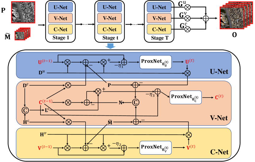
Figure 2: The overall architecture of our proposed unfolding network for pansharpening. This network is composed of $T$ stages shown at the top, and each stage contains three sub-networks (i.e., U-Net, V-Net, and C-net). The detailed network architectures of the three sub-networks in the stage $t$ are shown at the bottom. $\otimes$ and $\oplus$ represent the convolutional operation and the element-wise addition, respectively.

Proximal PanNet

Based on the iterative algorithm, we build a deep network shown in the top row of Fig. 2. This network contains $T$ stages corresponding to $T$ iterations of the iterative algorithm for solving Eq. (4). Each stage takes the outputs of the previous stage $\mathbf{U}^{(t-1)}$, $\mathbf{V}^{(t-1)}$ and $\mathbf{C}^{(t-1)}$ as the inputs and produces the updates $\mathbf{U}^{(t)}$, $\mathbf{V}^{(t)}$ and $\mathbf{C}^{(t)}$.

As shown in Eq. (12), (17) and (24), the three proximal operators ${\rm{pro}}{{\rm{x}}_{{\eta_{1}}{\lambda_{1}}}}(\cdot)$, ${\rm{pro}}{{\rm{x}}_{{\eta_{2}}{\lambda_{2}}}}(\cdot)$, and ${\rm{pro}}{{\rm{x}}_{{\eta_{3}}{\lambda_{3}}}}(\cdot)$ play a key role in the algorithm. To update each variable, classical methods usually design hand-crafted priors which make the proximal operators be closed form. However, due to the limited representation abilities, human-designed priors cannot always achieve the expected effect. Therefore, we utilize convolutional neural networks to explore prior for $\mathbf{U}$, $\mathbf{V}$ and $\mathbf{C}$, namely learning their corresponding proximal operators ${\rm{pro}}{{\rm{x}}_{{\eta_{1}}{\lambda_{1}}}}(\cdot)$, ${\rm{pro}}{{\rm{x}}_{{\eta_{2}}{\lambda_{2}}}}(\cdot)$, and ${\rm{pro}}{{\rm{x}}_{{\eta_{3}}{\lambda_{3}}}}(\cdot)$ for updating $\mathbf{U}^{(t)}$, $\mathbf{V}^{(t)}$, and $\mathbf{C}^{(t)}$ in each stage $t$.

Network design

Our network is designed as several stages, and each stage updates $\mathbf{U}$, $\mathbf{V}$ and $\mathbf{C}$ in a cascaded manner. At stage $t$, $\mathbf{U}^{(t)}$ is updated using $\mathbf{P}$, $\mathbf{U}^{(t-1)}$, and $\mathbf{C}^{(t-1)}$ by the following sub-steps:

$$\begin{split}\mathbf{U-Net}:\left\{\begin{array}[]{ll}&\!\!\!\!\!\mathbf{P}_{c}^{(t-1)}=\sum_{k=1}^{K}\mathbf{D}_{k}^{c}\otimes\mathbf{C}_{k}^{(t-1)},\\ &\!\!\!\!\!\mathbf{P}_{u}^{(t-1)}=\sum_{k=1}^{K}\mathbf{D}_{k}^{u}\otimes\mathbf{U}_{k}^{(t-1)},\\ &\!\!\!\!\!\mathbf{\varepsilon}_{P}^{(t-1)}=\mathbf{P}_{c}^{(t-1)}+\mathbf{P}_{u}^{(t-1)}-\mathbf{P},\\ &\!\!\!\!\!\nabla g^{(t-1)}=\mathbf{D}^{u}\otimes^{\dagger}\mathbf{\varepsilon}_{P}^{(t-1)},\\ &\!\!\!\!\!\mathbf{U}^{(t-0.5)}=\mathbf{U}^{(t-1)}-\eta_{1}\nabla g^{(t-1)},\\ &\!\!\!\!\!\mathbf{U}^{(t)}={\rm{proxNe}}{{\rm{t}}_{\Theta_{\bf{U}}^{(t)}}}\left(\mathbf{U}^{(t-0.5)}\right).\end{array}\right.\end{split}$$ (25)

Each step is unfolded into one module of the U-Net shown in Figure 2. Then, $\mathbf{V}^{(t)}$ is updated by $\tilde{\mathbf{M}}$, $\mathbf{V}^{(t-1)}$, and $\mathbf{C}^{(t-1)}$:

$$\begin{split}\mathbf{V-Net}:\left\{\begin{array}[]{ll}&\!\!\!\!\!\mathbf{M}_{c}^{(t-1)}=\sum_{k=1}^{K}\mathbf{H}_{k}^{c}\otimes\mathbf{C}_{k}^{(t-1)},\\ &\!\!\!\!\!\mathbf{M}_{v}^{(t-1)}=\sum_{k=1}^{K}\mathbf{H}_{k}^{v}\otimes\mathbf{V}_{k}^{(t-1)},\\ &\!\!\!\!\!\mathbf{\varepsilon}_{M}^{(t-1)}=\mathbf{M}_{c}^{(t-1)}+\mathbf{\textsc{M}}_{v}^{(t-1)}-\tilde{\mathbf{M}},\\ &\!\!\!\!\!\nabla h^{(t-1)}=\mathbf{H}^{v}\otimes^{\dagger}\mathbf{\varepsilon}_{M}^{(t-1)},\\ &\!\!\!\!\!\mathbf{V}^{(t-0.5)}=\mathbf{V}^{(t-1)}-\eta_{2}\nabla h^{(t-1)},\\ &\!\!\!\!\!\mathbf{V}^{(t)}={\rm{proxNe}}{{\rm{t}}_{\Theta_{\bf{V}}^{(t)}}}\left(\mathbf{V}^{(t-0.5)}\right).\end{array}\right.\end{split}$$ (26)

Similarly, each step is unfolded into one module of the V-Net as shown in Figure 2. Finally, $\mathbf{C}^{(t)}$ is updated using $\mathbf{P}$, $\tilde{\mathbf{M}}$, $\mathbf{C}^{(t-1)}$, $\mathbf{U}^{(t)}$ and $\mathbf{V}^{(t)}$:

$$\begin{split}\mathbf{C-Net}:\left\{\begin{array}[]{ll}&\!\!\!\!\!\mathbf{F}_{c}^{(t-1)}=\sum_{k=1}^{K}\mathbf{L}_{k}^{c}\otimes\mathbf{C}_{k}^{(t-1)},\\ &\!\!\!\!\!\mathbf{\varepsilon}_{C}^{(t-1)}=\mathbf{F}_{c}^{(t-1)}-\mathbf{N},\\ &\!\!\!\!\!\nabla l^{(t-1)}=\mathbf{L}^{c}\otimes^{\dagger}\mathbf{\varepsilon}_{C}^{(t-1)},\\ &\!\!\!\!\!\nabla l^{(t-0.5)}=\mathbf{C}^{(t-1)}-\eta_{3}\nabla l^{(t-1)},\\ &\!\!\!\!\!\mathbf{C}^{(t)}={\rm{proxNe}}{{\rm{t}}_{\Theta_{\bf{C}}^{(t)}}}\left(l^{(t-0.5)}\right).\end{array}\right.\end{split}$$ (27)

Similarly, each step is unfolded into one module of the C-Net as shown in Figure 2. Additionally, ${\rm{proxNe}}{{\rm{t}}_{\Theta_{\bf{U}}^{(t)}}}(\cdot)$, ${\rm{proxNe}}{{\rm{t}}_{\Theta_{\bf{V}}^{(t)}}}(\cdot)$ and ${\rm{proxNe}}{{\rm{t}}_{\Theta_{\bf{C}}^{(t)}}}(\cdot)$ are all ResNet (He et al. 2016) with 3 ResBlocks, which are used to approximate the three proximal operators, and ${\Theta_{\bf{U}}^{(t)}}$, ${\Theta_{\bf{V}}^{(t)}}$, and ${\Theta_{\bf{C}}^{(t)}}$ are the corresponding network parameters at the $t^{th}$ stage. Besides, ${\Theta_{\bf{U}}^{(t)}}$, ${\Theta_{\bf{V}}^{(t)}}$, and ${\Theta_{\bf{C}}^{(t)}}$ are the parameters of the three ResNets at the $t^{th}$ stage. Note that all the network parameters can be end-to-end learned from training data, including $\{\Theta_{\bf{U}}^{(t)},\Theta_{\bf{V}}^{(t)},\Theta_{\bf{C}}^{(t)}\}_{t=1}^{T}$, $\mathbf{D}^{c}=\{\mathbf{D}^{c}_{k}\}_{k=1}^{K}$, $\mathbf{D}^{u}=\{\mathbf{D}^{u}_{k}\}_{k=1}^{K}$, $\mathbf{H}^{c}=\{\mathbf{H}^{c}_{k}\}_{k=1}^{K}$, $\mathbf{H}^{v}=\{\mathbf{H}^{v}_{k}\}_{k=1}^{K}$, $\mathbf{G}^{c}=\{\mathbf{G}^{c}_{k}\}_{k=1}^{K}$, $\mathbf{G}^{u}=\{\mathbf{G}^{u}_{k}\}_{k=1}^{K}$, $\mathbf{G}^{v}=\{\mathbf{G}^{v}_{k}\}_{k=1}^{K}$, $\eta_{1}$, $\eta_{2}$, and $\eta_{3}$. Once training finished, the testing can be shortened due to its feed-forward architecture. Note that our network shown in Figure 2 is interpretable. For example,To update $\mathbf{U}^{(t)}$ by Eq. (LABEL:eq.netU), computing $\mathbf{U}^{(t-0.5)}$ means the gradient descent, and the ${\rm{proxNe}}{{\rm{t}}_{\Theta_{\bf{U}}^{(t)}}}(\cdot)$ performs nonlinear operation on ${\bf{U}}^{(t-0.5)}$.

Network training

The loss function of our training process is defined as

$$\mathcal{L}=\sum_{j=1}^{J}||\mathbf{O}_{p}^{j}-\mathbf{O}_{g}^{j}||_{2}^{2},$$ (28)

where $\mathbf{O}_{p}^{j}$ is the predicted HRMS image of the $j^{th}$ training sample, $\mathbf{O}_{g}^{j}$ is the true HRMS image of the $j^{th}$ training sample, and $J$ is the number of training pairs. In our network, all the convolutional kernel sizes are set as 8$\times$8. The channel number of each convolution is set as 16. The stage number of our network is set as 2. We implement our network using TensorFlow on a GTX 1080Ti GPU with 12 GB memory. Additionally, we adopt the Adam algorithm, and a decayed technique to set the learning rate, i.e., decayed by 0.9 every 50 epochs with a fixed initial learning rate 0.0001. Also, the epoch number is 100, and the mini-batch size is 64.

Experiments

We conduct several experiments using data from the Worldview3 satellite. Specifically, we extract 12.5$K$ image pairs from the image of Worldview3, and each image pair contains one PAN image (64$\times$64), one MS image (16$\times$16$\times$8) and one ground truth HRMS image (64$\times$64$\times$8). We split these image pairs into 90%/10% for training/testing. The ground truth HRMS image is obtained by using the Wald’s protocol (Wald, Ranchin, and Mangolini 1997) due to its unavailability. We compare with twelve state-of-the-art methods: EXP (Aiazzi et al. 2002), GS (Laben and Brower 2000), BDSD (Garzelli, Nencini, and Capobianco 2007), BDSD-PC (Vivone 2019), PRACS (Choi, Yu, and Kim 2010), AWLP (Otazu et al. 2005), GLP (Restaino et al. 2019), GLP-HPM (Vivone et al. 2013), MO (Restaino et al. 2016), SRD (Vicinanza et al. 2014), PanNet (Yang et al. 2017), and Fusion-Net (Deng et al. 2020).

The performance assessment contains two cases. In the first case where the ground-truth HRMS is known, we adopt four popular reference-based indexes (Vivone et al. 2014): the Q4 (for 4 bands) and Q8 (for 8 bands), the spectral angle mapper (SAM), the relative dimensionless global error in synthesis (ERGAS), and the spatial correlation coefficient (SCC). In the second case where the ground-truth HRMS is not available, we use $D_{\lambda}$, $D_{s}$, and the quality without reference (QNR) criteria (Vivone et al. 2014).

Evaluation at Reduced Resolution

We use 90% of the image pairs to train our network and the remaining ones (1258 images) for testing. Table 1 shows the average quantitative results and standard deviation of each method. From Table 1, it can be easily observed that the DL-based methods (PanNet, Fusion-Net, and our network) perform better than the CS and MRA approaches in terms of all the indexes, which may attribute to the strong non-linear approximation ability of the deep neural network. Additionally, compared with the PanNet and Fusion-Net, our proposed network obtains better performance, which further verifies that the CSC framework has a certain advantage over the CS and MRA frameworks since the PanNet and Fusion-Net are built based on the CS and MRA frameworks while our network is built based on the proposed CSC framework. Also, our proposed network is very robust since it has almost the smallest standard deviation.

Table 1: Average quantitative results on the test dataset (Worldview3) in the reduced resolution case (1258 images).

Methods	Q8	SAM	ERGAS	SCC
EXP (Aiazzi et al. 2002)	0.6176$\pm$0.1614	5.7123$\pm$2.1141	6.7327$\pm$3.0030	0.8137$\pm$0.0694
GS (Laben and Brower 2000)	0.8100$\pm$0.1301	6.7731$\pm$2.8316	5.0358$\pm$2.3855	0.9464$\pm$0.0329
BDSD (Garzelli, Nencini, and Capobianco 2007)	0.8482$\pm$0.1274	5.3313$\pm$2.0875	4.1042$\pm$1.9688	0.9511$\pm$0.0328
BDSD-PC (Vivone 2019)	0.7555$\pm$0.1495	5.6165$\pm$2.1201	5.1517$\pm$2.2935	0.9247$\pm$0.0394
PRACS (Choi, Yu, and Kim 2010)	0.8061$\pm$0.1400	5.4778$\pm$2.0946	4.5667$\pm$1.9784	0.9281$\pm$0.0405
AWLP (Otazu et al. 2005)	0.8479$\pm$0.1193	5.3395$\pm$1.9717	4.1996$\pm$1.9093	0.9476$\pm$0.0283
GLP (Restaino et al. 2019)	0.8533$\pm$0.1206	5.1268$\pm$1.9968	4.0173$\pm$1.8510	0.9506$\pm$0.0299
GLP-HPM (Vivone et al. 2013)	0.8472$\pm$0.1246	5.2111$\pm$2.0691	4.0717$\pm$1.8874	0.9458$\pm$0.0339
MO (Restaino et al. 2016)	0.8268$\pm$0.1327	5.2453$\pm$2.0049	4.4279$\pm$1.9556	0.9396$\pm$0.0317
SRD (Vicinanza et al. 2014)	0.8324$\pm$0.1295	5.1725$\pm$2.0210	4.3116$\pm$1.9473	0.9418$\pm$0.0308
PanNet (Yang et al. 2017)	0.9074$\pm$0.1258	3.9218$\pm$1.4958	2.6352$\pm$1.1725	0.9788$\pm$0.0235
Fusion-Net (Deng et al. 2020)	0.9125$\pm$0.1220	3.8035$\pm$1.4406	2.5771$\pm$1.1607	0.9781$\pm$0.0202
Our	0.9258$\pm$0.1203	3.6421$\pm$1.4377	2.4263$\pm$1.2355	0.9850$\pm$0.0226
Ideal value	1	0	0	1

Table 2: Average quantitative results on the Tripoli dataset (Worldview3) in the reduced resolution case.

Methods	Q8	SAM	ERGAS	SCC
EXP (Aiazzi et al. 2002)	0.7032	6.7081	8.3318	0.7408
GS (Laben and Brower 2000)	0.8158	7.2060	6.8264	0.8734
BDSD (Garzelli, Nencini, and Capobianco 2007)	0.8334	6.5331	6.5594	0.8724
BDSD-PC (Vivone 2019)	0.7706	7.1170	7.1918	0.8605
PRACS (Choi, Yu, and Kim 2010)	0.8110	6.5833	6.8484	0.8584
AWLP (Otazu et al. 2005)	0.8434	6.3811	6.3808	0.8749
GLP (Restaino et al. 2019)	0.8464	6.2880	6.3224	0.8725
GLP-HPM (Vivone et al. 2013)	0.8406	6.3400	6.3929	0.8712
MO (Restaino et al. 2016)	0.8387	6.2153	6.5142	0.8748
SRD (Vicinanza et al. 2014)	0.8400	6.2484	6.3355	0.8732
PanNet (Yang et al. 2017)	0.9815	5.0513	3.6133	0.9676
Fusion-Net (Deng et al. 2020)	0.9811	4.8672	3.4753	0.9777
Our	0.9837	4.7408	3.3942	0.9809
Ideal value	1	0	0	1

Further, we conduct another experiment on one new WorldView-3 dataset (i.e., Tripoli dataset), which has never been seen in the training phase. This dataset contains one PAN image (256$\times$256), one MS image (64$\times$64$\times$8) and one true HRMS image (256$\times$256$\times$8). The quantitative results are reported in Table 2, from which we can observe that our network achieves the best performance compared with other approaches. The visual comparison shown in Figure 3 further verifies the numerical results. For better illustration, we enlarge two regions of the fused image. Specifically, it can be seen from Figure 3 that the visual effect of classical methods contain obvious blur effects, while the three DL based methods (e.g., PanNet, FusionNet, and our network) produce better fused visual results. Additionally, we show the absolute value of residuals between the true HRMS and the predicted HRMS in Figure 4, from which we can observe that the residual image of our method contains fewer details.

(a) EXP

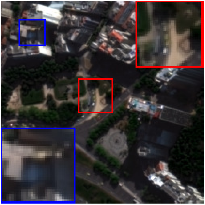
(b) GS

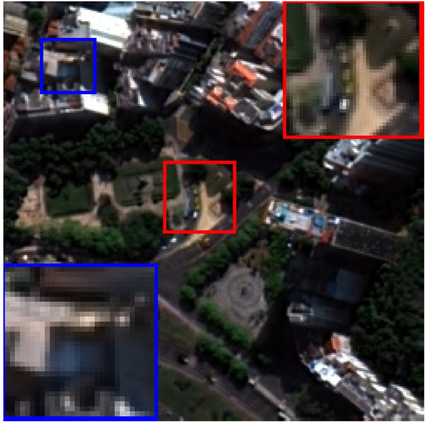
(c) BDSD

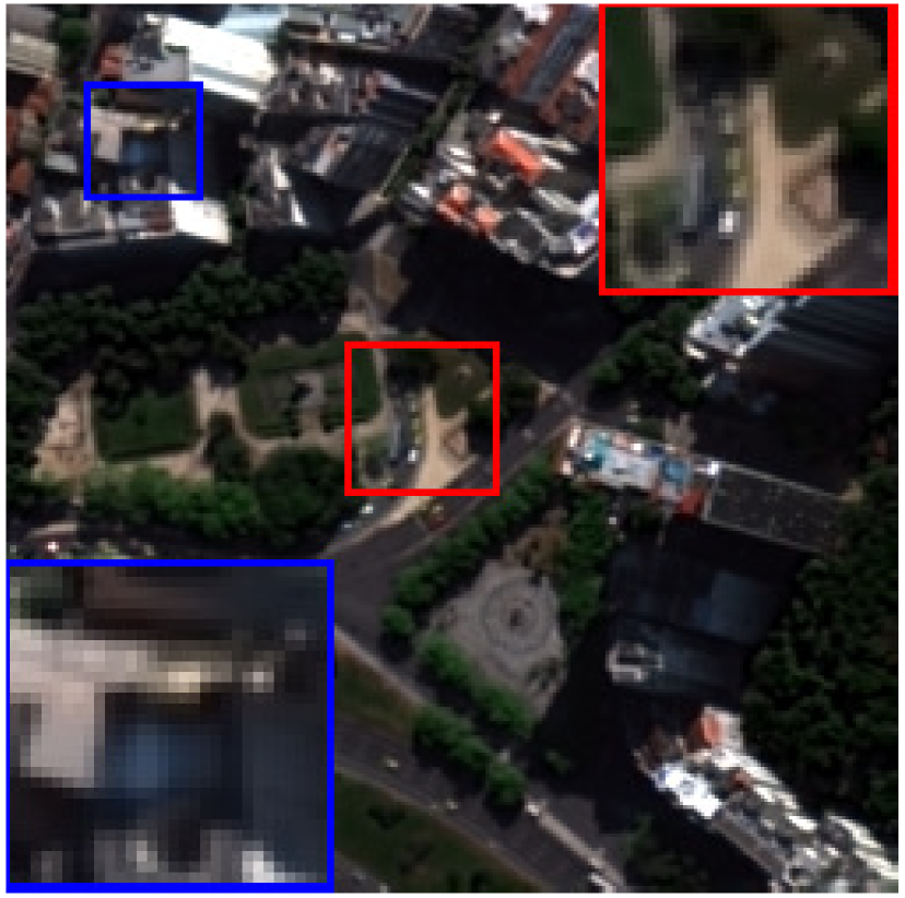
(d) BDSD-PC

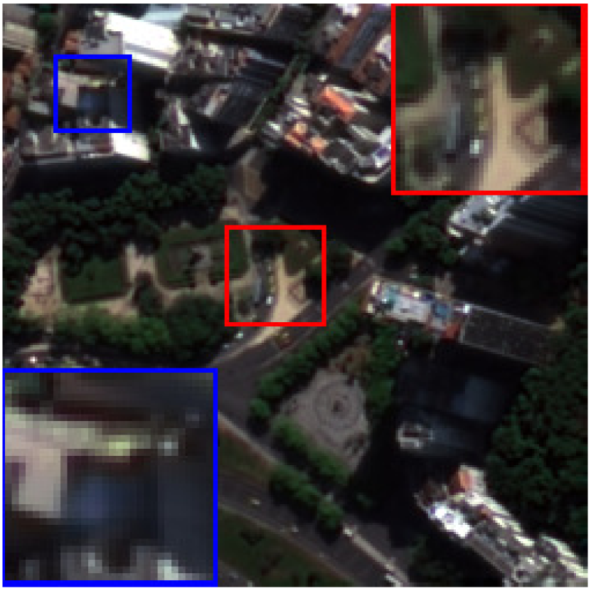
(e) PRACS

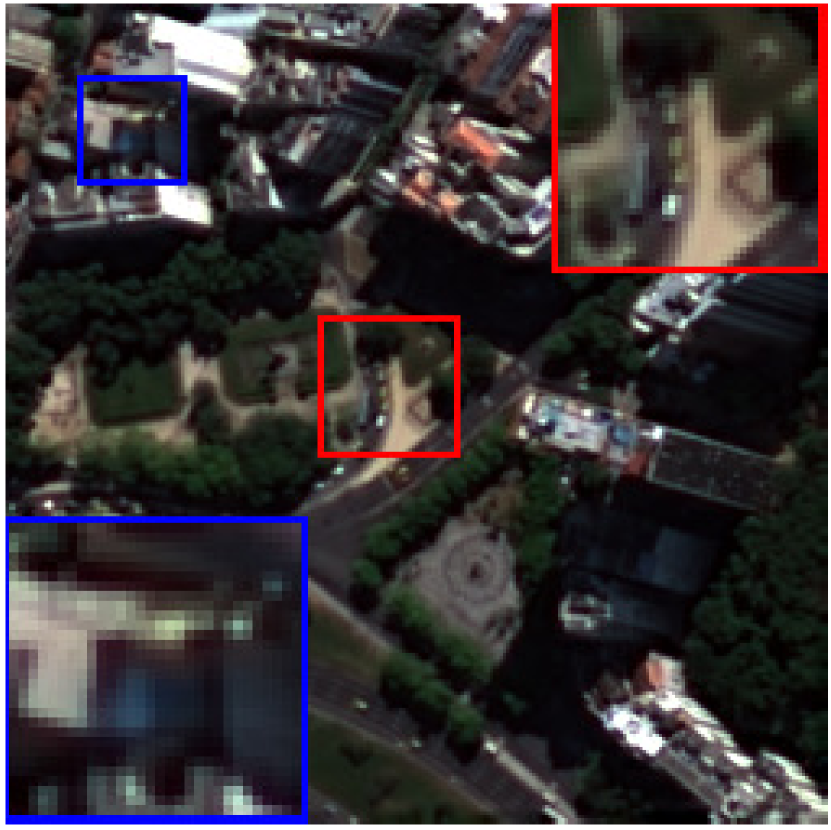
(f) AWLP

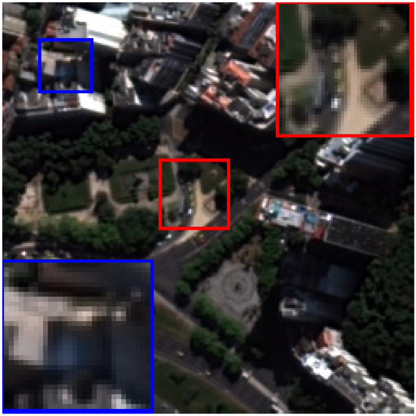
(g) GLP

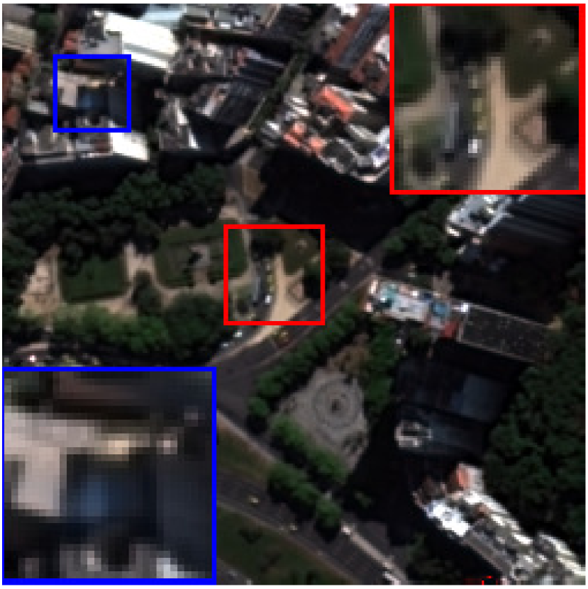
(h) GLP-HPM

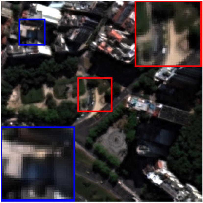
(i) MO

(j) SRD

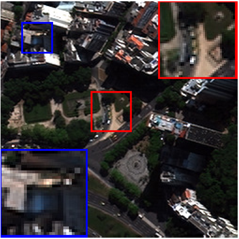
(k) PanNet

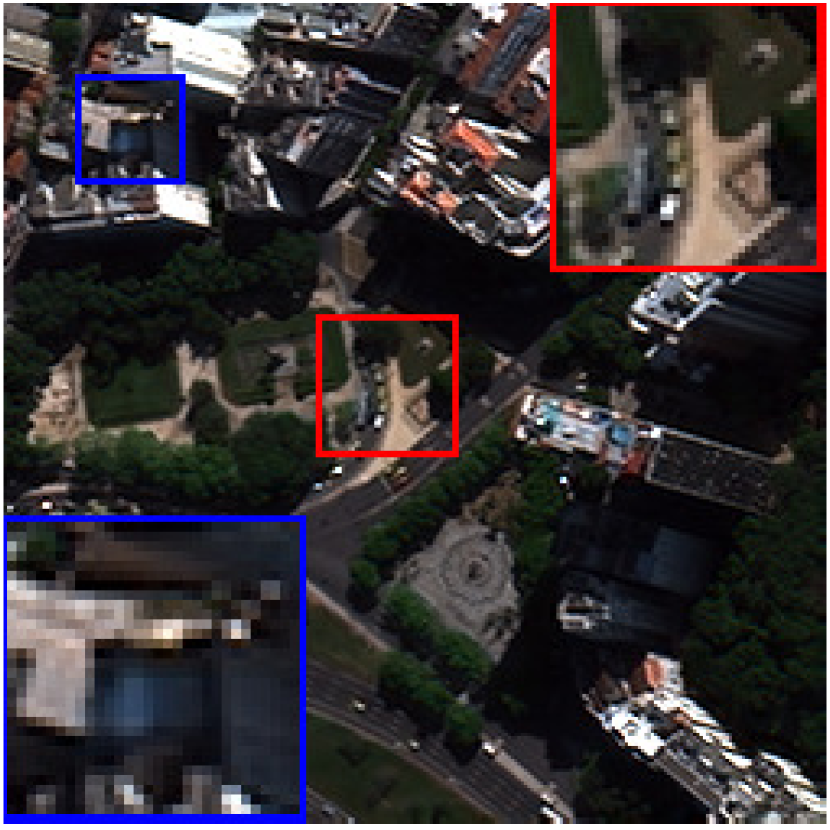
(l) Fusion-Net

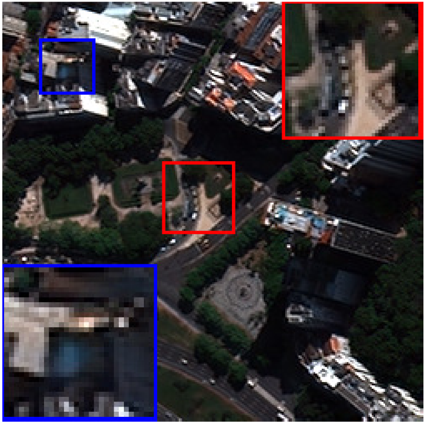
(m) Our

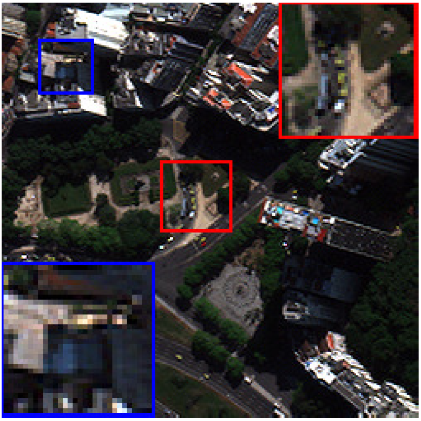
(n) GT

Figure 3: Visual comparisons of the fused HRMS image for all the methods on the Tripoli dataset.

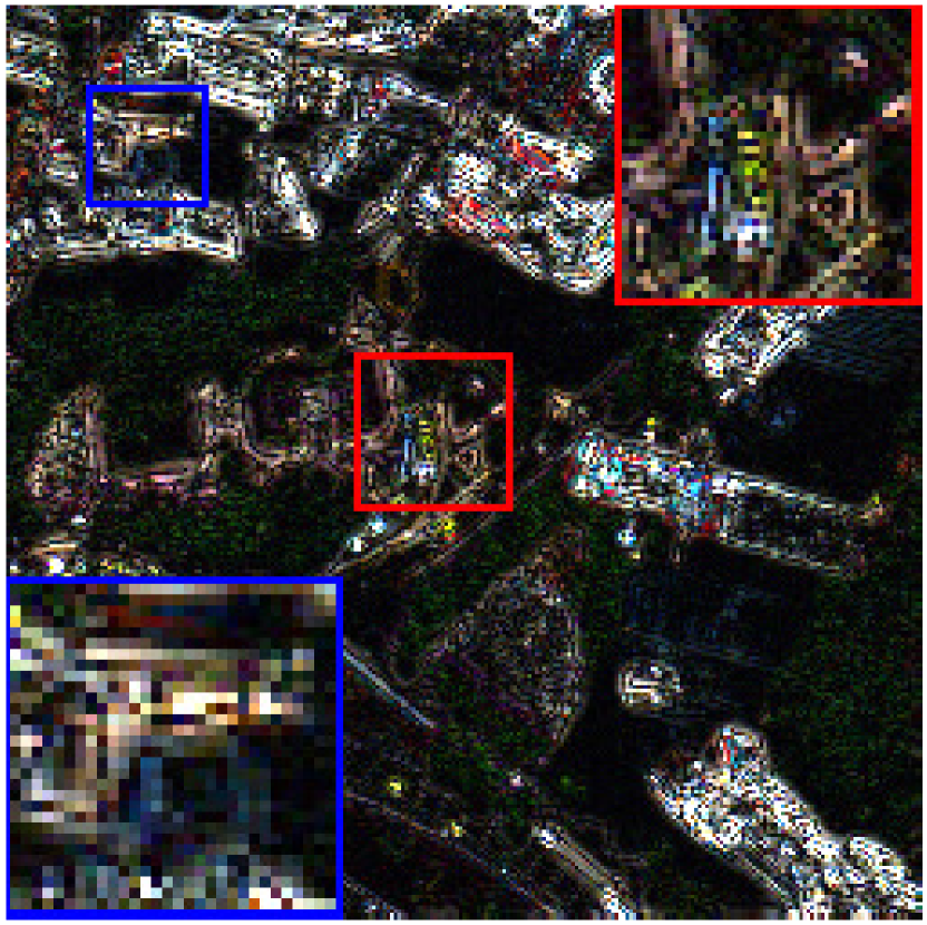
(a) EXP

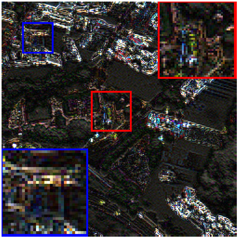
(b) GS

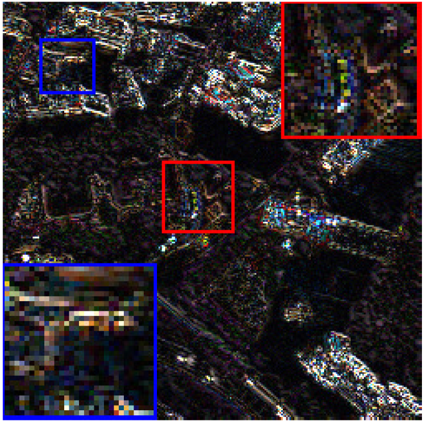
(c) BDSD

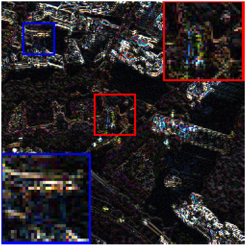
(d) BDSD-PC

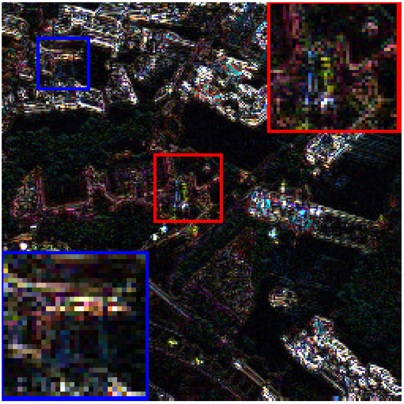
(e) PRACS

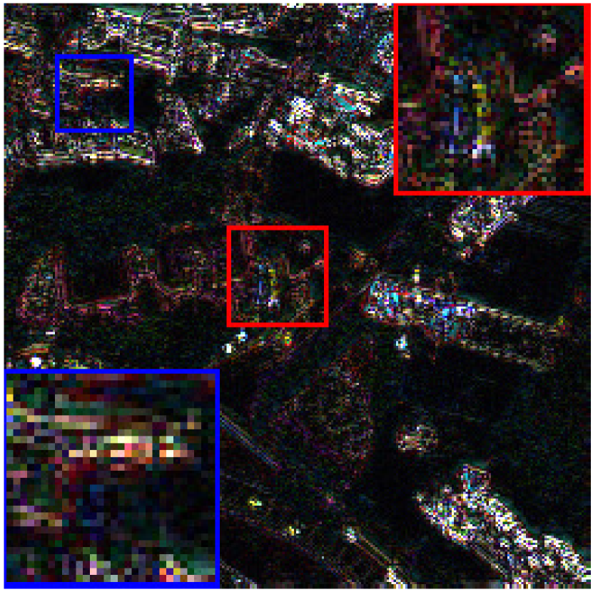
(f) AWLP

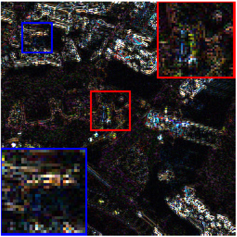
(g) GLP

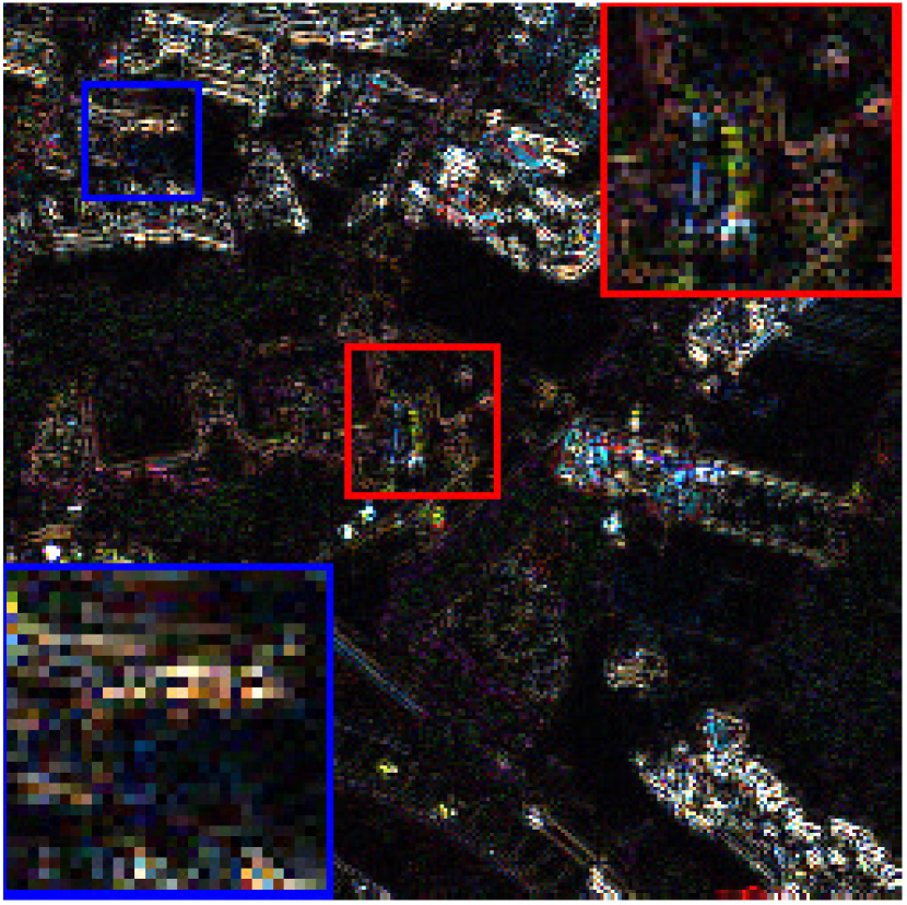
(h) GLP-HPM

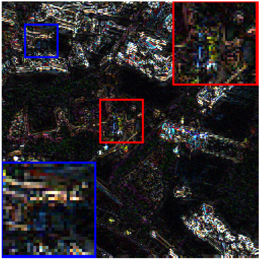
(i) MO

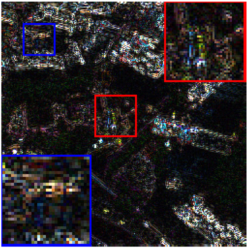
(j) SRD

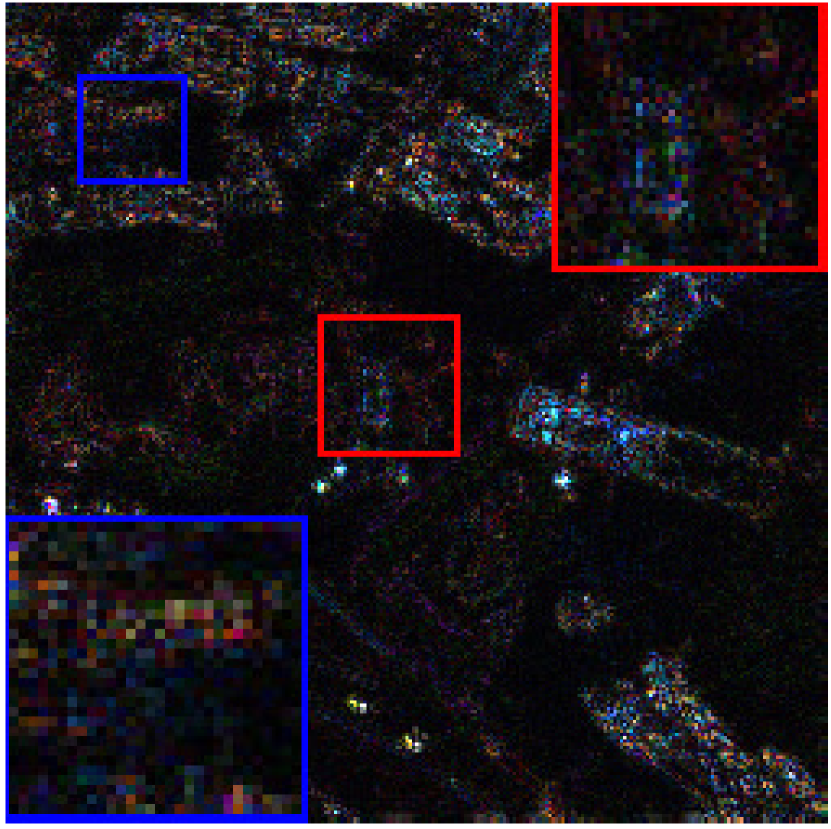
(k) PanNet

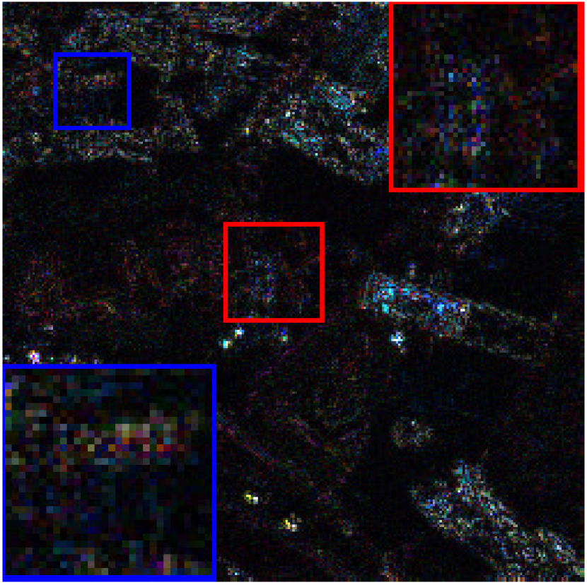
(l) Fusion-Net

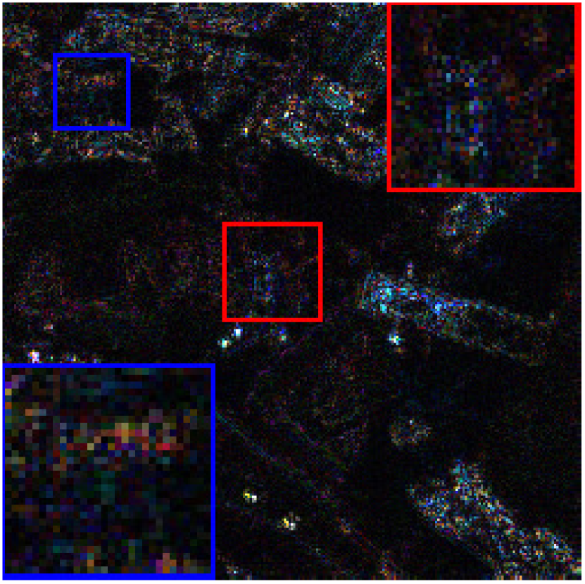
(m) Our

(n) GT

Figure 4: The absolute value of residuals between the true HRMS and the fused HRMS of Figure 3.

Evaluation at Full Resolution

This section evaluates the performance of our network in the full resolution case. We conduct this experiment on 30 image pairs from the Worldview3 satellite. Each image pair contains one PAN image (256$\times$256), and one MS image (64$\times$64$\times$8). Since the ground-truth HRMS image is not available, we thus adopt $D_{\lambda}$, $D_{s}$, and QNR (Vivone et al. 2014) as the indexes. The quantitative results are reported in Table 3. As can be seen, the DL-based methods (i.e., PanNet, Fusion-Net, and our network) perform better than other methods, which verifies the superiority of the DL methods. Among the three DL approaches, our network performs best. Additionally, we also show visual comparison of a full-resolution sample in Figure 5, which indicates that our network obtains the best visual effect both spatially and spectrally than the classical approaches, and also has a comparable visual effect with the other two DL methods.

Table 3: Average quantitative results on the WorldView-3 dataset in the full resolution case (30 samples).

Methods	$D_{\lambda}$	$D_{s}$	QNR
EXP (Aiazzi et al. 2002)	0.0104$\pm$0.0035	0.0594$\pm$0.0137	0.9276$\pm$0.0125
GS (Laben and Brower 2000)	0.0275$\pm$0.0072	0.0686$\pm$0.0190	0.9058$\pm$0.0221
BDSD (Garzelli, Nencini, and Capobianco 2007)	0.0094$\pm$0.0020	0.0429$\pm$0.0073	0.9482$\pm$0.0083
BDSD-PC (Vivone 2019)	0.0092$\pm$0.0026	0.0434$\pm$0.0078	0.9478$\pm$0.0095
PRACS (Choi, Yu, and Kim 2010)	0.0109$\pm$0.0025	0.0365$\pm$0.0071	0.9528$\pm$0.0081
AWLP (Otazu et al. 2005)	0.0161$\pm$0.0328	0.0325$\pm$0.0056	0.9518$\pm$0.0067
GLP (Restaino et al. 2019)	0.0176$\pm$0.0062	0.0385$\pm$0.0067	0.9445$\pm$0.0117
GLP-HPM (Vivone et al. 2013)	0.0157$\pm$0.0055	0.0365$\pm$0.0063	0.9485$\pm$0.0106
MO (Restaino et al. 2016)	0.0219$\pm$0.0069	0.0356$\pm$0.0059	0.9433$\pm$0.0112
SRD (Vicinanza et al. 2014)	0.0097$\pm$0.0026	0.0614$\pm$0.0160	0.9345$\pm$0.0184
PanNet (Yang et al. 2017)	0.0094$\pm$0.0026	0.0328$\pm$0.0044	0.9541$\pm$0.0065
Fusion-Net (Deng et al. 2020)	0.0093$\pm$0.0024	0.0320$\pm$0.0047	0.9560$\pm$0.0053
Our	0.0086$\pm$0.0028	0.0315$\pm$0.0046	0.9606$\pm$0.0059
Ideal value	0	0	1

Generalization to New Satellites

In this section, we explore the generalization of our network on the images acquired by other satellites. Since our network is trained using the WolrdView-3 images, we thus test our network on the images generated by the WorldView-2 satellite. We also adopt the Wald’s protocol to generate 4 test image pairs from the WorldView-2 image. Each image pair contains one PAN image (256$\times$256), one MS image (64$\times$64$\times$8), and one true HRMS image (256$\times$256$\times$8). The average quantitative results are reported in Table 4. As can be seen, our network has the best performance concerning the SAM, ERGAS, and SCC, and obtains the second-best performance in terms of the Q8 index. These results indicate that our network performs almost the best in both spatial and spectral domain, which implies that our network can generalize well to new satelites. Additionally, we also illustrate the visual results of all the competing methods in Figure 6. For easy observation, two small areas of this image are amplified. Figure 6 shows that our network has clearer visual results, while other methods contain obvious blur effects, which further verifies the superiority of our network.

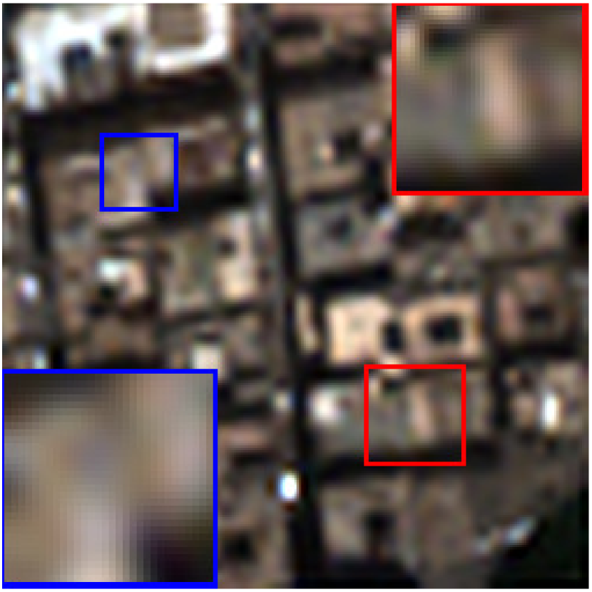
(a) EXP

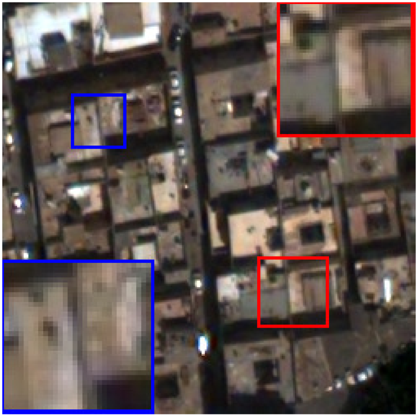
(b) GS

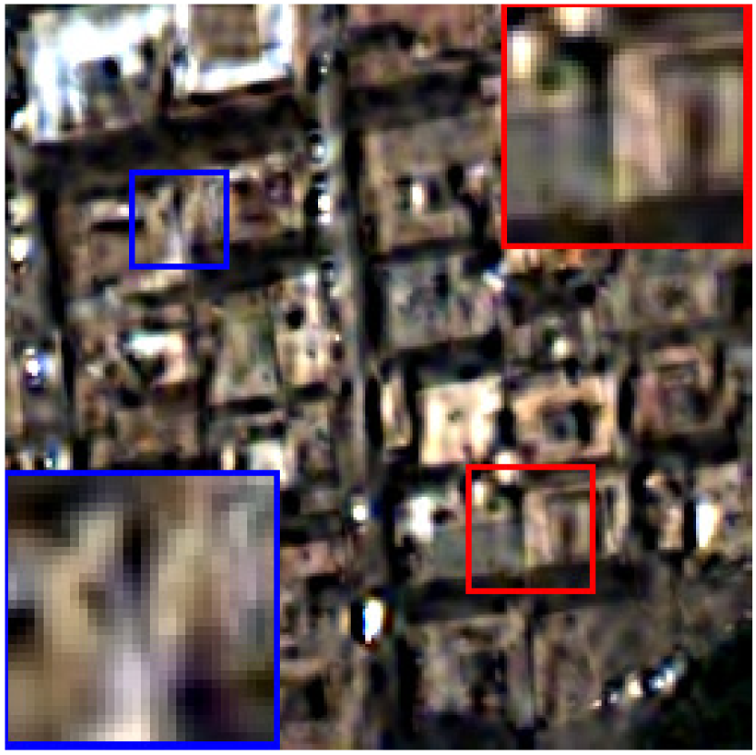
(c) BDSD

(d) BDSD-PC

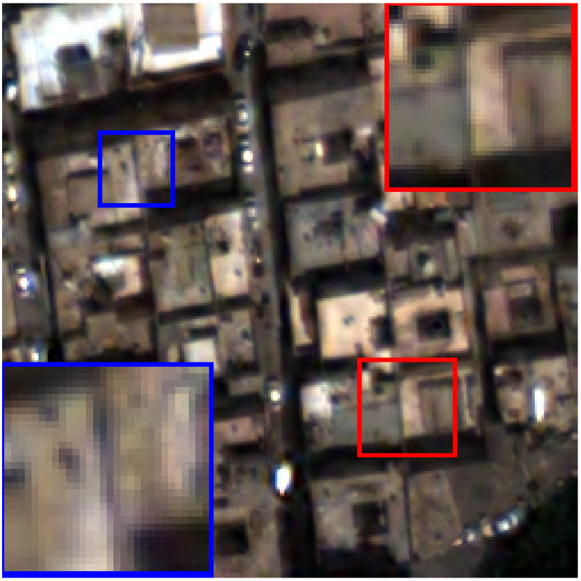
(e) PRACS

(f) AWLP

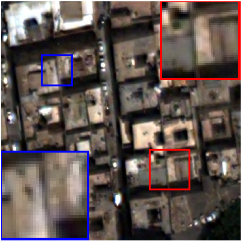
(g) GLP

(h) GLP-HPM

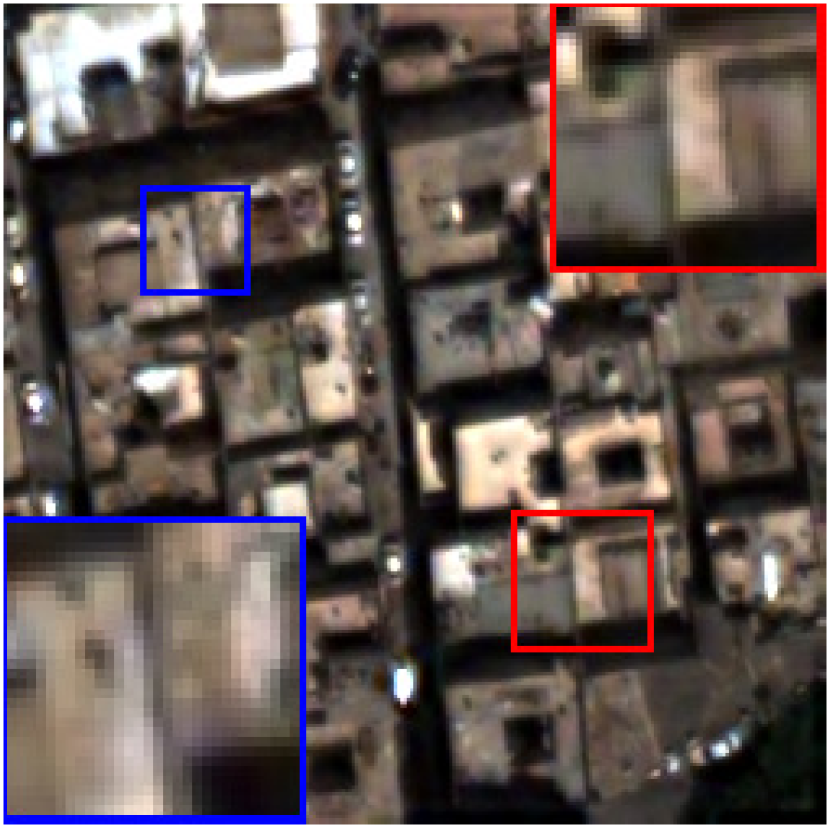
(i) MO

(j) SRD

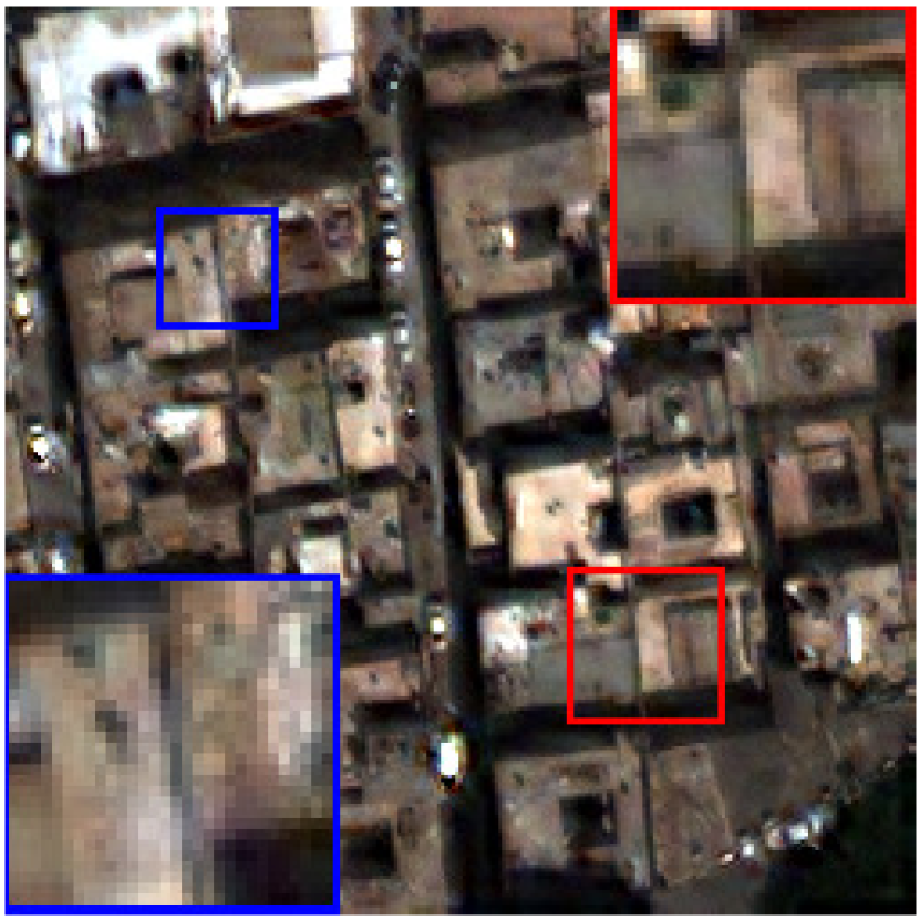
(k) PanNet

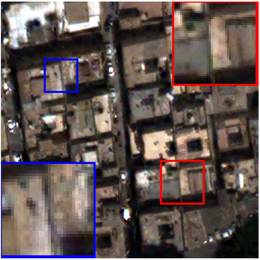
(l) Fusion-Net

(m) Our

Figure 5: Visual comparisons of the fused HRMS image for all the methods on a full resolution sample.

(a) EXP

(b) GS

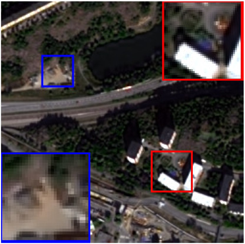
(c) BDSD

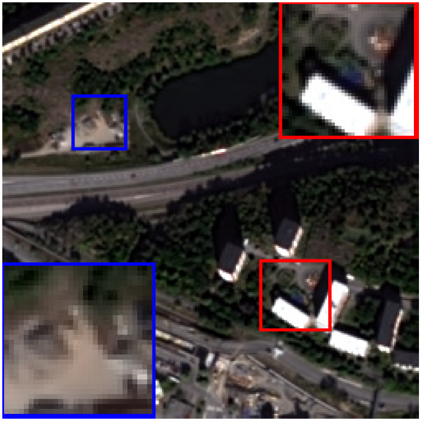
(d) BDSD-PC

(e) PRACS

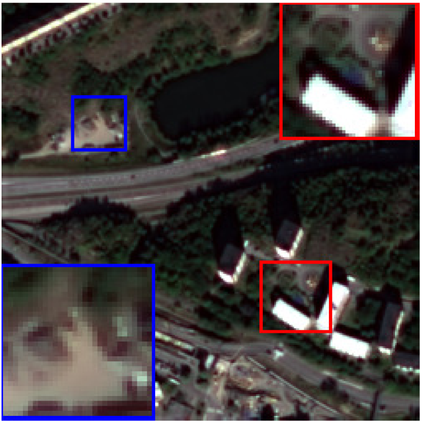
(f) AWLP

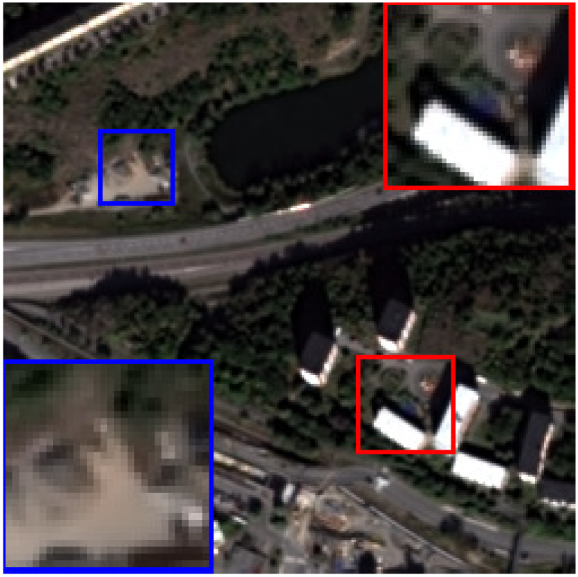
(g) GLP

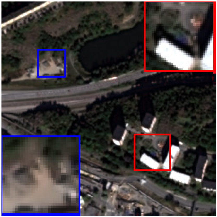
(h) GLP-HPM

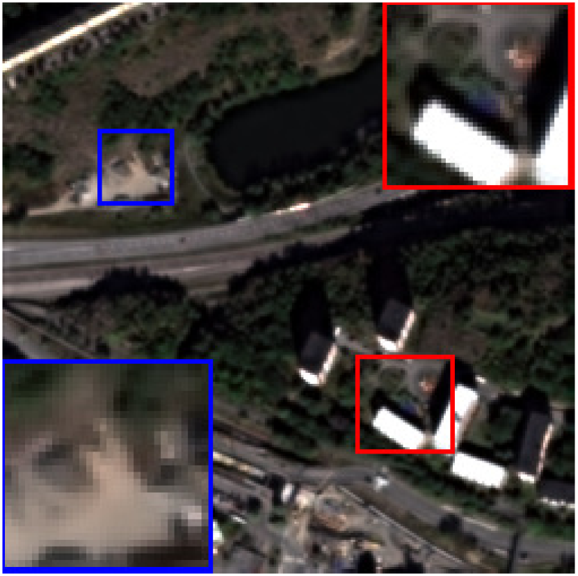
(i) MO

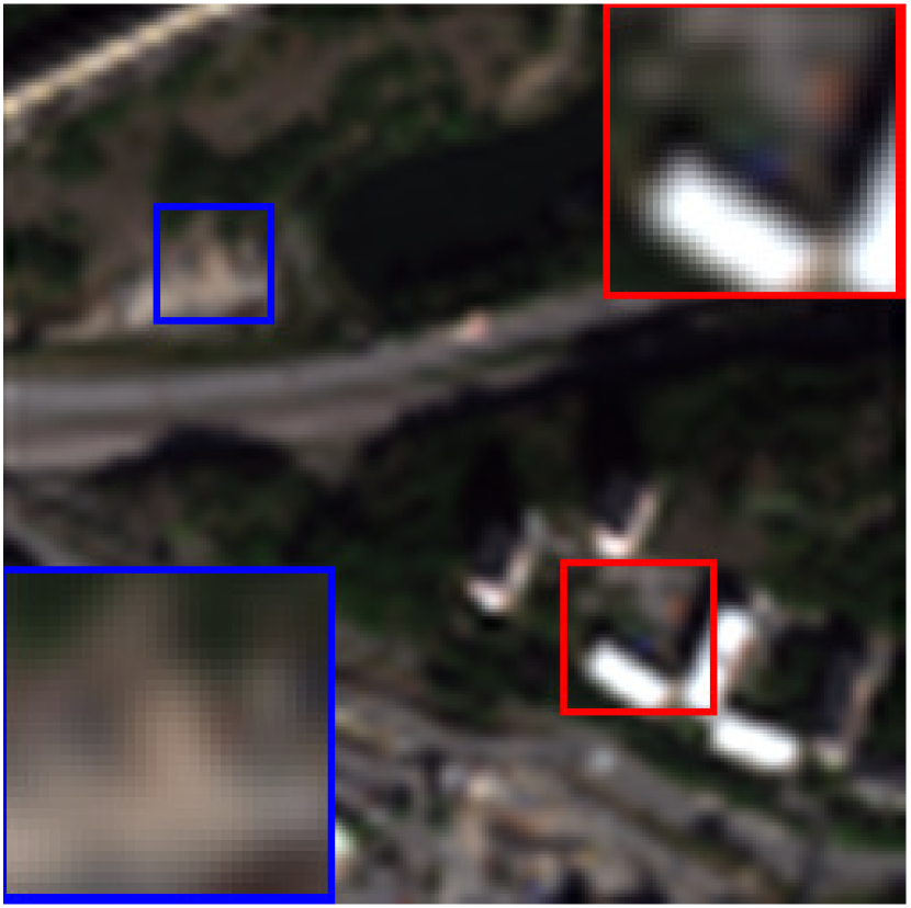
(j) SRD

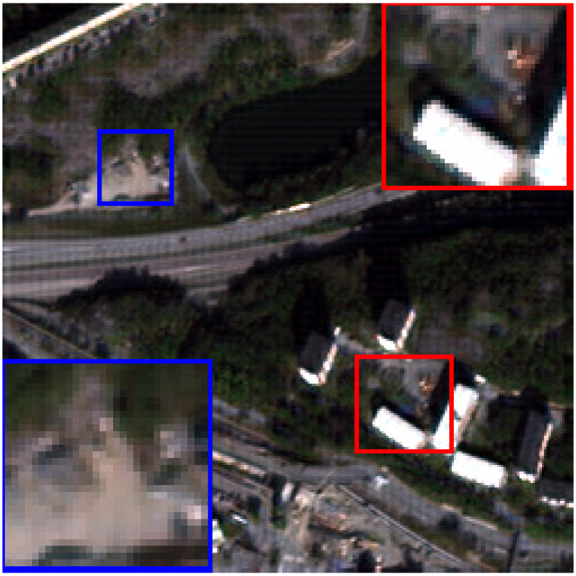
(k) PanNet

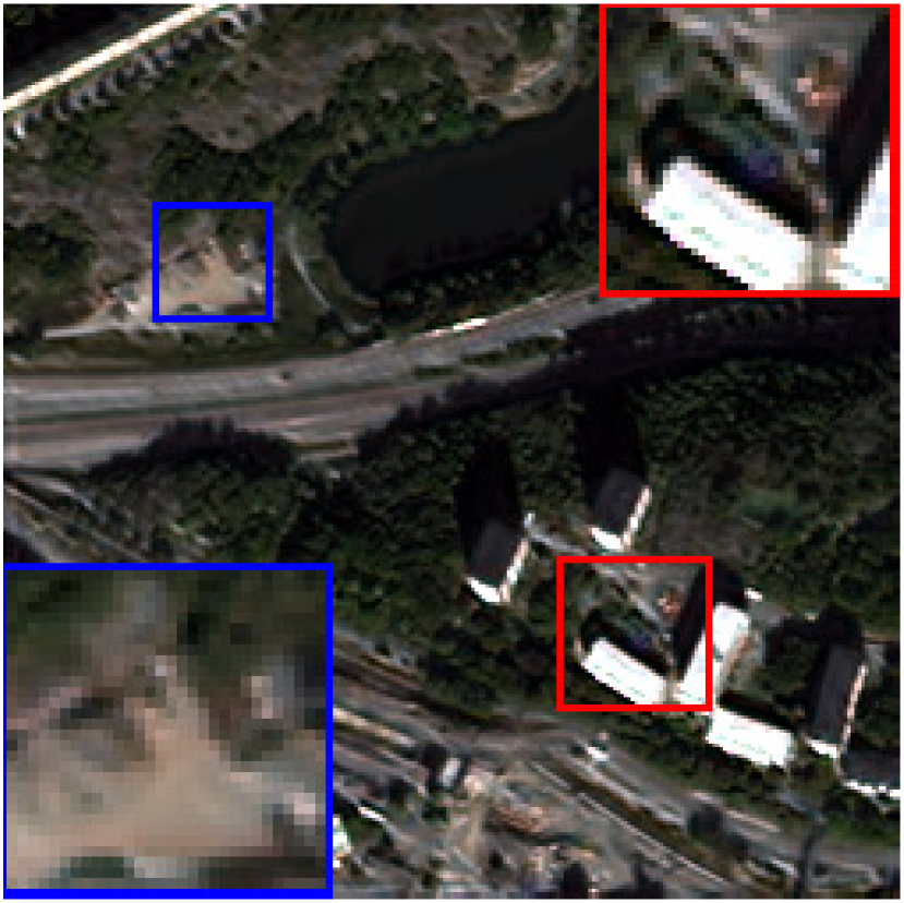
(l) Fusion-Net

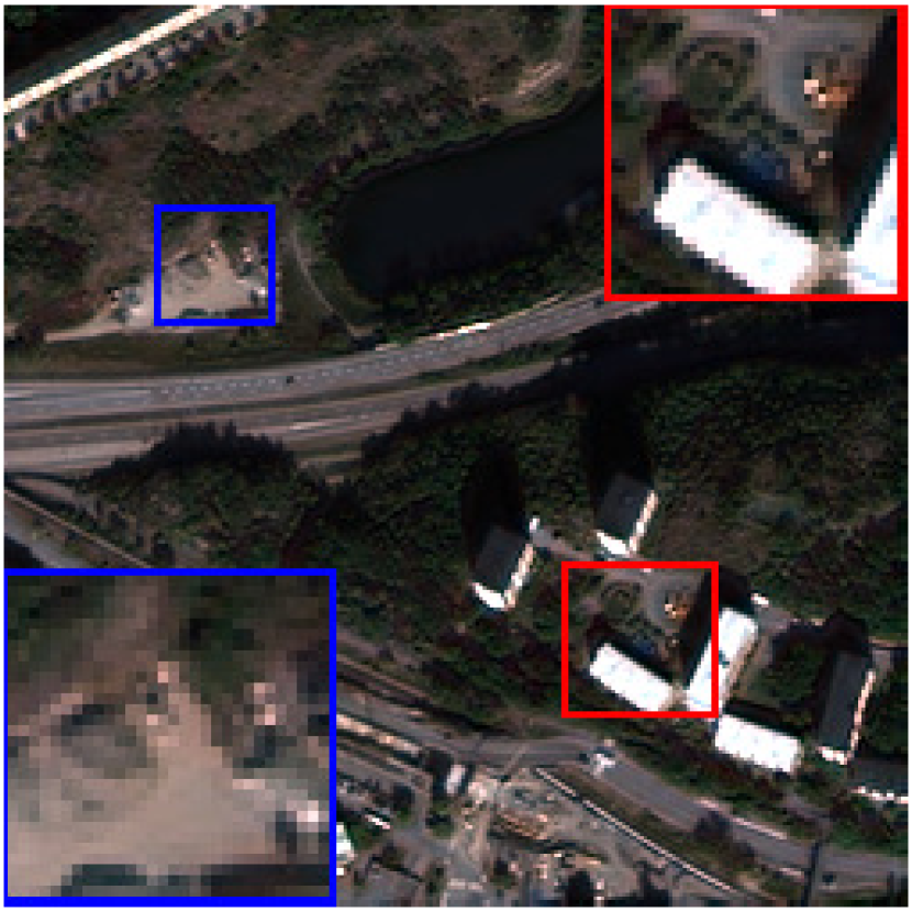
(m) Our

(n) GT

Figure 6: Visual comparisons of the fused HRMS image for all the methods on the WorldView-2 dataset.

Table 4: Average quantitative result on WorldView-2 dataset (4 samples).

Methods	Q8	SAM	ERGAS	SCC
EXP (Aiazzi et al. 2002)	0.1478$\pm$0.0993	8.4696$\pm$0.6908	8.4482$\pm$0.8586	0.7305$\pm$0.0291
GS (Laben and Brower 2000)	0.3699$\pm$0.0973	8.9007$\pm$1.1376	6.0507$\pm$0.3289	0.8982$\pm$0.0157
BDSD (Garzelli, Nencini, and Capobianco 2007)	0.3813$\pm$0.0792	8.1413$\pm$0.8517	5.6247$\pm$0.6358	0.8986$\pm$0.0154
BDSD-PC (Vivone 2019)	0.2260$\pm$0.0792	8.5559$\pm$0.8517	6.7658$\pm$0.6358	0.8727$\pm$0.0154
PRACS (Choi, Yu, and Kim 2010)	0.2344$\pm$0.1275	8.2384$\pm$0.8070	6.7702$\pm$0.5389	0.8552$\pm$0.0317
AWLP (Otazu et al. 2005)	0.4048$\pm$0.1339	8.0334$\pm$0.7286	5.8288$\pm$0.6002	0.8947$\pm$0.0318
GLP (Restaino et al. 2019)	0.3777$\pm$0.0653	7.9013$\pm$0.8200	5.5841$\pm$0.5361	0.8942$\pm$0.0216
GLP-HPM (Vivone et al. 2013)	0.3171$\pm$0.0741	8.0942$\pm$0.9487	5.8434$\pm$0.6011	0.8826$\pm$0.0220
MO (Restaino et al. 2016)	0.3381$\pm$0.1108	7.8839$\pm$0.9794	5.9212$\pm$0.5137	0.8936$\pm$0.0102
SRD (Vicinanza et al. 2014)	0.1478$\pm$0.0993	8.4696$\pm$0.6908	8.4482$\pm$0.8580	0.7305$\pm$0.0291
PanNet (Yang et al. 2017)	0.3746$\pm$0.1053	7.5776$\pm$0.6670	5.5402$\pm$0.1744	0.9144$\pm$0.0178
Fusion-Net (Deng et al. 2020)	0.3685$\pm$0.0797	8.2145$\pm$1.1321	6.1401$\pm$0.3592	0.8890$\pm$0.0187
Our	0.3885$\pm$0.1337	7.5233$\pm$0.9893	5.4103$\pm$0.1841	0.9231$\pm$0.0120
Ideal value	1	0	0	1

Parameters and Time Comparisons

In Table 5, we also report the running time, the number of parameters, and the giga floating-point operations per second (GFLOPs) of our network with some typical methods on two image sizes. From Table 5, we can find that our network has a comparable efficiency with the advanced approaches. Besides, our network has fewer parameters compared to the other two DL-based methods.

Table 5: Parameters and time comparisons.

	Image size	BDSD	AWLP	GLP	PanNet	Fusion-Net	Our
Runtime (s)	64$\times$64 (PAN) 16$\times$16$\times$8 (MS)	0.01	0.01	0.03	0.42	0.44	0.65
	256$\times$256 (PAN) 64$\times$64$\times$8 (MS)	0.02	0.08	0.12	2.63	2.31	2.79
GFLOPs	64$\times$64 (PAN) 16$\times$16$\times$8 (MS)	$4.2\times 10^{-8}$	$5.9\times 10^{-4}$	$6.5\times 10^{-5}$	0.65	0.64	0.71
	256$\times$256 (PAN) 64$\times$64$\times$8 (MS)	$4.2\times 10^{-8}$	$5.9\times 10^{-4}$	$6.5\times 10^{-5}$	10.3	10.2	11.2
$\#$ Params ($\times 10^{4}$)	-	-	-	-	7.76	7.63	7.03

Conclusion

This paper proposes a novel deep network for pansharpening using the model-based deep learning method. Specifically, we first propose a new pansharpening model based on the convolutional sparse coding technique. Then, we design a proximal gradient algorithm to solve this model, and then unfold this iterative algorithm into a network. Finally, all the learnable modules can be learned end-to-end. Since each network module corresponds to an operation of the algorithm, our network has a clear physical interpretation. This helps us to better understand how the network works. Experimental results on some benchmark datasets illustrate our network has better performance than other advanced approaches both quantitatively and qualitatively.

References

- Aiazzi et al. (2002) Aiazzi, B.; Alparone, L.; Baronti, S.; and Garzelli, A. 2002. Context-driven fusion of high spatial and spectral resolution images based on oversampled multiresolution analysis. IEEE Transactions on Geoscience and Remote Sensing, 40(10): 2300–2312.
- Beck and Teboulle (2009) Beck, A.; and Teboulle, M. 2009. A fast iterative shrinkage-thresholding algorithm for linear inverse problems. SIAM Journal on Imaging Sciences, 2(1): 183–202.
- Cao et al. (2021) Cao, X.; Fu, X.; Hong, D.; Xu, Z.; and Meng, D. 2021. PanCSC-Net: A model-driven deep unfolding method for pansharpening. IEEE Transactions on Geoscience and Remote Sensing, DOI: 10.1109/TGRS.2021.3115501.
- Carper, Lillesand, and Kiefer (1990) Carper, W.; Lillesand, T.; and Kiefer, R. 1990. The use of intensity-hue-saturation transformations for merging SPOT panchromatic and multispectral image data. Photogrammetric Engineering and Remote Sensing, 56(4): 459–467.
- Choi, Yu, and Kim (2010) Choi, J.; Yu, K.; and Kim, Y. 2010. A new adaptive component-substitution-based satellite image fusion by using partial replacement. IEEE Transactions on Geoscience and Remote Sensing, 49(1): 295–309.
- Deng, Feng, and Tai (2019) Deng, L.-J.; Feng, M.; and Tai, X.-C. 2019. The fusion of panchromatic and multispectral remote sensing images via tensor-based sparse modeling and hyper-Laplacian prior. Information Fusion, 52: 76–89.
- Deng et al. (2018) Deng, L.-J.; Vivone, G.; Guo, W.; Dalla Mura, M.; and Chanussot, J. 2018. A variational pansharpening approach based on reproducible kernel Hilbert space and heaviside function. IEEE Transactions on Image Processing, 27(9): 4330–4344.
- Deng et al. (2020) Deng, L.-J.; Vivone, G.; Jin, C.; and Chanussot, J. 2020. Detail injection-based deep convolutional neural networks for pansharpening. IEEE Transactions on Geoscience and Remote Sensing, DOI: 10.1109/TGRS.2020.3031366.
- Deng and Dragotti (2020) Deng, X.; and Dragotti, P. L. 2020. Deep convolutional neural network for multi-modal image restoration and fusion. IEEE Transactions on Pattern Analysis and Machine Intelligence, DOI: 10.1109/TPAMI.2020.2984244.
- Dong et al. (2021) Dong, W.; Zhou, C.; Wu, F.; Wu, J.; Shi, G.; and Li, X. 2021. Model-guided deep hyperspectral image super-resolution. IEEE Transactions on Image Processing, DOI: 10.1109/TIP.2021.3078058.
- Fang et al. (2013a) Fang, F.; Li, F.; Shen, C.; and Zhang, G. 2013a. A variational approach for pan-sharpening. IEEE Transactions on Image Processing, 22(7): 2822–2834.
- Fang et al. (2013b) Fang, F.; Li, F.; Zhang, G.; and Shen, C. 2013b. A variational method for multisource remote-sensing image fusion. International Journal of Remote Sensing, 34(7): 2470–2486.
- Fu et al. (2019) Fu, X.; Lin, Z.; Huang, Y.; and Ding, X. 2019. A variational pan-sharpening with local gradient constraints. In Proceedings of the IEEE/CVF Conference on Computer Vision and Pattern Recognition, 10265–10274.
- Fu et al. (2020) Fu, X.; Wang, W.; Huang, Y.; Ding, X.; and Paisley, J. 2020. Deep multiscale detail networks for multiband spectral image sharpening. IEEE Transactions on Neural Networks and Learning Systems, 32(5): 2090–2104.
- Garzelli, Nencini, and Capobianco (2007) Garzelli, A.; Nencini, F.; and Capobianco, L. 2007. Optimal MMSE pan sharpening of very high resolution multispectral images. IEEE Transactions on Geoscience and Remote Sensing, 46(1): 228–236.
- He et al. (2016) He, K.; Zhang, X.; Ren, S.; and Sun, J. 2016. Deep residual learning for image recognition. In Proceedings of the IEEE Conference on Computer Vision and Pattern Recognition, 770–778.
- He et al. (2019) He, L.; Rao, Y.; Li, J.; Chanussot, J.; Plaza, A.; Zhu, J.; and Li, B. 2019. Pansharpening via detail injection based convolutional neural networks. IEEE Journal of Selected Topics in Applied Earth Observations and Remote Sensing, 12(4): 1188–1204.
- Huang et al. (2015) Huang, W.; Xiao, L.; Wei, Z.; Liu, H.; and Tang, S. 2015. A new pan-sharpening method with deep neural networks. IEEE Geoscience and Remote Sensing Letters, 12(5): 1037–1041.
- Laben and Brower (2000) Laben, C. A.; and Brower, B. V. 2000. Process for enhancing the spatial resolution of multispectral imagery using pan-sharpening. US Patent 6,011,875.
- Li et al. (2021) Li, M.; Cao, X.; Zhao, Q.; Zhang, L.; and Meng, D. 2021. Online rain/snow removal from surveillance videos. IEEE Transactions on Image Processing, 30: 2029–2044.
- Li and Yang (2010) Li, S.; and Yang, B. 2010. A new pan-sharpening method using a compressed sensing technique. IEEE Transactions on Geoscience and Remote Sensing, 49(2): 738–746.
- Liu (2000) Liu, J. 2000. Smoothing filter-based intensity modulation: A spectral preserve image fusion technique for improving spatial details. International Journal of Remote Sensing, 21(18): 3461–3472.
- Masi et al. (2016) Masi, G.; Cozzolino, D.; Verdoliva, L.; and Scarpa, G. 2016. Pansharpening by convolutional neural networks. Remote Sensing, 8(7): 594.
- Otazu et al. (2005) Otazu, X.; González-Audícana, M.; Fors, O.; and Núñez, J. 2005. Introduction of sensor spectral response into image fusion methods. Application to wavelet-based methods. IEEE Transactions on Geoscience and Remote Sensing, 43(10): 2376–2385.
- Restaino et al. (2019) Restaino, R.; Vivone, G.; Addesso, P.; and Chanussot, J. 2019. A pansharpening approach based on multiple linear regression estimation of injection coefficients. IEEE Geoscience and Remote Sensing Letters, 17(1): 102–106.
- Restaino et al. (2016) Restaino, R.; Vivone, G.; Dalla Mura, M.; and Chanussot, J. 2016. Fusion of multispectral and panchromatic images based on morphological operators. IEEE Transactions on Image Processing, 25(6): 2882–2895.
- Shah, Younan, and King (2008) Shah, V. P.; Younan, N. H.; and King, R. L. 2008. An efficient pan-sharpening method via a combined adaptive PCA approach and contourlets. IEEE Transactions on Geoscience and Remote Sensing, 46(5): 1323–1335.
- Tian et al. (2021) Tian, X.; Chen, Y.; Yang, C.; and Ma, J. 2021. Variational pansharpening by exploiting cartoon-texture similarities. IEEE Transactions on Geoscience and Remote Sensing, DOI: 10.1109/TGRS.2020.3048257.
- Vicinanza et al. (2014) Vicinanza, M. R.; Restaino, R.; Vivone, G.; Dalla Mura, M.; and Chanussot, J. 2014. A pansharpening method based on the sparse representation of injected details. IEEE Geoscience and Remote Sensing Letters, 12(1): 180–184.
- Vivone (2019) Vivone, G. 2019. Robust band-dependent spatial-detail approaches for panchromatic sharpening. IEEE Transactions on Geoscience and Remote Sensing, 57(9): 6421–6433.
- Vivone et al. (2014) Vivone, G.; Alparone, L.; Chanussot, J.; Dalla Mura, M.; Garzelli, A.; Licciardi, G. A.; Restaino, R.; and Wald, L. 2014. A critical comparison among pansharpening algorithms. IEEE Transactions on Geoscience and Remote Sensing, 53(5): 2565–2586.
- Vivone, Marano, and Chanussot (2020) Vivone, G.; Marano, S.; and Chanussot, J. 2020. Pansharpening: context-based generalized Laplacian pyramids by robust regression. IEEE Transactions on Geoscience and Remote Sensing, 58(9): 6152–6167.
- Vivone, Restaino, and Chanussot (2018) Vivone, G.; Restaino, R.; and Chanussot, J. 2018. Full scale regression-based injection coefficients for panchromatic sharpening. IEEE Transactions on Image Processing, 27(7): 3418–3431.
- Vivone et al. (2013) Vivone, G.; Restaino, R.; Dalla Mura, M.; Licciardi, G.; and Chanussot, J. 2013. Contrast and error-based fusion schemes for multispectral image pansharpening. IEEE Geoscience and Remote Sensing Letters, 11(5): 930–934.
- Wald, Ranchin, and Mangolini (1997) Wald, L.; Ranchin, T.; and Mangolini, M. 1997. Fusion of satellite images of different spatial resolutions: Assessing the quality of resulting images. Photogrammetric Engineering and Remote Sensing, 63(6): 691–699.
- Wang et al. (2018) Wang, T.; Fang, F.; Li, F.; and Zhang, G. 2018. High-quality Bayesian pansharpening. IEEE Transactions on Image Processing, 28(1): 227–239.
- Xie et al. (2020a) Xie, Q.; Zhou, M.; Zhao, Q.; Xu, Z.; and Meng, D. 2020a. MHF-net: An interpretable deep network for multispectral and hyperspectral image fusion. IEEE Transactions on Pattern Analysis and Machine Intelligence, DOI: 10.1109/TPAMI.2020.3015691.
- Xie et al. (2020b) Xie, W.; Cui, Y.; Li, Y.; Lei, J.; Du, Q.; and Li, J. 2020b. HPGAN: Hyperspectral pansharpening using 3-D generative adversarial networks. IEEE Transactions on Geoscience and Remote Sensing, 59(1): 463–477.
- Yang et al. (2017) Yang, J.; Fu, X.; Hu, Y.; Huang, Y.; Ding, X.; and Paisley, J. 2017. PanNet: A deep network architecture for pan-sharpening. In Proceedings of the IEEE International Conference on Computer Vision, 5449–5457.
- Yang et al. (2021) Yang, Y.; Tu, W.; Huang, S.; Lu, H.; Wan, W.; and Gan, L. 2021. Dual-stream convolutional neural network with residual information enhancement for pansharpening. IEEE Transactions on Geoscience and Remote Sensing, DOI: 10.1109/TGRS.2021.3098752.
- Yin (2021) Yin, H. 2021. PSCSC-Net: A deep coupled convolutional sparse coding network for pansharpening. IEEE Transactions on Geoscience and Remote Sensing, DOI: 10.1109/TGRS.2021.3088313.
- Yuan et al. (2018) Yuan, Q.; Wei, Y.; Meng, X.; Shen, H.; and Zhang, L. 2018. A multiscale and multidepth convolutional neural network for remote sensing imagery pan-sharpening. IEEE Journal of Selected Topics in Applied Earth Observations and Remote Sensing, 11(3): 978–989.
- Zhang and Ma (2021) Zhang, H.; and Ma, J. 2021. GTP-PNet: A residual learning network based on gradient transformation prior for pansharpening. ISPRS Journal of Photogrammetry and Remote Sensing, 172: 223–239.
- Zhou, Liu, and Wang (2021) Zhou, H.; Liu, Q.; and Wang, Y. 2021. Pgman: An unsupervised generative multiadversarial network for pansharpening. IEEE Journal of Selected Topics in Applied Earth Observations and Remote Sensing, 14: 6316–6327.