HIP-2022-2/TH

NORDITA 2022-009

Combining thermal resummation and gauge invariance for electroweak phase transition

Philipp Schicho^a,, Tuomas V. I. Tenkanen^b,c,d, and Graham White^e,

^aDepartment of Physics and Helsinki Institute of Physics,
P.O. Box 64, FI-00014 University of Helsinki, Finland

${}^{\mbox{\scriptsize b}}$Nordita, KTH Royal Institute of Technology and Stockholm University,
Roslagstullsbacken 23, SE-106 91 Stockholm, Sweden

${}^{\mbox{\scriptsize c}}$Tsung-Dao Lee Institute & School of Physics and Astronomy,
Shanghai Jiao Tong University, Shanghai 200240, China

${}^{\mbox{\scriptsize d}}$Shanghai Key Laboratory for Particle Physics and Cosmology, Key Laboratory for Particle Astrophysics and Cosmology (MOE), Shanghai Jiao Tong University,
Shanghai 200240, China

${}^{\mbox{\scriptsize e}}$Kavli IPMU (WPI), UTIAS, The University of Tokyo, Kashiwa, Chiba 277-8583, Japan

Abstract

For computing thermodynamics of the electroweak phase transition, we discuss a minimal approach that reconciles both gauge invariance and thermal resummation. Such a minimal setup consists of a two-loop dimensional reduction to three-dimensional effective theory, a one-loop computation of the effective potential and its expansion around the leading-order minima within the effective theory. This approach is tractable and provides formulae for resummation that are arguably no more complicated than those that appear in standard techniques ubiquitous in the literature. In particular, we implement renormalisation group improvement related to the hard thermal scale. Despite its generic nature, we present this approach for the complex singlet extension of the Standard Model which has interesting prospects for high energy collider phenomenology and dark matter predictions. The presented expressions can be used in future studies of phase transition thermodynamics and gravitational wave production.

1 Introduction

Understanding the thermal history of electroweak symmetry breaking is one of the central endeavours of next generation experiments, with both next generation colliders [1, 2, 3] and gravitational wave detectors [4] potentially giving definitive answers. Furthermore, if electroweak symmetry breaking occurs via a strong first-order phase transition, it could answer one of the central issues of cosmology – why is there more matter than anti-matter in the present day universe [5, 6]. Since the Standard Model (SM) of particle physics predicts a smooth crossover transition [7, 8, 9, 10, 11], modifying this expectation necessitates new beyond the Standard Model (BSM) states at the electroweak scale [12, 13, 14, 15, 16, 17, 18, 19, 20, 21, 22, 23, 24, 25, 26, 27, 28, 29, 30, 31, 32, 33, 34, 35, 36, 37, 38, 39, 40, 41, 42, 43, 44, 45, 46, 47, 48, 49]. In the presence of a global symmetry, among such new states could in fact be a dark matter candidate [50, 51, 52, 28, 39], giving a minimal unified explanation for the origin of matter.

Describing the electroweak phase transition (EWPT) perturbatively is a theoretical challenge. In non-Abelian gauge theories at finite temperature, perturbation theory fails completely at high enough orders [53]. Even at lower orders, the effective expansion parameter can be large despite a weakly coupled zero-temperature theory. Physically, this is a consequence of enhancement of light bosonic modes at the infrared (IR), and for a perturbative description to converge requires thermal resummations. The thermal plasma exhibits a class of mass hierarchies at high temperature, and in perturbation theory this can be described by integrating out contributions of the heavy thermal scale to parameters of an effective theory at lower scales [54]. This idea of effective descriptions is systematised by high-temperature dimensional reduction [55, 56] to three-dimensional effective field theory (3d EFT) [57, 58]. Dimensional reduction allows to by-pass problems of perturbation theory at the infrared using non-perturbative lattice simulations of the 3d EFT [59, 7]. Due to the excessive cost and technical effort of such simulations, the virtue of perturbation theory within the 3d EFT [60] is to guide thermodynamic investigations.

Past decade EWPT analyses most often focused on minimising the thermal effective potential that adopts the resummation of “the most dangerous daisy diagrams”. At leading order, this is achieved by resumming one-loop thermal corrections to masses of zero Matsubara modes and subsequently computing the one-loop effective potential for the resummed zero modes. The 3d EFT picture translates this to a dimensional reduction at leading order (one-loop in effective masses, tree-level in couplings) and a computation of the one-loop effective potential within the EFT. On the other hand, this description fails to include several important two-loop contributions [54, 61]. Without these two-loop contributions, leading renormalisation group improvement is incomplete [54, 60, 62]. Such an improvement cancels the renormalisation scale between the running of leading-order contributions and explicit logarithmic terms at next-to-leading order (NLO). Indeed, due to the slower convergence of perturbation theory at high temperature, this cancellation requires a two-loop level computation as a subset of leading logarithms only appears at this loop level. Recent work [44, 63, 64, 62] has stressed the numerical importance of a consistent perturbative computation to account for these effects in BSM scenarios of the electroweak phase transition.

Conventional methods for studying the electroweak phase transition in BSM theories suffer from an undesired gauge dependence [65] during a direct numerical minimisation of the daisy-resummed thermal effective potential. One established method for removing this gauge dependence is to perform an “$\hbar$-expansion”. There, the effective potential is expanded around its leading-order minima [66, 65]. In this expansion, the Nielsen identities [67, 68] guarantee gauge independence.

In the PRM scheme [65], gauge invariance comes at the cost of neglecting important resummations of infrared enhanced diagrams when calculated at $\mathcal{O}(\hbar)$. The article at hand resolves this technical issue and describes an improved approach, where (A) thermal resummations are handled by the dimensionally reduced 3d EFT with (B) an $\hbar$-expansion applied within the EFT. Gauge invariance is ensured at each step individually. This approach was originally devised in [66] and recently applied in [69, 63, 62] (also cf. [70]). However, here we present important updates: for radiatively generated transitions, we resum one-loop contributions from heavy fields together with tree-level terms to the leading order potential [61, 71, 72, 73]. Hence, the barrier required for a first-order phase transition is already present at leading order (LO) in perturbation theory. This can furthermore help to avoid a spurious infrared divergence encountered at higher orders [66, 69]. In particular, we advocate a minimal setup with NLO dimensional reduction to 3d EFT (two-loop in masses, one-loop in couplings), and a one-loop computation of the effective potential within the EFT. When determining the critical temperature ($T_{\rm c}$) and other thermodynamic quantities of interest, we resort to a technique described in [65, 69] rather than expanding $T_{\rm c}$ explicitly in $\hbar$ as in [66].

All ingredients of our approach have appeared individually in earlier literature [60, 66, 58, 57, 65, 71, 72, 73]. Here, we uniquely apply them together for the first time with a BSM application. An another similar combination of thermal resummation and gauge invariance was recently developed [71]. This reference uses a direct computation with consistent power counting to ensure gauge invariance instead of the 3d EFT approach. The power of the 3d EFT approach has been further demonstrated in a novel technique for thermal bubble nucleation [72] which was applied in [73] (cf. [74, 75] and related [76, 77]). Principally, the approach suggested in the article at hand can be embedded in a more generic framework [72].

The proposed approach applies to a wide range of BSM theories of the electroweak phase transition. One such theory is the complex-singlet extension of the Standard Model (cxSM) [16] for which we present our prescription. The model contains two new scalar states, one that could form a stable dark matter candidate and one that participates dynamically in the phase transition. This renders the model an appealing minimal BSM candidate for both dark matter and a potentially strong electroweak phase transition. Recent literature has debated of how to organise the perturbative computation of cxSM thermodynamics. Ref. [28] includes leading daisy resummations, but lacks gauge invariance, while ref. [39] maintains gauge invariance at the cost of resummation (also cf. [79] and a more recent investigation [80]). Similar confusion can in principle arise in any BSM model. Our computation combines the benefits of both previous studies and also improves them by removing their aforementioned shortcomings. Consistent with [63, 62], we find significant error arising from omitting two-loop corrections to thermal masses. The takeaway message of this article is that such corrections should not be omitted. We furthermore demonstrate how to implement them in a gauge-invariant manner.

The structure of this article is as follows. Section 2 summarises our approach, introduces the model and its 3d EFT at high temperature, and describes the computation of thermodynamics. In addition, we review the perturbative expansion for the effective potential. In section 3 we numerically demonstrate our approach at a representative benchmark point. Section 4 summarises our findings and discusses their application for potential future parameter space scans. Appendix A collects technical details and explicates formulae of our analysis. Finally, appendix Epilogue discusses renormalisation group improvement and an epilogue therein exemplifies the importance of including thermal masses at two-loop order, in a toy model of the SM with an artificially light Higgs.

2 Thermodynamics: resummation and gauge invariance

Figure 1: Schematic illustration of a perturbative 3d EFT computation of thermodynamics. This article advocates a novel prescription for combining $(1)\to(2)\to(3)$ (cf. sec. 2). This specific implementation aligns with the generic steps $(d)\to(e)\to(f)$ in fig. 2 in [81].

This technical section details our computation. In fig. 1, we schematically outline the computation of thermodynamics, adapted from [81]. The novel prescription suggested in this article combines

• Dimensional reduction to 3d EFT at NLO [58] which determines thermal masses up-to two-loo level.

• Computing the effective potential within the 3d EFT [60] at one-loop level and in $\hbar$-expansion [66]. For a radiative barrier, heavy field contributions at one-loop level are resummed to the potential at LO [72, 73, 82, 83].

• Determining critical temperatures numerically from a condition that the value of the effective potential at different phases is degenerate [65] as well as determining gauge-invariant condensates and latent heat [59, 69].

For (1), it is crucial that thermal resummation by dimensional reduction is performed at NLO, instead of LO. The NLO corrections are sizable, which is already indicated by a large RG scale dependence of the LO computation [63, 62]. Typical computations of the thermal effective potential at one-loop level resum also masses at one-loop. Such resummation matches the accuracy of the LO dimensional reduction, and is hence insufficient to eliminate large RG scale dependence.

In (2), we have chosen practicality over full RG improvement. The computation of the 3d effective potential is straightforward at one-loop, as one only needs background field dependent mass eigenvalues. However, RG improvement related to the 3d EFT RG scale can only be eliminated at two-loop order [60]. Naturally, such a computation is more challenging (cf. [66, 69, 63, 81]). However, we demonstrate that in practice the dependence on an uneliminated 3d RG scale is less severe as the aforementioned dependence on 4d RG scale – a trend demonstrated already in [63].

In (3), our numerical implementation follows [65, 69] and differs from the strategy in [66, 63]. There, the critical temperature itself is expanded in $\hbar$ and solved order-by-order.

The remainder of this section details our conventions for the complex-singlet extension of the Standard Model (cxSM), the structure of the corresponding 3d EFT, a review of the perturbative expansion, the thermal effective potential within the EFT and a gauge-invariant computation of the thermodynamic quantities of interest. Several formulae are collected in appendix A, for a reader to replicate our analysis. While our discussion and concrete expressions focus on the cxSM, we present the underlying ideas generically, for them to be applied in other BSM theories. In particular, we advocate that our prescription could be implemented in software for analysing the electroweak phase transition, such as CosmoTransitions [84], BSMPT [85, 86], and PhaseTracer [87].

2.1 A complex-singlet extended Standard Model

We use the model of ref. [39] with the Standard Model augmented by a complex singlet scalar $S$, abbreviated as the cxSM. The scalar sector of the full 4d Lagrangian in Euclidean space reads

$$\mathcal{L}^{\text{4d}}_{\text{scalar}} =(D_{\mu}\phi)^{\dagger}(D_{\mu}\phi)+\mu_{h}^{2}\phi^{\dagger}\phi+\lambda_{h}(\phi^{\dagger}\phi)^{2}$$

$$+\frac{1}{2}(\partial_{\mu}S^{*})(\partial_{\mu}S)+\frac{1}{2}b_{2}S^{*}S+\frac{1}{4}d_{2}(S^{*}S)^{2}$$

$$+\frac{1}{2}\delta_{2}S^{*}S\phi^{\dagger}\phi+a_{1}S+a^{*}_{1}S^{*}+\frac{1}{4}\Big{(}b_{1}SS+b^{*}_{1}S^{*}S^{*}\Big{)}\;.$$ (2.1)

The scalar fields are parametrised as

$$\phi =\begin{pmatrix}G^{+}\\ \frac{1}{\sqrt{2}}(v_{0}+h+iz)\end{pmatrix}\;,\quad\quad S=\frac{1}{\sqrt{2}}(v_{S_{0}}+s+iA)\;,$$ (2.2)

where $v_{0}$ and $v_{S_{0}}$ are zero-temperature real vacuum-expectations-values (VEV) and $G^{-}=(G^{+})^{\dagger}$. After electroweak symmetry breaking, this model has three scalar eigenstates: two CP-even eigenstates resulting from mixing $h$ and $s$, and one CP-odd state, $A$. All complex phases that can mix $s$ and $A$ are assumed to be zero. The SM-like Higgs boson is one of the CP-even fields, and $A$ is the dark matter candidate. The fields $G^{\pm}$ and $z$ are the usual Nambu-Goldstone bosons as in the SM. A tree-level analysis of relations between the Lagrangian parameters above (in $\overline{\text{MS}}$ -scheme) and the parameters of the mass eigenstate basis can be found in [39] and we merely collect the relevant relations in appendix A.1. We follow conventions of [88, 81] for the SM field content. The one-loop renormalisation group equations for the $\overline{\text{MS}}$ -parameters are collected in appendix A.2. Below, we compute selected thermodynamic properties in terms of $\overline{\text{MS}}$ -parameters of the Lagrangian. Only when turning to numerics, we express these parameters in terms of physical quantities.

2.2 High temperature 3d EFT

At sufficiently high temperatures, the equilibrium thermodynamics of a weakly interacting quantum field theory (with weak coupling constant, $g$) in the Matsubara formalism can be described by a dimensionally reduced effective theory (cf. [57, 58]). Therein the three-dimensional zero Matsubara modes at the soft/light scale (with masses $\sim gT$) are screened by the hard/heavy non-zero Matsubara modes (with masses $\sim\pi T$). Technically, we shall work at the ultrasoft scale ($g^{2}T$) EFT. This means that in addition to the hard non-zero Matsubara modes, also the soft temporal scalar fields have been integrated out and only the ultrasoft fields remain. These include fields driving the transition (doublet and singlet) and spatial gauge fields.

The dimensionally reduced high-temperature effective theory for the cxSM is parametrically of the same form as its 4d parent theory in eq. (2.1). We do not restate the scalar Lagrangian for the doublet and singlet fields that defines the 3d EFT, but merely label its parameters with the subscript 3. Quartic couplings in the 3d EFT have dimension of mass ($T$), and fields have dimension $T^{\frac{1}{2}}$. We present an effective theory valid at next-to-leading order in dimensional reduction, namely one-loop in couplings and fields and two-loop for masses (except one-loop for parameter $b_{1,3}$). This corresponds to the formal power counting

$$\lambda_{h},d_{2},\delta_{2}\sim g^{2}\;,\qquad\mu^{2}_{h},b_{2},b_{1}\sim(gT)^{2}\;,$$ (2.3)

that is accurate to $\mathcal{O}(g^{4})$. In the absence of cubic couplings, the tadpole parameter ($a_{1,3}$) does not receive any loop corrections. Accuracy higher than $\mathcal{O}(g^{4})$, namely $\mathcal{O}(g^{6})$, would require additional higher dimensional operators [58].

The derivation of the dimensional reduction matching relations for generic models – i.e. presenting 3d parameters as a function of temperature and parameters of parent theory – has been demonstrated for example in [58] in particular for the SM and for a real singlet in a recent tutorial [81] (cf. also [89, 64]). By extending this computation to the case of a complex singlet, we derive the matching relations presented in appendix A.4. We have explicitly verified their gauge invariance: matching relations at $\mathcal{O}(g^{4})$ are independent of the gauge fixing choice of the parent 4d theory. We emphasise, that in general dimensional reduction at NLO (and at LO) is a gauge-invariant by construction; see [90, 60, 58, 63, 81, 73]. For the past two decades, the popularity of the 3d EFT approach for the EWPT phase transition thermodynamics has been superseded by that of lower order computations. One presumable bottleneck denying more applications, is the inability to perform dimensional reduction at NLO. In this regard, we advocate upcoming software [91] that helps to avoid biting the bullet and automates such computations for user-defined models.

To capture non-perturbative IR effects related to the ultrasoft scale, lattice Monte Carlo simulations of the 3d EFT [60, 7, 89] are required. For the cxSM, these simulations are out of scope of this work. The remainder of the article, concentrates on the perturbative computation of thermodynamics. While inferior, and crucially lacking even a qualitatively correct description for certain cases, these perturbative studies are computationally much less expensive and can be used as a first approximation and valuable guidance for future simulations. Nonetheless, the 3d EFT mapping presented in appendix A.4 is one of the key ingredients for such simulations. In addition, one needs lattice-continuum relations (cf. [92, 93]), simulation code including proper Monte Carlo update algorithms (for a recent application, see [89] and references therein), and a computation cluster.

2.3 Thermal effective potential in perturbation theory

The central quantity for equilibrium thermodynamics is the free energy of the system, or the effective potential for homogeneous field configurations. We begin by recalling the perturbative expansion of this quantity, along the lines of [62] (also cf. [60], and further e.g. [94, 95, 96, 97, 70] in the context of the QCD and electroweak pressure).

Perturbative expansion

At zero temperature, the effective potential admits a formal expansion in $g^{2}$, resulting in

$$V^{T=0}_{\text{eff}}=\underbrace{A_{2}g^{2}(\mu)}_{\text{tree-level}}+\underbrace{A_{4}[\ln\mu]g^{4}}_{\text{1-loop}}+\underbrace{A_{6}g^{6}}_{\text{2-loop}}+\ldots\;.$$ (2.4)

We indicate the loop order at which each contribution arises. In this case, the loop expansion aligns with the expansion in $g^{2}$. Furthermore, we emphasised the leading dependence on the renormalisation scale $\mu$ (in dimensional regularisation): at tree-level an explicit dependence on this scale does not occur, but couplings are implicit functions of $\mu$. This scale dependence, or running, is governed by renormalisation group equations, or beta functions $\mu\frac{{\rm d}}{{\rm d}\mu}g^{2}\equiv\beta(g^{2})$. At one-loop order, these beta functions match the coefficients of the logarithmic terms in $A_{4}\equiv A_{4}[\ln\mu]$ at one-loop level such that $\mu$-dependence cancels, viz.

$$\mu\frac{{\rm d}}{{\rm d}\mu}V^{T=0}_{{\mbox{\tiny\rm{eff}}}}\stackrel{{\scriptstyle{\mbox{\tiny\rm{1-loop}}}}}{{=}}\mathcal{O}(g^{6})\;.$$ (2.5)

This is the renormalisation group (RG) improvement at one-loop level. It manifests when couplings are solved from their one-loop beta functions. At higher loop levels, similar cancellations occur when including higher-order beta functions and logarithmic terms. The key feature of the perturbative expansion at zero temperature is that the full $\mathcal{O}(g^{4})$ accuracy, with corresponding RG improvement, can be achieved by a mere one-loop computation. Furthermore, an error made by truncating at one-loop is parametrically of $\mathcal{O}(g^{6})$.

The situation is more challenging in high-temperature perturbation theory. Due to the enhancement of IR bosonic modes and subsequent resummations in perturbation theory, the formal expansion of the effective potential reads

$$V^{\text{thermal}}_{\text{eff}}=\underbrace{a_{2}g^{2}}_{\begin{subarray}{c}\text{tree-level}\\ \text{1-loop}\end{subarray}}+\underbrace{a_{3}g^{3}}_{\text{1-loop}}+\underbrace{a_{4}g^{4}}_{\begin{subarray}{c}\text{1-loop}\\ \text{2-loop}\end{subarray}}+\underbrace{a_{5}g^{5}}_{\text{3-loop}}+\ldots\;.$$ (2.6)

The potential is parametrically slower convergent than at zero temperature as an expansion is in $g$ instead of $g^{2}$. Hence, to achieve the same accuracy as at zero-$T$ requires the computation of higher loop levels. In more detail

• $g^{2}$-terms arise both at tree-level and from one-loop thermal corrections to masses.

• $g^{3}$-terms arise solely at one-loop level in the 3d EFT for soft contributions.

• $g^{4}$-terms comprise of:

  • one-loop hard contributions in quartic terms,

  • one-loop field renormalisation contributions,

  • two-loop hard contributions to masses and one-loop mass corrections in the high temperature expansion,

  • two-loop soft contributions within the 3d EFT.

• $g^{5}$-terms appear at three-loop level in 3d EFT [98].

The NLO one-loop term matches usual “daisy resummation” when only the mass parameters are resummed by hard thermal corrections. Practically, in the 3d EFT approach also higher order resummations are automatically included since also couplings are resummed and masses include two-loop corrections. Truncated terms at $\mathcal{O}(g^{6})$ include two- and three-loop hard contributions, contributions to higher dimensional operators in the 3d EFT, and four-loop soft contributions within 3d EFT.

Considering the above breakdown, typical one-loop approximations of the thermal effective potential are lacking in accuracy (cf. e.g. [99, 100, 101, 102, 103, 18, 24, 104, 34, 105, 106]). They are only fully correct at $\mathcal{O}(g^{3})$, and while they do include a subset of $g^{4}$-contributions related to one-loop potential (both zero-temperature and hard mode contributions), the computation is incomplete at that order. It has an $\mathcal{O}(g^{4})$ parametric error. Such an inaccuracy is much worse than the $\mathcal{O}(g^{6})$ achieved at zero temperature at one-loop level. In particular, important logarithmic terms are missing at $\mathcal{O}(g^{4})$ (such as those related to two-loop thermal mass) and this causes a large residual RG scale dependence. Using this feature one can probe intrinsic, theoretical uncertainties in one-loop analyses of the phase transition thermodynamics. For some scenarios it was reported to be alarmingly large [44, 63, 107, 62].

A full $\mathcal{O}(g^{4})$ accuracy is achievable in the 3d approach with NLO dimensional reduction (two-loop for thermal masses) and within the 3d EFT perturbation theory at two-loop level; cf. [60, 58, 108, 44, 109, 69, 63, 81, 64, 62]. In this case, the error is of $\mathcal{O}(g^{5})$ which is still parametrically worse than one-loop level at zero temperature. Only by including the three-loop effective potential within the 3d EFT, one can reach $\mathcal{O}(g^{6})$ accuracy – the same as the one-loop accuracy at zero temperature. For a real scalar field this has been computed in [98], while for the SM or its BSM extensions this computation remains outstanding.

Radiatively generated barrier

Before focusing on a concrete computation of the effective potential, we comment on phase transitions with a radiatively generated barrier. Since there a barrier is absent at the tree-level potential (in 3d perturbation theory), the barrier is provided by one-loop corrections. Schematically, the one-loop potential for a generic 3d field $\Phi_{3}$ with background field $\phi_{3}$ is of the form

$$V^{\text{3d}}_{\text{eff}}(\phi_{3})\simeq\frac{1}{2}\mu^{2}_{3}\phi^{2}_{3}+\frac{1}{4}\lambda_{3}\phi^{4}_{3}-\frac{1}{12\pi}\Big{[}\big{(}M^{2}(\phi_{3})\big{)}^{\frac{3}{2}}+\big{(}m^{2}(\phi_{3})\big{)}^{\frac{3}{2}}\Big{]}\;,$$ (2.7)

where the background field dependent mass eigenvalue $m^{2}(\phi_{3})\simeq\mu^{2}_{3}+3\lambda_{3}\phi^{2}_{3}$ is related to the field $\Phi_{3}$ itself, and the mass eigenvalue $M^{2}$ is related to another, soft/heavy field with $M\sim gT$. The other field could be a gauge field with $M^{2}\simeq(g_{3}\phi_{3})^{2}$ or a second scalar with mass parameter $\nu^{2}_{3}\sim(gT)^{2}$ and portal coupling $a_{2,3}\sim g^{2}T$ to the field $\Phi_{3}$, resulting in $M^{2}\simeq\nu^{2}_{3}+\frac{1}{4}a_{2,3}\phi^{2}_{3}$. For there to be a first-order phase transition with different minima separated by a barrier at leading order, the cubic term has to be of same order as quadratic and quartic terms. This can be achieved in the regime that admits a power counting $\mu^{2}_{3}\sim g^{3}T^{2}$ and $\lambda_{3}\sim g^{3}T$, resulting in [71, 73]

$$V^{\text{3d,LO}}_{\text{eff}}(\phi_{3})\simeq\frac{1}{2}\mu^{2}_{3}\phi^{2}_{3}+\frac{1}{4}\lambda_{3}\phi^{4}_{3}-\frac{1}{12\pi}\big{(}M^{2}(\phi_{3})\big{)}^{\frac{3}{2}}\sim\mathcal{O}(g^{3}T^{3})\;.$$ (2.8)

Note, that the term $m^{3}\sim g^{4.5}T^{3}$ is of higher order and does not appear in the leading-order potential. The formal perturbative expansion of the effective potential for a radiative barrier reads [82, 83]

$$V^{\text{3d}}_{{\mbox{\tiny\rm{eff}}}}\simeq\alpha_{3}g^{3}+\alpha_{4}g^{4}+\alpha_{4.5}g^{4.5}+\alpha_{5}g^{5}+\mathcal{O}(g^{5.5})\;.$$ (2.9)

In this case, convergence is even slower than in eq. (2.6) and the expansion is formally in $\sqrt{g}$ (instead of $g$). In fact, there are two expansions: one related to the heavy field, where each higher contribution is suppressed by $g$ compared to previous order, and one related to the light field where each higher contribution is suppressed by $g^{1.5}$. The latter expansion is responsible for non-integer powers in eq. (2.9). Due to this structure of the expansion, the $g^{3.5}$-term is absent. The NLO $g^{4}$-term arises from two-loop contributions of heavy fields. The NNLO $g^{4.5}$-term arises at one-loop order for this light field, as we have seen above. The N³LO $g^{5}$-terms are sourced from three-loop diagrams of the heavy field.

The work at hand performs computations in the 3d EFT merely to one-loop order. Consequently, we can only access the leading-order potential for radiative transitions.

Computation of the effective potential

Next, we compute the effective potential to one-loop order within the 3d EFT [60]. Doublet and singlet fields can be shifted by the real background fields $v_{3}/\sqrt{2}$ and $s_{3}/\sqrt{2}$, respectively. As a result the potential takes the form

$$V^{{\mbox{\tiny\rm{eff}}}}_{{\mbox{\tiny\rm{3d}}}}(v_{3},s_{3})=V^{{\mbox{\tiny\rm{tree}}}}_{{\mbox{\tiny\rm{3d}}}}(v_{3},s_{3})+\hbar V^{{\mbox{\tiny\rm{1-loop}}}}_{{\mbox{\tiny\rm{3d}}}}(v_{3},s_{3})+\mathcal{O}(\hbar^{2})\;,$$ (2.10)

which introduced $\hbar$ as a formal loop counting parameter within the 3d EFT. Tree-level and one-loop contributions read

$$V^{{\mbox{\tiny\rm{tree}}}}_{{\mbox{\tiny\rm{3d}}}}(v_{3},s_{3}) =\frac{1}{2}\mu^{2}_{h,3}v^{2}_{3}+\frac{1}{4}\lambda_{h,3}v^{4}_{3}$$

$$+\sqrt{2}a_{1,3}s_{3}+\frac{1}{2}\Bigl{(}\frac{b_{1,3}+b_{2,3}}{2}\Bigr{)}s^{2}_{3}$$

$$+\frac{1}{16}d_{2,3}s^{4}_{3}+\frac{1}{8}\delta_{2,3}s^{2}_{3}v^{2}_{3}\;,$$ (2.11)

$$V^{{\mbox{\tiny\rm{1-loop}}}}_{{\mbox{\tiny\rm{3d}}}}(v_{3},s_{3}) =(d-1)\bigl{(}2L_{3}(m_{{\mbox{\tiny\rm{$W$}}},3})+L_{3}(m_{{\mbox{\tiny\rm{$Z$}}},3})\bigr{)}$$

$$+L_{3}(m_{{\mbox{\tiny\rm{$A$}}},3})+L_{3}(m_{+,3})+L_{3}(m_{-,3})$$

$$+2\bigl{(}L_{3}(m_{2,+,3})+L_{3}(m_{2,-,3})\bigr{)}$$

$$+L_{3}(m_{1,+,3})+L_{3}(m_{1,-,3})\;,$$ (2.12)

where the one-loop master integral (with $\overline{\text{MS}}$ scheme dimensional regularisation) in three dimensions has a simple result

$$L_{3}(m) \equiv\frac{1}{2}\Big{(}\frac{\mu_{3}^{2}e^{\gamma}}{4\pi}\Big{)}^{\epsilon}\int_{p}\ln(p^{2}+m^{2})=-\frac{m^{3}}{12\pi}+\mathcal{O}(\epsilon)\;,$$ (2.13)

where $\int_{p}=\int\frac{{\rm d}^{d}p}{(2\pi)^{d}}$ and the last equality holds for $d=3-2\epsilon$ dimensions. Here $\mu_{3}$ is the renormalisation scale of the 3d EFT and $\gamma$ is the Euler-Mascheroni constant. The background field dependent mass eigenvalues are functions of 3d parameters and are collected in appendix A.3. In the above one-loop expression, we used general covariant, or Fermi, gauge with gauge parameters $\xi_{2}$ for SU(2) and $\xi_{1}$ for U(1) fields. Gauge dependence appears only in the Goldstone mass eigenvalues $m_{1,3,\pm}$ in eq. (A.22) and $m_{2,3,\pm}$ in eq. (A.23).

The tree-level term captures the hard mode contributions at $\mathcal{O}(g^{2})$ and $\mathcal{O}(g^{4})$. The one-loop term matches the conventional daisy resummed cubic terms at $\mathcal{O}(g^{3})$, while furthermore including a subset of higher order resummations: all 3d parameters in $V^{{\mbox{\tiny\rm{1-loop}}}}_{{\mbox{\tiny\rm{3d}}}}$ are resummed at $\mathcal{O}(g^{4})$, while in typical LO daisy resummation only mass parameters are resummed, at $\mathcal{O}(g^{2})$. Importantly, in the 3d effective potential, via two-loop matching of the mass parameters, we include the thermal masses and hence quadratic terms at two-loop order. In contrast, typical direct computations of the thermal effective potential only include these terms at one-loop. Including two-loop thermal masses improves the 3d EFT based approach by reducing renormalisation scale dependence, as was pointed out in [62] and further demonstrated in sec. 3. For readers unfamiliar with the 3d EFT approach to resummation of the thermal effective potential, see appendix A in [62] for a comparison to a typical thermal effective potential computed directly in 4d parent theories.

Finally, we inspect the LO effective potential for a singlet field that undergoes the transition in the presence of parametrically heavier Higgs and gauge fields. In practice, this happens for the first step of a two-step phase transition. By construction, the heavy Higgs field does not acquire a non-zero background field. For simplicity, we assume here a $Z_{2}$-symmetric case, such that the singlet tadpole does not enter. The result reads

$$V^{{\mbox{\tiny\rm{eff,rb}}}}_{\text{3d}}(s_{3}) =\frac{1}{2}\Bigl{(}\frac{b_{1,3}+b_{2,3}}{2}\Bigr{)}s^{2}_{3}+\frac{1}{16}d_{2,3}s^{4}_{3}-4\Big{(}\frac{(m^{2}_{\phi,3})^{\frac{3}{2}}}{12\pi}\Big{)}\;,$$ (2.14)

where “rb” stands for radiative barrier and $m^{2}_{\phi,3}\equiv\mu^{2}_{h,3}+\frac{1}{4}\delta_{2,3}s^{2}_{3}$ is the 4-degenerate doublet mass eigenvalue in the presence of a non-zero singlet background field. The last term is the one-loop contribution from the heavy Higgs, that is formally $\mathcal{O}(g^{3})$. Note that gauge fields do not contribute at LO since they do not couple to the singlet. This result for the effective potential can be interpreted to correspond to an alternative EFT where the heavy Higgs field has been integrated out [72, 73].

2.4 Thermodynamics

The pressure encodes the information of equilibrium thermodynamics. It is related to the effective potential as $p=-V^{{\mbox{\tiny\rm{4d}}}}_{{\mbox{\tiny\rm{eff}}}}=-TV^{{\mbox{\tiny\rm{3d}}}}_{{\mbox{\tiny\rm{eff}}}}$ and in particular the pressure differences between different phases that are described by the minima of the effective potential. At the critical temperature, the pressures of two phases are equal $\Delta p=0$ which translates to the condition of degenerate minima in the effective potential $\Delta V_{{\mbox{\tiny\rm{eff}}}}^{{\mbox{\tiny\rm{3d}}}}=0$. Here and below, we denote $\Delta(\ldots)\equiv(\ldots)_{{\mbox{\tiny\rm{low}}}}-(\ldots)_{{\mbox{\tiny\rm{high}}}}$ for the difference between the low and high temperature phases. Hence, we do not consider those contributions to the pressure that are present when both background fields vanish [96, 97, 70], since these are equal in the symmetric and broken phase.

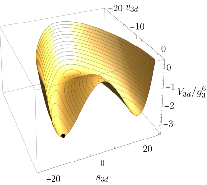
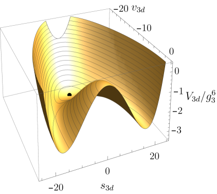
Figure 2: Schematic illustration for two-step phase transition, showcasing the effective potential near the critical temperature ($T_{{\mbox{\scriptsize c}},\phi}$) of the second phase transition from singlet to Higgs phase. At $T>T_{{\mbox{\scriptsize c}},\phi}$ (left), the minimum – depicted with a black dot – in singlet direction is global. At $T<T_{{\mbox{\scriptsize c}},\phi}$ (right), the Higgs phase becomes energetically favorable and the system undergoes a second phase transition. Since the singlet and Higgs minima are separated by a barrier, the transition is of first order. This barrier exists already at tree-level and therefore the second transition can be strong and relevant for gravitational wave production.

A sketch of the effective potential for a two-step phase transition [110, 111, 69, 49] is presented in fig. 2. It focuses on the second transition from singlet to Higgs phase. At higher temperatures, the extremum at the origin becomes the global minimum and the system is in the symmetric phase. In a first-order transition, the scalar condensates defined as [59]

$$\langle\phi^{\dagger}\phi\rangle \equiv\frac{\partial V^{{\mbox{\tiny\rm{eff}}}}_{{\mbox{\tiny\rm{3d}}}}}{\partial\mu^{2}_{3}}\;,$$ (2.15)

$$\langle S^{*}S\rangle \equiv 2\frac{\partial V^{{\mbox{\tiny\rm{eff}}}}_{{\mbox{\tiny\rm{3d}}}}}{\partial b_{2,3}}\;,$$ (2.16)

act in analogy to order parameters since they can be discontinuous at the critical temperature. The factor two in eq. (2.16) is a consequence of the chosen normalisation in eq. (2.1) for the singlet mass term. To measure the strength of the phase transition, we compute the latent heat $L=T\Delta p^{\prime}$. Here, the prime denotes a temperature derivative. In terms of the effective potential it reads

$$L(T) =T^{2}\Delta\frac{{\rm d}V^{{\mbox{\tiny\rm{eff}}}}_{{\mbox{\tiny\rm{3d}}}}}{{\rm d}T}\;.$$ (2.17)

In a naive perturbative treatment, the effective potential is simply minimised at different temperatures to find the phases, to determine the critical temperature and strength of the transition, as described above. However, this treatment leads to a subtlety related to gauge invariance: the value of the effective potential at its extrema, and therefore also at the minima, are gauge invariant. However, the minima themselves, i.e. values of the background fields, are gauge dependent. Furthermore, outside the extrema, the value of the effective potential is also gauge dependent and a numerical minimisation to find the minima of the potential inherits an artificial, residual gauge dependence of the gauge fixing parameters. Therefore, care has to be invested into this issue, as done in [66, 65, 71].

Gauge invariant computation

The Nielsen identities [67, 68] guarantee that the value of the effective potential in its minima are gauge invariant order-by-order in perturbation theory. In the $\hbar$-expansion [66, 65] orders of perturbation theory are tracked down in powers of a formal loop counting parameter. Additionally, the minima are expanded in $\hbar$ as: $v^{\text{min}}_{3}=v_{3,0}+\mathcal{O}(\hbar)$ and $s^{\text{min}}_{3}=s_{3,0}+\mathcal{O}(\hbar)$. Here $v_{3,0}$ and $s_{3,0}$ are the minima of the leading-order potential. During a second step of a two step transition, these are simply minima of the tree-level potential (cf. eqs. (3.5)–(3.7)) and the potential evaluated at the minima expands as

$$V^{{\mbox{\tiny\rm{eff}}}}_{{\mbox{\tiny\rm{3d}}}}(v^{{\mbox{\tiny\rm{min}}}}_{3},s^{{\mbox{\tiny\rm{min}}}}_{3}) =V^{{\mbox{\tiny\rm{tree}}}}_{{\mbox{\tiny\rm{3d}}}}(v_{3,0},s_{3,0})+\hbar\;V^{{\mbox{\tiny\rm{1-loop}}}}_{{\mbox{\tiny\rm{3d}}}}(v_{3,0},s_{3,0})+\mathcal{O}(\hbar^{2})\;.$$ (2.18)

The generic form of the $\mathcal{O}(\hbar^{2})$ correction can be found in [69], but we do not include it in our analysis as it requires a two-loop computation of $V^{{\mbox{\tiny\rm{eff}}}}_{{\mbox{\tiny\rm{3d}}}}$. At $\mathcal{O}(\hbar^{2})$ there would be additional contributions involving derivatives of the tree-level and one-loop pieces with respect to the background fields, as well as the two-loop potential itself. As we truncate our computation at $\mathcal{O}(\hbar)$, the only difference to the effective potential in terms of generic background fields is that we evaluate both tree-level and one-loop parts at the tree-level minima. In Fermi gauge and at one-loop level, the gauge fixing parameters appear solely in Goldstone mass eigenvalues $m_{1,\pm,3}$ and $m_{2,\pm,3}$ (eqs. (A.22) and (A.23)). These vanish at the tree-level minima $v_{3,0},s_{3,0}$ which in turn provides a gauge-invariant treatment at $\mathcal{O}(\hbar)$.

The procedure described above is improved compared to the PRM-scheme proposed in [65]. It consistently resums hard thermal loops (in 3d EFT parameters) to next-to-leading order (i.e. $\mathcal{O}(g^{4})$ in a formal power counting in $g$) while maintaining the gauge invariance. As described earlier, this ensures partial RG improvement related to the hard thermal scale with consistent resummation, and reduces the intrinsic uncertainty of the computation [63, 62]. In practice, we can find gauge-invariant critical temperatures in analogy to [65]: by determining values of the effective potential of eq. (2.18) in each minimum as function of temperature, and determining when the curves intersect (cf. fig. 3 (left)). On algorithm level [65], this is more efficient than the numerical minimisation of a complicated two- (or multi-) variate function. We also emphasise, that the condensates in eqs. (2.15)–(2.16) are gauge invariant when evaluated using eq. (2.18).

While gauge invariance is manifest in this treatment [66], one subtlety remains: radiatively generated or loop-induced transitions require additional care. In fact, for an expansion in $\hbar$ to be meaningful, the leading order minima $v_{3,0}$ and/or $s_{3,0}$ have to exist. For the $Z_{2}$-symmetric case (without mixing between scalar mass eigenstates) tree-level broken minima exist only if the (3d EFT) mass parameters become negative. In practice [69] this leads to a condition that the broken minima are global minima immediately when these mass parameters change sign. Therefore in this approach, solutions for the critical temperature are determined only from the condition that the corresponding 3d EFT mass parameter vanishes. This is not the physically correct picture. Another reason to be cautious, is that at two-loop order, the effective potential, or its derivatives related to gauge-invariant condensates, have a spurious IR divergence at a vanishing mass parameter which renders the computation further non-predictive [69]. Similarly, in the original ref. [66], an expression for the critical temperature itself was given in $\hbar$-expansion and found to diverge at $\mathcal{O}(\hbar^{2})$. Here, this problem haunts one-step transitions from the symmetric to the Higgs phase, as well as the first step of a two-step scenario from the symmetric to the singlet phase. For the latter, we further demonstrate this issue below for a concrete numerical example.

A cure of this technical problem is the resummation of a subset of one-loop contributions to the leading-order potential. Contributions from the heavy field give rise to a barrier at leading order (cf. eq. (2.14)). Consequently, minima of the leading-order potential are away from the point where the 3d EFT mass parameters vanish and the problematic IR behaviour described above can be avoided. However, as we only work with the leading-order potential for a radiatively generated first step of the transition, we are not able to directly demonstrate if higher order corrections are indeed free from spurious IR divergences. A related and detailed discussion on this topic can be found in [83].

3 Numerical analysis

To demonstrate numerically the setup for thermodynamics described in the previous section, we investigate a single parameter space point:

$$\Bigl{\{}\frac{m_{{\mbox{\tiny\rm{$H$}}}_{2}}}{\text{GeV}},\frac{m_{\mbox{\tiny\rm{$A$}}}}{\text{GeV}},\delta_{2},d_{2}\Bigr{\}}=\{62.5,62.5,0.55,0.5\}\;,$$ (3.1)

with $m_{{\mbox{\tiny\rm{$H$}}}_{1}}=125.1$ GeV identified with the observed Higgs boson mass. The pole masses of the other scalar bosons, $m_{{\mbox{\tiny\rm{$H$}}}_{2}}$ and $m_{\mbox{\tiny\rm{$A$}}}$, are related to $\overline{\text{MS}}$ parameters in appendix A.1, and the singlet portal coupling and self-interaction coupling are treated as input parameters. This parameter space point matches the S2 scenario studied in [39], and admits a two-step phase transition scenario. In fact, this point belongs to a subset of parameter space for which the tree-level potential eq. (2.1) is $Z_{2}$-symmetric $S\to-S$, viz. $a_{1}$ vanishes. In the same parameter space point also both the singlet VEV, $v_{S_{0}}$, and the mass parameter $b_{1}$ vanish. This simplifies the expressions in appendix A.1. For the replicability of the analysis, we explicitly write the $\overline{\text{MS}}$ parameters at the initial scale $M_{\mbox{\tiny\rm{$Z$}}}$:

$$\{g_{{\mbox{\tiny\rm{$Y$}}}}^{2},g_{\mbox{\scriptsize s}}^{2},g^{2},{g^{\prime}}^{2}\} =\{0.98,1.48,0.42,0.12\}\;,$$ (3.2)

$$\Bigl{\{}\frac{\mu^{2}_{h}}{\text{GeV}^{2}},\frac{b_{2}}{\text{GeV}^{2}},\frac{b_{1}}{\text{GeV}^{2}},\frac{a_{1}}{\text{GeV}^{3}}\Bigr{\}} =\{-7825,-8859,0,0\}\;,$$ (3.3)

$$\{\lambda_{h},\delta_{2},d_{2}\} =\{0.13,0.55,0.5\}\;,$$ (3.4)

which are obtained by solving the $\overline{\text{MS}}$ parameters as a function of the input parameters of eq. (3.1) using the relations of appendix A.1. Here, we displayed rounded up numbers while our analysis uses higher decimal accuracy.

For comparison, we describe below both the gauge in- and dependent determinations of our numerical analysis. It proceeds in the following steps:

• For a fixed input parameter space point, solving the $\overline{\text{MS}}$ parameters by tree-level relations (cf. appendix A.1).

• Solving RG running of the $\overline{\text{MS}}$ parameters from the one-loop beta-functions (cf. appendix A.2).

• For fixed temperature $T$, the parameters of the 3d EFT are obtained from the matching relations of appendix A.4 in terms of the $\overline{\text{MS}}$ parameters that are run to a chosen $T$-dependent scale.

• For fixed temperature $T$, the thermal effective potential within the 3d EFT is constructed as described in the previous section either in the gauge-invariant $\hbar$-expansion at leading order minima, or in Fermi gauge as a function of generic background fields.

• Steps 3 and 4 are repeated for different values of $T$ and critical temperatures $T_{\rm c}$, condensates and latent heat are determined, as described in the previous section. We further demonstrate this in figures below in this section.

Partial RG improvement (related to the hard thermal scale) manifests through steps 2 and 3, when the 4d RG scale cancels at $\mathcal{O}(g^{4})$. Unlike in [39], where running is only implemented to the tree-level part of the effective potential, we use running couplings consistently everywhere. This will induce contributions that are formally of higher order than the accuracy of our computation. In spirit of [112, 113, 63, 62, 2, 114], this indicates the intrinsic uncertainty of our analysis. We emphasise that, in a consistent cancellation of 4d RG scale at $\mathcal{O}(g^{4})$, two-loop pieces of 3d mass parameters – or two-loop thermal masses – are essential [62].

This technical detail has been overlooked by all existing literature on the cxSM thermodynamics. Our computation is the first one to account and demonstrate the importance of this partial RG improvement. By working at $\mathcal{O}(\hbar)$ or one-loop within the 3d perturbation theory, we do not have full, consistent leading RG improvement at $\mathcal{O}(g^{4})$. However, we can estimate the magnitude of the missing two-loop contributions by including the 3d running of mass parameters and varying the corresponding 3d RG scale.

The gauge invariance of our analysis is guaranteed by the gauge-invariant matching relations of step 3 and the $\hbar$-expansion in step 4. For comparison, we also perform the gauge-dependent analysis in the Landau gauge which has been one of the most common choices in the literature for the EWPT in different BSM extensions.

Critical temperature

We first determine the different phases as a function of temperature from the value of the effective potential at different local minima of the leading-order potential. For our benchmark point, the formulae of the tree-level minima admit a simple closed form:

symmetric phase: $$\qquad\Bigl{\{}v_{3,0}=0,s_{3,0}=0\Bigr{\}}\;,$$ (3.5)

singlet phase: $$\qquad\Bigl{\{}v_{3,0}=0,s_{3,0}=-i\;\sqrt{\frac{2b_{2,3}}{d_{2,3}}}\Bigr{\}}\;,$$ (3.6)

Higgs phase: $$\qquad\Bigl{\{}v_{3,0}=-i\;\sqrt{\frac{\mu^{2}_{h,3}}{\lambda_{h,3}}},s_{3,0}=0\Bigr{\}}\;.$$ (3.7)

In other parameter space points, that are not considered here, solutions for minima can be functionally more complicated. In terms of the above expressions, we denote

$$V^{\text{sym}}_{\text{eff}} \equiv V^{\text{3d}}_{\text{eff}}(0,0)\;,$$ (3.8)

$$V^{S}_{\text{eff}} \equiv V^{\text{3d}}_{\text{eff}}\biggl{(}0,-i\sqrt{\frac{2b_{2,3}}{d_{2,3}}}\biggr{)}\;,$$ (3.9)

$$V^{\phi}_{\text{eff}} \equiv V^{\text{3d}}_{\text{eff}}\biggl{(}-i\sqrt{\frac{\mu^{2}_{h,3}}{\lambda_{h,3}}},0\biggr{)}\;.$$ (3.10)

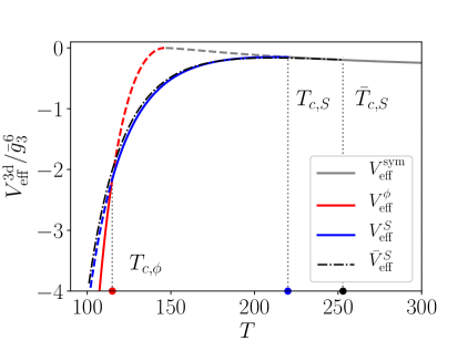
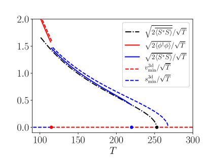
Figure 3: Left: Value of the effective potential as function of temperature $T$ in the symmetric (grey), Higgs (red) and singlet (blue) phase. Solid lines illustrate the global minimum. For dashed lines the potential also develops an imaginary part, signalling that the corresponding phase is not a stable minimum. Each phase is present only at limited $T$-intervals. Outside these ranges, the value of the effective potential is purely imaginary. Critical temperatures are determined from the intersection points, illustrated by dotted vertical lines and dots on the $x$-axis. The dotted-dashed black line describes the singlet phase in the EFT setup with a radiative barrier from the heavy Higgs. Right: The solid blue and red lines show the square root of the gauge-invariant singlet and Higgs condensates in a temperature range for which they are real. The dotted-dashed black line presents the singlet condensate, in heavy Higgs EFT, in analogy to the left panel. For comparison, the dashed lines show the gauge-dependent values of the background fields in the global minima of the Landau gauge effective potential.

The left panel of fig. 3 plots these expressions as a function of the temperature (cf. similar fig. 3 in [65]). In this figure, we present the value of the effective potential in units of $g^{6}_{3}$; the gauge coupling squared has dimension of mass in the 3d EFT. Further, we used fixed RG scales $\mu=1.25\pi T$ and $\mu_{3}=g^{2}_{3}$. Later in this section, we investigate how results change by varying these arbitrary RG scales.

The intersection points of $V^{\text{sym}}_{\text{eff}}$, $V^{S}_{\text{eff}}$, and $V^{\phi}_{\text{eff}}$ determine critical temperatures. On algorithmic level, finding intersections of these curves is significantly faster than minimising the (gauge-dependent) effective potential which is a function of two variables. Since $V^{\text{sym}}_{\text{eff}}$ and $\bar{V}^{\text{sym}}_{\text{eff}}$ are numerically indiscernible within the chosen plot ranges, we do not visualise $\bar{V}^{\text{sym}}_{\text{eff}}$.

The global minimum is easily identified with the lowest value and we denote it by a solid line, while dashed lines indicate that each local minimum is no longer the global one. Each of the three minima are global in turn, signalling a two-step phase transition. The intersection points of the global minima reveal the critical temperatures – illustrated by vertical lines – for both phase transitions. As already discussed above, the determination of the critical temperature of the first transition, $T_{{\mbox{\scriptsize c}},S}$, is cumbersome as only after this point (i.e. at lower temperature) the singlet minimum exists (at higher temperature $V^{S}_{\text{eff}}$ has an imaginary value), and $T_{{\mbox{\scriptsize c}},S}$ is therefore determined by the condition $b_{2,3}(T_{{\mbox{\scriptsize c}},S})=0$. This would lead to an IR divergence for the singlet condensate already at two-loop level [66, 69] (also cf. [115]), and further signals that interpreting this point as the physical critical temperature is incorrect. The physically correct picture is provided by solving the broken singlet minimum $\bar{s}_{3,0}$ from eq. (2.14), i.e.

$$\frac{{\rm d}}{{\rm d}s_{3}}V^{\text{eff,rb}}(s_{3})=0\;,$$ (3.11)

at $s_{3}=\bar{s}_{3,0}$. This equation has four different solutions for the broken phase extrema $\bar{s}_{3,0}\neq 0$ and in the case of interest, the broken minimum is described by

$$\bar{s}_{3,0} =\frac{1}{2\pi\sqrt{2}}\Bigl{[}\frac{1}{d^{2}_{2,3}}\Bigl{(}\delta^{3}_{2,3}-(4\pi)^{2}(b_{1,3}+b_{2,3})d_{2,3}$$

$$-\delta_{2,3}\sqrt{\delta^{4}_{2,3}+(4\pi)^{2}\bigl{(}-2(b_{1,3}+b_{2,3})d_{2,3}\delta_{2,3}+4\mu^{2}_{S,3}d^{2}_{2,3}\bigr{)}}\Bigr{)}\Bigr{]}^{\frac{1}{2}}\;.$$ (3.12)

For a radiatively generated barrier, the functional forms for the different extrema become seemingly more complicated. However, the minimum at each temperature can still be identified by a derivative test of a single-variable function. We define the notation $\bar{V}^{\text{S}}_{\text{eff}}\equiv V^{\text{eff,rb}}(\bar{s}_{3,0})$ and $\bar{V}^{\text{sym}}_{\text{eff}}\equiv V^{\text{eff,rb}}(0)$. The critical temperature $\bar{T}_{{\mbox{\scriptsize c}},S}$ is determined from the temperature value when $\bar{V}^{\text{S}}_{\text{eff}}$ becomes real and $\bar{V}^{\text{S}}_{\text{eff}}<\bar{V}^{\text{sym}}_{\text{eff}}$. Since $\bar{T}_{{\mbox{\scriptsize c}},S}$ is different from $T_{{\mbox{\scriptsize c}},S}$ in which $\mu^{2}_{S,3}=0$, the former solution for the critical temperature does not necessarily lead to spurious IR divergences for condensates or latent heat at higher loop levels.

Gauge invariant condensates

The gauge-invariant condensates are analogous to order parameters such that for a first-order phase transition they are discontinuous at the critical temperature. As an analogy to a typical gauge-dependent analysis in terms of gauge-dependent background fields, we investigate the expressions [113, 64]

$$\frac{v_{\text{phys}}}{T}\equiv\frac{\sqrt{2\langle\phi^{\dagger}\phi\rangle}}{\sqrt{T}}\;,$$ (3.13)

$$\frac{s_{\text{phys}}}{T}\equiv\frac{\sqrt{2\langle S^{*}S\rangle}}{\sqrt{T}}\;.$$ (3.14)

The condensates have discontinuities at the critical temperatures, and the Higgs (singlet) condensate is negative outside of the Higgs (singlet) phase. Therefore these expressions are imaginary outside of their respective phase. In fig. 3 (right) we plot the expressions of eqs. (3.13) and (3.14) as a function of temperature (solid lines). For the singlet condensate, we plot the result computed both from $V^{\text{S}}_{\text{eff}}$ and $\bar{V}^{\text{S}}_{\text{eff}}$. For the latter, we denote $\overline{\langle S^{*}S\rangle}\equiv 2\frac{\partial\bar{V}^{\text{S}}_{\text{eff}}}{\partial b_{2,3}}$ and witness that sufficiently below $\bar{T}_{{\mbox{\scriptsize c}},S}$ these results overlap until a second phase transition. We fixed RG scales at $\mu=1.25\pi T$ and $\mu_{3}=g^{2}_{3}$.

The same plot presents the gauge-dependent background fields at the global minima of the effective potential (eq. (2.10)) in Landau gauge $\xi_{1}=\xi_{2}=0$ (dashed lines). From this comparison, we observe that outside of the critical temperature of the first transition, both approaches agree rather well. We interpret this as an echo of common lore in the literature (cf. e.g. [112]) that the Landau gauge results – albeit inherently gauge-dependent, and therefore unphysical – are numerically close to gauge-invariant results, perhaps encouraging their use as a practical guide.

On purely theoretical grounds, gauge-dependent predictions for physical quantities are unsatisfactory and inherently incorrect. Hence, it is invaluable to develop and use a theoretically sound technique to analyse phase transition thermodynamics. The Landau gauge results have been hoped to be useful in practice, with the expectation that the error related to unphysical gauge dependence is smaller than other uncertainties of the problem (cf. discussion on varying renormalisation scales below). However, the gauge fixing parameter is still an arbitrarily valued input. In practice, larger values could lead to larger numerical errors additional to the theoretical blemish.

Latent heat and renormalisation scale dependence

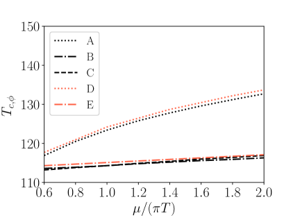
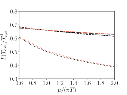
Figure 4: Left: $T_{{\mbox{\scriptsize c}},\phi}$ as function of the 4d renormalisation scale $\mu$ in different approximations (A–E) that are detailed in the main body. The gauge-invariant $\hbar$-expansion (black lines A, B, C) and the analysis based on direct numerical minimisation of the effective potential in Landau gauge (grey lines D, E) show minor difference in the sensitivity to $\mu$. Right: As left panel, but for the latent heat evaluated at $T_{{\mbox{\scriptsize c}},\phi}$.

The accuracy of our analysis is investigated by varying the input renormalisation scales, similar to recent studies [63, 62]. The left panel of fig. 4 plots $T_{{\mbox{\scriptsize c}},\phi}$ – the critical temperature of the second transition – as a function of the 4d RG scale $\mu$. Similarly, fig. 4 (right) evaluates the latent heat at $T_{{\mbox{\scriptsize c}},\phi}$. We show five different lines: lines A, B and C (black) are based on the gauge-invariant $\hbar$-expansion while lines D and E (red) use a direct numerical minimisation of the effective potential in Landau gauge. Similar to fig. 3 (right), the two methods agree closely. Concretely the lines contain:

• one-loop level dimensional reduction,

• two-loop level dimensional reduction,

• as B, with varying $\mu_{3}=(\frac{\mu}{\pi T})g^{2}_{3}$.

The difference between the two levels of accuracy in dimensional reduction arises from two-loop contributions to the thermal masses. By comparison, we observe that without two-loop thermal masses, the results are strongly RG scale-dependent. As reviewed in sec. 2, the two-loop logarithmic terms compensate the leading running of the one-loop thermal corrections to the mass parameters in quadratic terms [62]. If these two-loop contributions are omitted, the resulting uncertainty completely overshadows the ambiguity related to the numerical difference of gauge-invariant and gauge-dependent (Landau gauge) approaches. Finally, along the black dashed line C, we also varied the 3d RG scale $\mu_{3}$ (whereas for other lines it is fixed $\mu_{3}=g^{2}_{3}$). This variation signals the importance of two-loop contributions at $\mathcal{O}(\hbar^{2})$ within 3d perturbation theory that we omitted in eq. (2.18). Note that mass parameters of the 3d EFT are running in terms of this 3d scale and logarithms of the 3d RG scale only appear at two-loop order. While this effect is significantly smaller than two-loop contributions from the hard thermal scale to the mass parameters, it still causes a sizable uncertainty. This motivates to increase the accuracy to $\mathcal{O}(\hbar^{2})$ in future computations.

4 Discussion

The method presented in this article for phase transition thermodynamics avoids the triune poison of gauge dependence, slow convergence of perturbation theory and intractability. Our investigation follows [66, 69, 63, 62] and implements thermal resummations related to the hard thermal scale of non-zero Matsubara modes using the dimensionally reduced 3d EFT. It further used the gauge-invariant $\hbar$-expansion within 3d perturbation theory to compute the thermodynamic quantities pertinent to electroweak phase transitions. In analogy to previous studies [63, 62], we find alarming sensitivity to the renormalisation scale at one-loop level and we identified two-loop thermal masses to be the most crucial contributions to reduce this RG scale dependence. Their importance was previously highlighted in [62]. We note that these findings are in contrast to [80].

Thus, we suggest a minimal setup for perturbative accuracy, that still eliminates most of the undesired scale dependence. It combines NLO dimensional reduction including two-loop thermal masses and a one-loop effective potential in the 3d EFT with a simple expression in terms of the background field dependent mass eigenvalues. The difference to [69, 116, 64, 62] is that the two-loop effective potential in 3d EFT is not included; the RG improvement related to hard thermal scale can still be acquired. The described setup relies on the ability to construct the 3d EFT matching relations by dimensional reduction. Such a setup is, unfortunately, still rare in current BSM EWPT literature. To this end, we expect upcoming automated software [91] – designated for this problem – to increase the applicability of improved studies based on the 3d EFT. We further comment that ref. [29] has attempted to improve resummation of hard thermal loops and in particular to compute thermal masses beyond leading order based on “partial dressing” [117] but without using high-temperature expansion nor dimensional reduction to 3d EFT. Another computation of the two-loop thermal effective potential without high-temperature expansion appears in [113] (cf. also [118]).

The results of our gauge-invariant computation do not differ drastically numerically from conventional Landau gauge analyses. Such a difference is completely overshadowed in a mere one-loop analysis by the uncertainty from the renormalisation scale. This, however, supports the common wisdom that while a gauge-invariant computation is theoretically important, it should not come at the expense of resummation and including relevant terms in the coupling expansion. In part, a similar conclusion was reached in [71]. In this regard, our computation significantly improves the previously suggested PRM scheme [65] by incorporating the required resummations consistently, while maintaining gauge invariance.

Finally, for the cxSM, the questions studied in [39, 80] could benefit from the tools presented in this article. In particular, by focusing on what can be concluded about the possible thermal history of EWSB in this scenario, when both gauge invariance and RG improvement are installed. The presented tools can be used for wide scans of the model parameter space and to analyse physical implications. The latter can shed light on which regions of parameter space admit both a strong first-order phase transitions and dark matter candidates and what are the collider phenomenology signatures of these regions. In addition to the improved equilibrium thermodynamics computation of this article, future scans would benefit from a two-loop effective potential in 3d perturbation theory, as well as from the one-loop improved (zero-temperature) relations between $\overline{\text{MS}}$ parameters and physical input parameters. Both of these improvements are available in the real singlet-extended Standard Model (xSM) collected in appendices A and B of [64] and could be generalised to the cxSM.

A further computation of the bubble nucleation rate is required for studying the gravitational wave production in the cxSM. Therefore, one can combine the 3d EFT presented in this article with recent technology [72]. In general, the same approach applies to other BSM theories and in particular those with extended scalar sector.

Appendix A Collected formulae

This appendix collects several formulae that connect the input parameters of eq. (3.1) to the effective potentials in eqs. (2.10) and (2.14). We also collect numerical results for the thermodynamics presented by the figures in sec. 3.

A.1 Relations between $\overline{\text{MS}}$ parameters and input parameters

In the gauge and Yukawa sector, we use input values [119]

$$\{M_{\mbox{\tiny\rm{$W$}}},M_{\mbox{\tiny\rm{$Z$}}},M_{t}\}=\{80.379~{}{\rm GeV},91.1876~{}{\rm GeV},172.76~{}{\rm GeV}\}\;,$$ (A.1)

together with the strong coupling $g_{\mbox{\scriptsize s}}=1.48409$ and the reduced Fermi constant $G_{\mbox{\scriptsize F}}=1.1663787\times 10^{-5}~{}{\rm GeV}^{-2}$. The strong coupling enters the two-loop thermal mass for Higgs doublet. Using the shorthand notation $g^{2}_{0}\equiv 4\sqrt{2}G_{\mbox{\scriptsize F}}M_{\mbox{\tiny\rm{$W$}}}^{2}$, we have

$$g^{2} =g^{2}_{0}\;,\quad\quad{g^{\prime}}^{2}=g^{2}_{0}\Big{(}\frac{M_{\mbox{\tiny\rm{$Z$}}}^{2}}{M_{\mbox{\tiny\rm{$W$}}}^{2}}-1\Big{)}\;,\quad\quad g_{{\mbox{\tiny\rm{$Y$}}}}^{2}=\frac{1}{2}g^{2}_{0}\frac{M^{2}_{t}}{M_{\mbox{\tiny\rm{$W$}}}^{2}}\;,\quad\quad v_{0}=\sqrt{\frac{4M_{\mbox{\tiny\rm{$W$}}}^{2}}{g^{2}_{0}}}\;.$$ (A.2)

To relate the $\overline{\text{MS}}$ parameters to the above input parameters, we use analytic, tree-level relations

$$b_{1} =m^{2}_{{\mbox{\tiny\rm{$H$}}}_{2}}-m_{\mbox{\tiny\rm{$A$}}}^{2}\;, b_{2} =m^{2}_{{\mbox{\tiny\rm{$H$}}}_{2}}+m_{\mbox{\tiny\rm{$A$}}}^{2}-\frac{1}{2}v^{2}_{0}\delta_{2}\;,$$

$$\mu^{2}_{h} =-\frac{1}{2}m^{2}_{{\mbox{\tiny\rm{$H$}}}_{1}}\;, \lambda_{h} =\frac{1}{2}\frac{m^{2}_{{\mbox{\tiny\rm{$H$}}}_{1}}}{v^{2}_{0}}\;.$$ (A.3)

In many other parameter space points, the relations between $\overline{\text{MS}}$ parameters and input parameters do not have such simple analytic relations for non-vanishing $a_{1}$, $v_{S_{0}}$ and the mixing angle $\alpha$. In these cases, one can solve the $\overline{\text{MS}}$ parameters numerically by inverting the mass eigenvalues ($m_{+}$ is identified with $m_{{\mbox{\tiny\rm{$H$}}}_{2}}$ and $m_{-}$ with $m_{{\mbox{\tiny\rm{$H$}}}_{1}}$), together with the tadpole conditions

$$v_{0}\Big{(}\mu_{h}^{2}+\lambda_{h}v^{2}_{0}+\frac{1}{4}\delta_{2}v^{2}_{S_{0}}\Big{)} =0\;,$$ (A.4)

$$\sqrt{2}a_{1}+\frac{1}{2}(b_{1}+b_{2})v_{S_{0}}+\frac{1}{4}d_{2}v_{0}^{3}+\frac{1}{4}\delta_{2}v_{0}^{2}v_{S_{0}} =0\;,$$ (A.5)

and the equation for the mixing angle

$$\cot(2\alpha) =-\bigg{(}\frac{-4\mu^{2}_{h}+2(b_{1}+b_{2})+(3d_{2}-\delta_{2})v^{2}_{S_{0}}+(\delta_{2}-12\lambda_{h})v^{2}_{0}}{4\delta_{2}v_{0}v_{S_{0}}}\bigg{)}\;.$$ (A.6)

All above relations hold at tree-level and receive quantum corrections in zero-temperature perturbation theory. In a consistent power counting up to $\mathcal{O}(g^{4})$, one would need to include one-loop corrections to relations of $\overline{\text{MS}}$ and physical parameters (cf. [58, 113, 109, 44, 64]) – we do not include them here. Due to this omission we do not have the proper initial conditions in our partial RG-improvement at $\mathcal{O}(g^{4})$. However, our discussion remains qualitatively intact as these initial conditions merely shift the corresponding benchmark point in the $\overline{\text{MS}}$ parameter space. Once this point is carefully related to particle collider phenomenology constraints, the improved initial conditions become quantitatively relevant to be accounted for.

A.2 Renormalisation group equations

By parametrising the $\overline{\text{MS}}$ renormalization scale through $t=\ln\mu^{2}$ the one-loop $\beta$-functions, or renormalisation group equations, for the $\overline{\text{MS}}$ parameters read

$$\partial_{t}\lambda_{h} =\beta_{{\mbox{\tiny\rm{SM}}}}(\lambda_{h})+\frac{1}{(4\pi)^{2}}\Big{(}\frac{1}{8}\delta^{2}_{2}\Big{)}\;,$$ (A.7)

$$\partial_{t}d_{2} =\frac{1}{(4\pi)^{2}}\Big{(}\frac{5}{2}d^{2}_{2}+\delta^{2}_{2}\Big{)}\;,$$ (A.8)

$$\partial_{t}\delta_{2} =\frac{1}{(4\pi)^{2}}\delta_{2}\Big{(}d_{2}+\delta_{2}+6\lambda_{h}-\frac{3}{4}(3g^{2}+{g^{\prime}}^{2})+3g_{{\mbox{\tiny\rm{$Y$}}}}^{2}\Big{)}\;,$$ (A.9)

$$\partial_{t}\mu^{2}_{h} =\beta_{{\mbox{\tiny\rm{SM}}}}(\mu^{2}_{h})+\frac{1}{(4\pi)^{2}}\Big{(}\frac{1}{4}b_{2}\delta_{2}\Big{)}\;,$$ (A.10)

$$\partial_{t}b_{2} =\frac{1}{(4\pi)^{2}}\Big{(}b_{2}d_{2}+2\delta_{2}\mu_{h}^{2}\Big{)}\;,$$ (A.11)

$$\partial_{t}b_{1} =\frac{1}{(4\pi)^{2}}\Big{(}\frac{1}{2}b_{1}d_{2}\Big{)}\;.$$ (A.12)

In the beta-functions for $\mu^{2}_{h}$ and $\lambda_{h}$, we depict explicitly only the new complex singlet contributions; pure SM contributions are collected in e.g. [88].

A.3 Mass eigenvalues for background field method

Parametrising doublet and singlet fields in analogy to eq. (2.2), but replacing zero-temperature VEVs, $v_{0}$ and $v_{S_{0}}$ by generic, real background fields $v$ and $s$ results in mass eigenvalues for the background field method

$$m^{2}_{\chi} =\mu^{2}_{h}+\lambda_{h}v^{2}+\frac{1}{4}\delta_{2}s^{2},$$ (A.13)

$$m_{\mbox{\tiny\rm{$A$}}}^{2} =\frac{1}{2}(-b_{1}+b_{2})+\frac{1}{4}d_{2}s^{2}+\frac{1}{4}\delta_{2}v^{2}\;,$$ (A.14)

$$m^{2}_{\pm} =\frac{1}{4}\bigg{\{}2\mu^{2}_{+}b_{1}+b_{2}+(6\lambda_{h}+\frac{1}{2}\delta_{2})v^{2}+\frac{1}{2}(\delta_{2}+3d_{2})s^{2}$$

$$\pm\frac{1}{2}\sqrt{c_{1}+c_{2}v^{4}+c_{3}s^{4}+c_{4}v^{2}+c_{5}s^{2}+c_{6}v^{2}s^{2}}\bigg{\}}\;,$$ (A.15)

where we used the shorthand notation

$$c_{1} =4(b_{1}+b_{2}-2\mu^{2}_{h})^{2}\;,$$ (A.16)

$$c_{2} =(\delta_{2}-12\lambda_{h})^{2}\;,$$ (A.17)

$$c_{3} =(\delta_{2}-3d_{2})^{2}\;,$$ (A.18)

$$c_{4} =4(\delta_{2}-12\lambda_{h})(b_{1}+b_{2}-2\mu^{2}_{h})\;,$$ (A.19)

$$c_{5} =-4(\delta_{2}-3d_{2})(b_{1}+b_{2}-2\mu^{2}_{h})\;,$$ (A.20)

$$c_{6} =6d_{2}(\delta_{2}-12\lambda_{h})+2\delta_{2}(7\delta_{2}+12\lambda_{h})\;.$$ (A.21)

These mass eigenvalues, in terms of parameters of the 4d parent theory (2.1), can be inverted to obtain the tree-level relations between $\overline{\text{MS}}$ parameters and physical masses in appendix A.1.

When computing the effective potentials in the 3d EFT, eqs. (2.10) and (2.14), we denote background field dependent mass eigenvalues by an additional subscript 3. Then all parameters and background fields therein are those of the 3d EFT. In addition, when computing the effective potential in Fermi gauge, Goldstone mass eigenvalues $m^{2}_{\chi}$ are replaced by [120]

$$m^{2}_{1,\pm} =\frac{1}{2}\Big{(}m^{2}_{\chi}\pm\sqrt{m^{2}_{\chi}\big{(}m^{2}_{\chi}-v^{2}(g^{2}\xi_{2}+{g^{\prime}}^{2}\xi_{1})\big{)}}\Big{)}\;,$$ (A.22)

$$m^{2}_{2,\pm} =\frac{1}{2}\Big{(}m^{2}_{\chi}\pm\sqrt{m^{2}_{\chi}\big{(}m^{2}_{\chi}-v^{2}g^{2}\xi_{2}\big{)}}\Big{)}\;,$$ (A.23)

where $m^{2}_{2,\pm}$ are double-degenerate. The singlet does not contribute to mass eigenvalues for weak bosons, viz.

$$m_{\mbox{\tiny\rm{$W$}}}^{2} =\frac{1}{4}g^{2}v^{2}\;,\quad m_{\mbox{\tiny\rm{$Z$}}}^{2}=\frac{1}{4}(g^{2}+{g^{\prime}}^{2})v^{2}\;,$$ (A.24)

and the mass eigenvalue for the photon vanishes.

A.4 Matching relations for dimensional reduction

We define a shorthand notation

$$L_{b} \equiv 2\ln\Big{(}\frac{\mu}{T}\Big{)}-2\Big{(}\ln(4\pi)-\gamma\Big{)}\;,$$ (A.25)

$$c =\frac{1}{2}\Bigl{(}\ln\Big{(}\frac{8\pi}{9}\Big{)}+\frac{\zeta_{2}^{\prime}}{\zeta_{2}}-2\gamma\Bigr{)}\;,$$ (A.26)

where $\zeta_{s}$ for $\Re\,(s)>1$ is the Riemann Zeta function. Matching relations between parent 4d theory and 3d EFT read

$$\lambda_{h,3} =\lambda_{h,3,{\mbox{\tiny\rm{SM}}}}+T\frac{L_{b}}{(4\pi)^{2}}\Big{(}-\frac{1}{8}\delta^{2}_{2}\Big{)}\;,$$ (A.27)

$$d_{2,3} =T\Big{(}d_{2}(\mu)-\frac{L_{b}}{(4\pi)^{2}}\Big{(}\frac{5}{2}d^{2}_{2}+\delta^{2}_{2}\Big{)}\Big{)}\;,$$ (A.28)

$$\delta_{2,3} =T\Big{(}\delta_{2}(\mu)-\frac{L_{b}}{(4\pi)^{2}}\delta_{2}\Big{(}d_{2}+\delta_{2}+6\lambda_{h}-\frac{3}{4}(3g^{2}+{g^{\prime}}^{2})\Big{)}$$

$$\hphantom{{}=T\Big{(}\delta_{2}(\mu)}-\frac{L_{f}}{(4\pi)^{2}}\delta_{2}\Big{(}3g_{{\mbox{\tiny\rm{$Y$}}}}^{2}\Big{)}\Big{)}\;,$$ (A.29)

$$\mu^{2}_{h,3}(\mu_{3}) =\mu^{2}_{h,3,{\mbox{\tiny\rm{SM}}}}+\frac{1}{24}T^{2}\delta_{2}(\mu)-\frac{L_{b}}{(4\pi)^{2}}\Big{(}\frac{1}{4}b_{2}\delta_{2}\Big{)}$$

$$+\frac{1}{(4\pi)^{2}}T^{2}\frac{\delta_{2}}{24}\Big{(}\frac{3}{4}(3g^{2}+{g^{\prime}}^{2})L_{b}-3g_{{\mbox{\tiny\rm{$Y$}}}}^{2}L_{f}\Big{)}$$

$$-\frac{T^{2}L_{b}}{(4\pi)^{2}}\delta_{2}\Big{(}\frac{1}{24}d_{2}+\frac{5}{48}\delta_{2}+\frac{1}{4}\lambda_{h}\Big{)}$$

$$+\frac{1}{(4\pi)^{2}}T^{2}\Big{(}-\frac{1}{4}\delta^{2}_{2}\Big{)}\Big{(}c+\ln\Big{(}\frac{3T}{\mu_{3}}\Big{)}\Big{)}\;,$$ (A.30)

$$b_{2,3}(\mu_{3}) =b_{2}(\mu)+\frac{1}{6}T^{2}\Big{(}d_{2}(\mu)+\delta_{2}(\mu)\Big{)}-\frac{L_{b}}{(4\pi)^{2}}\Big{(}b_{2}d_{2}+2\delta_{2}\mu_{h}^{2}\Big{)}$$

$$+\frac{T^{2}}{(4\pi)^{2}}\frac{\delta_{2}}{12}\Big{(}3g^{2}+{g^{\prime}}^{2}+3g_{{\mbox{\tiny\rm{$Y$}}}}^{2}L_{f}\Big{)}$$

$$+\frac{T^{2}L_{b}}{(4\pi)^{2}}\Big{(}-\frac{5}{12}d^{2}_{2}-\frac{1}{6}d_{2}\delta_{2}+\frac{3}{8}g^{2}\delta_{2}+\frac{1}{8}{g^{\prime}}^{2}\delta_{2}-\frac{3}{4}g_{{\mbox{\tiny\rm{$Y$}}}}^{2}\delta_{2}-\frac{1}{3}\delta_{2}^{2}-\delta_{2}\lambda_{h}\Big{)}$$

$$+\frac{1}{(4\pi)^{2}}T^{2}\Big{(}-d^{2}_{2}-\delta^{2}_{2}+(3g^{2}+{g^{\prime}}^{2})\delta_{2}\Big{)}\Big{(}c+\ln\Big{(}\frac{3T}{\mu_{3}}\Big{)}\Big{)}\;,$$ (A.31)

$$b_{1,3} =b_{1}(\mu)+\frac{L_{b}}{(4\pi)^{2}}\Big{(}-\frac{1}{2}b_{1}d_{2}\Big{)}\;,$$ (A.32)

$$a_{1,3} =\frac{1}{\sqrt{T}}a_{1}\;.$$ (A.33)

Here, we explicitly suppress pure SM contributions since they can be found e.g. in [81] together with the matching relations for the 3d gauge couplings and parameters of the temporal sector. The tutorial of [81] also computes similar matching relations for a real singlet field. The tadpole coupling $a_{1,3}$ does not receive loop corrections since cubic couplings are absent.

All matching relations eqs. (A.27)–(A.33) are gauge invariant. By computing the matching in Fermi gauge, we could demonstrate an exact cancellation of the gauge fixing parameters (cf. similarly [63, 81, 73]).

Appendix B Renormalisation group improvement

At high temperature, the running with respect to the 4d RG scale $\mu$, described by beta-functions $\beta(g^{2})$, is not altered compared to zero temperature. However, an overall RG improvement for the effective potential at high temperature is more subtle because thermal scale hierarchies reflect to the structure of the potential [60, 62]. In the mapping between 4d and 3d EFT (cf. sec. A.4), the 4d RG scale $\mu$ cancels between LO running and explicit logarithms within the $L_{b}$-terms at NLO in the matching relations of the 3d parameters. This corresponds to cancellation of the RG scale related to hard mode contributions in eq. (2.6).

In the 3d EFT perturbation theory constitutes another, independent, renormalisation scale $\mu_{3}$. Without higher dimensional operators that appear at $\mathcal{O}(g^{6})$, the 3d EFT is super-renormalisable. Hence, counterterms in dimensional regularisation have a finite number of terms sufficient to cancel all UV divergences at any loop order. In the SM – and many of its extensions – only the mass parameters (or tadpole parameters) require renormalisation. The 3d couplings are RG invariant and the mass counterterms are exact already at two-loop order. This gives rise to the exact running of mass parameters in terms of $\mu_{3}$. Since the running of the mass appears at two-loop order, the cancellation of $\mu_{3}$ in eq. (2.6) leap frogs over even and odd terms. The running of $g^{2}$-terms cancels logarithms at $g^{4}$-terms, and the running of $g^{3}$-terms cancels logarithms at $g^{5}$-terms and so forth.

In this context, the discussion in ref. [39] on the RG improvement of the cxSM is incomplete. Therein, the one-loop effective potential is divided into a tree-level piece, the zero-temperature Coleman-Weinberg (CW) potential, and the one-loop thermal function. Consequently, the parameters in the tree-level potential are replaced by the parameters solved from one-loop RGEs which correctly eliminates the explicit logarithmic RG scale dependence in the CW potential. Contrary to [39] the renormalization scale does enter the high-$T$ effective potential. While it is true that the one-loop thermal function is not explicitly dependent on the renormalisation scale, there is still an implicit running of the parameters inside the thermal function. The latter, contributes at same order as running of tree-level potential. Crucially, should one implement high temperature expansion to this thermal function, it is straightforward to observe that its leading behaviour of the quadratic terms – that contribute to one-loop thermal masses – is of same order in formal power counting as tree-level terms, i.e. $\mathcal{O}(g^{2})$. The running of the one-loop thermal mass contributions is therefore an effect of $\mathcal{O}(g^{4})$ and this running is cancelled by logarithmic terms for thermal masses that appear at two-loop order. It is indeed these contributions that we include in our analysis with a NLO dimensional reduction. We also demonstrated their crucial importance in our numerical analysis of sec. 3.

Appendix Epilogue Standard Model with a light Higgs

As an illuminating example, we discuss how even in the pure SM the running of the one-loop thermal mass can cause an alarming leftover scale dependence if the full two-loop thermal mass is not computed. For illustration, we work with a toy model of a pure SM (i.e. we omit complex singlet contributions from the dimensional reduction and 3d EFT of earlier sections) and we vary the Higgs mass in $m_{h}=(50\dots 130)$ GeV. For simplicity, we determine the critical temperature $T_{\rm c}$ from the condition that the minima of the one-loop effective potential in 3d EFT are degenerate. We use the ratio $\phi_{{\mbox{\scriptsize c}}}/T_{\rm c}$ as an estimate of the transition strength. By doing so, we provide an analogy to many BSM studies that analyse the electroweak phase transition simply in Landau gauge in terms of the gauge-dependent $T_{\rm c}$ and $\phi_{{\mbox{\scriptsize c}}}/T_{\rm c}$. In fig. 5 we depict these quantities as a function of the Higgs mass.

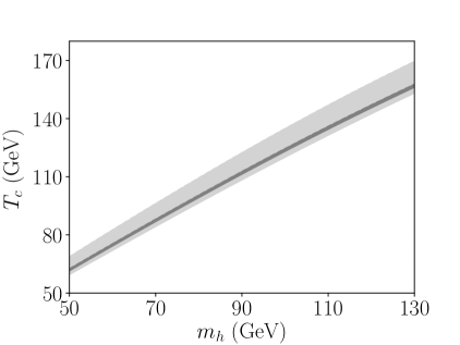
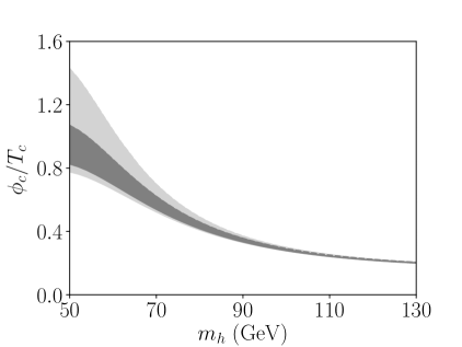
Figure 5: Left: $T_{\rm c}$ in a toy SM as a function of a light Higgs mass, in Landau gauge. Bands illustrate intrinsic uncertainty related to varying 4d RG scale in $\mu=(0.5\dots 2.0)\times\pi T$, with two- (dark grey) and one-loop (light grey) thermal mass. Right: As left panel but for $\phi_{{\mbox{\scriptsize c}}}/T_{\rm c}$.

The leftover 4d scale dependence is illustrated by the resulting bands from varying $\mu=(0.5\dots 2.0)\times\pi T$ and by showing the result with the two-loop (one-loop) thermal mass in dark grey (light grey). A larger band in the latter case signals a larger intrinsic uncertainty, and reinforces our key message of the importance of the two-loop thermal mass. In BSM theories that involve large portal couplings to the Higgs, this theoretical uncertainty related to a leftover scale dependency can be even worse. In the SM, the top quark contributions dominate over those related to gauge couplings and the Higgs self-interaction. We note, that the running of the top quark contribution in the one-loop thermal mass that causes the dominant effect on the broader band, is exactly the same contribution that causes a similar uncertainty for a SMEFT study [63], since this model has exactly the same one-loop thermal mass. The dominant uncertainty in SMEFT roots in the SM sector and is not related to the new higher dimensional sextic Higgs operator.

From fig. 5 (right), we observe that the transition strength increases for lower Higgs mass which corresponds to smaller Higgs self-coupling and a smaller dimensionless 3d quantity $x\equiv\lambda_{h,3}/g^{2}_{3}$. This quantity $x$ is the expansion parameter of 3d perturbation theory [60, 59]. The smaller it is, the better 3d perturbation theory works. However, for smaller $x$ the 3d matching relations are also relatively more sensitive to the 4d renormalisation scale, and in the end the total uncertainty is larger. This provides a counter-example for the common folklore which states that strong phase transitions (with large $\phi_{{\mbox{\scriptsize c}}}/T_{\rm c}$) are better described in perturbation theory, than weak transitions. On the other hand, fig. 5 makes it evident that perturbation theory is oblivious to the crossover character of the SM phase transition after an end-point around $m_{h}\sim 70$ GeV [7]. There is still a discontinuity in critical value $\phi_{{\mbox{\scriptsize c}}}$ (indicated by its non-zero value). In fact, perturbation theory predicts a first-order phase transition and fails even at a qualitative level. This showcases the theoretical challenge to describe phase transition thermodynamics.

References

- [1] M. J. Ramsey-Musolf, The electroweak phase transition: a collider target, JHEP 09 (2020) 179 [1912.07189].
- [2] A. Papaefstathiou and G. White, The electro-weak phase transition at colliders: confronting theoretical uncertainties and complementary channels, JHEP 05 (2021) 099 [2010.00597].
- [3] M. Chala, M. Ramos, and M. Spannowsky, Gravitational wave and collider probes of a triplet Higgs sector with a low cutoff, Eur. Phys. J. C 79 (2019) 156 [1812.01901].
- [4] C. Caprini et al., Detecting gravitational waves from cosmological phase transitions with LISA: an update, JCAP 03 (2020) 024 [1910.13125].
- [5] D. E. Morrissey and M. J. Ramsey-Musolf, Electroweak baryogenesis, New J. Phys. 14 (2012) 125003 [1206.2942].
- [6] G. A. White, A Pedagogical Introduction to Electroweak Baryogenesis. 2053-2571. Morgan & Claypool Publishers, 2016.
- [7] K. Kajantie, M. Laine, K. Rummukainen, and M. E. Shaposhnikov, The Electroweak phase transition: A Nonperturbative analysis, Nucl. Phys. B 466 (1996) 189 [hep-lat/9510020].
- [8] K. Kajantie, M. Laine, K. Rummukainen, and M. E. Shaposhnikov, Is there a hot electroweak phase transition at m(H) larger or equal to m(W)?, Phys. Rev. Lett. 77 (1996) 2887 [hep-ph/9605288].
- [9] K. Kajantie, M. Laine, K. Rummukainen, and M. E. Shaposhnikov, A Nonperturbative analysis of the finite T phase transition in electroweak theory, Nucl. Phys. B 493 (1997) 413 [hep-lat/9612006].
- [10] F. Csikor, Z. Fodor, and J. Heitger, Endpoint of the hot electroweak phase transition, Phys. Rev. Lett. 82 (1999) 21 [hep-ph/9809291].
- [11] M. D’Onofrio and K. Rummukainen, Standard model cross-over on the lattice, Phys. Rev. D 93 (2016) 025003 [1508.07161].
- [12] M. Pietroni, The Electroweak phase transition in a nonminimal supersymmetric model, Nucl. Phys. B 402 (1993) 27 [hep-ph/9207227].
- [13] J. M. Cline and P.-A. Lemieux, Electroweak phase transition in two Higgs doublet models, Phys. Rev. D 55 (1997) 3873 [hep-ph/9609240].
- [14] S. W. Ham, S. K. OH, C. M. Kim, E. J. Yoo, and D. Son, Electroweak phase transition in a nonminimal supersymmetric model, Phys. Rev. D 70 (2004) 075001 [hep-ph/0406062].
- [15] K. Funakubo, S. Tao, and F. Toyoda, Phase transitions in the NMSSM, Prog. Theor. Phys. 114 (2005) 369 [hep-ph/0501052].
- [16] V. Barger, P. Langacker, M. McCaskey, M. Ramsey-Musolf, and G. Shaughnessy, Complex Singlet Extension of the Standard Model, Phys. Rev. D 79 (2009) 015018 [0811.0393].
- [17] D. J. H. Chung and A. J. Long, Electroweak Phase Transition in the munuSSM, Phys. Rev. D 81 (2010) 123531 [1004.0942].
- [18] J. R. Espinosa, T. Konstandin, and F. Riva, Strong Electroweak Phase Transitions in the Standard Model with a Singlet, Nucl. Phys. B 854 (2012) 592 [1107.5441].
- [19] T. A. Chowdhury, M. Nemevsek, G. Senjanovic, and Y. Zhang, Dark Matter as the Trigger of Strong Electroweak Phase Transition, JCAP 02 (2012) 029 [1110.5334].
- [20] G. Gil, P. Chankowski, and M. Krawczyk, Inert Dark Matter and Strong Electroweak Phase Transition, Phys. Lett. B 717 (2012) 396 [1207.0084].
- [21] M. Carena, G. Nardini, M. Quiros, and C. E. Wagner, MSSM Electroweak Baryogenesis and LHC Data, JHEP 02 (2013) 001 [1207.6330].
- [22] J. M. No and M. Ramsey-Musolf, Probing the Higgs Portal at the LHC Through Resonant di-Higgs Production, Phys. Rev. D 89 (2014) 095031 [1310.6035].
- [23] G. C. Dorsch, S. J. Huber, and J. M. No, A strong electroweak phase transition in the 2HDM after LHC8, JHEP 10 (2013) 029 [1305.6610].
- [24] D. Curtin, P. Meade, and C.-T. Yu, Testing Electroweak Baryogenesis with Future Colliders, JHEP 11 (2014) 127 [1409.0005].
- [25] W. Huang, Z. Kang, J. Shu, P. Wu, and J. M. Yang, New insights in the electroweak phase transition in the NMSSM, Phys. Rev. D 91 (2015) 025006 [1405.1152].
- [26] S. Profumo, M. J. Ramsey-Musolf, C. L. Wainwright, and P. Winslow, Singlet-catalyzed electroweak phase transitions and precision Higgs boson studies, Phys. Rev. D 91 (2015) 035018 [1407.5342].
- [27] J. Kozaczuk, S. Profumo, L. S. Haskins, and C. L. Wainwright, Cosmological Phase Transitions and their Properties in the NMSSM, JHEP 01 (2015) 144 [1407.4134].
- [28] M. Jiang, L. Bian, W. Huang, and J. Shu, Impact of a complex singlet: Electroweak baryogenesis and dark matter, Phys. Rev. D 93 (2016) 065032 [1502.07574].
- [29] D. Curtin, P. Meade, and H. Ramani, Thermal Resummation and Phase Transitions, Eur. Phys. J. C 78 (2018) 787 [1612.00466].
- [30] V. Vaskonen, Electroweak baryogenesis and gravitational waves from a real scalar singlet, Phys. Rev. D 95 (2017) 123515 [1611.02073].
- [31] G. Dorsch, S. Huber, T. Konstandin, and J. No, A Second Higgs Doublet in the Early Universe: Baryogenesis and Gravitational Waves, JCAP 05 (2017) 052 [1611.05874].
- [32] P. Huang, A. J. Long, and L.-T. Wang, Probing the Electroweak Phase Transition with Higgs Factories and Gravitational Waves, Phys. Rev. D 94 (2016) 075008 [1608.06619].
- [33] M. Chala, G. Nardini, and I. Sobolev, Unified explanation for dark matter and electroweak baryogenesis with direct detection and gravitational wave signatures, Phys. Rev. D 94 (2016) 055006 [1605.08663].
- [34] P. Basler, M. Krause, M. Muhlleitner, J. Wittbrodt, and A. Wlotzka, Strong First Order Electroweak Phase Transition in the CP-Conserving 2HDM Revisited, JHEP 02 (2017) 121 [1612.04086].
- [35] A. Beniwal, M. Lewicki, J. D. Wells, M. White, and A. G. Williams, Gravitational wave, collider and dark matter signals from a scalar singlet electroweak baryogenesis, JHEP 08 (2017) 108 [1702.06124].
- [36] J. Bernon, L. Bian, and Y. Jiang, A new insight into the phase transition in the early Universe with two Higgs doublets, JHEP 05 (2018) 151 [1712.08430].
- [37] G. Kurup and M. Perelstein, Dynamics of Electroweak Phase Transition In Singlet-Scalar Extension of the Standard Model, Phys. Rev. D 96 (2017) 015036 [1704.03381].
- [38] J. O. Andersen, T. Gorda, A. Helset, et al., Nonperturbative Analysis of the Electroweak Phase Transition in the Two Higgs Doublet Model, Phys. Rev. Lett. 121 (2018) 191802 [1711.09849].
- [39] C.-W. Chiang, M. J. Ramsey-Musolf, and E. Senaha, Standard Model with a Complex Scalar Singlet: Cosmological Implications and Theoretical Considerations, Phys. Rev. D 97 (2018) 015005 [1707.09960].
- [40] G. C. Dorsch, S. J. Huber, K. Mimasu, and J. M. No, The Higgs Vacuum Uplifted: Revisiting the Electroweak Phase Transition with a Second Higgs Doublet, JHEP 12 (2017) 086 [1705.09186].
- [41] A. Beniwal, M. Lewicki, M. White, and A. G. Williams, Gravitational waves and electroweak baryogenesis in a global study of the extended scalar singlet model, JHEP 02 (2019) 183 [1810.02380].
- [42] S. Bruggisser, B. Von Harling, O. Matsedonskyi, and G. Servant, Electroweak Phase Transition and Baryogenesis in Composite Higgs Models, JHEP 12 (2018) 099 [1804.07314].
- [43] P. Athron, C. Balazs, A. Fowlie, G. Pozzo, G. White, and Y. Zhang, Strong first-order phase transitions in the NMSSM — a comprehensive survey, JHEP 11 (2019) 151 [1908.11847].
- [44] K. Kainulainen, V. Keus, L. Niemi, K. Rummukainen, T. V. I. Tenkanen, and V. Vaskonen, On the validity of perturbative studies of the electroweak phase transition in the Two Higgs Doublet model, JHEP 06 (2019) 075 [1904.01329].
- [45] L. Bian, Y. Wu, and K.-P. Xie, Electroweak phase transition with composite Higgs models: calculability, gravitational waves and collider searches, JHEP 12 (2019) 028 [1909.02014].
- [46] H.-L. Li, M. Ramsey-Musolf, and S. Willocq, Probing a scalar singlet-catalyzed electroweak phase transition with resonant di-Higgs boson production in the channel, Phys. Rev. D 100 (2019) 075035 [1906.05289].
- [47] C.-W. Chiang and B.-Q. Lu, First-order electroweak phase transition in a complex singlet model with symmetry, JHEP 07 (2020) 082 [1912.12634].
- [48] K.-P. Xie, Y. Wu, and L. Bian, Electroweak baryogenesis and gravitational waves in a composite Higgs model with high dimensional fermion representations, [2005.13552].
- [49] N. F. Bell, M. J. Dolan, L. S. Friedrich, M. J. Ramsey-Musolf, and R. R. Volkas, Two-Step Electroweak Symmetry-Breaking: Theory Meets Experiment, JHEP 05 (2020) 050 [2001.05335].
- [50] C. P. Burgess, M. Pospelov, and T. ter Veldhuis, The Minimal model of nonbaryonic dark matter: A Singlet scalar, Nucl. Phys. B 619 (2001) 709 [hep-ph/0011335].
- [51] M. Gonderinger, H. Lim, and M. J. Ramsey-Musolf, Complex Scalar Singlet Dark Matter: Vacuum Stability and Phenomenology, Phys. Rev. D 86 (2012) 043511 [1202.1316].
- [52] W. Chao, First order electroweak phase transition triggered by the Higgs portal vector dark matter, Phys. Rev. D 92 (2015) 015025 [1412.3823].
- [53] A. D. Linde, Infrared Problem in Thermodynamics of the Yang-Mills Gas, Phys. Lett. B 96 (1980) 289.
- [54] P. B. Arnold, Phase transition temperatures at next-to-leading order, Phys. Rev. D 46 (1992) 2628 [hep-ph/9204228].
- [55] P. H. Ginsparg, First Order and Second Order Phase Transitions in Gauge Theories at Finite Temperature, Nucl. Phys. B170 (1980) 388.
- [56] T. Appelquist and R. D. Pisarski, High-Temperature Yang-Mills Theories and Three-Dimensional Quantum Chromodynamics, Phys. Rev. D23 (1981) 2305.
- [57] E. Braaten and A. Nieto, Effective field theory approach to high temperature thermodynamics, Phys. Rev. D51 (1995) 6990 [hep-ph/9501375].
- [58] K. Kajantie, M. Laine, K. Rummukainen, and M. E. Shaposhnikov, Generic rules for high temperature dimensional reduction and their application to the standard model, Nucl. Phys. B 458 (1996) 90 [hep-ph/9508379].
- [59] K. Farakos, K. Kajantie, K. Rummukainen, and M. E. Shaposhnikov, 3d physics and the electroweak phase transition: A Framework for lattice Monte Carlo analysis, Nucl. Phys. B442 (1995) 317 [hep-lat/9412091].
- [60] K. Farakos, K. Kajantie, K. Rummukainen, and M. E. Shaposhnikov, 3-D physics and the electroweak phase transition: Perturbation theory, Nucl. Phys. B 425 (1994) 67 [hep-ph/9404201].
- [61] P. B. Arnold and O. Espinosa, The Effective potential and first order phase transitions: Beyond leading-order, Phys. Rev. D 47 (1993) 3546 [hep-ph/9212235].
- [62] O. Gould and T. V. I. Tenkanen, On the perturbative expansion at high temperature and implications for cosmological phase transitions, [2104.04399].
- [63] D. Croon, O. Gould, P. Schicho, T. V. I. Tenkanen, and G. White, Theoretical uncertainties for cosmological first-order phase transitions, JHEP 04 (2021) 055 [2009.10080].
- [64] L. Niemi, P. Schicho, and T. V. I. Tenkanen, Singlet-assisted electroweak phase transition at two loops, Phys. Rev. D 103 (2021) 115035 [2103.07467].
- [65] H. H. Patel and M. J. Ramsey-Musolf, Baryon Washout, Electroweak Phase Transition, and Perturbation Theory, JHEP 07 (2011) 029 [1101.4665].
- [66] M. Laine, Gauge dependence of the high temperature two loop effective potential for the Higgs field, Phys. Rev. D 51 (1995) 4525 [hep-ph/9411252].
- [67] N. K. Nielsen, On the Gauge Dependence of Spontaneous Symmetry Breaking in Gauge Theories, Nucl. Phys. B 101 (1975) 173.
- [68] R. Fukuda and T. Kugo, Gauge Invariance in the Effective Action and Potential, Phys. Rev. D 13 (1976) 3469.
- [69] L. Niemi, M. J. Ramsey-Musolf, T. V. I. Tenkanen, and D. J. Weir, Thermodynamics of a Two-Step Electroweak Phase Transition, Phys. Rev. Lett. 126 (2021) 171802 [2005.11332].
- [70] M. Laine and M. Meyer, Standard Model thermodynamics across the electroweak crossover, JCAP 07 (2015) 035 [1503.04935].
- [71] A. Ekstedt and J. Löfgren, A Critical Look at the Electroweak Phase Transition, JHEP 12 (2020) 136 [2006.12614].
- [72] O. Gould and J. Hirvonen, Effective field theory approach to thermal bubble nucleation, Phys. Rev. D 104 (2021) 096015 [2108.04377].
- [73] J. Hirvonen, J. Löfgren, M. J. Ramsey-Musolf, P. Schicho, and T. V. I. Tenkanen, Computing the gauge-invariant bubble nucleation rate in finite temperature effective field theory, [2112.08912].
- [74] A. Ekstedt, Higher-order corrections to the bubble-nucleation rate at finite temperature, Eur. Phys. J. C 82 (2022) 173 [2104.11804].
- [75] A. Ekstedt, Bubble Nucleation to All Orders, [2201.07331].
- [76] M. Garny and T. Konstandin, On the gauge dependence of vacuum transitions at finite temperature, JHEP 07 (2012) 189 [1205.3392].
- [77] J. Löfgren, M. J. Ramsey-Musolf, P. Schicho, and T. V. I. Tenkanen, Nucleation at finite temperature: a gauge-invariant, perturbative framework, [2112.05472].
- [78] R. R. Parwani, Resummation in a hot scalar field theory, Phys. Rev. D 45 (1992) 4695 [hep-ph/9204216].
- [79] N. Chen, T. Li, Y. Wu, and L. Bian, Complementarity of the future colliders and gravitational waves in the probe of complex singlet extension to the standard model, Phys. Rev. D 101 (2020) 075047 [1911.05579].
- [80] G.-C. Cho, C. Idegawa, and E. Senaha, Electroweak phase transition in a complex singlet extension of the Standard Model with degenerate scalars, Phys. Lett. B 823 (2021) 136787 [2105.11830].
- [81] P. M. Schicho, T. V. I. Tenkanen, and J. Österman, Robust approach to thermal resummation: Standard Model meets a singlet, JHEP 06 (2021) 130 [2102.11145].
- [82] A. Ekstedt, O. Gould, and J. Löfgren, Radiative first-order phase transitions to next-to-next-to-leading-order, forthcoming (2022) .
- [83] O. Gould and T. V. I. Tenkanen, Two-step electroweak phase transition in perturbation theory, forthcoming (2022) .
- [84] C. L. Wainwright, CosmoTransitions: Computing Cosmological Phase Transition Temperatures and Bubble Profiles with Multiple Fields, Comput. Phys. Commun. 183 (2012) 2006 [1109.4189].
- [85] P. Basler and M. Mühlleitner, BSMPT (Beyond the Standard Model Phase Transitions): A tool for the electroweak phase transition in extended Higgs sectors, Comput. Phys. Commun. 237 (2019) 62 [1803.02846].
- [86] P. Basler, M. Mühlleitner, and J. Müller, BSMPT v2 a tool for the electroweak phase transition and the baryon asymmetry of the universe in extended Higgs Sectors, Comput. Phys. Commun. 269 (2021) 108124 [2007.01725].
- [87] P. Athron, C. Balázs, A. Fowlie, and Y. Zhang, PhaseTracer: tracing cosmological phases and calculating transition properties, Eur. Phys. J. C 80 (2020) 567 [2003.02859].
- [88] T. Brauner, T. V. I. Tenkanen, A. Tranberg, A. Vuorinen, and D. J. Weir, Dimensional reduction of the Standard Model coupled to a new singlet scalar field, JHEP 03 (2017) 007 [1609.06230].
- [89] O. Gould, Real scalar phase transitions: a nonperturbative analysis, JHEP 04 (2021) 057 [2101.05528].
- [90] A. Jakovac, K. Kajantie, and A. Patkos, A Hierarchy of effective field theories of hot electroweak matter, Phys. Rev. D 49 (1994) 6810 [hep-ph/9312355].
- [91] A. Ekstedt, P. Schicho, and T. V. I. Tenkanen, DRalgo: package for dimensional reduction and two-loop thermal effective potential in hot electroweak theories, forthcoming (2022) .
- [92] M. Laine, Exact relation of lattice and continuum parameters in three-dimensional SU(2) + Higgs theories, Nucl. Phys. B 451 (1995) 484 [hep-lat/9504001].
- [93] M. Laine and A. Rajantie, Lattice-continuum relations for 3d SU(N) + Higgs theories, Nucl. Phys. B 513 (1998) 471 [hep-lat/9705003].
- [94] K. Kajantie, M. Laine, K. Rummukainen, and Y. Schroder, The Pressure of hot QCD up to g6 ln(1/g), Phys. Rev. D 67 (2003) 105008 [hep-ph/0211321].
- [95] K. Kajantie, M. Laine, K. Rummukainen, and Y. Schroder, Four loop vacuum energy density of the SU(N(c)) + adjoint Higgs theory, JHEP 04 (2003) 036 [hep-ph/0304048].
- [96] A. Gynther and M. Vepsäläinen, Pressure of the standard model near the electroweak phase transition, JHEP 03 (2006) 011 [hep-ph/0512177].
- [97] A. Gynther and M. Vepsäläinen, Pressure of the standard model at high temperatures, JHEP 01 (2006) 060 [hep-ph/0510375].
- [98] A. K. Rajantie, Feynman diagrams to three loops in three-dimensional field theory, Nucl. Phys. B 480 (1996) 729 [hep-ph/9606216].
- [99] C. Delaunay, C. Grojean, and J. D. Wells, Dynamics of Non-renormalizable Electroweak Symmetry Breaking, JHEP 04 (2008) 029 [0711.2511].
- [100] J. R. Espinosa and M. Quiros, Novel Effects in Electroweak Breaking from a Hidden Sector, Phys. Rev. D 76 (2007) 076004 [hep-ph/0701145].
- [101] S. Profumo, M. J. Ramsey-Musolf, and G. Shaughnessy, Singlet Higgs phenomenology and the electroweak phase transition, JHEP 08 (2007) 010 [0705.2425].
- [102] A. Noble and M. Perelstein, Higgs self-coupling as a probe of electroweak phase transition, Phys. Rev. D 78 (2008) 063518 [0711.3018].
- [103] J. R. Espinosa, T. Konstandin, J. M. No, and M. Quiros, Some Cosmological Implications of Hidden Sectors, Phys. Rev. D 78 (2008) 123528 [0809.3215].
- [104] N. Blinov, J. Kozaczuk, D. E. Morrissey, and C. Tamarit, Electroweak Baryogenesis from Exotic Electroweak Symmetry Breaking, Phys. Rev. D 92 (2015) 035012 [1504.05195].
- [105] P. Basler, M. Mühlleitner, and J. Wittbrodt, The CP-Violating 2HDM in Light of a Strong First Order Electroweak Phase Transition and Implications for Higgs Pair Production, JHEP 03 (2018) 061 [1711.04097].
- [106] M. Chala, C. Krause, and G. Nardini, Signals of the electroweak phase transition at colliders and gravitational wave observatories, JHEP 07 (2018) 062 [1802.02168].
- [107] M. Carena, Z. Liu, and Y. Wang, Electroweak phase transition with spontaneous Z2-breaking, JHEP 08 (2020) 107 [1911.10206].
- [108] T. Gorda, A. Helset, L. Niemi, T. V. I. Tenkanen, and D. J. Weir, Three-dimensional effective theories for the two Higgs doublet model at high temperature, JHEP 02 (2019) 081 [1802.05056].
- [109] L. Niemi, H. H. Patel, M. J. Ramsey-Musolf, T. V. I. Tenkanen, and D. J. Weir, Electroweak phase transition in the real triplet extension of the SM: Dimensional reduction, Phys. Rev. D 100 (2019) 035002 [1802.10500].
- [110] H. H. Patel, M. J. Ramsey-Musolf, and M. B. Wise, Color Breaking in the Early Universe, Phys. Rev. D 88 (2013) 015003 [1303.1140].
- [111] S. Inoue, G. Ovanesyan, and M. J. Ramsey-Musolf, Two-Step Electroweak Baryogenesis, Phys. Rev. D 93 (2016) 015013 [1508.05404].
- [112] D. Bodeker, P. John, M. Laine, and M. G. Schmidt, The Two loop MSSM finite temperature effective potential with stop condensation, Nucl. Phys. B 497 (1997) 387 [hep-ph/9612364].
- [113] M. Laine, M. Meyer, and G. Nardini, Thermal phase transition with full 2-loop effective potential, Nucl. Phys. B 920 (2017) 565 [1702.07479].
- [114] A. Papaefstathiou and G. White, The Electro-Weak Phase Transition at Colliders: Discovery Post-Mortem, JHEP 02 (2022) 185 [2108.11394].
- [115] J. Kripfganz, A. Laser, and M. G. Schmidt, The high-temperature two-loop effective potential of the electroweak theory in a general ’t Hooft background gauge, Phys. Lett. B 351 (1995) 266 [9501317].
- [116] D. Croon, R. Houtz, and V. Sanz, Dynamical Axions and Gravitational Waves, JHEP 07 (2019) 146 [1904.10967].
- [117] C. G. Boyd, D. E. Brahm, and S. D. H. Hsu, Resummation methods at finite temperature: The Tadpole way, Phys. Rev. D 48 (1993) 4963 [hep-ph/9304254].
- [118] M. Laine and M. Losada, Two loop dimensional reduction and effective potential without temperature expansions, Nucl. Phys. B 582 (2000) 277 [hep-ph/0003111].
- [119] Particle Data Group Collaboration, M. Tanabashi et al., Review of Particle Physics, Phys. Rev. D 98 (2018) 030001.
- [120] A. J. Andreassen, Gauge Dependence of the Quantum Field Theory Effective Potential, Master’s thesis, Norwegian U. Sci. Tech., 2013.