Extrapolated Proportional-Integral Projected Gradient Method for Conic Optimization

Abstract

Conic optimization is the minimization of a convex quadratic function subject to conic constraints. We introduce a novel first-order method for conic optimization, named extrapolated proportional-integral projected gradient method (xPIPG), that automatically detects infeasibility. The iterates of xPIPG either asymptotically satisfy a set of primal-dual optimality conditions, or generate a proof of primal or dual infeasibility. We demonstrate the application of xPIPG using benchmark problems in model predictive control. xPIPG outperforms many state-of-the-art conic optimization solvers, especially when solving large-scale problems.

Optimization algorithms, infeasibility detection

1 Introduction

Conic optimization is the minimization of a quadratic function subject to conic constraints:

$$\begin{array}[]{ll}\underset{z}{\mbox{minimize}}&\frac{1}{2}z^{\top}Pz+q^{\top}z\\ \mbox{subject to}&Hz-g\in\mathbb{K},\enskip z\in\mathbb{D},\end{array}$$ (1)

where $P\in\mathbb{R}^{n\times n}$ is a symmetric positive semidefinite matrix, $H\in\mathbb{R}^{m\times n}$, $g\in\mathbb{R}^{m}$, $\mathbb{K}\subset\mathbb{R}^{m}$ is a closed convex cone, and $\mathbb{D}\subset\mathbb{R}^{n}$ is a closed convex set.

An important subproblem in conic optimization is to detect whether optimization (1) is primal or dual infeasible [1, 2, 3, 4, 5, 6]. Optimization (1) is primal infeasible if there exists $\overline{w}\in\mathbb{R}^{m}$ such that

$$\underset{z\in\mathbb{D}}{\inf}\,\langle Hz-g,\overline{w}\rangle>\underset{y\in\mathbb{K}}{\sup}\,\langle y,\overline{w}\rangle.$$ (2)

Here the vector $\overline{w}$ is known as a proof of primal infeasibility; it defines a hyperplane separating the set $\{Hz-g\,|\,z\in\mathbb{D}\}$ from the cone $\mathbb{K}$. On the other hand, optimization (1) is dual infeasible if there exists $\overline{z}\in\mathbb{R}^{n}$ such that the following conditions hold for all $z\in\mathbb{D}$:

$$P\overline{z}=0,\enskip q^{\top}\overline{z}<0,\enskip H\overline{z}\in\mathbb{K},\enskip z+\overline{z}\in\mathbb{D}.$$ (3)

Here the vector $\overline{z}$ is known as a proof of dual infeasibility; it defines a direction along which the value of the objective function of optimization (1) can decrease indefinitely. We refer the interested readers to [2, Prop. 3.1] and [7, Prop. 4.1] for details on the infeasibility conditions in (2) and (3). Infeasibility detection is the problem of computing, if possible, a proof of primal infeasibility or dual infeasibility [2, 3, 5]. Such computation is necessary in both quasiconvex and mixed-integer optimization [5].

Traditional conic optimization methods detect infeasibility by computing matrix inverse (or equivalently, solving system of linear equations), usually as a subroutine of the interior-point method [8] or the Douglas-Rachford-splitting method [9, 1, 10, 11, 2, 4]. Such computation is numerically expensive for large-scale problems.

Proportional-integral projected gradient method (PIPG) is the first method that detects infeasibility in general conic optimization without solving systems of linear equations [5]. If the conic optimization is feasible, PIPG also enjoys the best convergence rates among first-order primal-dual methods. For a detailed comparison between PIPG and other first-order methods, see [12, 13, 14].

By adding an extrapolation step to PIPG, we introduce a novel conic optimization method, named extrapolated PIPG (xPIPG), that automatically detects infeasibility. Previous results only showed the ergodic convergence of the primal-dual gap function for a variant of xPIPG [12]. We prove that the iterates of xPIPG either asymptotically satisfy a set of primal-dual optimality conditions, or generates a proof of primal or dual infeasibility.

We demonstrate the application of xPIPG using the optimal control problem of oscillating masses, a popular benchmark problem in model predictive control [15, 16, 14]. Empirically, xPIPG is about twice as fast as PIPG. With an efficient implementation in C language, xPIPG outperforms many state-of-the-art solvers, especially when solving large-scale problems.

2 Notation and preliminaries

We let $\mathbb{N}$, $\mathbb{R}$ and $\mathbb{R}_{+}$ denote the set of positive integers, real numbers, and non-negative real numbers, respectively. For two vectors $z,z^{\prime}\in\mathbb{R}^{n}$ and a positive definite matrix $M$, we let $\langle z,z^{\prime}\rangle$ denote the inner product of $z$ and $z^{\prime}$, and $\langle z,z^{\prime}\rangle_{M}$ denote the inner product of $z$ and $z^{\prime}$ weighted by matrix $M$; we let $\left\lVert z\right\rVert\coloneqq\sqrt{\langle z,z\rangle}$ denote the $\ell_{2}$-norm of $z$, and $\left\lVert z\right\rVert_{M}\coloneqq\sqrt{\langle z,Mz\rangle}$ denote the norm of $z$ weighted by matrix $M$. We let $1_{n}$ denote the $n$-dimensional vector of all 1’s, $0_{n}$ denote the $n$-dimensional zero vector, and $I_{n}$ denote the $n\times n$ identity matrix. For a matrix $H\in\mathbb{R}^{m\times n}$, we let $H^{\top}$ denote its transpose, $\left\lVert H\right\rVert$ denote its largest singular value. A set $\mathbb{D}\subseteq\mathbb{R}^{n}$ is convex if $\alpha z+(1-\alpha)z^{\prime}\in\mathbb{D}$ for any $\alpha\in[0,1]$ and $z,z^{\prime}\in\mathbb{D}$. A set $\mathbb{K}\subseteq\mathbb{R}^{m}$ is a convex cone if $\mathbb{K}$ is convex and $\alpha w\in\mathbb{K}$ for any $w\in\mathbb{K}$ and $\alpha\in\mathbb{R}_{+}$.

Let $\mathbb{D}\subseteq\mathbb{R}^{n}$ be a nonempty closed convex set. The point-to-set distance from $z\in\mathbb{R}^{n}$ to set $\mathbb{D}$ is given by

$$d(z\,|\,\mathbb{D})\coloneqq\underset{z^{\prime}\in\mathbb{D}}{\min}\left\lVert z-z^{\prime}\right\rVert.$$ (4)

The projection of $z$ onto set $\mathbb{D}$ is given by

$$\pi_{\mathbb{D}}[z]\coloneqq\underset{z^{\prime}\in\mathbb{D}}{\mathop{\rm argmin}}\left\lVert z-z^{\prime}\right\rVert.$$ (5)

The normal cone of set $\mathbb{D}$ at $z$ is given by

$$N_{\mathbb{D}}(z)\coloneqq\{y\in\mathbb{R}^{n}\,|\,\langle y,z^{\prime}-z\rangle\leq 0,\forall z^{\prime}\in\mathbb{D}\}.$$ (6)

The recession cone of set $\mathbb{D}$ is a given by

$$\mathrm{rec\,}\mathbb{D}\coloneqq\{y\in\mathbb{R}^{n}\,|\,y+z\in\mathbb{D},\forall\,z\in\mathbb{D}\}.$$ (7)

The support function of set $\mathbb{D}$ is given by

$$\sigma_{\mathbb{D}}(z)\coloneqq\sup_{y\in\mathbb{D}}\,\langle y,z\rangle$$ (8)

for all $z\in\mathbb{R}^{n}$. Let $\mathbb{K}\subseteq\mathbb{R}^{m}$ be a nonempty closed convex cone. The recession cone of cone $\mathbb{K}$ is itself, i.e., $\mathrm{rec\,}\mathbb{K}=\mathbb{K}$ [17, Cor. 6.50]. The polar cone of $\mathbb{K}$ is given by

$$\mathbb{K}^{\circ}\coloneqq\{w\in\mathbb{R}^{m}\,|\,\langle w,y\rangle\leq 0,\forall\,y\in\mathbb{K}\}.$$ (9)

Let $M\in\mathbb{R}^{p\times p}$ be a symmetric positive definite matrix. A function $T:\mathbb{R}^{p}\to\mathbb{R}^{p}$ is a $\gamma$-averaged operator for some $\gamma\in(0,1)$ with respect to norm $\left\lVert\cdot\right\rVert_{M}$ if and only if the following condition holds for any $\zeta_{1},\zeta_{2}\in\mathbb{R}^{p}$ [17, Prop. 4.35]:

$$\left\lVert T(\zeta_{1})-T(\zeta_{2})\right\rVert_{M}^{2}-\left\lVert\zeta_{1}-\zeta_{2}\right\rVert_{M}^{2}$$ (10)

$$\textstyle\leq\frac{\gamma-1}{\gamma}\left\lVert\zeta_{1}-\zeta_{2}-T(\zeta_{1})+T(\zeta_{2})\right\rVert_{M}^{2}.$$

We will use the following results on averaged operators.

Lemma 1.

[2, Lem. 5.1] Let $M\in\mathbb{R}^{p\times p}$ be a symmetric positive definite matrix and $T:\mathbb{R}^{p}\to\mathbb{R}^{p}$ be a $\gamma$-averaged operator for some $\gamma\in(0,1)$ with respect to norm $\left\lVert\cdot\right\rVert_{M}$. Let $\zeta^{1}\in\mathbb{R}^{p}$ and $\zeta^{j+1}\coloneqq T(\zeta^{j})$ for all $j\in\mathbb{N}$. Then there exists $\overline{\zeta}\in\mathbb{R}^{p}$, known as the minimal-displacement vector of operator $T$, such that $\textstyle\lim\limits_{j\to\infty}\frac{\zeta^{j}}{j}=\lim\limits_{j\to\infty}\zeta^{j+1}-\zeta^{j}=\overline{\zeta}$.

3 Extrapolated proportional-integral projected gradient method

We introduce our main contribution, a conic optimization method that automatically detects infeasibility, in Algorithm 1, where $\alpha,\beta,\rho\in\mathbb{R}_{+}$ are positive step sizes, $k\in\mathbb{N}$ is the maximum number of iterations, $\epsilon\in\mathbb{R}_{+}$ is a small tolerance for infeasibility.

We name Algorithm 1 the extrapolated proportional-integral projected gradient method for the following reasons. First, if $\rho=1$, then Algorithm 1 reduces to the proportional-integral projected gradient method (PIPG) [12, 13, 14], which has been used in distributed optimization [18, 19] and optimal control [13, 20]. Second, lines 5–6 define an interpolation step if $\rho\in[0,1]$ and an extrapolation step if $\rho\in[1,2]$; see Fig. 1 for an illustration. Since extrapolation improves practical convergence [21, 12], we will let $\rho\in[1,2]$ in Algorithm 1, hence the name “extrapolated PIPG”.

Algorithm 1 xPIPG

1:$k,\alpha,\beta,\rho,\epsilon$, initial values $\xi^{1},\eta^{1}$.

2:for $j=1,2,\ldots,k$ do

3:     $z^{j+1}=\pi_{\mathbb{D}}[\xi^{j}-\alpha(P\xi^{j}+q+H^{\top}\eta^{j})]$

4:     $w^{j+1}=\pi_{\mathbb{K}^{\circ}}[\eta^{j}+\beta(H(2z^{j+1}-\xi^{j})-g)]$

5:     $\xi^{j+1}=(1-\rho)\xi^{j}+\rho z^{j+1}$

6:     $\eta^{j+1}=(1-\rho)\eta^{j}+\rho w^{j+1}$

7:end for

8:if $\max\{\frac{1}{\alpha\rho}\left\lVert z^{k+1}-z^{k}\right\rVert,\frac{1}{\beta\rho}\left\lVert w^{k+1}-w^{k}\right\rVert\}\leq\epsilon$ then

9:     return $z^{k}$

10:else

11:     if $\frac{1}{\beta\rho}\left\lVert w^{k+1}-w^{k}\right\rVert>\epsilon$ then

12:         return “Primal infeasible”

13:     end if

14:     if $\frac{1}{\alpha\rho}\left\lVert z^{k+1}-z^{k}\right\rVert>\epsilon$ then

15:         return “Dual infeasible”

16:     end if

17:end if

Figure 1: The range of $\xi^{j+1}$ in Algorithm 1.

Previous results already showed that the iterations in Algorithm 1 ensure that, along certain averaged sequence of iterates, the primal-dual gap function converges to zero at the rate of $O(1/k)$ [12, Thm. 2]. We will further show that for using a large enough iteration number $k$ and a small enough tolerance $\epsilon$, Algorithm 1 automatically detects the primal and dual infeasibility of optimization (1), just like its special case where $\rho=1$ [14, Thm. 1].

We start with the following assumptions.

Assumption 1.

Matrix $P\in\mathbb{R}^{n\times n}$ is symmetric and positive semidefinite, set $\mathbb{D}\subset\mathbb{R}^{n}$ is closed and convex, cone $\mathbb{K}\subset\mathbb{R}^{m}$ is closed and convex.

With these assumptions, the following lemma shows that line 3 to line 6 in Algorithm 1 are equivalent to the fixed-point iteration of an averaged operator.

Lemma 2.

Suppose that Assumption 1 holds. Let $\zeta^{j}=\begin{bmatrix}(\xi^{j})^{\top}&(\eta^{j})^{\top}\end{bmatrix}^{\top}$ for all $j=1,2,\ldots,k$ in Algorithm 1 and $M=\begin{bmatrix}\frac{1}{\alpha}I-P&-H^{\top}\\ -H&\frac{1}{\beta}I\end{bmatrix}$. If $\alpha,\beta>0$, $\alpha(\left\lVert P\right\rVert+\beta\left\lVert H\right\rVert^{2})<1$, and $\rho\in(0,2)$, then line 3 to  line6 in Algorithm 1 is equivalent to $\zeta^{j+1}=T(\zeta^{j})$, where $T:\mathbb{R}^{m+n}\to\mathbb{R}^{m+n}$ is a $\frac{\rho}{2}$-averaged operator with respect to the norm $\left\lVert\cdot\right\rVert_{M}$.

Proof.

See Appendix 6. ∎

Remark 1.

The conditions for $\alpha$ and $\beta$ in Lemma 2 are equivalent to the following conditions for some $\omega>0$:

$$\textstyle 0<\alpha<\frac{2}{\sqrt{\left\lVert P\right\rVert^{2}+4\omega\left\lVert H\right\rVert^{2}}+\left\lVert P\right\rVert},\enskip\beta=\omega\alpha.$$ (11)

Equipped with Lemma 1 and Lemma 2, we are now ready to present our main theoretical results. The following theorem shows that, for a large enough $k$, the iteration between line 2 and line 7 in Algorithm 1 ensures either a primal-dual optimality condition, a primal infeasibility condition, or a dual infeasibility condition.

Theorem 1.

Suppose that Assumption 1 holds and the sequence $\{z^{j},w^{j}\}_{j\in\mathbb{N}}$ is computed recursively using line 3 to line 6 in Algorithm 1 with $\alpha,\beta>0$, $\alpha(\left\lVert P\right\rVert+\beta\left\lVert H\right\rVert^{2})<1$, and $\rho\in(0,2)$. There exists $\overline{z}\in\mathrm{rec\,}\mathbb{D}$ and $\overline{w}\in\mathbb{K}^{\circ}$ such that

$$\lim\limits_{j\to\infty}z^{j}-z^{j-1}=\overline{z},\enskip\lim\limits_{j\to\infty}w^{j}-w^{j-1}=\overline{w},$$ (12)

and the following conditions hold:

$$\inf_{z\in\mathbb{D}}\,\langle Hz-g,\overline{w}\rangle=\textstyle\underset{y\in\mathbb{K}}{\sup}\,\langle y,\overline{w}\rangle+\frac{1}{\rho\beta}\left\lVert\overline{w}\right\rVert^{2},$$ (13a)

$$H\overline{z}\in\mathbb{K},\enskip P\overline{z}=0,\enskip\langle q,\overline{z}\rangle=\textstyle-\frac{1}{\rho\alpha}\left\lVert\overline{z}\right\rVert^{2}.$$ (13b)

Furthermore, if $\left\lVert\overline{w}\right\rVert=\left\lVert\overline{z}\right\rVert=0$, then

$$\lim_{j\to\infty}d(Hz^{j}-g|N_{\mathbb{K}^{\circ}}(w^{j}))=0,$$ (14a)

$$\lim_{j\to\infty}d(-Pz^{j}-q-H^{\top}w^{j}|N_{\mathbb{D}}(z^{j}))=0.$$ (14b)

Proof.

See Appendix 7. ∎

The two limits in (14) imply that, as $j\to\infty$, the following conditions hold:

$$Hz^{j}-g\in N_{\mathbb{K}^{\circ}}(w^{j}),\enskip-Pz^{j}-q-H^{\top}w^{j}\in N_{\mathbb{D}}(z^{j}).$$ (15)

Assuming certain constraint qualification condition holds at $z^{j}$, the conditions in (15) state that $z^{j}$ satisfies the optimality condition of optimization (1); see [22, Ex. 10.8, Ex. 11.46] for details. Therefore, Theorem 1 shows that the iterates in Algorithm 1 either asymptotically satisfy the set of primal-dual optimality conditions in (14), or provide a proof of primal or dual infeasibility. In particular, if $\left\lVert\overline{w}\right\rVert\neq 0$, then (13a) implies the primal infeasibility condition in (2); if $\left\lVert\overline{z}\right\rVert\neq 0$, then (13b) implies the dual infeasibility conditions in (3).

4 Numerical examples

We demonstrate the application of xPIPG in optimal control problems and compare its performance against state-of-the-art open-source and commercial solvers. To this end, we consider the two-point boundary-value optimal control problem of a mechanical system composed of $l\in\mathbb{N}$ oscillating masses [15, 16, 14]; see Fig. 2 for an illustration. Given an initial state $\hat{x}_{0}\in\mathbb{R}^{2l}$ and final time index $\tau\in\mathbb{N}$, the discrete-time optimal control problem of the oscillating masses system is as follows:

$$\begin{array}[]{ll}\underset{u_{[0,\tau-1]},x_{[0,\tau]}}{\mbox{minimize}}&\textstyle\frac{1}{2}\sum_{t=0}^{\tau}x_{t}^{\top}Qx_{t}+\frac{1}{2}\sum_{t=0}^{\tau-1}u_{t}^{\top}Ru_{t}\\ \mbox{subject to}&x_{t+1}=Ax_{t}+Bu_{t},\enskip 0\leq t\leq\tau-1,\\ &u_{t}\in\mathbb{U},\enskip 0\leq t\leq\tau-1,\\ &x_{t}\in\mathbb{X},\enskip 1\leq t\leq\tau-1,\\ &x_{0}=\hat{x}_{0},\enskip x_{\tau}=0_{2l},\end{array}$$ (16)

where $u_{[0,\tau-1]}\coloneqq\begin{bmatrix}u_{0}^{\top}&u_{1}^{\top}&\cdots&u_{\tau-1}^{\top}\end{bmatrix}^{\top}$ and $x_{[0,\tau]}\coloneqq\begin{bmatrix}x_{0}^{\top}&x_{1}^{\top}&\cdots&x_{\tau}^{\top}\end{bmatrix}^{\top}$ are the input and state trajectory respectively. In addition, we let

$$\textstyle A=\exp\left(\Delta\begin{bmatrix}0_{l\times l}&I_{l}\\ -L&0_{l\times l}\end{bmatrix}\right),\enskip Q=I_{2l},\enskip R=I_{l},$$

$$B=\textstyle\int_{0}^{\Delta}\exp\left(s\begin{bmatrix}0_{l\times l}&I_{l}\\ -L&0_{l\times l}\end{bmatrix}\right)\mathrm{d}s\begin{bmatrix}0_{l\times l}\\ I_{l}\end{bmatrix},$$

$$\textstyle\mathbb{X}=\{x\in\mathbb{R}^{2l}|\left\lVert x\right\rVert_{\infty}\leq\varrho_{x}\},\enskip\mathbb{U}=\{u\in\mathbb{R}^{l}|\left\lVert u\right\rVert_{\infty}\leq\varrho_{u}\},$$

where $\Delta=0.1$ is the sampling period of the dynamics, $L\in\mathbb{R}^{l\times l}$ is a tridiagonal matrix: its diagonal entries are $2$’s, its subdiagonal ans superdiagonal entries are $-1$’s. Optimization (16) is an instance of optimization (1) where

$$z=\begin{bmatrix}x_{[0,\tau]}^{\top}&u_{[0,\tau-1]}^{\top}\end{bmatrix}^{\top},\enskip P=I_{3\tau l+2l},\enskip q=0_{3\tau l+2l},$$ (17)

$$H=\begin{bmatrix}\begin{bmatrix}0_{2l\tau\times 2l}&I_{2l\tau}\end{bmatrix}-\begin{bmatrix}I_{\tau}\otimes A&0_{2l\tau\times 2l}\end{bmatrix}&-I_{\tau}\otimes B\end{bmatrix},$$

$$g=0_{2l\tau},\enskip\mathbb{K}=\{0_{2\tau l}\},\enskip\mathbb{D}=\{\hat{x}_{0}\}\times\mathbb{X}^{\tau-1}\times\{0_{2l}\}\times\mathbb{U}^{\tau}.$$

Here $\otimes$ denotes the Kronecker product, $\mathbb{X}^{\tau-1}$ and $\mathbb{U}^{\tau}$ denote the Cartesian product of $\tau-1$ copies of $\mathbb{X}$ and $\tau$ copies of $\mathbb{U}$, respectively.

Figure 2: The oscillating masses system

We apply Algorithm 1 (equipped with a C implenation, see https://github.com/UW-ACL/pipg-demo/tree/master/xPIPG) to instances of optimization (16) where $\varrho_{x}=1$, $\varrho_{u}=0.5$, $\tau=20$ and $l\in\{16,32,64,128\}$. Furthermore, we sample the value of $\hat{x}_{0}$ from a normal distribution with mean $\begin{bmatrix}\gamma 1_{l}^{\top}&0_{l}^{\top}\end{bmatrix}^{\top}$ and standard deviation $0.05I_{2l}$, where $\gamma=0.1$ for feasible instances and $\gamma=0.8$ for infeasible instances of optimization (16), respectively. Fig. 3 shows the convergence of xPIPG applied to one random problem instance where $l=32$. xPIPG converges about twice as fast as PIPG; the latter is equivalent to xPIPG with $\rho=1$. Furthermore, any value within the interval $[1.5,1.9]$ provides a good choices for $\rho$. These observations agree with those made for the Douglas-Rachford splitting methods [23].

We compare the performance of Algorithm 1 (with $\rho=1.6$) against those of other state-of-the-art solvers, including OSQP [24], SCS [1, 4], ECOS [25], and MOSEK [26]. Let $z_{a}=\begin{bmatrix}\hat{x}_{0}^{\top}&-\varrho_{x}1_{2l(\tau-1)}^{\top}&0_{2l}^{\top}&-\varrho_{u}1_{\tau}^{\top}\end{bmatrix}^{\top}$ and $z_{b}=\begin{bmatrix}\hat{x}_{0}^{\top}&\varrho_{x}1_{2l(\tau-1)}^{\top}&0_{2l}^{\top}&\varrho_{u}1_{l\tau}^{\top}\end{bmatrix}^{\top}$. For an feasible problem, we terminate Algorithm 1 when the following conditions hold:

$$\left\lVert Hz^{j}-g\right\rVert_{\infty}\leq\epsilon_{\text{fea}},$$ (18)

$$\left\lVert(z_{b}-z^{j})\odot\max\{0_{n},-Pz^{j}-q-H^{\top}w^{j}\}\right\rVert_{\infty}\leq\epsilon_{\text{fea}},$$

$$\left\lVert(z_{a}-z^{j})\odot\min\{0_{n},-Pz^{j}-q-H^{\top}w^{j}\}\right\rVert_{\infty}\leq\epsilon_{\text{fea}},$$

where $\max$ and $\min$ are evaluated elementwise, and $\odot$ is the elementwise product. One can verify that, when $\epsilon_{\text{fea}}=0$, the conditions in (18) imply the optimality conditions in (15); see [24, Eqn. (9)]. We note that the $\ell_{\infty}$ norm have also been used in the literature to measure the violation of other optimality conditions [24, 4]. For an infeasible problem, we terminate Algorithm 1 when the following condition holds:

$$\underset{z\in\mathbb{D}}{\inf}\langle Hz-g,w^{j+1}-w^{j}\rangle+\epsilon_{\text{inf}}>0.$$ (19)

Since $\mathbb{K}=\{0_{2\tau l}\}$, (19) implies that (2) holds up to a tolerance of $\epsilon_{\text{inf}}$; furthermore, the infimum in (19) has a closed form solution since set $\mathbb{D}$ is a box. For the other solvers, we set their corresponding feasibility tolerance to $\epsilon_{\text{fea}}$ and their primal and dual optimality tolerance to $\epsilon_{\text{inf}}$.

Tab. 1(b) shows the computation time of different solvers, where the best computation time in each row is highlighted. We can see that Algorithm 1 has a clear advantage against open-source solvers–including OSQP, SCS, and ECOS–especially for large-scale and infeasible problems. The overall performance of Algorithm 1 is comparable to the highly optimized commercial solver MOSEK.

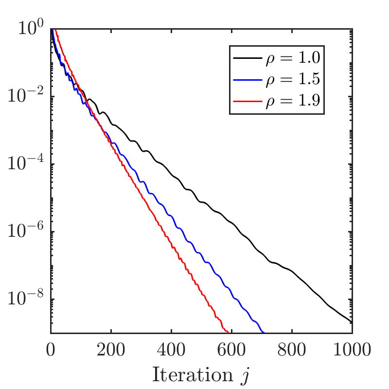
(a) Feasible.

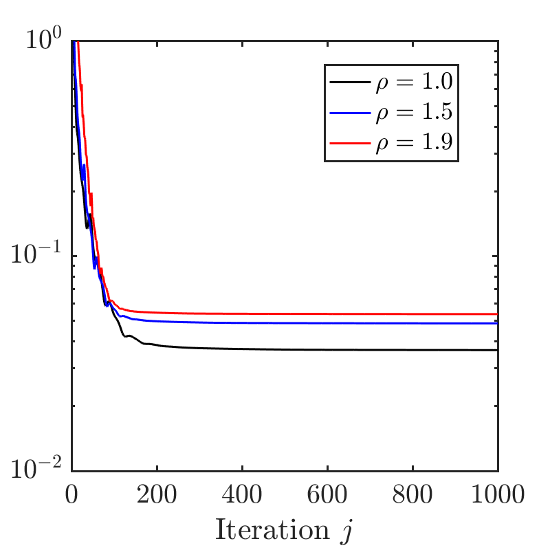
(b) Infeasible.

Figure 3: The asymptotic convergence of $\frac{1}{\beta\rho}\left\lVert w^{j+1}-w^{j}\right\rVert$ in Algorithm 1 when applied to an feasible (left) and infeasible (right) instance of optimization (16).

Table 1: Comparison of the computation time (ms) of different solvers for instances of optimization (16) with randomly sampled values for $\hat{x}_{0}$.

(a) Feasible problems, averaged over 100 random $\hat{x}_{0}$.

$\epsilon_{\text{fea}}$	$l$	OSQP	SCS	ECOS	MOSEK	xPIPG
$10^{-4}$	16	12.9	15.5	63.7	26.8	15.7
	32	60.5	63.5	284.9	96.7	29.5
	64	437.7	449.3	2120.2	175.9	145.9
	128	2788.7	2846.9	20080.3	316.0	401.8
$10^{-8}$	16	22.4	25.1	79.3	33.0	31.8
	32	112.1	102.9	363.3	117.6	61.8
	64	658.8	636.8	2448.6	215.2	269.7
	128	3655.3	3560.2	24860.3	374.6	771.8

(b) Infeasible problems, averaged over 100 random $\hat{x}_{0}$.

$\epsilon_{\text{inf}}$	$l$	OSQP	SCS	ECOS	MOSEK	xPIPG
$10^{-4}$	16	21.9	26.1	47.4	26.2	8.6
	32	97.4	116.9	209.1	103.6	16.1
	64	799.2	845.4	1614.6	185.6	82.1
	128	4545.5	5563.9	13900.3	345.1	233.4
$10^{-8}$	16	33.6	45.7	71.6	51.3	13.6
	32	92.3	118.7	208.3	122.7	16.0
	64	713.7	821.1	1432.0	216.1	56.7
	128	4367.7	5202.7	13611.8	285.9	211.7

5 Conclusions

We introduced a first-order conic optimization method, xPIPG, that automatically detects primal or dual infeasibility in conic optimization. With an efficient C implementation, xPIPG outperforms many state-of-the-art conic optimization solvers especially for large-scale problems.

However, our software implementation and numerical experiments are still limited to a special class of optimal control problems. Our future work direction includes preconditioning and parameter selection in xPIPG for ill-conditioned problems, such as those in the Maros-Meszaros dataset [24, 4].

6 Proof of Lemma 2

Let $\xi_{i}\in\mathbb{R}^{n}$, $\eta_{i}\in\mathbb{R}^{m}$, and

$$z_{i}^{+}= \pi_{\mathbb{D}}[\xi_{i}-\alpha(P\xi_{i}+q+H^{\top}\eta_{i})],$$ (20a)

$$w_{i}^{+}= \pi_{\mathbb{K}^{\circ}}[\eta_{i}+\beta(H(2z_{i}^{+}-\xi_{i})-g)],$$ (20b)

$$\xi_{i}^{+}= (1-\rho)\xi_{i}+\rho z_{i}^{+},\enskip\eta_{i}^{+}=(1-\rho)\eta_{i}+\rho w_{i}^{+},$$ (20c)

for $i=1,2$. By applying [17, Thm. 3.16] to the projections in (20a) and (20b) we can show the following:

$$\textstyle\langle\frac{1}{\alpha}(z_{1}^{+}-\xi_{1})+P\xi_{1}+q+H^{\top}\eta_{1},z_{2}^{+}-z_{1}^{+}\rangle\geq 0,$$ (21a)

$$\textstyle\langle\frac{1}{\alpha}(z_{2}^{+}-\xi_{2})+P\xi_{2}+q+H^{\top}\eta_{2},z_{1}^{+}-z_{2}^{+}\rangle\geq 0,$$ (21b)

$$\textstyle\langle\frac{1}{\beta}(w_{1}^{+}-\eta_{1})-H(2z_{1}^{+}-\xi_{1})+g,w_{2}^{+}-w_{1}^{+}\rangle\geq 0,$$ (21c)

$$\textstyle\langle\frac{1}{\beta}(w_{2}^{+}-\eta_{2})-H(2z_{2}^{+}-\xi_{2})+g,w_{1}^{+}-w_{2}^{+}\rangle\geq 0,$$ (21d)

Summing up (21a) and (21b) gives

$$0\leq\textstyle\frac{1}{\alpha}\langle z_{1}^{+}-z_{2}^{+},\xi_{1}-\xi_{2}-z_{1}^{+}+z_{2}^{+}\rangle$$ (22)

$$-\langle z_{1}^{+}-z_{2}^{+},P(\xi_{1}-\xi_{2})\rangle+\langle z_{1}^{+}-z_{2}^{+},H^{\top}(\eta_{2}-\eta_{1})\rangle.$$

Similarly, summing up (21c) and (21d) gives

$$\textstyle 0\leq\frac{1}{\beta}\langle w_{1}^{+}-w_{2}^{+},\eta_{1}-\eta_{2}-w_{1}^{+}+w_{2}^{+}\rangle$$ (23)

$$-\langle w_{1}^{+}-w_{2}^{+},H(\xi_{1}-\xi_{2}-2z_{1}^{+}+2z_{2}^{+})\rangle.$$

Since matrix $P$ is positive semidefinite, we must have $\langle z_{1}^{+}-z_{2}^{+},P(z_{1}^{+}-z_{2}^{+})\rangle\geq 0$. Using this fact we can show the following

$$-\langle z_{1}^{+}-z_{2}^{+},P(\xi_{1}-\xi_{2})\rangle$$ (24)

$$\leq-\langle z_{1}^{+}-z_{2}^{+},P(\xi_{1}-\xi_{2}-z_{1}^{+}+z_{2}^{+})\rangle.$$

Let

$$\zeta_{1}=\begin{bmatrix}\xi_{1}\\ \eta_{1}\end{bmatrix},\enskip\zeta_{2}=\begin{bmatrix}\xi_{2}\\ \eta_{2}\end{bmatrix},\enskip y_{1}^{+}=\begin{bmatrix}z_{1}^{+}\\ w_{1}^{+}\end{bmatrix},\enskip y_{2}^{+}=\begin{bmatrix}z_{2}^{+}\\ w_{2}^{+}\end{bmatrix}.$$ (25)

Summing up (22), (23), and (24) gives

$$0\leq\langle y_{1}^{+}-y_{2}^{+},\zeta_{1}-\zeta_{2}-y_{1}^{+}+y_{2}^{+}\rangle_{M}.$$ (26)

Next, equation (20c) imply that $\textstyle y_{i}^{+}=\zeta_{i}+\frac{1}{\rho}(\zeta_{i}^{+}-\zeta_{i})$ for $i=1,2$. Substituting this relation into (26) gives

$$\textstyle 0\leq\frac{1}{\rho^{2}}\langle\zeta_{1}^{+}-\zeta_{2}^{+},\zeta_{1}-\zeta_{2}-\zeta_{1}^{+}+\zeta_{2}^{+}\rangle_{M}$$ (27)

$$\textstyle+\frac{1-\rho}{\rho^{2}}\langle\zeta_{1}-\zeta_{2},\zeta_{1}^{+}-\zeta_{2}^{+}-\zeta_{1}+\zeta_{2}\rangle_{M}$$

$$=\textstyle\frac{1}{2\rho^{2}}\left\lVert\zeta_{1}-\zeta_{2}\right\rVert_{M}^{2}-\frac{1}{2\rho^{2}}\left\lVert\zeta_{1}^{+}-\zeta_{2}^{+}\right\rVert_{M}^{2}$$

$$\textstyle-\frac{1}{2\rho^{2}}\left\lVert\zeta_{1}-\zeta_{2}-\zeta_{1}^{+}+\zeta_{2}^{+}\right\rVert_{M}^{2}+\frac{1-\rho}{2\rho^{2}}\left\lVert\zeta_{1}^{+}-\zeta_{2}^{+}\right\rVert_{M}^{2}$$

$$\textstyle-\frac{1-\rho}{2\rho^{2}}\left\lVert\zeta_{1}-\zeta_{2}\right\rVert_{M}^{2}-\frac{1-\rho}{2\rho^{2}}\left\lVert\zeta_{1}-\zeta_{2}-\zeta_{1}^{+}+\zeta_{2}^{+}\right\rVert_{M}^{2}$$

$$=\textstyle\frac{1}{2\rho}\left\lVert\zeta_{1}-\zeta_{2}\right\rVert_{M}^{2}-\frac{1}{2\rho}\left\lVert\zeta_{1}^{+}-\zeta_{2}^{+}\right\rVert_{M}^{2}$$

$$+\textstyle\frac{(\rho-2)}{2\rho^{2}}\left\lVert\zeta_{1}-\zeta_{2}-\zeta_{1}^{+}+\zeta_{2}^{+}\right\rVert_{M}^{2},$$

where the first step is due to completion of squares. Letting $\rho=2\gamma$ for some $\gamma\in(0,1)$ in the inequality above gives (10), which completes the proof.

7 Proof of Theorem 1

We will use the results in [3, Lem. 3.2]. First, by combining Lemma 2 and Lemma 1, we can show that there exists $\overline{z}\in\mathbb{R}^{n}$ and $\overline{w}\in\mathbb{R}^{m}$ such that

$$\textstyle\lim\limits_{j\to\infty}\xi^{j}-\xi^{j-1}=\lim\limits_{j\to\infty}\frac{\xi^{j}}{j}=\overline{z},$$ (28a)

$$\textstyle\lim\limits_{j\to\infty}\eta^{j}-\eta^{j-1}=\lim\limits_{j\to\infty}\frac{\eta^{j}}{j}=\overline{w}.$$ (28b)

Next, line 5 and line 6 in Algorithm 1 implies that $\rho(z^{j}-\xi^{j})=\xi^{j}-\xi^{j-1}$, $z^{j}=\xi^{j-1}+\frac{1}{\rho}(\xi^{j}-\xi^{j-1})$, $\rho(w^{j}-\eta^{j})=\eta^{j}-\eta^{j-1}$, and $w^{j}=\eta^{j-1}+\frac{1}{\rho}(\eta^{j}-\eta^{j-1})$. By combining these equalities with (28), we can show the following:

$$\textstyle\lim\limits_{j\to\infty}z^{j}-z^{j-1}=\lim\limits_{j\to\infty}\rho(z^{j}-\xi^{j-1})=\lim\limits_{j\to\infty}\frac{z^{j}}{j}=\overline{z},$$ (29)

$$\textstyle\lim\limits_{j\to\infty}w^{j}-w^{j-1}=\lim\limits_{j\to\infty}\rho(w^{j}-\eta^{j-1})=\lim\limits_{j\to\infty}\frac{w^{j}}{j}=\overline{w}.$$

The above equation established (12). Our next step is to prove the conditions in (14). By applying [27, Thm. 27.4] to line 3 and line 4 in Algorithm 1, we can show the following:

$$\textstyle\frac{1}{\alpha}(\xi^{j}-z^{j+1})-P\xi^{j}-q-H^{\top}\eta^{j}\in N_{\mathbb{D}}(z^{j+1}),$$ (30a)

$$\textstyle\frac{1}{\beta}(\eta^{j}-w^{j+1})+H(2z^{j+1}-\xi^{j})-g\in N_{\mathbb{K}^{\circ}}(w^{j+1}).$$ (30b)

According to the definition in (4), the distance from point $-Pz^{j+1}-q-Hw^{j+1}$ to the set $N_{\mathbb{D}}(z^{j+1})$ is no larger than the distance from $-Pz^{j+1}-q-Hw^{j+1}$ to $\frac{1}{\alpha}(\xi^{j}-z^{j+1})-P\xi^{j}-q-H^{\top}\eta^{j}$; the reason is because $\frac{1}{\alpha}(\xi^{j}-z^{j+1})-P\xi^{j}-q-H^{\top}\eta^{j}$ is, according to (30a), in set $N_{\mathbb{D}}(z^{j+1})$. In other words, the following inequality holds:

$$d(-Pz^{j+1}-q-Hw^{j+1}|N_{\mathbb{D}}(z^{j+1}))$$ (31)

$$\textstyle\leq\left\lVert(\frac{1}{\alpha}I-P)(z^{j+1}-\xi^{j})-H^{\top}(w^{j+1}-\eta^{j})\right\rVert.$$

Similarly, we can show

$$d(Hz^{j+1}-g|N_{\mathbb{K}^{\circ}}(w^{j+1}))$$ (32)

$$\textstyle\leq\left\lVert\frac{1}{\beta}(w^{j+1}-\eta^{j})-H(z^{j+1}-\xi^{j})\right\rVert.$$

By combining the limits in (29), (31), and (32), we can prove the limits in (14), assuming $\left\lVert\overline{z}\right\rVert=\left\lVert\overline{w}\right\rVert=0$.

We now prove the conditions in (13). To this end, let

$$\hat{z}^{j}=\xi^{j-1}-\alpha(P\xi^{j-1}+q+H^{\top}\eta^{j-1}),$$ (33)

$$\hat{w}^{j}=\eta^{j-1}+\beta(H(2z^{j}-\xi^{j-1})-g).$$

Dividing the above two equalities by $j$ then letting $j\to\infty$ gives the following:

$$\textstyle\lim\limits_{j\to\infty}\frac{\hat{z}^{j}}{j}=\overline{z}-\alpha(P\overline{z}+H^{\top}\overline{w}),\enskip\textstyle\lim\limits_{j\to\infty}\frac{\hat{w}^{j}}{j}=\overline{w}+\beta H\overline{z},$$ (34)

where we again used (29). Since $z^{j}=\pi_{\mathbb{D}}[\hat{z}^{j}]$, $w^{j}=\pi_{\mathbb{K}^{\circ}}[\hat{w}^{j}]$ (due to line 3 and line 4 in Algorithm 1), by using the results in [3, Lem. 3.2] we can show the following:

$$\hat{z}^{j}-z^{j}\in(\mathrm{rec\,}\mathbb{D})^{\circ},\enskip\hat{w}^{j}-w^{j}\in\mathbb{K},$$ (35a)

$$\lim\limits_{j\to\infty}\textstyle\frac{z_{j}}{j}=\overline{z}=\pi_{\mathrm{rec\,}\mathbb{D}}[\overline{z}-\alpha(P\overline{z}+H^{\top}\overline{w})],$$ (35b)

$$\lim\limits_{j\to\infty}\textstyle\frac{w_{j}}{j}=\overline{w}=\pi_{\mathbb{K}^{\circ}}[\overline{w}+\beta H\overline{z}],$$ (35c)

$$\begin{aligned} \lim\limits_{j\to\infty}\textstyle\frac{\hat{z}^{j}-z^{j}}{j}&=\pi_{(\mathrm{rec\,}\mathbb{D})^{\circ}}[\overline{z}-\alpha(P\overline{z}+H^{\top}\overline{w})]\\ &=-\alpha(P\overline{z}+H^{\top}\overline{w}),\end{aligned}$$ (35d)

$$\lim\limits_{j\to\infty}\textstyle\frac{\hat{w}^{j}-w^{j}}{j}=\pi_{\mathbb{K}}[\overline{w}+\beta H\overline{z}]=\beta H\overline{z},$$ (35e)

$$\lim\limits_{j\to\infty}\textstyle\frac{\langle z^{j},\hat{z}^{j}-z^{j}\rangle}{j}=\sigma_{\mathbb{D}}[-\alpha(P\overline{z}+H^{\top}\overline{w})],$$ (35f)

$$\lim\limits_{j\to\infty}\textstyle\frac{\langle w^{j},\hat{w}^{j}-w^{j}\rangle}{j}=\sigma_{\mathbb{K}^{\circ}}[\beta H\overline{z}]=0,$$ (35g)

where we used the fact that $\mathrm{rec\,}\mathbb{K}^{\circ}=\mathbb{K}^{\circ}$ and $(\mathbb{K}^{\circ})^{\circ}=\mathbb{K}$; we also used (29) and (34) in (35d) and (35e). Notice that (35b), (35c), and (35e) directly implies the following

$$\overline{z}\in\mathrm{rec\,}\mathbb{D},\enskip\overline{w}\in\mathbb{K}^{\circ},\enskip H\overline{z}\in\mathbb{K}.$$ (36)

By applying [17, Thm. 6.30] to the projections in (35b), (35d), (35c), and (35e) we can show the following

$$\langle\overline{z},P\overline{z}+H^{\top}\overline{w}\rangle=0,$$ (37a)

$$\langle\overline{w},H\overline{z}\rangle=0.$$ (37b)

Combining the above two equalities with the assumption that $P$ is positive semidefinite, we can conclude that

$$P\overline{z}=0.$$ (38)

Next, we proceed to prove the conditions in (13) (other than those in (36) and (38)) using two argument. In the first argument, we start with the following:

$$\langle w^{j},H\overline{z}\rangle\leq\langle-P\xi^{j-1},\overline{z}\rangle,$$ (39a)

$$\langle-Hz^{j},\overline{w}\rangle\leq\sigma_{\mathbb{D}}(-H^{\top}\overline{w}),$$ (39b)

where (39a) is due to (36), (38), and the definition of polar cone in (9); (39b) is due to (8).

Furthermore, by using (33), (35a), (35b), (35c), and the definition in (9) we can show the following

$$\textstyle\langle\frac{1}{\alpha}(\xi^{j-1}-z^{j})-P\xi^{j-1}-q-H^{\top}\eta^{j-1},\overline{z}\rangle\leq 0,$$ (40a)

$$\textstyle\langle\frac{1}{\beta}(\eta^{j-1}-w^{j})+H(2z^{j}-\xi^{j-1})-g,\overline{w}\rangle\leq 0.$$ (40b)

By first summing up both sides of (39a) and (40a), then letting $j\to\infty$, we can show the following

$$\textstyle\frac{1}{\rho\alpha}\left\lVert\overline{z}\right\rVert^{2}+\langle q,\overline{z}\rangle\geq\textstyle\frac{1}{\rho}\langle H\overline{z},\overline{w}\rangle=0,$$ (41)

where we also used (29) and(37b). Similarly, by first summing both sides of (39b) and (40b), then letting $j\to\infty$, we can show the following

$$\textstyle\frac{1}{\rho\beta}\left\lVert\overline{w}\right\rVert^{2}+\langle g,\overline{w}\rangle+\sigma_{\mathbb{D}}(-H^{\top}\overline{w})\geq\textstyle\frac{1}{\rho}\langle H\overline{z},\overline{w}\rangle=0,$$ (42)

where the last step is due to (37b).

Finally, by summing up both sides of (41) and (42), we obtain the following intermediate step:

$$\textstyle\sigma_{\mathbb{D}}(-H^{\top}\overline{w})+\langle q,\overline{z}\rangle+\langle g,\overline{w}\rangle+\frac{1}{\rho\alpha}\left\lVert\overline{z}\right\rVert^{2}+\frac{1}{\rho\beta}\left\lVert\overline{w}\right\rVert^{2}\geq 0.$$ (43)

Inequality (43) completes our first argument. In the second argument, we will show that the inequality in (43) actually holds as an equality, using the following three steps. First, combining (29) and (34) gives the following

$$\lim\limits_{j\to\infty}\textstyle\frac{1}{\alpha j}\langle z^{j}-\hat{z}^{j},z^{j}-\xi^{j-1}\rangle=\frac{1}{\rho}\langle P\overline{z}+H^{\top}\overline{w},\overline{z}\rangle=0,$$ (44)

$$\lim\limits_{j\to\infty}\textstyle\frac{1}{\beta j}\langle w^{j}-\hat{w}^{j},w^{j}-\eta^{j-1}\rangle=\frac{1}{\rho}\langle H\overline{z},\overline{w}\rangle=0.$$

where the last step in the above two inequalities are due to (37b) and (38). Second, by using (33) we can show the following

$$\textstyle\frac{1}{\alpha j}\langle z^{j}-\hat{z}^{j},\xi^{j-1}\rangle$$ (45)

$$\geq\textstyle\frac{1}{j}\langle\frac{1}{\alpha}(z^{j}-\xi^{j-1})+q+H^{\top}\eta^{j-1},\xi^{j-1}\rangle,$$

where we used the assumption that $P$ is positive semidefinite. Similarly, by using (33) we can show the following

$$\textstyle\frac{1}{\beta j}\langle w^{j}-\hat{w}^{j},\eta^{j-1}\rangle$$ (46)

$$=\textstyle\frac{1}{j}\langle\frac{1}{\beta}(w^{j}-\eta^{j-1})-H(2z^{j}-\xi^{j-1})+g,\eta^{j-1}\rangle.$$

Third, by first summing up the both sides of (45), and (46), then letting $j\to\infty$, we obtain the following

$$\textstyle\frac{1}{\alpha\rho}\left\lVert\overline{z}\right\rVert^{2}+\frac{1}{\beta\rho}\left\lVert\overline{w}\right\rVert^{2}+\langle q,\overline{z}\rangle+\langle g,\overline{w}\rangle-\frac{2}{\rho}\langle H\overline{z},\overline{w}\rangle$$ (47)

$$\leq\lim\limits_{j\to\infty}\textstyle\frac{1}{\alpha j}\langle z^{j}-\hat{z}^{j},\xi^{j-1}\rangle+\lim\limits_{j\to\infty}\textstyle\frac{1}{\beta j}\langle w^{j}-\hat{w}^{j},\eta^{j-1}\rangle,$$

Notice the two limits in (47) always exist, due to (35f), (35g), and (44). By combining (47) together with (44), (35f), (35g), and (37b) we obtain can the following

$$\textstyle\sigma_{\mathbb{D}}(-H^{\top}\overline{w})+\langle q,\overline{z}\rangle+\langle g,\overline{w}\rangle+\frac{1}{\rho\alpha}\left\lVert\overline{z}\right\rVert^{2}+\frac{1}{\rho\beta}\left\lVert\overline{w}\right\rVert^{2}\leq 0,$$ (48)

where we also used (38) and the fact that $\sigma_{\mathbb{D}}(-\alpha H^{\top}\overline{w})=\alpha\sigma_{\mathbb{D}}(-H^{\top}\overline{w})$ for any $\alpha\geq 0$. By combining (43) and (48) we conclude that inequality (43) holds as an equality. Consequently, the inequalities in (41) and (42) must also hold as equalities, i.e.,

$$\textstyle\langle q,\overline{z}\rangle=-\frac{1}{\rho\alpha}\left\lVert\overline{z}\right\rVert^{2},\enskip\textstyle\sigma_{\mathbb{D}}(-H^{\top}\overline{w})+\langle g,\overline{w}\rangle=-\frac{1}{\rho\beta}\left\lVert\overline{w}\right\rVert^{2}.$$ (49)

We now finished our second argument. Finally, by combining (36), the second equality in (49), and the fact that $\langle\overline{w},y\rangle\leq 0$ for all $y\in\mathbb{K}$–which is due to $\overline{w}\in\mathbb{K}^{\circ}$ in (36)–we can obtain (13a). By combining (36), (38), and the first equality in (49), we can obtain (13b).

References

[1]
B. O’Donoghue, E. Chu, N. Parikh, and S. Boyd, “Conic optimization via
operator splitting and homogeneous self-dual embedding,” J. Optim.
Theory Appl., vol. 169, no. 3, pp. 1042–1068, 2016.
[2]
G. Banjac, P. Goulart, B. Stellato, and S. Boyd, “Infeasibility detection in
the alternating direction method of multipliers for convex optimization,”
J. Optim. Theory Appl., vol. 183, no. 2, pp. 490–519, 2019.
[3]
G. Banjac and J. Lygeros, “On the asymptotic behavior of the
Douglas–Rachford and proximal-point algorithms for convex
optimization,” Optim. Lett., pp. 1–14, 2021.
[4]
B. O’Donoghue, “Operator splitting for a homogeneous embedding of the linear
complementarity problem,” SIAM J. Optim., vol. 31, no. 3, pp.
1999–2023, 2021.
[5]
Y. Yu and U. Topcu, “Proportional-integral projected gradient method for
infeasibility detection in conic optimization,” arXiv preprint
arXiv:2109.02756[math.OC], 2021.
[6]
D. Applegate, M. Díaz, H. Lu, and M. Lubin, “Infeasibility detection with
primal-dual hybrid gradient for large-scale linear programming,” arXiv
preprint arXiv:2102.04592[math.OC], 2021.
[7]
G. Banjac, “On the minimal displacement vector of the Douglas–Rachford
operator,” Oper. Res. Lett., vol. 49, no. 2, pp. 197–200, 2021.
[8]
Y. Nesterov, M. J. Todd, and Y. Ye, “Infeasible-start primal-dual methods and
infeasibility detectors for nonlinear programming problems,” Math.
Program., vol. 84, no. 2, pp. 227–268, 1999.
[9]
A. U. Raghunathan and S. Di Cairano, “Infeasibility detection in alternating
direction method of multipliers for convex quadratic programs,” in
Proc. IEEE Conf. Decision Control. IEEE, 2014, pp. 5819–5824.
[10]
Y. Liu, E. K. Ryu, and W. Yin, “A new use of Douglas–Rachford splitting
for identifying infeasible, unbounded, and pathological conic programs,”
Math. Program., vol. 177, no. 1, pp. 225–253, 2019.
[11]
E. K. Ryu, Y. Liu, and W. Yin, “Douglas–Rachford splitting and ADMM for
pathological convex optimization,” Comput. Optim. Appl., vol. 74,
no. 3, pp. 747–778, 2019.
[12]
A. Chambolle and T. Pock, “On the ergodic convergence rates of a first-order
primal–dual algorithm,” Math. Program., vol. 159, no. 1-2, pp.
253–287, 2016.
[13]
Y. Yu, P. Elango, and B. Açıkmeşe, “Proportional-integral
projected gradient method for model predictive control,” IEEE Control
Syst. Lett., vol. 5, no. 6, pp. 2174–2179, 2020.
[14]
Y. Yu, P. Elango, U. Topcu, and B. Açıkmeşe,