Bispectrum-window convolution via Hankel transform

Abstract

We present a method to perform the exact convolution of the model prediction for bispectrum multipoles in redshift space with the survey window function. We extend a widely applied method for the power spectrum convolution to the bispectrum, taking advantage of a 2D-FFTlog algorithm. As a preliminary test of its accuracy, we consider the toy model of a spherical window function in real space. This setup provides an analytical evaluation of the 3-point function of the window, and therefore it allows to isolate and quantify possible systematic errors of the method. We find that our implementation of the convolution in terms of a mixing matrix shows differences at the percent level in comparison to the measurements from a very large set of mock halo catalogs. It is also able to recover unbiased constraints on halo bias parameters in a likelihood analysis of a set of numerical simulations with a total volume of $100\,h^{-3}\,{\rm Gpc}^{3}$. For the level of accuracy required by these tests, the multiplication with the mixing matrix is performed in the time of one second or less.

1 Introduction

One particular class of observables to study galaxy clustering are three-dimensional, Fourier-space summary statistics of the galaxy distribution [1]. For a Gaussian distribution, all statistical properties are encoded in its power spectrum. However, non-Gaussianity, quantified in non-vanishing, higher-order correlation functions, is induced by gravitational instability, nonlinear bias and redshift-space distortions. The measurement of the galaxy bispectrum, i.e. the three-point function of the galaxy distribution in Fourier space, is therefore expected to complement a power spectrum-only analysis. Such a combined analysis offers specific information on the parameters controlling nonlinear corrections to the power spectrum itself [2, 3, 4, 5, 6, 7, 8, 9, 10, 11, 12, 13, 14, 15]. In addition, the galaxy bispectrum can directly probe a primordial non-Gaussian component, possibly shedding light on the interactions taking place during inflation [16, 17, 18, 19, 20, 21, 22, 23, 24, 25, 26] . Recent efforts using measurements of the galaxy bispectrum in BOSS are the first steps toward this direction [27, 28].

The analysis of higher-order statistics comes at the price of greater complexity in their measurement, modelling and estimation of their covariance properties. A specific challenge comes from the fact that the conventional FKP-like estimator [29, 30, 31] (extending the Feldman-Kaiser-Peacock power spectrum estimator of [32]) used in spectroscopic surveys provides as output a non trivial convolution of the underlying galaxy bispectrum with the survey footprint and redshift selection function. The estimator actually computes the three-point function of the Fourier Transform of the product between the galaxy overdensity $\delta(\mathbf{x})$ and the window function $W(\mathbf{x})$, vanishing outside the observed volume. Consequently, the theoretical model for the bispectrum $B(\mathbf{k}_{1},\mathbf{k}_{2})$ has be to convolved with the bispectrum of the window $B_{W}(\mathbf{k}_{1},\mathbf{k}_{2})\equiv W(\mathbf{k}_{1})W(\mathbf{k}_{2})W^{*}(\mathbf{k}_{1}+\mathbf{k}_{2})$ to obtain

$$\tilde{B}(\mathbf{k}_{1},\mathbf{k}_{2})=\int\frac{d^{3}p_{1}}{(2\pi)^{3}}\int\frac{d^{3}p_{2}}{(2\pi)^{3}}B_{W}(\mathbf{k}_{1}-\mathbf{p}_{1},\mathbf{k}_{2}-\mathbf{p}_{2})B(\mathbf{p}_{1},\mathbf{p}_{2})\,,$$ (1.1)

that is the quantity to be compared with the measurement. A fast evaluation of this type of integral, for example in terms of mixing matrix relating $B$ to $\tilde{B}$, is required for a likelihood analyses, where the matrix multiplication has to be done for each point sampled in the parameter space.

In the case of the power spectrum, a formulation that turns the convolution integral into a series of one-dimensional Hankel transforms has been proposed by [33]. This was later expanded by [34] to the case of the local plane-parallel estimator of [35, 36, 31] and to include wide-angle and general-relativistic effects [37, 38, 39]. The core technique of this method relies on the FFTLog algorithm [40], an implementation of the Fast-Fourier Tranform algorithm on logarithmically-spaced points. The Hankel-transform formulation speeds-up the process considerably, as it amounts to evaluating a one-dimensional FFT, scaling as $N\log N$ for $N$ sample points, instead of the full three-dimensional FFT. However, the FFTLog algorithm suffers from the typical FFT problems such as aliasing and ringing, which might give spurious effects if not treated carefully. The formulation in terms of a matrix multiplication, schematically written as $\tilde{P}_{\ell}(\mathbf{k})=\mathcal{W}_{\ell\ell^{\prime}}(\mathbf{k},\mathbf{p})P_{\ell^{\prime}}(\mathbf{p})$ [10, 41, 42] transfers the FFTLog calculation in the matrix $\mathcal{W}_{\ell\ell^{\prime}}(\mathbf{k},\mathbf{p})$ that can be pre-computed and tested carefully.

The bispectrum convolution received so far, understandably, less attention. References [43, 44, 45] considered, for a galaxy bispectrum monopole measured according to [31], an approximation that ignores the effect of the convolution of the nonlinear kernel characterizing the tree-level prediction for the bispectrum. This approach works quite well on most triangle shapes, except for squeezed configurations where one side is comparable to the inverse of the characteristic size of the window, $1/R$. This could lead to discarding potentially valuable information on large scales, as we can expect, for instance, in models with local primordial non-Gaussianity [46].

An alternative is to consider an entirely different estimator. An example is the tri-polar spherical harmonics (TripoSH) estimator proposed by [47], that uses the tensor product of three spherical harmonics as a basis for a bispectrum decomposition. This estimator is the natural extension of the real-space bispectrum estimator for the quantity $B_{\ell}(k_{1},k_{2})$, function of the two wavevectors $(k_{1},k_{2})$ and the multipole index $\ell$ characterizing the angle between $\mathbf{k}_{1}$ and $\mathbf{k}_{2}$. This decomposition has been shown to be computable via two-dimensional Hankel transforms of its three point function multipoles [48]. However, this estimator requires special care with the truncation for the multipoles expansion of bispectrum, since in general this decomposition requires an infinite number of multipoles [49].

Another type of estimator recently proposed is the cubic estimator of [50], which bypasses the need of the window convolution of the theoretical modelling altogether. This estimator falls under the class of maximum-likelihood estimators [51, 52, 53, 54] which, by construction, approach the Cramér-Rao bound on the information content of a given bandpower. This is certainly a very promising way to measure the bispectrum, but it still lacks an analytical understanding of why such estimators, even for the power spectrum, are unbiased in wide field galaxy surveys.

Our approach in this work is to provide a theoretical prediction for the redshift-space bispectrum multipoles estimator of [31], which is a natural extension of the FFT-based, variable line-of-sight estimator of the power spectrum estimator [32, 5, 36, 31]. Our goal is to write such a convolution as a matrix multiplication, with the mixing matrix computable via a multidimensional Hankel transform.

This work is organized as follows. A description of the bispectrum estimator that we adopt is presented in section 2. The bispectrum-window convolution formulation in terms of Hankel transform is laid out in section 3. We present the setup of an ideal test in terms of a spherical window in real space in section 4 while we show the results of the test in section 5. Finally, we present our conclusions in section 6.

2 Bispectrum multipoles estimator

We consider the definition of the redshift-space bispectrum multipoles introduced by [29] where the orientation of the triangle formed by the wavenumbers $\mathbf{k}_{1}$, $\mathbf{k}_{2}$, $\mathbf{k}_{3}$, is parameterized in terms of the angle $\theta$ between $\mathbf{k}_{1}$ and the line-of-sight and of the angle $\phi$ describing the rotation of $\mathbf{k}_{2}$ around $\mathbf{k}_{1}$ (see [55] for an alternative choice). Expanding this angle-dependence in spherical harmonics $Y_{LM}(\theta,\phi)$, the corresponding multipoles are given by

$$B_{LM}(k_{1},k_{2},k_{3})=\int\!\!d\!\cos{\theta}\int\!\!d\phi B(k_{1},k_{2},k_{3},\theta,\phi)\,Y_{LM}(\theta,\phi)\,.$$ (2.1)

In practice, we restrict our attention to an expansion in Legendre polynomials ${\mathcal{L}}_{L}(\cos\theta)$ of the bispectrum averaged over the angle $\phi$, as it is often the case (see [8] for motivation). These are defined as

$$B_{L}(k_{1},k_{2},k_{3}) =\sqrt{\frac{2L+1}{4\pi}}\,B_{L0}(k_{1},k_{2},k_{3})$$

$$=\frac{2L+1}{4\pi}\int\!\!d\!\cos{\theta}\int d\phi B(k_{1},k_{2},k_{3},\theta,\phi)\,\mathcal{L}_{L}(\cos\theta)\,.$$ (2.2)

The estimator proposed by [31] can be written as

$$\hat{B}_{L}(k_{1},k_{2},k_{3})=\frac{2L+1}{V_{B}}\int_{k_{1}}\!\!d^{3}q_{1}\!\!\int_{k_{2}}\!\!d^{3}q_{2}\!\!\int_{k_{3}}\!\!d^{3}q_{3}~{}\delta_{D}(\mathbf{q}_{123})\int d^{3}x\,\hat{B}^{\rm local}(\mathbf{q}_{1},\mathbf{q}_{2};\mathbf{x})\,{\mathcal{L}}_{L}(\hat{q}_{1}\cdot\hat{x})\,,$$ (2.3)

where the integration $\int_{k}d^{3}q$ is taken over the spherical shell of radius in the range $k-\Delta k/2\leq q\leq k+\Delta k/2$ for the bin width $\Delta k$ and where

$$V_{B}(k_{1},k_{2},k_{3})\equiv\int_{k_{1}}\!\!d^{3}q_{1}\!\!\int_{k_{2}}\!\!d^{3}q_{2}\!\!\int_{k_{3}}\!\!d^{3}q_{3}~{}\delta_{D}(\mathbf{q}_{123})\,,$$ (2.4)

adopting the notation for wavevector sums $\mathbf{q}_{ij}\equiv\mathbf{q}_{i}+\mathbf{q}_{j}$. The local bispectrum estimator

$$\hat{B}^{\rm local}(\mathbf{q}_{1},\mathbf{q}_{2};\mathbf{x})=\int d^{3}x_{13}\int d^{3}x_{23}~{}e^{-i\mathbf{q}_{1}\cdot\mathbf{x}_{13}}e^{-i\mathbf{q}_{2}\cdot\mathbf{x}_{23}}\delta(\mathbf{x}_{1})\delta(\mathbf{x}_{2})\delta(\mathbf{x}_{3})$$ (2.5)

with $\mathbf{x}_{ij}=\mathbf{x}_{i}-\mathbf{x}_{j}$, corresponds to the Fourier Transform of the product $\delta(\mathbf{x}_{1})\delta(\mathbf{x}_{2})\delta(\mathbf{x}_{3})$ where the mean point $\mathbf{x}=(\mathbf{x}_{1}+\mathbf{x}_{2}+\mathbf{x}_{3})/3$ provides the direction of the line-of-sight $\hat{n}$, so that $\cos\theta\equiv\hat{q}_{1}\cdot\hat{x}$ .

By replacing $\mathbf{x}\rightarrow\mathbf{x}_{3}$, the integrand in eq. (2.3) becomes separable, thus enabling an efficient computation via linear combination of Fast Fourier Transforms. The differences induced in the measurements (and hence in the predictions) between these two definitions of the line-of-sight, the so-called wide angle effects, are usually negligible in the modelling of the power multipoles spectrum in a typical galaxy survey. We will assume the same is true for the bispectrum, although we acknowledge that a quantitative study of wide angle effects in the bispectrum is missing.

3 Window convolution via Hankel Transform

In a cosmological analysis we need to compare the measurements of the estimator in eq. (2.3) to the corresponding theoretical prediction, that is the ensemble average $\tilde{B}_{L}\equiv\langle\hat{B}_{L}\rangle$. Replacing $\delta(\mathbf{x})\rightarrow\delta(\mathbf{x})\,W(\mathbf{x})$, with $W(\mathbf{x})$ representing here the window as a purely geometrical step function taking values 0 or 1, we obtain

$$\tilde{B}_{L}(k_{1},k_{2},k_{3}) =\frac{2L+1}{V_{B}}\int_{k_{1}}\!\!d^{3}q_{1}\!\!\int_{k_{2}}\!\!d^{3}q_{2}\!\!\int_{k_{3}}\!\!d^{3}q_{3}\,\delta_{D}(\mathbf{q}_{123})$$

$$\times\int\!\!d^{3}x_{3}\!\int\!\!d^{3}x_{13}\!\int\!\!d^{3}x_{23}\,e^{-i\mathbf{q}_{1}\cdot\mathbf{x}_{13}}e^{-i\mathbf{q}_{2}\cdot\mathbf{x}_{23}}\zeta(\mathbf{x}_{13},\mathbf{x}_{23},\hat{x}_{3})$$

$$\times W(\mathbf{x}_{1})\,W(\mathbf{x}_{2})\,W(\mathbf{x}_{3})\,\mathcal{L}_{L}(\hat{q}_{1}\cdot\hat{x}_{3})\,,$$ (3.1)

where $\zeta(\mathbf{x}_{13},\mathbf{x}_{23},\hat{x}_{3})$ is the galaxy three-point correlation function (3PCF), and its orientation is defined w.r.t. the line-of-sight direction $\hat{x}_{3}$.

By repeated use of the Rayleigh expansion of a plane wave eq. (D.2), the addition of spherical harmonics eq. (D.3), and the orthogonality of Legendre polynomials eq. (D.4), we can perform the angular integration of the wavevector modes to get

$$\tilde{B}_{L}(k_{1},k_{2},k_{3}) =\frac{8(4\pi)^{2}}{V_{B}}\int_{k_{1}}dq_{1}q_{1}^{2}\int_{k_{2}}dq_{2}q_{2}^{2}\int_{k_{3}}dq_{3}q_{3}^{2}\int d^{3}x\int d^{3}x_{3}\int d^{3}x_{13}\int d^{3}x_{23}$$

$$\times\sum_{\begin{subarray}{c}\ell,\ell_{1},\ell_{2}\\ m,m_{1},M\end{subarray}}i^{\ell-\ell_{1}}(2\ell_{2}+1)j_{0}(q_{3}x)j_{\ell}(q_{1}x)j_{\ell_{2}}(q_{2}x)j_{\ell_{1}}(q_{1}x_{13})j_{\ell_{2}}(q_{2}x_{23})$$

$$\times\mathcal{G}_{L\ell_{1}\ell}^{Mm_{1}m}Y_{\ell_{1}m_{1}}^{*}(\hat{x}_{13})Y_{\ell m}^{*}(\hat{x})Y_{LM}^{*}(\hat{x}_{3})\mathcal{L}_{\ell_{2}}(\hat{x}\cdot\hat{x}_{23})$$

$$\times\zeta(\mathbf{x}_{13},\mathbf{x}_{23},\hat{x}_{3})~{}W(\mathbf{x}_{1})W(\mathbf{x}_{2})W(\mathbf{x}_{3})\,,$$ (3.2)

where we have also used the integration of the product of three spherical harmonics eq. (D.8) resulting in a Gaunt coefficient, eq. (D.10). Performing the angular integration of the dummy variable $\hat{x}$ using the addition and orthogonality of spherical harmonics, eq.s (D.3) and (D.6), we arrive at

$$\tilde{B}_{L}(k_{1},k_{2},k_{3}) =\frac{8(4\pi)^{2}i^{L}}{V_{B}}\int_{k_{1}}dq_{1}q_{1}^{2}\int_{k_{2}}dq_{2}q_{2}^{2}\int_{k_{3}}dq_{3}q_{3}^{2}\int d^{3}x_{3}\int d^{3}x_{13}\int d^{3}x_{23}$$

$$\times\sum_{\begin{subarray}{c}\ell_{1},\ell_{2}\\ M,m_{1},m_{2}\end{subarray}}i^{\ell_{2}-\ell_{1}}I_{\ell_{2}\ell_{2}0}(q_{1},q_{2},q_{3})j_{\ell_{1}}(q_{1}x_{13})j_{\ell_{2}}(q_{2}x_{23})$$

$$\times\mathcal{G}^{Mm_{1}m_{2}}_{L\ell_{1}\ell_{2}}Y_{LM}^{*}(\hat{x}_{3})Y_{\ell_{1}m_{1}}^{*}(\hat{x}_{13})Y_{\ell_{2}m_{2}}^{*}(\hat{x}_{23})~{}\zeta(\mathbf{x}_{13},\mathbf{x}_{23},\hat{x}_{3})~{}W_{1}W_{2}W_{3}\,,$$ (3.3)

where we introduce the integral

$$I_{\ell_{1}\ell_{2}\ell_{3}}(q_{1},q_{2},q_{3})\equiv 4\pi\int dxx^{2}j_{\ell_{1}}(q_{1}x)j_{\ell_{2}}(q_{2}x)j_{\ell_{3}}(q_{3}x).$$ (3.4)

The formulation that we seek is a window convolution expressed in terms of a matrix multiplication of the unconvolved bispectrum with a mixing matrix computable via Hankel transforms. Therefore, we need to transform back, and write the 3PCF in terms of the unconvolved, redshift-space bispectrum $B(\mathbf{p}_{1},\mathbf{p}_{2},\hat{x})$. In turn, the latter can be expanded in spherical harmonics as

$$B(\mathbf{p}_{1},\mathbf{p}_{2},\hat{x}_{3})=\sum_{L^{\prime}M^{\prime}}\bar{B}_{L^{\prime}M^{\prime}}(p_{1},p_{2},p_{3})Y_{L^{\prime}M^{\prime}}(\hat{p}_{1}\cdot\hat{x}_{3},\varphi)\,,$$ (3.5)

where now we consider the azimuthal angle $\varphi$ describing the rotation of $\hat{x}_{3}$ around $\hat{p}_{1}$. It can be easily shown that the coefficients $\bar{B}_{LM}$ of this expansion are related to those defined in eq. (2.1) via $\bar{B}_{LM}=(-1)^{M}B_{L,-M}$ so that

$$B(\mathbf{p}_{1},\mathbf{p}_{2},\hat{x}_{3})=\sum_{L^{\prime}M^{\prime}}B_{L^{\prime},-M^{\prime}}(p_{1},p_{2},p_{3})(-1)^{M^{\prime}}Y_{L^{\prime}M^{\prime}}(\hat{p}_{1}\cdot\hat{x}_{3},\varphi)\,.$$ (3.6)

We can therefore write

$$\zeta(\mathbf{x}_{13},\mathbf{x}_{23},\hat{x}_{3})= \int\!\frac{d^{3}p_{1}}{(2\pi)^{3}}\int\!\frac{d^{3}p_{2}}{(2\pi)^{3}}\int\!\frac{d^{3}p_{3}}{(2\pi)^{3}}e^{i\mathbf{p}_{1}\cdot\mathbf{x}_{13}}e^{i\mathbf{p}_{2}\cdot\mathbf{x}_{23}}B(p_{1},p_{2},p_{3},\hat{x}_{3})(2\pi)^{3}\delta_{D}(\mathbf{p}_{123})$$

$$= \int\!\frac{d^{3}p_{1}}{(2\pi)^{3}}\int\!\frac{d^{3}p_{2}}{(2\pi)^{3}}\int\!\frac{dp_{3}}{2\pi^{2}}p_{3}^{2}~{}e^{i\mathbf{p}_{1}\cdot\mathbf{x}_{13}}e^{i\mathbf{p}_{2}\cdot\mathbf{x}_{23}}B(p_{1},p_{2},p_{3},\hat{x}_{3})$$

$$\times\sum_{\ell}4\pi(-1)^{\ell}(2\ell+1)\int dx~{}x^{2}j_{\ell}(p_{1}x)j_{\ell}(p_{2}x)j_{0}(p_{3}x)\mathcal{L}_{\ell}(\hat{p}_{1}\cdot\hat{p}_{2})$$

$$= \int\!\frac{dp_{1}}{2\pi^{2}}p_{1}^{2}\int\!\frac{dp_{2}}{2\pi^{2}}p_{2}^{2}\int\!\frac{dp_{3}}{2\pi^{2}}p_{3}^{2}\sum_{L^{\prime}M^{\prime}}B_{L^{\prime},-M^{\prime}}(p_{1},p_{2},p_{3})(-1)^{M^{\prime}}$$

$$\times\sum_{\ell}I_{\ell\ell 0}(p_{1},p_{2},p_{3})\sum_{mm^{\prime}\ell^{\prime}}4\pi i^{\ell^{\prime}-\ell}~{}\mathcal{G}_{L^{\prime}\ell\ell^{\prime}}^{M^{\prime}mm^{\prime}}$$

$$\times j_{\ell^{\prime}}(p_{1}x_{13})j_{\ell}(p_{2}x_{23})Y^{*}_{\ell^{\prime}m^{\prime}}(\hat{x}_{13})Y^{*}_{\ell m}(\hat{x}_{23})\,,$$ (3.7)

where we have used the contraction of spherical harmonics eq. (D.12) and the integration of spherical harmonics along solid angle eq. (D.7) to simplify the integral. Plugging back eq. (3) into eq. (3) gives us our final expression for window convolution of the bispectrum as a matrix multiplication

$$\tilde{B}_{L}(k_{1},k_{2},k_{3})= \int\frac{dp_{1}}{2\pi^{2}}p_{1}^{2}\int\frac{dp_{2}}{2\pi^{2}}p_{2}^{2}\int\frac{dp_{3}}{2\pi^{2}}p_{3}^{2}~{}\sum_{L^{\prime}M^{\prime}}B_{L^{\prime}M^{\prime}}(p_{1},p_{2},p_{3})$$

$$\times\sum_{\ell}I_{\ell\ell 0}(p_{1},p_{2},p_{3})\mathcal{Q}_{L^{\prime}M^{\prime}\ell}^{L}(k_{1},k_{2},k_{3};p_{1},p_{2})\,,$$ (3.8)

where the matrix elements are intended to be the triplets $\{p_{1},p_{2},p_{3}\}$. The mixing matrix is given in terms of a product where the first factor is the $I_{\ell\ell 0}(p_{1},p_{2},p_{3})$ function of eq. (3.4) that enforces the triangle condition on $\{p_{1},p_{2},p_{3}\}$ [56]. This can be written as

$$I_{\ell\ell 0}(x,y,z)=(-1)^{\ell}\frac{\pi^{2}}{xyz}\theta(|\hat{x}\cdot\hat{y}|)\mathcal{L}_{\ell}\Big{(}\frac{z^{2}-x^{2}-y^{2}}{2xy}\Big{)}\,,$$ (3.9)

where $\theta(\Delta)$ is the (modified) Heaviside step function that takes value of 1 for $\Delta<1$, 1/2 for $\Delta=1$ while vanishing everywhere else. The window function contribution is accounted for by the second factor, defined as follows

$$\mathcal{Q}^{L}_{L^{\prime}M^{\prime}\ell}(k_{1},k_{2},k_{3};p_{1},p_{2})\equiv \sum_{\ell_{1},\ell_{2},\ell^{\prime}}\frac{128\pi^{2}}{V_{B}}\int_{k_{1}}dq_{1}q_{1}^{2}\int_{k_{2}}dq_{2}q_{2}^{2}\int_{k_{3}}dq_{3}q_{3}^{2}~{}I_{\ell_{2}\ell_{2}0}(q_{1},q_{2},q_{3})$$

$$\times\mathcal{W}^{L}_{L^{\prime}M^{\prime}\ell\ell^{\prime}\ell_{1}\ell_{2}}(q_{1},q_{2};p_{1},p_{2})\,,$$ (3.10)

where we introduce the function

$$\mathcal{W}^{L}_{L^{\prime}M^{\prime}\ell\ell^{\prime}\ell_{1}\ell_{2}}(q_{1},q_{2};p_{1},p_{2})\equiv \,(4\pi)^{2}\int\!dx_{13}\,x_{13}^{2}\int\!dx_{23}\,x_{23}^{2}\,j_{\ell^{\prime}}(p_{1}x_{13})\,j_{\ell}(p_{2}x_{23})$$

$$\times\Big{[}j_{\ell_{1}}(q_{1}x_{13})\,j_{\ell_{2}}(q_{2}x_{23})\,Q^{L}_{L^{\prime}M^{\prime}\ell\ell^{\prime}\ell_{1}\ell_{2}}(x_{13},x_{23})\Big{]}\,,$$ (3.11)

that can be evaluated as a two-dimensional Hankel Transform of the product of two spherical Bessel functions with the 3PCF multipoles of the window function defined as follows

$$Q^{L}_{L^{\prime}M^{\prime}\ell\ell^{\prime}\ell_{1}\ell_{2}}(x_{13},x_{23})\equiv (-1)^{M^{\prime}}\sum_{\tilde{\ell}_{1},\tilde{\ell}_{2}}\sum_{\begin{subarray}{c}M,m_{1},m_{2}\\ m,m^{\prime},\tilde{m}_{1},\tilde{m}_{2}\end{subarray}}4\pi i^{\ell^{\prime}-\ell+\ell_{2}-\ell_{1}}\,\mathcal{G}_{L\ell_{1}\ell_{2}}^{Mm_{1}m_{2}}\,\mathcal{G}_{L^{\prime}\ell\ell^{\prime}}^{M^{\prime}mm^{\prime}}\,\mathcal{G}_{\ell_{1}\ell^{\prime}\tilde{\ell}_{1}}^{m_{1}m^{\prime}\tilde{m}_{1}}\,\mathcal{G}_{\ell_{2}\ell\tilde{\ell}_{2}}^{m_{2}m\tilde{m}_{2}}\,$$

$$\times\int d^{3}x_{3}\int\frac{d^{2}\hat{x}_{13}}{4\pi}\int\frac{d^{2}\hat{x}_{23}}{4\pi}Y_{LM}^{*}(\hat{x}_{3})Y_{\tilde{\ell}_{1}\tilde{m}_{1}}(\hat{x}_{13})Y_{\tilde{\ell}_{2}\tilde{m}_{2}}(\hat{x}_{23})$$

$$\times W(\mathbf{x}_{3}+\mathbf{x}_{13})W(\mathbf{x}_{3}+\mathbf{x}_{23})W(\mathbf{x}_{3}).$$ (3.12)

We will leave to future work the investigation of the best method to measure the window 3PCF multipoles, but see appendix C for some possible directions.

So far we derived our results including the full integrals over the wavenumbers bins characterising the estimator of eq. (2.3). For $k\gg\Delta k$ we can consider a simplified expression in the thin-shell approximation (we estimate in section 4.5 the errors associated with this choice). This amounts to assume the integrand a slowly-varying function of $\{q_{1},q_{2},q_{3}\}$ so that

$$\int_{k_{1}}\!dq_{1}\,q_{1}^{2}\int_{k_{2}}\!dq_{2}\,q_{2}^{2}\int_{k_{3}}\!dq_{3}\,q_{3}^{2}~{}F(q_{1},q_{2},q_{3})\simeq F(k_{1},k_{2},k_{3})\,\int_{k_{1}}\!dq_{1}\,q_{1}^{2}\int_{k_{2}}\!dq_{2}\,q_{2}^{2}\int_{k_{3}}\!dq_{3}\,q_{3}^{2}\,,$$ (3.13)

simplifying eq. (3) into

$$\mathcal{Q}^{L}_{L^{\prime}M^{\prime}\ell}(k_{1},k_{2},k_{3};p_{1},p_{2})\simeq\sum_{\ell_{1},\ell_{2},\ell^{\prime}}16\pi^{2}\frac{I_{\ell_{2}\ell_{2}0}(k_{1},k_{2},k_{3})}{I_{000}(k_{1},k_{2},k_{3})}\mathcal{W}^{L}_{L^{\prime}M^{\prime}\ell\ell^{\prime}\ell_{1}\ell_{2}}(k_{1},k_{2};p_{1},p_{2})\,.$$ (3.14)

4 Ideal test set-up

In the previous section, we have laid out an expression that works for general window functions in redshift space. Here we want to test the performance of our formulation. We work with measurements of the bispectrum monopole in real space in the ideal case of a spherical window applied to a distribution of particles (halos) of constant density. This allows us to work out an analytical description of the window and thereby to disentangle possible systematic and numerical errors related to the convolution and its implementation, from those affecting the estimation of the window 3PCF from a random catalog. We leave the application to more realistic survey geometries in redshift space to future work.

4.1 Data

We test our model on the Minerva set of N-body simulations (first presented in [57]), comprising 298 realizations each evolving 1000³ dark-matter particles in a box of a side 1500$\,h^{-1}\,{\rm Mpc}$ assuming a flat $\Lambda$CDM cosmology with $h=0.695$, $\Omega_{m}$ = 0.285, $\Omega_{b}$=0.046, $n_{s}=0.9632$, $\sigma_{8}=0.828$. In particular, we focus on the halo distribution at $z=1$, taking advantage of several measurements and results already obtained in [58] and [59].

Alongside the N-body simulations, we make use of a much larger set of 10,000 realisations of mock halo catalogs obtained with the Pinocchio code [60, 61, 62] based on third-order Lagrangian perturbation theory. The mocks are run on the same box and assume the same cosmology and their mass threshold is defined in order to match the amplitude of the Minerva halo power spectrum at large-scales, including shot-noise (see [58] for further details). This very large set of mocks serves two purposes. On one hand it provides a robust estimate of the bispectrum covariance matrix. On the other hand, it offers an illustration of the window effects on the average of bispectrum measurements where statistical errors are severely suppressed, below the level of the systematic errors under study.

4.2 Measurements

All the bispectrum measurements performed on the full box with periodic boundary conditions take advantage of the estimator already introduced in eq. (2.3). Its implementation follows the efficient approach of [31] based on the FFT of the halo density obtained by fourth-order interpolation on a grid and the interlacing technique to reduce aliasing [63].

The measurements accounting for the window function adopt the same estimator but with the density field $\delta(\mathbf{x})$ replaced by the auxiliary field

$$F(\mathbf{x})=\frac{1}{\bar{n}}\left[n(\mathbf{x})-\alpha n_{r}(\mathbf{x})\right]\,,$$ (4.1)

where $n(\mathbf{x})$ is the density of the halo catalog, with mean $\bar{n}$, while $n_{r}(\mathbf{x})$ is the density of a random catalogs of points with no spatial correlation. The constant $\alpha$ represents the inverse of the ratio between the total number of random points to the total number of halos in the given realisation, a number close to 50. The estimator for the bispectrum of $F$ corresponds therefore to the usual FKP estimator in the simplified situation of a constant density, which implies FKP weights are also constant and can therefore be ignored. For these measurements both the halo and the random catalogs are distributed over a sphere of volume $700^{3}\,h^{-3}\,{\rm Mpc}^{3}$ extracted from the same realisations used for the full-box measurements, producing $298$ and $10,000$ bispectra respectively for the Minerva simulations and the Pinocchio mocks. The enclosing box where the FT is defined for the window measurement is the same as the simulation box, that is of side $1500\,h^{-1}\,{\rm Mpc}$.

We consider all triangular configurations that one can define from wavenumber bins of size $\Delta k=2k_{f}$, $k_{f}\equiv 2\pi/L$ being the fundamental frequency of the box of size $L$, starting with the first bin centered at $1.5\,k_{f}$. This results in a total of 360 triangles up to $k_{\mathrm{max}}\approx 0.12\,h\,{\rm Mpc}^{-1}$, ordered such that $k_{1}\geq k_{2}\geq k_{3}$ to avoid redundancy. We include the so-called “open triangles”, that is those configurations where the bin centers $\{k_{1},k_{2},k_{3}\}$ satisfy the the inequalities $0<k_{1}-k_{2}-k_{3}\leq 1.5\Delta k$ which allow the fundamental triangle $\{\mathbf{q}_{1},\mathbf{q}_{2},\mathbf{q}_{3}\}$, with $k_{i}-\Delta k/2\leq|\mathbf{q}_{i}|<k_{i}+\Delta k/2$ to satisfy the triangle condition $q_{1}-q_{2}-q_{3}\leq 0$. The $360$ triangles exclude instead all configurations involving a side smaller than the effective fundamental frequency of the spherical window, defined as $k_{f}^{\rm sphere}=2\pi/700\,h\,{\rm Mpc}^{-1}\simeq 2.14k_{f}$. These wavenumber are in fact not relevant as they correspond to wavelengths larger than the size of the sphere.

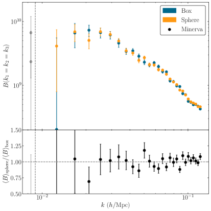
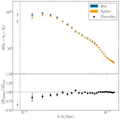
Figure 1: Top panels: mean of the bispectrum equilateral configurations, $\hat{B}_{0}(k,k,k)$, as a function of $k$ for both the box (blue) and spherical window (orange) measurements and for both the Minerva simulations (left) and Pinocchio box (right). Bottom panels: ratio of the sphere to box measurements for simulations and mocks. The vertical dashed line indicates the effective fundamental frequency of the sphere $k_{f}^{\mathrm{sphere}}=2\pi/V_{\rm sphere}^{1/3}$. The typical suppression induced by the window on large scales is only detectable in the case of the very large set of Pinocchio mocks.

The top panels of figure 1 show the mean of the measured bispectrum equilateral configurations, $\hat{B}_{0}(k,k,k)$, as a function of $k$ for both the box (blue) and spherical window (orange) and for both the Minerva simulations (left) and Pinocchio box (right). The bottom panels show the ratio of the sphere to box measurements for simulations and mocks. The typical suppression induced by the window on large scales is only detectable in the case of the very large set of mocks: for the even relatively large set of simulations ($\sim 1000\,h^{-3}\,{\rm Gpc}^{3}$ of total volume), the statistical errors are larger than any window effect. We stress, in this respect, that in the bispectrum case, where the signal is distributed over a large number of configurations, a systematic effect equally distributed over all configurations can have a sizable effect, even if small when compared to the statistical error for the single triangle.

In what follows we refer to the bispectrum monopole measurements $\hat{B}_{0}$ simply as $\hat{B}$, dropping the subscript for simplicity.

4.3 Theoretical model

The theoretical model that we adopt for the real-space bispectrum is the usual tree-level model in Standard Perturbation Theory (SPT), see e.g. [64] and [65, 66] for the inclusion of a term due to nonlocal bias. This is the same model already employed in [58] to whom we refer the reader for its detailed description and its fit to the same box bispectrum measurements considered here. We briefly summarise the full expression, given by

$$B(\mathbf{p}_{1},\mathbf{p}_{2})=b_{1}^{3}B_{\mathrm{TL}}(\mathbf{p}_{1},\mathbf{p}_{2})+b_{2}b_{1}^{2}\Sigma(\mathbf{p}_{1},\mathbf{p}_{2})+2b_{\mathcal{G}_{2}}b_{1}^{2}K(\mathbf{p}_{1},\mathbf{p}_{2})+B_{\mathrm{SN}}(\mathbf{p}_{1},\mathbf{p}_{2})\,,$$ (4.2)

where

$$B_{\mathrm{TL}}(\mathbf{p}_{1},\mathbf{p}_{2})=2F_{2}(\mathbf{p}_{1},\mathbf{p}_{2})P_{L}(p_{1})P_{L}(p_{2})+\mathrm{2~{}perms.}\,,$$ (4.3)

represents the tree-level matter bispectrum, $F_{2}$ being the standard quadratic PT kernel and $P_{L}(p)$ the linear matter power spectrum, while the quadratic local and nonlocal bias contributions are given by

$$\Sigma(\mathbf{p}_{1},\mathbf{p}_{2}) =P_{L}(p_{1})P_{L}(p_{2})+\mathrm{2~{}perms.}$$ (4.4)

$$K(\mathbf{p}_{1},\mathbf{p}_{2}) =\left[\left(\hat{p}_{1}\cdot\hat{p}_{2}\right)^{2}-1\right]P_{L}(p_{1})P_{L}(p_{2})+\mathrm{2~{}perms.}\,.$$ (4.5)

Finally, the shot-noise contribution is

$$B_{\mathrm{SN}}(\mathbf{p}_{1},\mathbf{p}_{2})=\frac{1}{\bar{n}}(1+\alpha_{1})b_{1}^{2}\left[P_{L}(p_{1})+P_{L}(p_{2})+P_{L}(p_{3})\right]+\frac{1}{\bar{n}^{2}}(1+\alpha_{2})\,,$$ (4.6)

with the $\alpha_{1}$ and $\alpha_{2}$ parameters allowing deviations from the Poisson prediction. We assume all cosmological parameters are known, thus the model depends only on five, free bias and shot-noise parameters: $b_{1}$, $b_{2}$, $b_{\mathcal{G}_{2}}$, $\alpha_{1}$ and $\alpha_{2}$.

4.4 Window convolution

Reducing eq. (3) to the case of the bispectrum monopole, i.e. $L=0$, and in real-space, $L^{\prime}=0$, $M^{\prime}=0$ in eq. (3), to describe the measurements of our test, gives the following expression for $\tilde{B}=\tilde{B}_{0}$

$$\tilde{B}(q_{1},q_{2},q_{3})=\int\frac{dp_{1}}{2\pi^{2}}p_{1}^{2}\int\frac{dp_{2}}{2\pi^{2}}p_{2}^{2}\int\frac{dp_{3}}{2\pi^{2}}p_{3}^{2}~{}B(p_{1},p_{2},p_{3})\sum_{\ell}I_{\ell\ell 0}(p_{1},p_{2},p_{3})\mathcal{Q}_{\ell}(q_{1},q_{2},q_{3};p_{1},p_{2}),$$ (4.7)

with

$$\mathcal{Q}_{\ell}(q_{1},q_{2},q_{3};p_{1},p_{2})\equiv\sum_{\ell^{\prime},\ell^{\prime\prime}}(2\ell^{\prime\prime}+1)(-1)^{\ell^{\prime\prime}}\begin{pmatrix}\ell&\ell^{\prime}&\ell^{\prime\prime}\\ 0&0&0\end{pmatrix}^{2}\mathcal{W}_{\ell\ell^{\prime}\ell^{\prime\prime}}(q_{1},q_{2};p_{1},p_{2}),$$ (4.8)

and

$$\mathcal{W}_{\ell\ell^{\prime}\ell^{\prime\prime}}(q_{1},q_{2};p_{1},p_{2})\equiv (4\pi)^{2}(2\ell+1)\int dx_{13}x_{13}^{2}\int dx_{23}x_{23}^{2}~{}j_{\ell}(p_{1}x_{13})j_{\ell}(p_{2}x_{23})$$

$$\times\Big{[}\mathcal{L}_{\ell^{\prime\prime}}(\hat{q}_{1}\cdot\hat{q}_{2})j_{\ell^{\prime\prime}}(q_{1}x_{13})j_{\ell^{\prime\prime}}(q_{2}x_{23})Q_{\ell^{\prime}}(x_{13},x_{23})\Big{]},$$ (4.9)

where $Q_{\ell}(x_{13},x_{23})$ is the 3PCF multipoles of the window function

$$Q_{\ell}(x_{13},x_{23})\equiv(2\ell+1)\int\frac{d^{2}\hat{x}_{13}}{4\pi}\int\frac{d^{2}\hat{x}_{23}}{4\pi}Q(\mathbf{x}_{13},\mathbf{x}_{23})\mathcal{L}_{\ell}(\hat{x}_{13}\cdot\hat{x}_{23}),$$ (4.10)

with

$$Q(\mathbf{x}_{13},\mathbf{x}_{23})\equiv\int d^{3}x_{3}~{}W(\mathbf{x}_{3})W(\mathbf{x}_{3}+\mathbf{x}_{13})W(\mathbf{x}_{3}+\mathbf{x}_{23}).$$ (4.11)

In addition to our approach to the convolution we also consider, for comparison, the approximation adopted in the analysis of [43, 44, 45] (see also [10, 28] for more recent work), which ignores the effect of the window convolution on the nonlinear kernel of the tree-level prediction while describing it in terms of a convolution of the power spectra. Symbolically we have

$$\tilde{B}[P_{L}]\simeq B[\tilde{P}_{L}]\,,$$ (4.12)

where $\tilde{P}_{L}(k)$ is the window convolution of the linear power spectrum, evaluated by the usual one-dimensional FFTLog method [33, 34, 37, 38]. This is given by

$$\tilde{P}(k)=\int\frac{dp}{2\pi^{2}}p^{2}~{}\mathcal{W}_{00}(k,p)P(p),$$ (4.13)

where $\mathcal{W}_{00}(k,p)$ is the mixing matrix

$$\mathcal{W}_{00}(k,p)\equiv 4\pi\int dx~{}x^{2}j_{0}(kx)j_{0}(px)Q(x),$$ (4.14)

with $Q(x)$ being the 2PCF of the window. We refer to this approach as “1DFFTLog approximation”. In this case the analysis is usually limited to those triangles where all sides are much larger than $1/R$, $R$ being the typical size of the window.

The two options described above apply to the tree-level bispectrum with the exception of the shot-noise contribution. The convolution of the latter is simply given by

$$\tilde{B}_{\mathrm{SN}}(\mathbf{p}_{1},\mathbf{p}_{2})=\frac{1}{\bar{n}}(1+\alpha_{1})b_{1}^{2}\left[\tilde{P}_{L}(p_{1})+\tilde{P}_{L}(p_{2})+\tilde{P}_{L}(p_{3})\right]+\frac{1}{\bar{n}^{2}}(1+\alpha_{2}),$$ (4.15)

where $\tilde{P}_{L}(p)$ is the window-convolved linear power spectrum, while we assume that the last constant term is not affected by the convolution.

As already mentioned, the ideal spherical geometry allows the window 3PCF to be evaluated analytically. The window function in configuration space can be written as

$$W(x)=\frac{1}{V^{1/3}}\theta(R-x),$$ (4.16)

where $R$ and $V$ are the radius and the volume of the sphere, respectively. The normalization is chosen such that the window 3PCF (4.11) is normalized to one for a uniform window function. The 3PCF multipoles $Q_{\ell}(x_{13},x_{23})$ of the window function, assuming $x_{13}<x_{23}$, have the following form

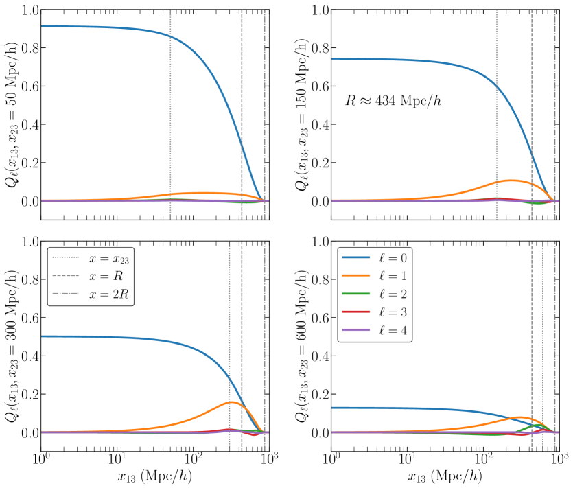
Figure 2: Spherical window 3PCF multipoles $Q_{\ell}(x_{13},x_{23})$ plotted as a function of $x_{13}$ at different, constant values of $x_{23}$. It is evident that the relative contribution of higher-order $Q_{\ell}$ becomes quickly less significant as $\ell$ increase.

$$Q_{\ell}\!=\!\begin{dcases}\left[\int_{0}^{R-x_{23}}dx_{3}x_{3}^{2}\int_{-1}^{1}\!\!\!\!d\mu_{1}\!\int_{-1}^{1}\!\!\!\!d\mu_{2}+\!\!\int_{R-x_{23}}^{R-x_{13}}dx_{3}x_{3}^{2}\int_{-1}^{1}\!\!\!\!d\mu_{1}\!\int_{-1}^{\mu_{2+}}d\mu_{2}+\!\!\int_{R-x_{13}}^{R}dx_{3}x_{3}^{2}\!\int_{-1}^{\mu_{1+}}\!\!\!\!d\mu_{1}\!\int_{-1}^{\mu_{2+}}\!\!\!\!d\mu_{2}\right]\int_{0}^{2\pi}\!\!\!\!\!\!d\phi\,G_{\ell}\\ \hskip 260.0004pt{\rm for}\quad x_{13}\leq x_{23}\leq R\,,\\ \left[\int_{x_{23}-R}^{R-x_{13}}dx_{3}x_{3}^{2}\!\int_{-1}^{1}\!\!\!\!d\mu_{1}\!\int_{-1}^{\mu_{2+}}\!\!\!\!d\mu_{2}+\int_{R-x_{13}}^{R}dx_{3}x_{3}^{2}\int_{-1}^{\mu_{1+}}\!\!\!\!d\mu_{1}\int_{-1}^{\mu_{2+}}\!\!\!\!d\mu_{2}\right]\int_{0}^{2\pi}\!\!\!\!d\phi\,G_{\ell}\\ \hskip 220.00034pt{\rm for}~{}x_{23}>R~{}\&~{}x_{13}+x_{23}\leq 2R\,,\\ \int_{x_{23}-R}^{R}dx_{3}x_{3}^{2}\int_{-1}^{\mu_{1+}}\!\!\!\!d\mu_{1}\int_{-1}^{\mu_{2+}}\!\!\!\!d\mu_{2}\int_{0}^{2\pi}\!\!\!\!d\phi\,G_{\ell}\hskip 83.00015pt{\rm for}~{}x_{23}>R~{}\&~{}x_{13}+x_{23}>2R\,,\\ 0\hskip 250.00038pt{\rm for}~{}x_{23}>2R\,,\end{dcases}$$ (4.17)

where

$$G_{\ell}(\mu_{1},\mu_{2},\phi)\equiv\frac{2\ell+1}{2V}\mathcal{L}_{\ell}\left[(1-\mu_{1}^{2})^{1/2}(1-\mu_{2}^{2})^{1/2}\cos\phi+\mu_{1}\mu_{2}\right]\,,$$ (4.18)

while

$$\mu_{1+}\equiv(R^{2}-x_{3}^{2}-x_{13}^{2})/(2x_{3}x_{13})\,,~{}~{}{\rm and}~{}~{}\mu_{2+}\equiv(R^{2}-x_{3}^{2}-x_{23}^{2})/(2x_{3}x_{23})\,.$$ (4.19)

Slices of the window 3PCF multipoles $Q_{\ell}(x_{13},x_{23})$, eq. (4.17), are shown in figure 2. Note that the lower-order multipoles dominate over the higher-order ones. In practice, as we will see later we only need to consider multipoles [$Q_{\ell}(x_{13},x_{23})$] up to $\ell^{\prime}=2$ (see also figure 8).

The details of the 2DFFTLog algorithm implementation are described in appendix A, where we show how variations with respect to the reference set-up only induce $\lesssim 2\%$ differences on the output. The two-dimensional Hankel transform that is required to compute (4.4) makes use of the public code 2DFFTLog [67]. We assume a bias $\nu(\ell)=1.1$, a window filter of width = 0.25, without additional extrapolation nor padding. For the 1DFFTLog approximation, we implement the one-dimensional Hankel transform in the mixing matrix of eq. (4.14) using the code mcfit with a sampling of 10000 log-spaced points from $p_{\mathrm{min}}=10^{-4}$ $h$/Mpc to $p_{\mathrm{max}}=1$ $h$/Mpc that is further constantly padded using end-point of both sides, up to $2^{15}$ number of points.

4.5 Binning effect

The measured $\hat{B}(k_{1},k_{2},k_{3})$ is the average over all fundamental triangles $\{\mathbf{q}_{1},\mathbf{q}_{2},\mathbf{q}_{3}\}$ that fall in the bins $q_{i}\in[k_{i}-\Delta k/2,k_{i}+\Delta k/2]$. Therefore our theoretical prediction for a given bin center $\{k_{1},k_{2},k_{3}\}$ should be binned in the same way.

In addition, a proper comparison with simulations should account as well for the discrete nature of Fourier-space wavenumbers, taking values $\mathbf{q}=\mathbf{n}k_{f}$, an aspect that, for simplicity, we have not explicitly included in our definition of the estimator, eq. (2.3).

A binning operator acting on some function $F(\mathbf{q}_{1},\mathbf{q}_{2},\mathbf{q}_{3})$ should therefore be written as

$$\Big{\langle}F(\mathbf{q}_{1},\mathbf{q}_{2},\mathbf{q}_{3})\Big{\rangle}_{\triangle}\equiv\frac{1}{N_{T}}\sum_{\mathbf{q}_{1}\in\mathbf{k}_{1}}\sum_{\mathbf{q}_{2}\in\mathbf{k}_{2}}\sum_{\mathbf{q}_{3}\in\mathbf{k}_{3}}F(\mathbf{q}_{1},\mathbf{q}_{2},\mathbf{q}_{3})\delta_{K}(\mathbf{q}_{123})\,,$$ (4.20)

where $N_{T}(k_{1},k_{2},k_{3})$ is the total number of “fundamental” triplets $\{\mathbf{q}_{1},\mathbf{q}_{2},\mathbf{q}_{3}\}$ satisfying the condition $\mathbf{q}_{123}=0$ enforced by the Kronecker symbol $\delta_{K}(\mathbf{q}_{123})$, that fall in the triangle bin $\{k_{1},k_{2},k_{3}\}$

$$N_{T}(k_{1},k_{2},k_{3})\equiv\sum_{\mathbf{q}_{1}\in\mathbf{k}_{1}}\sum_{\mathbf{q}_{2}\in\mathbf{k}_{2}}\sum_{\mathbf{q}_{3}\in\mathbf{k}_{3}}\delta_{K}(\mathbf{q}_{123})\,.$$ (4.21)

In the case of our 2DFFTLog approach, eq. (4.7), the effect of binning can be taken into account by applying such operator on the mixing matrix, eq. (4.4) as follows

$$\mathcal{W}_{\ell\ell^{\prime}\ell^{\prime\prime}}(k_{1},k_{2};p_{1},p_{2})\equiv (4\pi)^{2}(2\ell+1)\int dx_{13}x_{13}^{2}\int dx_{23}x_{23}^{2}~{}j_{\ell}(p_{1}x_{13})j_{\ell}(p_{2}x_{23})$$

$$\times\Big{[}\Big{\langle}\mathcal{L}_{\ell^{\prime\prime}}(\hat{q}_{1}\cdot\hat{q}_{2})j_{\ell^{\prime\prime}}(q_{1}x_{13})j_{\ell^{\prime\prime}}(q_{2}x_{23})\Big{\rangle}_{\triangle}Q_{\ell^{\prime}}(x_{13},x_{23})\Big{]}\,.$$ (4.22)

The high dimensionality of the matrix makes this procedure very expensive to compute exactly according to eq. (4.20). For this reason we consider two approximations explored already in [58, 59] (see also [68] and [15] for alternative approaches).

The first approximation amounts to simply evaluate our function

$$F(\mathbf{q}_{1},\mathbf{q}_{2},\mathbf{q}_{3})\equiv\mathcal{L}_{\ell}(\hat{q}_{1}\cdot\hat{q}_{2})j_{\ell}(q_{1}x_{13})j_{\ell}(q_{2}x_{23})$$ (4.23)

on the sorted, effective triplet $(\overline{k}_{1},\overline{k}_{2},\overline{k}_{3})$

$$\Big{\langle}F(q_{1},q_{2},q_{3})\Big{\rangle}_{\triangle}\simeq F(\overline{k}_{1},\overline{k}_{2},\overline{k}_{3}),$$ (4.24)

where

$$\overline{k}_{1} \equiv\Big{\langle}\mathrm{max}\{q_{1},q_{2},q_{3}\}\Big{\rangle}_{\triangle},$$

$$\overline{k}_{2} \equiv\Big{\langle}\mathrm{med}\{q_{1},q_{2},q_{3}\}\Big{\rangle}_{\triangle},$$ (4.25)

$$\overline{k}_{3} \equiv\Big{\langle}\mathrm{min}\{q_{1},q_{2},q_{3}\}\Big{\rangle}_{\triangle},$$

such that $\mathrm{max}\{q_{1},q_{2},q_{3}\}\geq\mathrm{med}\{q_{1},q_{2},q_{3}\}\geq\mathrm{min}\{q_{1},q_{2},q_{3}\}$. A better approximation can be obtained including higher-order corrections in a Taylor-expansion about the effective wavenumbers [59]. This corresponds to

$$\Big{\langle}F(q_{1},q_{2},q_{3})\Big{\rangle}_{\triangle}\simeq F(\overline{k}_{1},\overline{k}_{2},\overline{k}_{3})+\frac{1}{2}\sum_{i,j}\frac{\partial^{2}}{\partial q_{i}\partial q_{j}}F(\overline{k}_{1},\overline{k}_{2},\overline{k}_{3})\Big{\langle}(q_{i}-\overline{k}_{i})(q_{j}-\overline{k}_{j})\Big{\rangle}_{\triangle}.$$ (4.26)

On the other hand, the binning of the prediction in the 1DFFTLog approximation approach is closer to the procedure in [59] for the unconvolved bispectrum. For a generic tree-level expression such as $B(q_{1},q_{2},q_{3})=K(\mathbf{q}_{1},\mathbf{q}_{2})P_{L}(q_{1})P_{L}(q_{1})+{\rm perm.}$, we evaluate the Taylor expansion around the $\overline{k}_{i}$ as

$$\Big{\langle}\tilde{B}(q_{1},q_{2},q_{3})\Big{\rangle}_{\triangle}\simeq\sum_{n+m\leq 2}\frac{1}{n!m!}\Big{\langle}K(\mathbf{q}_{1},\mathbf{q}_{2})(q_{1}-\overline{k}_{1})^{n}(q_{2}-\overline{k}_{2})^{m}\Big{\rangle}_{\triangle}\tilde{P}^{(n)}_{L}(\overline{k}_{1})\tilde{P}^{(m)}_{L}(\overline{k}_{2})+\mathrm{perm.}\,,$$ (4.27)

where $\tilde{P}^{(n)}_{L}$ is the $n$-derivative of the convolved linear power spectrum. The $n=m=0$ term represent the leading contribution, corresponding to the first approximation of eq. (4.24).

4.6 Likelihood analysis and covariance

In the next section we test our convolution expression against measurements both from the Minerva simulations and from the Pinocchio mocks. In both cases, the theoretical prediction is evaluated as the posterior-averaged convolved tree-level model by performing a likelihood analysis in terms of the five bias and shot-noise parameters, fixing the cosmological parameters. This consists in practice in averaging the model over the corresponding Markov chains.

We consider a total log-likelihood function given by the sum of the log-likelihood of each individual realisation, so that

$$\ln{\mathcal{L}}_{\rm tot}=\sum_{\alpha=1}^{N_{R}}\ln{\mathcal{L}}_{\rm\alpha}\,,$$ (4.28)

where $N_{R}$ is the total number of realisations of either mocks or simulations. For the single realisation we assume a Gaussian likelihood defined as

$$\ln\mathcal{L}_{\alpha}=-\frac{1}{2}\sum_{i,j}\Delta B_{i}C_{ij}^{-1}\Delta B_{j},$$ (4.29)

where $i$ is the triangle index, $\Delta B_{i}=\hat{B}_{i}^{(\alpha)}-\tilde{B}_{i}$ is the difference between the measurement and theoretical prediction, while $C_{ij}$ is the bispectrum covariance matrix estimated numerically from the $10000$ Pinocchio mocks measurements. The large number of mocks provides a robust estimates of the covariance were residual statistical errors can be ignored [58].

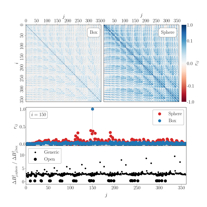
Figure 3: The cross-correlation matrix $r_{ij}$ for $\Delta k=2\,k_{f}$ bin size, estimated from 10000 Pinocchio mocks. Mode-coupling from the window-bispectrum convolution induced a significant contribution from the non-diagonal term in the correlation matrix of the sphere data. The middle panel highlights the elements of $r_{ij}$ corresponding to the $i=150$ triangle. The bottom panel shows the ratio of the variance $\Delta B^{2}_{i}\equiv C_{ii}$ from the sphere and box catalogs. Leakage to the non-diagonal elements is the possible cause for this ratio to be less than the factor expected from the volume ratio $\sim(1500/700)^{3}$ between the sphere and the box. In particular, the effect is most severe for some of the open configurations, where the ratio of the variance is in the minimum. It is also interesting to note that the maximum of the ratio is happened to be in the squeezed configurations.

The cross-correlation matrix, defined as

$$r_{ij}\equiv\frac{C_{ij}}{\sqrt{C_{ii}C_{jj}}}\,,$$ (4.30)

estimated from the spherical window measurements is shown in figure 3 (top right panel), where it is compared to the analogous quantity corresponding to the box measurements (top left panel). The correlation among different modes induced by the window results clearly in larger off-diagonal elements. The middle panel of figure 3 shows the elements of $r_{ij}$ corresponding to the $i=150$ triangle, as a function of $j$, while the bottom panel hows the ratio of the variance $\Delta B^{2}_{i}\equiv C_{ii}$ from the sphere and box catalogs. Leakage to the non-diagonal elements likely causes this ratio to be less than the factor one could naively expect from the volume ratio $\sim(1500/700)^{3}$ between the sphere and the box.

We perform the analysis by means of MCMC (Monte Carlo Markov Chain) simulations using the Python implementation of affine-invariant ensemble sampler emcee [69]. Initially, the linear power spectrum is obtained from the CAMB code [70] assuming the fiducial cosmology. Each run of the chain, the bias parameter space is explored using 100 walkers. The chain is assumed to be converged after the number of steps is larger than 100 times integrated autocorrelation time $\tau$[71]. All the ingredients required to perform this analysis are compiled in the modified PBJ (P+B Joint analysis) code [58, 59], which we now extended to include the window-convolved bispectrum prediction. Note that in the case of fixed cosmology, the window-convolution process only need to be done once, since the bias parameters can be factored-out. Nevertheless, as we show in figure 10 of appendix B, each evaluation of the convolved bispectrum is comparable with a typical call of the Boltzmann solver. More precisely, for bin size $\Delta k=2\,k_{f}$ with the total number of triangles $N_{T}=360$, using as default parameters those described in appendix B, the evaluation of the tree-level model and the matrix multiplication take each $\sim 1$ seconds.

In all our fits, the free parameters are $\{b_{1},b_{2},b_{\mathcal{G}_{2}},\alpha_{1},\alpha_{2}\}$ with the priors given in table 1.

Parameters	Priors (uniform)
$b_{1}$	[0.9, 3.5]
$b_{2}$	[-4, 4]
$b_{\mathcal{G}2}$	[-5, 5]
$\alpha_{1}$	[-1, 1]
$\alpha_{2}$	[-1, 1]

Table 1: Prior assumed for the bias and shot-noise parameters in all likelihood evaluations.

5 Results

5.1 Comparison with mocks measurements

In this section we compare the prediction of the 2DFFTLog-based approach and the approximation using 1DFFTLog to the average of bispectrum measurements from the full set of Pinocchio mocks. This extremely large set of measurements allows to keep the statistical noise below the systematic errors under investigation.

Theoretical predictions are defined as the posterior-averaged bispectrum $\langle\tilde{B}(k_{1},k_{2},k_{3})\rangle_{\rm post}$ from the likelihood analysis of the 10000 Pinocchio box mocks including all triangles up to $k_{\mathrm{max}}=0.09\,h\,{\rm Mpc}^{-1}$, using the same data-set to estimate the covariance. Nota bene: all theoretical predictions in this section, either for box or sphere measurements, are averaged over the same Markov chain corresponding to the likelihood analysis of the box measurements: this ensures that differences induced by systematic errors on the convolution are not reduced by fitting the free parameters. In other terms, we are comparing the different convolution methods adopting the model parameters determined, in both cases, from the analysis of the mocks bispectrum measured in the box according to the likelihood of eq’s (4.28) and (4.29).

The prediction for the unconvolved bispectrum is binned using the exact expression of eq. (4.20) (see also [58]), while the convolved prediction for both 2DFFTLog and 1DFFTLog approximation adopts the expansion method of eq. (4.26) and eq. (4.27), respectively. We have checked on a limited subset of configurations that even in the convolved bispectrum case, the difference between the expansion and the exact binning is below 0.5%, more than an order of magnitude smaller than the effect of the window.

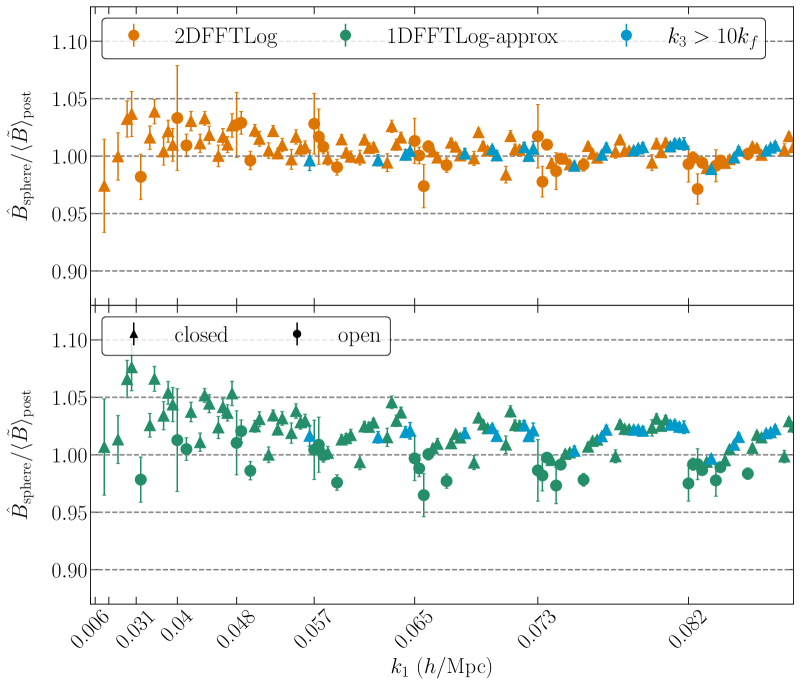
Figure 4: Ratio of the average of the bispectrum measurements from the 10000 Pinocchio mocks for all configurations (up to $k_{1}\leq 0.09$ $h$/Mpc) to the theoretical prediction of the 2DFFTLog method (top panel) and the 1DFFTlog approximation (bottom panel). Both predictions are the posterior-averaged bispectrum $\langle\tilde{B}(k_{1},k_{2},k_{3})\rangle_{\rm post}$ from the likelihood analysis of the box measurements of the 10000 Pinocchio mocks with $k_{\mathrm{max}}=0.09\,h\,{\rm Mpc}^{-1}$ using the same data-set to estimate the covariance. The error bar is the error on the mean from the mocks. We mark in blue the configurations with the smallest wavenumber $k_{3}>10k_{f}$, in general showing a better agreement.

Figure 4 shows the ratio of the measurements to the convolved model for all configurations up to $k_{\rm max}=0.09\,h\,{\rm Mpc}^{-1}$, with the top panel corresponding to the 2DFFTlog approach and the bottom panel to the 1DFFTlog approximation. The error bars correspond to the error on the mean of ratios of the 10000 Pinocchio data and the prediction. The 2DFFTLog based method matches the data fairly well with $\lesssim 2-3\%$ errors and a marginal, residual dependence on shape. The discrepancy becomes slightly worse on large scales but is still within $\lesssim 5\%$ error level. Here we observe a scatter among the very first points slightly larger then the estimated error bars. This could be due to finite density of the random catalog adopted in the bispectrum estimator and to the fact that a single random has been used for all measurements.

In the case of the 1DFFTLog approximation we notice differences with the measurements up to 6-7% and a similar but larger shape-dependence. We also notice that at large scale, in addition to the scatter mentioned above, it tends to underestimate the usual suppression of power. It should be noted, on the other hand, that the 1D approximation fares relatively well, despite the crude simplification.

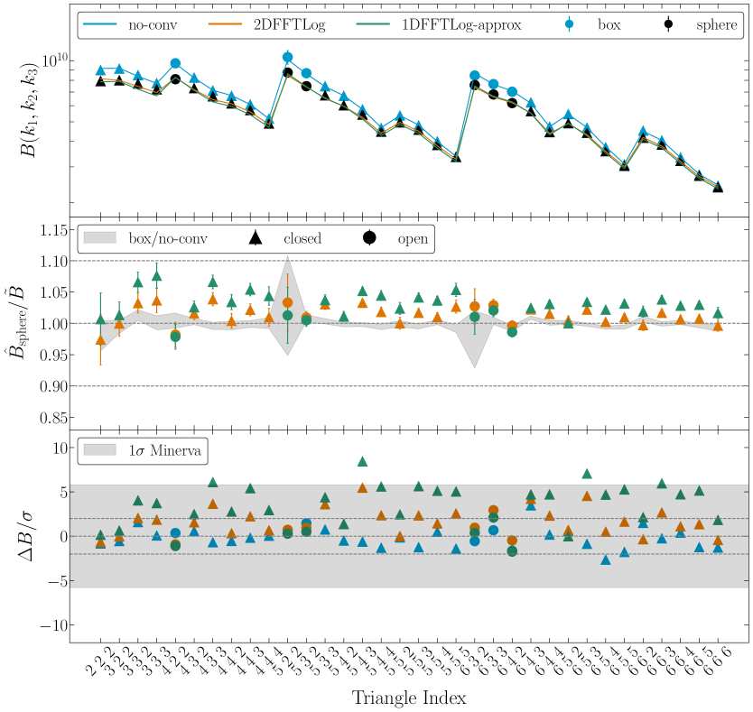
Figure 5: Comparison between the theoretical prediction on the first 34 triangles of Pinocchio box/sphere for $s=2$ bin size. All theoretical predictions are the posterior-averaged bispectrum from the likelihood analysis of the 10000 Pinocchio box mocks with $k_{\mathrm{max}}=0.09\,h\,{\rm Mpc}^{-1}$ using the same data-set to estimate the covariance. The 2DFFTLog method match the data on the level of uncertainty present in the unconvolved prediction (mostly within 2$\sigma$ away with some outliers which still within 5$\sigma$). All theoretical prediction agree with the data within 1$\sigma$ corresponding to Minerva volume.

In figure 4 we also singled-out, as blue points, those triangles where all sides are larger than $10k_{f}\approx 0.04\,h\,{\rm Mpc}^{-1}$. This is approximately equivalent to the triangles selected for the analysis of [43, 44], where the 1DFFTLog method is applied. The motivation was to exclude the configurations where the effect of the window is not properly accounted for by the 1D approximation. Indeed, this appears to be the case in our spherical, ideal case, with lower systematic errors and smaller dependence on scale.

In figure 5 we zoom-in to the first 34 triangles, roughly up to largest side of the triangles $k_{1}\approx 0.05\,h\,{\rm Mpc}^{-1}$. The top panel shows the measurements and the predictions, both in the box and the sphere. The middle panel shows the ratio between Pinocchio mocks, sphere measurements and the corresponding predictions, with the gray band corresponding to the same ratio for the box/unconvolved case. This shows that part of the scatter and to some extent, the shape-dependent systematic error is also present in the box comparison and it is therefore not due to the convolution. We see as well that the 2DFFTLog method matches the data fairly well, at the level of uncertainty present in the box case. The 1DFFTLog approximation is $\sim$ (1-2)$\sigma$ worse than the 2DFFTLog and is consistently underpredicting the data. In the third panel we show the relative error with respect to the variance of the 10000 Pinocchio mocks. The 2DFFTLog prediction is mostly within 2$\sigma$ (comparable with the unconvolved prediction) with some outliers still within 5$\sigma$. The panel also shows as a gray band the 1-$\sigma$ uncertainty corresponding to the measurements from the set of Minerva simulations, that we will consider in the next section.

In the end, in our test, we see that window effect on the bispectrum is a very tiny effect mainly on large scales which can be only probed by using a very large number of realisations. We notice that the 1DFFTlog approximation fares rather well, with a small overall offset that does not present a marked dependence on shape, at least in our spherical, ideal case in real-space. Still, we will study how such off-set, present with the same size and sign on all configurations, could affect the analysis of data sets even of much smaller cumulative volumes than the extreme case considered here.

5.2 Recovering bias parameters from the N-body measurements

We consider now independent fits to the N-body simulations of the theoretical model with each of the convolution methods in order to asses their effect on the recovered bias parameters. Again we fit individually all distinct realisations according to the likelihood function described in eq.s (4.28) and (4.29).

The sphere measurements from the 298 Minerva simulations correspond to a more realistic test since the total volume, of about $100\,h^{-3}\,{\rm Gpc}^{3}$, is roughly 1/4 of the blinded challenge volume presented in [72] and approximately 10 times the volume of the largest redshift bin of Euclid survey considered in the forecasts of [73]. As it can be seen from the bottom panel of figure 5, both unconvolved and window-convolved prediction agree with the data within 1$\sigma$ of the Minerva measurements. Still, a small systematic effect distributed over a large number of data-points can affect the determination of cosmological parameters.

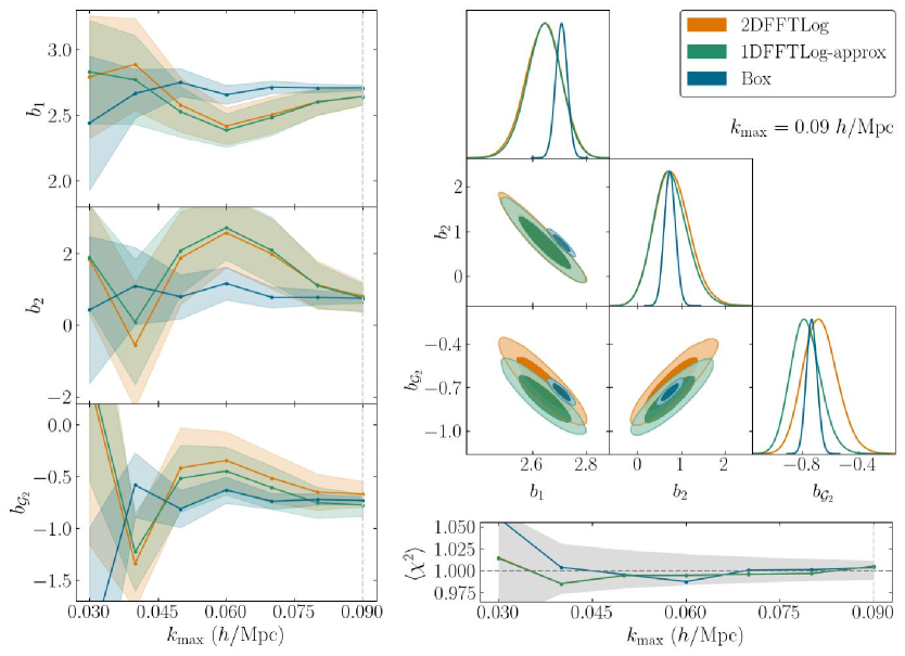
Figure 6: Left panels: marginalised 1-$\sigma$ constraints on the bias parameters as a function of $k_{\rm max}$ from the box measurements analysis (blue) and from the sphere measurements assuming the 2DFFTlog (orange) and 1DFFTlog approximation (green) predictions. Top-right panel: marginalised 2-parameters contours at $k_{\rm max}=0.09\,h\,{\rm Mpc}^{-1}$. Bottom-left panel: posterior-averaged, reduced $\chi^{2}$ as a function of $k_{\rm max}$, with the gray band marking the 95% C.L. interval.

The posteriors for the bias parameters are shown in figure 6. The figure provides the 1-$\sigma$ constraints as a function of the largest side of the triangle on the left panels while the top-right panel shows the marginalised 2-parameters contours at $k_{\rm max}=0.09\,h\,{\rm Mpc}^{-1}$. Finally, the bottom-left shows the posterior-averaged, reduced $\chi^{2}$ as a function of $k_{\rm max}$, compared with the 95% C.L. interval shown as a gray band. The larger constraints from the Minerva sphere analysis with respect to the Minerva box analysis are simply due to the difference in volume, which a ratio of roughly a factor of 8. All constraints are marginalised over the shot-noise parameters that we are not showing for clarity.

We can see that bias parameter recovered from Minerva box and sphere analysis (for both methods) agree within 1$\sigma$. This level agreement is expected since as we have shown in the previous section, sample variance dominates over window effects on large scales. Yet, in the contour plots one can notice a purely systematic effect almost at the 2-$\sigma$ level between the two convolution methods that could become more relevant at smaller scales, where the model should be extended to include loop corrections.

We derived all the results presented in this section assuming a different, smaller bin size ($\Delta k=k_{f}$) for the wavenumber in all bispectrum measurements. Since we do not observe any relevant difference in our conclusions we do not include them in this presentation.

6 Conclusions

In this work we laid out an expression for the exact convolution with a survey window function for the redshift-space bispectrum multipoles as defined in [31]. The window convolution we propose is based on a two-dimensional Hankel transform implemented by means of the 2DFFTlog code of [67], an extension of the 1D FFTlog algorithm by [40]. Our implementation allows for an efficient computation, via FFTs, of the mixing matrix relating theoretical predictions to the corresponding observable by means of a matrix multiplication. The mixing matrix has to be computed only once and it is provided as input to the likelihood analysis. The multiplication of the theory bispectrum with the mixing matrix, in the case of total number of triangles $N_{T}=360$, takes $\sim 1$ seconds which is comparable to running time of a typical call to a Boltzmann solver. On the other hand our approach provides an improvement over the 1D approximation adopted in [43, 44, 45, 10, 28] and should provide a benchmark for alternative bispectrum estimators such as those of [47] and [50].

We test our expression in the ideal setting of a spherical window function where the 3-point correlation function of the footprint can be computed analytically. We compare our prediction for the convolved bispectrum monopole in real space to the average of measurements from halo mock catalogs. The average is taken from an extremely large number of realizations, in order to keep the statistical noise below the systematic errors under consideration. We notice that, at least in this example, the effect of the window is quite small. Nevertheless, our 2DFFTlog approach reduces significantly the errors characterising the 1D approximation, with residuals at the few-percent level and weak dependence on shape. Always within the spherical window model, we then explored the effect of the two methods on the determination of the bias (and shot-noise) parameters from the halo catalogs of the Minerva simulations for a total volume of about 100$\,h^{-3}\,{\rm Gpc}^{3}$. We find differences in the determination of the linear and nonlocal bias parameters at the 2-$\sigma$ level, suggesting the need of further investigations in a more realistic context.

The results of this preliminary comparison might quantitatively change in more realistic setups. For instance, the effect of the window will be more evident for higher multipoles in redshift-space and for models with a specific signal in squeezed configuration such as local primordial non-Gaussianity or relativistic effects [74, 24, 75, 76, 77, 78, 25, 79, 80, 26]. Also, while the overall window effect should decrease at small scales ($k\gtrsim 0.1\,h\,{\rm Mpc}^{-1}$), the 1D approximation is expected to fail when loop corrections become important: in this respect, again, squeezed configuration might require particular attention. Finally, the 1D approximation does not take into account the coupling of different bispectrum multipoles induced by window function effects.

We will explore in future work more realistic scenarios. Here, we limit ourselves to observe that the implementation of the multiplication by the window matrix introduced here does not significantly changes the run-time for a typical Markov chain and could therefore provide a safer, more robust approach to the bispectrum convolution for the bispectrum multipole estimator of [31].

Appendix A Convergence tests and binning systematics

The evaluation of the mixing matrix underlying all the results presented in the main text adopts a set of default values for several parameters. We explore in section A.1 how our results depend on their choice, while in section A.2 we quantify the systematic error related to the binning scheme.

A.1 2DFFTLog parameters

The first relevant parameter in the 2DFFTlog evaluation of eq. (3) is the number of sampling points $N_{p}$ for the linear power spectrum. The prediction for the unconvolved bispectrum is evaluated for all (closed) triangles one can form based on the $N_{p}$ wavenumber values, so that one of the dimension of the mixing matrix scales like $N_{p}^{3}$. We assume as default value $N_{p}=512$. Other two parameters are the maximum values for the multipoles $\ell$ and $\ell^{\prime}$, for which we take as default $\ell_{\mathrm{max}}=30$ and $\ell^{\prime}_{\mathrm{max}}=2$. We have then the range of integration over $p$, with $\{p_{\rm min},p_{\rm max}\}=\{10^{-5},0.5\}\,h\,{\rm Mpc}^{-1}$ as reference.

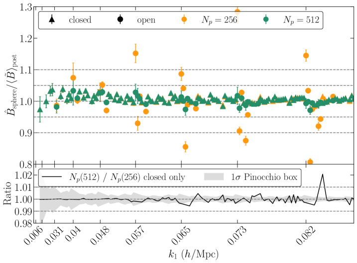
Figure 7: Top panel: the effect of varying the number of sampling points $N_{p}$ in the comparison of measurements to the theoretical prediction evaluated for $N_{p}=512$ (the default value, green) and $N_{p}=256$ (yellow). “Open” triangles are shown with circle markers while regular, “closed” triangles are shown with triangles. Bottom panel: ratio of the two predictions compared to the 1-$\sigma$ error on the mean of the Pinocchio measurements.

The effect of varying the number of sampling points $N_{p}$ (fixing the other parameters to their default values) is shown in figure 7. Interestingly enough, reducing $N_{p}$ into $256$ affects significantly the open configurations, while it only gives a $\leq 2\%$ difference on regular, closed triangles. Reducing $N_{p}$ has the advantage of reducing the mixing matrix generation time significantly (see table 2) while also reducing the time required by the matrix multiplication (see figure 10). A practical approach could be an hybrid method where the 1DFFTLog approximation handles the open configurations while the 2DFFTLog is used for the rest.

Figure 8 shows the effects of varying the other four parameters $\ell_{\rm max}$, $\ell^{\prime}_{\rm max}$, $p_{\rm min}$ and $p_{\rm max}$, in terms of ratios with the default evaluation of the prediction. Varying $p_{\mathrm{min}}$ and $p_{\mathrm{max}}$ is done in such a way that the spacing $\Delta\ln p$ is fixed. The variation of all these parameters only induce $\lesssim 2\%$ difference with respect to the default case except for $p_{\mathrm{max}}=0.2\,h\,{\rm Mpc}^{-1}$ which apparently is too low for our data vector extending to $k_{\mathrm{max}}\approx 0.09$ $h$/Mpc.

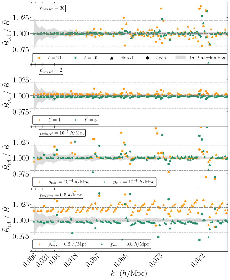
Figure 8: Ratio of the reference prediction for the convolved bispectrum w.r.t. the same prediction computed with different choices for the parameters $\ell_{\rm max}$, $\ell^{\prime}_{\rm max}$, $p_{\rm min}$ and $p_{\rm max}$.

A.2 Binning effects

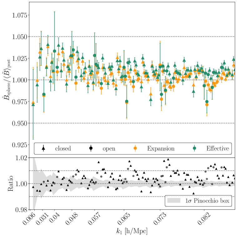
Figure 9: Comparison between the simpler effective binning of eq. (4.24) with expansion binning of eq. (4.26) for $\Delta k=2\,k_{f}$ bin size. The difference is only at $\lesssim 2\%$ level.

In figure 9, we compare the simpler effective binning of eq. (4.24) with the Taylor expansion defined in eq. (4.26), which is used for all our results in the main text. The effect of binning for the window-convolved bispectrum is at the $\lesssim 2\%$ level, which is smaller than effect of binning on the typical unconvolved bispectrum [58]. The advantage of the effective binning is again that it speeds up the computation of the mixing matrix (see table 2). As an additional check, we also computed the exact binning procedure of eq. (4.5) for a limited set of representative triangular configurations. We found that the difference with the Taylor expansion approach is below $0.5\%$ for all triangles considered.

Appendix B Memory and time requirement

In this appendix we describe the performance of the Python implementation of the 2DFFTLog method for the bispectrum convolution in our test of a real-space, spherical window function. In table 2 we compare the time and memory requirement to generate the mixing matrix, for the two binning methods of eq.s  (4.24) and (4.26) and for different values of the number of sampling points $N_{p}$. In general, the expansion method take a factor 2 or 3 more time to generate the mixing matrix, while requiring approximately the same amount of memory. The time required as a function of $N_{p}$ is also shown in figure 10. The initialization of each chain in a MCMC run, which consists of generating the triangles $\{p_{1},p_{2},p_{3}\}$ in log-space and loading the mixing matrix $\mathcal{M}$, takes few minutes. At each sampling of the parameter space that requires a call for the linear power spectrum, the unconvolved bispectrum has to be evaluated on the triangles $\{p_{1},p_{2},p_{3}\}$ and then multiplied with the mixing matrix. Both processes separately take $\sim$ 1 second for $N_{p}\sim 500$. The time taken by the matrix multiplication also depends linearly, as one can expect, on the number of redshift-space multiples considered and on the number of triangles $N_{T}$, which can be reduced by choosing a larger bin size $\Delta k$.

$\Delta k=2\,k_{f}$,  $N_{T}=360$
Binning method	$N_{p}$	Memory (GB)	Time (hrs:mins)
Effective	512	29.85	02:01
	256	6.55	00:15
Expansion	512	30.08	04:02
	256	7.02	00:45

Table 2: Comparison of memory and time required to generate the mixing matrix for different binning methods and different values of the number of sampling points $N_{p}$.

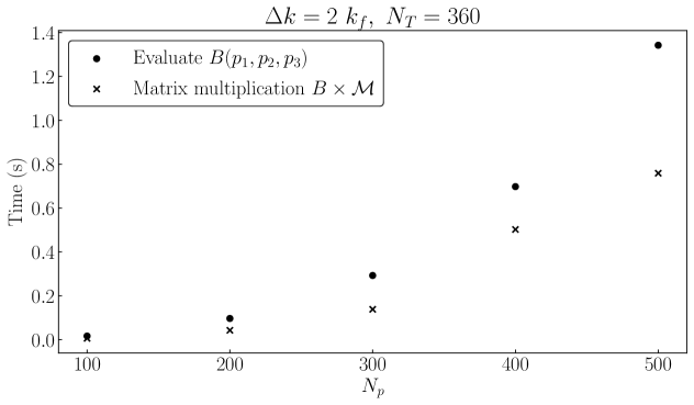
Figure 10: Time required for the matrix multiplication compared to the evaluation of the unconvolved bispectrum $B(p_{1},p_{2},p_{3})$ as a function of the number of sampled points $N_{p}$. In all cases the number of measured triangles is kept fixed at $N_{T}=360$.

Appendix C On the measurement of the window 3PCF multipoles

We are not addressing in this work the problem of the optimal estimator for the window 3PCF multipoles $Q^{L}_{L^{\prime}M^{\prime}\ell\ell^{\prime}\ell_{1}\ell_{2}}(x_{13},x_{23})$ defined in eq. (3), and of the systematic errors related to their measurement. We simply notice that in addition to direct pair-counting, one could consider an FFT-based estimator, since [49]

$$Q^{L}_{L^{\prime}M^{\prime}\ell\ell^{\prime}\ell_{1}\ell_{2}}(x_{13},x_{23})=\, (-1)^{M^{\prime}}\sum_{\begin{subarray}{c}M,m_{1},m_{2}\\ m,m^{\prime}\end{subarray}}\sum_{\begin{subarray}{c}\tilde{\ell}_{1},\tilde{\ell}_{2}\\ \tilde{m}_{1},\tilde{m}_{2}\end{subarray}}4\pi i^{\ell^{\prime}-\ell+\ell_{2}-\ell_{1}}~{}\mathcal{G}_{L\ell_{1}\ell_{2}}^{Mm_{1}m_{2}}\mathcal{G}_{L^{\prime}\ell\ell^{\prime}}^{M^{\prime}mm^{\prime}}\mathcal{G}_{\tilde{\ell}_{1}\ell_{1}\ell^{\prime}}^{\tilde{m}_{1}m_{1}m^{\prime}}\mathcal{G}_{\tilde{\ell}_{2}\ell_{2}\ell}^{\tilde{m}_{2}m_{2}m}$$

$$\times\int~{}d^{3}x_{3}~{}W_{\tilde{\ell}_{1}\tilde{m}_{1}}(\mathbf{x}_{3};x_{13})W_{\tilde{\ell}_{2}\tilde{m}_{2}}(\mathbf{x}_{3};x_{23})W_{LM}(\mathbf{x}_{3})\,,$$ (C.1)

can be obtained in terms of the Fourier Transform

$$W_{\ell m}(\mathbf{x}_{3};x_{ij})\equiv\,i^{\ell}\int\frac{d^{3}q}{(2\pi)^{3}}e^{i\mathbf{q}\cdot\mathbf{x}_{3}}j_{\ell}(qx_{ij})Y_{\ell m}(\hat{q})W(\mathbf{q})\,,$$ (C.2)

and

$$W_{LM}(\mathbf{x}_{3})\equiv\,W(\mathbf{x_{3}})Y^{*}_{LM}(\mathbf{x}_{3})\,.$$ (C.3)

The window 3PCF can also be expanded in TripoSH basis with zero total angular momentum, as follows [47]

$$Q(\mathbf{x}_{13},\mathbf{x}_{23},\hat{x}_{3})=\sum_{\ell_{1},\ell_{2},L}Q_{\ell_{1}\ell_{2}L}(x_{13},x_{23})\times \Bigg{[}\sqrt{\frac{4\pi}{(2\ell_{1}+1)(2\ell_{2}+1)(2L+1)}}\begin{pmatrix}\ell_{1}&\ell_{2}&L\\ 0&0&0\end{pmatrix}^{-2}$$

$$\,\,\sum_{m_{1},m_{2},M}\mathcal{G}_{\ell_{1}\ell_{2}L}^{m_{1}m_{2}M}Y_{\ell_{1}m_{1}}(\hat{x}_{13})Y_{\ell_{2}m_{2}}(\hat{x}_{23})Y_{LM}(\hat{x}_{3})\Bigg{]}.$$ (C.4)

The window 3PCF multipoles, eq. (3), are then related to the $Q_{\ell_{1}\ell_{2}L}(x_{13},x_{23})$, via the following linear combination

$$Q^{L}_{L^{\prime}M^{\prime}\ell\ell^{\prime}\ell_{1}\ell_{2}}(x_{13},x_{23})=\sum_{\tilde{\ell}_{1},\tilde{\ell_{2}}}Q_{\tilde{\ell}_{1}\tilde{\ell}_{2}L}(x_{13},x_{23})\,\mathbb{M}_{\tilde{\ell}_{1}\tilde{\ell}_{2}L;L^{\prime}M^{\prime}\ell\ell^{\prime}\ell_{1}\ell_{2}},$$ (C.5)

where

$$\mathbb{M}_{\tilde{\ell}_{1}\tilde{\ell}_{2}L;L^{\prime}M^{\prime}\ell\ell^{\prime}\ell_{1}\ell_{2}}\equiv \sum_{\begin{subarray}{c}M,m_{1},m_{2}\\ m,m^{\prime},\tilde{m}_{1},\tilde{m}_{2}\end{subarray}}(-1)^{M+\tilde{m}_{1}+\tilde{m}_{2}}\,i^{\ell^{\prime}-\ell+\ell_{2}-\ell_{1}}\sqrt{\frac{(4\pi)^{3}}{(2\tilde{\ell}_{1}+1)(2\tilde{\ell}_{2}+1)(2L+1)}}$$

$$\times\begin{pmatrix}\tilde{\ell}_{1}&\tilde{\ell}_{2}&L\\ 0&0&0\end{pmatrix}^{-2}\,\mathcal{G}_{L\ell_{1}\ell_{2}}^{Mm_{1}m_{2}}\,\mathcal{G}_{L\tilde{\ell}_{1}\tilde{\ell}_{2}}^{M-\tilde{m}_{1}-\tilde{m}_{2}}\,\mathcal{G}_{L^{\prime}\ell\ell^{\prime}}^{M^{\prime}mm^{\prime}}\,\mathcal{G}_{\ell_{1}\ell^{\prime}\tilde{\ell}_{1}}^{m_{1}m^{\prime}\tilde{m}_{1}}\,\mathcal{G}_{\ell_{2}\ell\tilde{\ell}_{2}}^{m_{2}m\tilde{m}_{2}}\,.$$ (C.6)

Written this way, the corresponding window bispectrum multipoles $B_{W,\ell_{1}\ell_{2}L}(k_{1},k_{2})$, which are related to $Q_{\ell_{1}\ell_{2}L}(x_{13},x_{23})$ through a double Hankel transform [47], can also be used as an input measurements.

Appendix D Useful identities

In this appendix we collect several well-known mathematical identities employed in the derivation of the main results in section 3. Our convention for the spherical harmonics is such that

$$Y_{\ell 0}(\theta,\phi)=\sqrt{(2\ell+1)/4\pi}~{}\mathcal{L}_{\ell}(\theta)\,,$$ (D.1)

where $\mathcal{L}_{\ell}(\theta)$ is Legendre polynomial of order $\ell$.

Rayleigh expansion of a plane wave:

$$e^{i\mathbf{k}\cdot\mathbf{x}}=\sum_{\ell}i^{\ell}(2\ell+1)j_{\ell}(kx)\mathcal{L}_{\ell}(\hat{k}\cdot\hat{x})\,.$$ (D.2)

Addition of spherical harmonics:

$$\mathcal{L}_{\ell}(\hat{x}\cdot\hat{y})=\frac{4\pi}{2\ell+1}\sum_{m}Y_{\ell m}(\hat{x})Y_{\ell m}^{*}(\hat{y})\,.$$ (D.3)

Orthogonality of Legendre polynomials:

$$(2\ell+1)\int\frac{d^{2}\hat{k}}{4\pi}\mathcal{L}_{\ell}(\hat{k}\cdot\hat{x})\mathcal{L}_{\ell^{\prime}}(\hat{k}\cdot\hat{y})=\delta_{\ell\ell^{\prime}}\mathcal{L}_{\ell}(\hat{x}\cdot\hat{y})\,$$ (D.4)

which implies that

$$\int\frac{d^{2}\hat{k}}{4\pi}e^{i\mathbf{k}\cdot\mathbf{x}}\mathcal{L}_{\ell}(\hat{k}\cdot\hat{y})=i^{\ell}j_{\ell}(kx)\mathcal{L}_{\ell}(\hat{x}\cdot\hat{y})\,.$$ (D.5)

Orthogonality of spherical harmonics:

$$\int d^{2}\hat{k}~{}Y_{\ell m}(\hat{k})Y^{*}_{\ell^{\prime}m^{\prime}}(\hat{k})=\delta_{\ell\ell^{\prime}}\delta_{mm^{\prime}}\,.$$ (D.6)

which implies that

$$\int\frac{d^{2}\hat{k}}{4\pi}e^{i\mathbf{k}\cdot\mathbf{x}}Y_{\ell m}(\hat{k})=i^{\ell}j_{\ell}(kx)Y_{\ell m}(\hat{y})\,.$$ (D.7)

Gaunt’s integral:

$$\int d^{2}\hat{k}~{}Y_{\ell_{1}m_{1}}(\hat{k})Y_{\ell_{2}m_{2}}(\hat{k})Y_{\ell_{3}m_{3}}(\hat{k})=\mathcal{G}^{m_{1}m_{2}m_{3}}_{\ell_{1}\ell_{2}\ell_{3}}\,,$$ (D.8)

which implies

$$\begin{split}\int d^{2}\hat{k}~{}\mathcal{L}_{\ell_{1}}(\hat{k}\cdot\hat{x})\mathcal{L}_{\ell_{2}}&(\hat{k}\cdot\hat{y})\mathcal{L}_{\ell_{3}}(\hat{k}\cdot\hat{z})=\\ &\sum_{m_{1},m_{2},m_{3}}\frac{(4\pi)^{3}}{(2\ell_{1}+1)(2\ell_{2}+1)(2\ell_{3}+1)}\mathcal{G}^{m_{1}m_{2}m_{3}}_{\ell_{1}\ell_{2}\ell_{3}}Y_{\ell_{1}m_{1}}^{*}(\hat{x})Y_{\ell_{1}m_{1}}^{*}(\hat{y})Y_{\ell_{3}m_{3}}^{*}(\hat{z})\,,\end{split}$$ (D.9)

with the Gaunt coefficients are given in terms of Wigner 3j symabols as

$$\mathcal{G}^{m_{1}m_{2}m_{3}}_{\ell_{1}\ell_{2}\ell_{3}}=\sqrt{\frac{(2\ell_{1}+1)(2\ell_{2}+1)(2\ell_{3}+1)}{4\pi}}\begin{pmatrix}\ell_{1}&\ell_{2}&\ell_{3}\\ 0&0&0\end{pmatrix}\begin{pmatrix}\ell_{1}&\ell_{2}&\ell_{3}\\ m_{1}&m_{2}&m_{3}\end{pmatrix}\,.$$ (D.10)

Product of Legendre polynomials:

$$\mathcal{L}_{\ell_{1}}(\hat{k}\cdot\hat{x})\mathcal{L}_{\ell_{2}}(\hat{k}\cdot\hat{x})=\sum_{\ell_{3}}\begin{pmatrix}\ell_{1}&\ell_{2}&\ell_{3}\\ 0&0&0\end{pmatrix}^{2}(2\ell_{3}+1)\mathcal{L}_{\ell_{3}}(\hat{k}\cdot\hat{x})\,.$$ (D.11)

Product of spherical harmonics:

$$Y_{\ell_{1}m_{1}}(\hat{n})Y_{\ell_{2}m_{2}}(\hat{n})=\sum_{\ell_{3},m_{3}}\mathcal{G}_{\ell_{1}\ell_{2}\ell_{3}}^{m_{1}m_{2}m_{3}}Y^{*}_{\ell_{3}m_{3}}(\hat{n})\,.$$ (D.12)

References

- [1] P.J.E. Peebles, The large-scale structure of the universe, Princeton, N.J., Princeton University Press, 1980. 435 p. (1980).
- [2] J.N. Fry, Gravity, bias, and the galaxy three-point correlation function, Physical Review Letters 73 (1994) 215.
- [3] E. Hivon, F.R. Bouchet, S. Colombi and R. Juszkiewicz, Redshift distortions of clustering: a Lagrangian approach., Astron. Astrophys. 298 (1995) 643 [astro-ph/9407049].
- [4] S. Matarrese, L. Verde and A.F. Heavens, Large-scale bias in the universe: bispectrum method, Mon. Not. R. Astron. Soc. 290 (1997) 651 [astro-ph/9706059].
- [5] R. Scoccimarro, S. Colombi, J.N. Fry, J.A. Frieman, E. Hivon and A. Melott, Nonlinear evolution of the bispectrum of cosmological perturbations, Astrophys. J. 496 (1998) 586 [astro-ph/9704075].
- [6] R. Scoccimarro, The bispectrum: From theory to observations, Astrophys. J. 544 (2000) 597 [astro-ph/0004086].
- [7] E. Sefusatti, M. Crocce, S. Pueblas and R. Scoccimarro, Cosmology and the bispectrum, Phys. Rev. D 74 (2006) 023522 [arXiv: astro-ph/0604505].
- [8] P. Gagrani and L. Samushia, Information Content of the Angular Multipoles of Redshift-Space Galaxy Bispectrum, Mon. Not. R. Astron. Soc. 467 (2017) 928 [1610.03488].
- [9] V. Yankelevich and C. Porciani, Cosmological information in the redshift-space bispectrum, Mon. Not. R. Astron. Soc. (2018) [1807.07076].
- [10] G. d’Amico, J. Gleyzes, N. Kokron, K. Markovic, L. Senatore, P. Zhang et al., The cosmological analysis of the SDSS/BOSS data from the Effective Field Theory of Large-Scale Structure, Journal of Cosmology and Astro-Particle Physics 2020 (2020) 005 [1909.05271].
- [11] D. Gualdi and L. Verde, Galaxy redshift-space bispectrum: the importance of being anisotropic, Journal of Cosmology and Astro-Particle Physics 2020 (2020) 041 [2003.12075].
- [12] C. Hahn, F. Villaescusa-Navarro, E. Castorina and R. Scoccimarro, Constraining Mν with the bispectrum. Part I. Breaking parameter degeneracies, Journal of Cosmology and Astro-Particle Physics 2020 (2020) 040 [1909.11107].
- [13] C. Hahn and F. Villaescusa-Navarro, Constraining Mν with the bispectrum. Part II. The information content of the galaxy bispectrum monopole, Journal of Cosmology and Astro-Particle Physics 2021 (2021) 029 [2012.02200].
- [14] N. Agarwal, V. Desjacques, D. Jeong and F. Schmidt, Information content in the redshift-space galaxy power spectrum and bispectrum, Journal of Cosmology and Astro-Particle Physics 2021 (2021) 021 [2007.04340].
- [15] M.M. Ivanov, O.H.E. Philcox, T. Nishimichi, M. Simonović, M. Takada and M. Zaldarriaga, Precision analysis of the redshift-space galaxy bispectrum, arXiv e-prints (2021) arXiv:2110.10161 [2110.10161].
- [16] R. Scoccimarro, H.A. Feldman, J.N. Fry and J.A. Frieman, The bispectrum of iras redshift catalogs, Astrophys. J. 546 (2001) 652 [astro-ph/0004087].
- [17] R. Scoccimarro, E. Sefusatti and M. Zaldarriaga, Probing primordial non-gaussianity with large-scale structure, Phys. Rev. D 69 (2004) 103513 [astro-ph/0312286].
- [18] E. Sefusatti and E. Komatsu, Bispectrum of galaxies from high-redshift galaxy surveys: Primordial non-gaussianity and nonlinear galaxy bias, Phys. Rev. D 76 (2007) 083004 [arXiv:0705.0343].
- [19] D. Jeong and E. Komatsu, Primordial non-gaussianity, scale-dependent bias, and the bispectrum of galaxies, Astrophys. J. 703 (2009) 1230 [0904.0497].
- [20] E. Sefusatti, One-loop perturbative corrections to the matter and galaxy bispectrum with non-gaussian initial conditions, Phys. Rev. D 80 (2009) 123002 [0905.0717].
- [21] G. Tasinato, M. Tellarini, A.J. Ross and D. Wands, Primordial non-Gaussianity in the bispectra of large-scale structure, Journal of Cosmology and Astro-Particle Physics 2014 (2014) 032 [1310.7482].
- [22] M. Tellarini, A.J. Ross, G. Tasinato and D. Wands, Non-local bias in the halo bispectrum with primordial non-Gaussianity, Journal of Cosmology and Astro-Particle Physics 7 (2015) 004 [1504.00324].
- [23] A. Moradinezhad Dizgah, H. Lee, J.B. Muñoz and C. Dvorkin, Galaxy bispectrum from massive spinning particles, Journal of Cosmology and Astro-Particle Physics 2018 (2018) 013 [1801.07265].
- [24] D. Karagiannis, A. Lazanu, M. Liguori, A. Raccanelli, N. Bartolo and L. Verde, Constraining primordial non-Gaussianity with bispectrum and power spectrum from upcoming optical and radio surveys, Mon. Not. R. Astron. Soc. 478 (2018) 1341 [1801.09280].
- [25] A. Moradinezhad Dizgah, M. Biagetti, E. Sefusatti, V. Desjacques and J. Noreña, Primordial non-Gaussianity from biased tracers: likelihood analysis of real-space power spectrum and bispectrum, Journal of Cosmology and Astro-Particle Physics 2021 (2021) 015 [2010.14523].
- [26] A. Barreira, Predictions for local PNG bias in the galaxy power spectrum and bispectrum and the consequences for f NL constraints, Journal of Cosmology and Astro-Particle Physics 2022 (2022) 033 [2107.06887].
- [27] G. Cabass, M.M. Ivanov, O.H.E. Philcox, M. Simonović and M. Zaldarriaga, Constraints on Single-Field Inflation from the BOSS Galaxy Survey, arXiv e-prints (2022) arXiv:2201.07238 [2201.07238].
- [28] G. D’Amico, M. Lewandowski, L. Senatore and P. Zhang, Limits on primordial non-Gaussianities from BOSS galaxy-clustering data, arXiv e-prints (2022) arXiv:2201.11518 [2201.11518].
- [29] R. Scoccimarro, H.M.P. Couchman and J.A. Frieman, The bispectrum as a signature of gravitational instability in redshift space, Astrophys. J. 517 (1999) 531 [astro-ph/9808305].
- [30] R. Scoccimarro, Gravitational clustering from initial conditions, Astrophys. J. 542 (2000) 1 [astro-ph/0002037].
- [31] R. Scoccimarro, Fast estimators for redshift-space clustering, Phys. Rev. D 92 (2015) 083532 [1506.02729].
- [32] H.A. Feldman, N. Kaiser and J.A. Peacock, Power-spectrum analysis of three-dimensional redshift surveys, Astrophys. J. 426 (1994) 23 [arXiv:astro-ph/9304022].
- [33] M.J. Wilson, J.A. Peacock, A.N. Taylor and S. de la Torre, Rapid modelling of the redshift-space power spectrum multipoles for a masked density field, Mon. Not. R. Astron. Soc. 464 (2017) 3121.
- [34] F. Beutler, H.-J. Seo, S. Saito, C.-H. Chuang, A.J. Cuesta, D.J. Eisenstein et al., The clustering of galaxies in the completed SDSS-III Baryon Oscillation Spectroscopic Survey: anisotropic galaxy clustering in Fourier space, Mon. Not. R. Astron. Soc. 466 (2017) 2242 [1607.03150].
- [35] K. Yamamoto, M. Nakamichi, A. Kamino, B.A. Bassett and H. Nishioka, A Measurement of the Quadrupole Power Spectrum in the Clustering of the 2dF QSO Survey, Publ. Astron. Soc. Japan 58 (2006) 93 [astro-ph/0505115].
- [36] D. Bianchi, H. Gil-Marín, R. Ruggeri and W.J. Percival, Measuring line-of-sight-dependent Fourier-space clustering using FFTs, Mon. Not. R. Astron. Soc. 453 (2015) L11 [1505.05341].
- [37] E. Castorina and M. White, Beyond the plane-parallel approximation for redshift surveys, Mon. Not. R. Astron. Soc. 476 (2018) 4403 [1709.09730].
- [38] F. Beutler, E. Castorina and P. Zhang, Interpreting measurements of the anisotropic galaxy power spectrum, Journal of Cosmology and Astro-Particle Physics 3 (2019) 040 [1810.05051].
- [39] E. Castorina and E. Di Dio, The observed galaxy power spectrum in General Relativity, Journal of Cosmology and Astro-Particle Physics 2022 (2022) 061 [2106.08857].
- [40] A.J.S. Hamilton, Uncorrelated modes of the non-linear power spectrum, Mon. Not. R. Astron. Soc. 312 (2000) 257 [astro-ph/9905191].
- [41] F. Beutler and P. McDonald, Unified galaxy power spectrum measurements from 6dFGS, BOSS, and eBOSS, Journal of Cosmology and Astro-Particle Physics 2021 (2021) 031 [2106.06324].
- [42] F. Beutler, S. Saito, H.-J. Seo, J. Brinkmann, K.S. Dawson, D.J. Eisenstein et al., The clustering of galaxies in the SDSS-III Baryon Oscillation Spectroscopic Survey: testing gravity with redshift space distortions using the power spectrum multipoles, Mon. Not. R. Astron. Soc. 443 (2014) 1065 [1312.4611].
- [43] H. Gil-Marín, J. Noreña, L. Verde, W.J. Percival, C. Wagner, M. Manera et al., The power spectrum and bispectrum of SDSS DR11 BOSS galaxies - I. Bias and gravity, Mon. Not. R. Astron. Soc. 451 (2015) 539 [1407.5668].
- [44] H. Gil-Marín, L. Verde, J. Noreña, A.J. Cuesta, L. Samushia, W.J. Percival et al., The power spectrum and bispectrum of SDSS DR11 BOSS galaxies - II. Cosmological interpretation, Mon. Not. R. Astron. Soc. 452 (2015) 1914 [1408.0027].
- [45] H. Gil-Marín, W.J. Percival, L. Verde, J.R. Brownstein, C.-H. Chuang, F.-S. Kitaura et al., The clustering of galaxies in the SDSS-III Baryon Oscillation Spectroscopic Survey: RSD measurement from the power spectrum and bispectrum of the DR12 BOSS galaxies, Mon. Not. R. Astron. Soc. 465 (2017) 1757 [1606.00439].
- [46] E. Sefusatti, M. Crocce and V. Desjacques, The halo bispectrum in N-body simulations with non-Gaussian initial conditions, Mon. Not. R. Astron. Soc. 425 (2012) 2903 [1111.6966].
- [47] N.S. Sugiyama, S. Saito, F. Beutler and H.-J. Seo, A complete FFT-based decomposition formalism for the redshift-space bispectrum, Mon. Not. R. Astron. Soc. 484 (2019) 364 [1803.02132].
- [48] I. Szapudi, Three-Point Statistics from a New Perspective, Astrophys. J. Lett. 605 (2004) L89 [astro-ph/0404476].
- [49] N.S. Sugiyama, S. Saito, F. Beutler and H.-J. Seo, Towards a self-consistent analysis of the anisotropic galaxy two- and three-point correlation functions on large scales: application to mock galaxy catalogues, Mon. Not. R. Astron. Soc. 501 (2021) 2862 [2010.06179].
- [50] O.H.E. Philcox, Cosmology without window functions. II. Cubic estimators for the galaxy bispectrum, Phys. Rev. D 104 (2021) 123529 [2107.06287].
- [51] M. Tegmark, A.J.S. Hamilton, M.A. Strauss, M.S. Vogeley and A.S. Szalay, Measuring the Galaxy Power Spectrum with Future Redshift Surveys, Astrophys. J. 499 (1998) 555 [astro-ph/9708020].
- [52] M. Tegmark, A.N. Taylor and A.F. Heavens, Karhunen-loeve eigenvalue problems in cosmology: How should we tackle large data sets?, Astrophys. J. 480 (1997) 22 [arXiv:astro-ph/9603021].
- [53] A.J.S. Hamilton, Power spectrum estimation i. basics, ArXiv Astrophysics e-prints (2005) [arXiv:astro-ph/0503603].
- [54] A.J.S. Hamilton, Power spectrum estimation ii. linear maximum likelihood, ArXiv Astrophysics e-prints (2005) [arXiv:astro-ph/0503604].
- [55] I. Hashimoto, Y. Rasera and A. Taruya, Precision cosmology with redshift-space bispectrum: A perturbation theory based model at one-loop order, Phys. Rev. D 96 (2017) 043526 [1705.02574].
- [56] R. Mehrem, J.T. Londergan and M.H. Macfarlane, Analytic expressions for integrals of products of spherical Bessel functions, Journal of Physics A Mathematical General 24 (1991) 1435.
- [57] J.N. Grieb, A.G. Sánchez, S. Salazar-Albornoz and C. Dalla Vecchia, Gaussian covariance matrices for anisotropic galaxy clustering measurements, Mon. Not. R. Astron. Soc. 457 (2016) 1577 [1509.04293].
- [58] A. Oddo, E. Sefusatti, C. Porciani, P. Monaco and A.G. Sánchez, Toward a robust inference method for the galaxy bispectrum: likelihood function and model selection, Journal of Cosmology and Astro-Particle Physics 2020 (2020) 056 [1908.01774].
- [59] A. Oddo, F. Rizzo, E. Sefusatti, C. Porciani and P. Monaco, Cosmological parameters from the likelihood analysis of the galaxy power spectrum and bispectrum in real space, Journal of Cosmology and Astro-Particle Physics 2021 (2021) 038 [2108.03204].
- [60] P. Monaco, T. Theuns and G. Taffoni, The pinocchio algorithm: pinpointing orbit-crossing collapsed hierarchical objects in a linear density field, Mon. Not. R. Astron. Soc. 331 (2002) 587 [arXiv:astro-ph/0109323].
- [61] P. Monaco, E. Sefusatti, S. Borgani, M. Crocce, P. Fosalba, R.K. Sheth et al., An accurate tool for the fast generation of dark matter halo catalogues, Mon. Not. R. Astron. Soc. 433 (2013) 2389 [1305.1505].
- [62] E. Munari, P. Monaco, E. Sefusatti, E. Castorina, F.G. Mohammad, S. Anselmi et al., Improving fast generation of halo catalogues with higher order Lagrangian perturbation theory, Mon. Not. R. Astron. Soc. 465 (2017) 4658 [1605.04788].
- [63] E. Sefusatti, M. Crocce, R. Scoccimarro and H.M.P. Couchman, Accurate estimators of correlation functions in Fourier space, Mon. Not. R. Astron. Soc. 460 (2016) 3624 [1512.07295].
- [64] F. Bernardeau, S. Colombi, E. Gaztañaga and R. Scoccimarro, Large-scale structure of the universe and cosmological perturbation theory, Phys. Rep. 367 (2002) 1 [astro-ph/0112551].
- [65] K.C. Chan, R. Scoccimarro and R.K. Sheth, Gravity and large-scale nonlocal bias, Phys. Rev. D 85 (2012) 083509 [1201.3614].
- [66] T. Baldauf, U. Seljak, V. Desjacques and P. McDonald, Evidence for quadratic tidal tensor bias from the halo bispectrum, Phys. Rev. D 86 (2012) 083540 [1201.4827].
- [67] X. Fang, T. Eifler and E. Krause, 2D-FFTLog: efficient computation of real-space covariance matrices for galaxy clustering and weak lensing, Mon. Not. R. Astron. Soc. 497 (2020) 2699 [2004.04833].
- [68] A. Eggemeier, R. Scoccimarro, R.E. Smith, M. Crocce, A. Pezzotta and A.G. Sánchez, Testing one-loop galaxy bias: Joint analysis of power spectrum and bispectrum, Phys. Rev. D 103 (2021) 123550 [2102.06902].
- [69] D. Foreman-Mackey, D.W. Hogg, D. Lang and J. Goodman, emcee: The MCMC Hammer, Publications of the Astronomical Society of the Pacific 125 (2013) 306 [1202.3665].
- [70] A. Lewis, A. Challinor and A. Lasenby, Efficient computation of cosmic microwave background anisotropies in closed friedmann-robertson-walker models, Astrophys. J. 538 (2000) 473 [astro-ph/9911177].
- [71] J. Goodman and J. Weare, Ensemble samplers with affine invariance, Communications in Applied Mathematics and Computational Science, Vol. 5, No. 1, p. 65-80, 2010 5 (2010) 65.
- [72] T. Nishimichi, G. D’Amico, M.M. Ivanov, L. Senatore, M. Simonović, M. Takada et al., Blinded challenge for precision cosmology with large-scale structure: Results from effective field theory for the redshift-space galaxy power spectrum, Phys. Rev. D 102 (2020) 123541 [2003.08277].
- [73] Euclid Collaboration, A. Blanchard, S. Camera, C. Carbone, V.F. Cardone, S. Casas et al., Euclid preparation: VII. Forecast validation for Euclid cosmological probes, arXiv e-prints (2019) arXiv:1910.09273 [1910.09273].
- [74] O. Umeh, S. Jolicoeur, R. Maartens and C. Clarkson, A general relativistic signature in the galaxy bispectrum: the local effects of observing on the lightcone, Journal of Cosmology and Astro-Particle Physics 2017 (2017) 034 [1610.03351].
- [75] C. Clarkson, E.M. de Weerd, S. Jolicoeur, R. Maartens and O. Umeh, The dipole of the galaxy bispectrum, Mon. Not. R. Astron. Soc. 486 (2019) L101 [1812.09512].
- [76] E.M. de Weerd, C. Clarkson, S. Jolicoeur, R. Maartens and O. Umeh, Multipoles of the relativistic galaxy bispectrum, Journal of Cosmology and Astro-Particle Physics 2020 (2020) 018 [1912.11016].
- [77] R. Maartens, S. Jolicoeur, O. Umeh, E.M. De Weerd, C. Clarkson and S. Camera, Detecting the relativistic galaxy bispectrum, Journal of Cosmology and Astro-Particle Physics 2020 (2020) 065 [1911.02398].
- [78] A. Barreira, On the impact of galaxy bias uncertainties on primordial non-Gaussianity constraints, Journal of Cosmology and Astro-Particle Physics 2020 (2020) 031 [2009.06622].
- [79] M. Enríquez, J.C. Hidalgo and O. Valenzuela, Cosmological simulations with relativistic and primordial non-Gaussianity contributions as initial conditions, arXiv e-prints (2021) arXiv:2109.13364 [2109.13364].
- [80] R. Maartens, S. Jolicoeur, O. Umeh, E.M. De Weerd and C. Clarkson, Local primordial non-Gaussianity in the relativistic galaxy bispectrum, Journal of Cosmology and Astro-Particle Physics 2021 (2021) 013 [2011.13660].