Fluid Flow Induced Deformation of a Boundary Hair

Abstract

The deformation of a dense carpet of hair due to Stokes flow in a channel can be described by a nonlinear integro-differential equation for the shape of a single hair, which possesses several solutions for a given choice of parameters. While being posed in a previous study and bearing resemblance to the pendulum problem from mechanics, this equation has not been analytically solved until now. Despite the presence on an integral with a nonlinear functional dependence on the dependent variable, the system is integrable. We compare the analytically obtained solution to a finite-difference numerical approach, identify the physically realizable solution branch, and briefly study the solution structure through a conserved energy-like quantity. Time-dependent fluid-structure interactions are a rich and complex subject to investigate and we argue that the solution discussed herein can be used as a basis for understanding these systems.

I Introduction

Beds of hair-like structures interacting with fluids are prevalent in organisms on both micro and macro length scales. Their ubiquity in complex and simple organisms is an indication of their versatility. Indeed, there is great diversity in the functionality at either of these length-scales.

For example, geckos utilize hair-like setae on their feet to promote adhesion to surfaces Autumn et al. (2002), cricket filiform hairs play a mechanosensitive role Cummins et al. (2007), and the papillae on hummingbird tongues are used as a “nectar mop” Harper et al. (2013). They serve important roles in nutrient absorption Reicher and Uni (2021); Zou et al. (2019), surface protection and flow control Luhar and Nepf (2011); Weinbaum et al. (2021); Chateau et al. (2019); Angleys and Østergaard (2020), surface adhesion Autumn et al. (2002); Walker et al. (1985); Bullock and Federle (2011); Suter et al. (2004), and fluid entrainment Harper et al. (2013); Kim et al. (2011); Nasto et al. (2018). They function as mechanosensors, detecting fluid flows Weinbaum et al. (2021); Cummins et al. (2007); Guo et al. (2000); Hood et al. (2019); Thomazo et al. (2019, 2020); Takagi and Strickler (2020), predators Chagnaud et al. (2008); Dangles et al. (2006), and electric fields Sutton et al. (2016).

With the improvement of existing manufacturing techniques and the creation of new protocols du Roure et al. (2019); Nasto et al. (2016); Hanasoge et al. (2017); Zhang et al. (2021a); Wang et al. (2016); Paek and Kim (2014), studies have investigated increasing small, high aspect-ratio systems of artificial hairs. For example, recent studies have investigated the design potential of hair beds: Hairs placed in a microfluidic channel have been shown to function as pumps Wang et al. (2016); Zhang et al. (2021b); Milana et al. (2020), rectifiers Alvarado et al. (2017); Stein and Shelley (2019), and micro-mixers Shanko et al. (2019); Zhang et al. (2021c); Saberi et al. (2019) making them a design consideration in lab-on-chip devices.

Earlier work Alvarado et al. (2017) used the theory of Kirchoff rods to describe the bending of hairs in a channel when subject to shear flow. These authors assumed that the hairs possess linear, isotropic material properties, but undergo finite displacements. The latter consideration makes the problem nonlinear Audoly and Pomeau (2010) and, as a result, in Alvarado et al. (2017) the problem was solved numerically.

While there are many numerical methods to deal with such nonlinearities, numerical approaches will only go so far. Biological-scale simulation of hair-beds has yet to be achieved efficiently Luminari (2018). There are several reasons for this. Such systems involve many hairs Stein and Shelley (2019) that are free to respond to the ambient fluid flows generated by both external forcing and their neighbors. Additionally, consideration of the hair’s inertia makes the governing system of equations stiff Audoly and Pomeau (2010). Despite this, large-scale simulation of hairs has been achieved in the graphics community by application of an assortment of optimization techniques Petrovic et al. (2006); Ryu (2007). However, these techniques have the trade-off of realism Iben et al. (2013).

To further understand these systems, we focus on and solve just the time-independent problem posed in Alvarado et al. (2017) for the profiles of a cantilevered hair-bed subject to shear flow through a channel. We investigate both physical and nonphysical classes of solutions and how to consistently single out the former from the latter.

The paper is organized as follows. In Section II, we introduce the basic model and examine how our problem differs from previous studies. We see that the problem arises naturally as a boundary value problem, for which a method for analytical solution is described and implemented in Section III. Next, we examine the phase space and discuss how a self-consistency condition associated with the problem influences the solution-structure in Section IV. It is here we also consider the case of angled hairs. We discuss common numerical approaches to solving this class of problem in Section V, comparing one such implementation to our solution. We conclude our work with a summary in Section VI.

II Problem Formulation

The problem of a cantilevered hair, attached at a flat horizontal boundary, subject to Stokes flow is described by the following equation:

$$EI\frac{d^{2}\theta(s)}{ds^{2}}=-\frac{\pi a^{2}}{\phi}\frac{\eta v\cos\theta(s)}{H-\int_{0}^{L}\cos\theta(s^{\prime})\,ds^{\prime}}\,,$$ (1)

where $\theta$ is the angle a tangent to the backbone of the hair makes with the vertical and $s$ is a parameter that measures the arc length along the hair, taken to range from $0$ to $L$. As is evident from (1), the problem has several parameters, which we summarize in Figs. 1 and 1. These include four length scales: the diameter of the hair $a$, the length of the hair $L$, the height of the channel $H$, and the hair to hair centerline spacing, $\delta$. Instead of using $\delta$ explicitly, we use the dimensionless packing fraction $\phi=\frac{2\pi}{\sqrt{3}}\frac{a^{2}}{\delta^{2}}$ which quantifies how closely packed the hairs are. In addition we have the hair’s elastic modulus $E$, its second moment $I=\frac{\pi a^{4}}{4}$, the fluid viscosity $\eta$, and the imposed fluid velocity $v$.

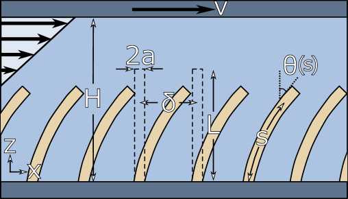
Figure 1: Illustration of how the fluid-hair system is modeled. Dashed and solid profiles show hairs in an undeformed and a deformed configuration, respectively. The model assumes the fluid velocity becomes zero at the hair-tip, exerting a shear stress $\frac{\eta v}{H-h(L)}$ on the hair.

Table 1: Important system parameters and their associated units

$H$	Channel height $[L]$
$L$	Hair length $[L]$
$a$	Hair radius $[L]$
$\phi$	Packing fraction
$\delta$	Hair-hair centerline spacing $[L]$
$E$	Elastic modulus $[M][T]^{-2}[L]^{-1}$
$I$	2nd area moment of hair’s cross-section $[L]^{4}$
$\eta$	Dynamic viscosity $[M][L]^{-1}[T]^{-1}$
$v$	Imposed fluid velocity $[L][T]^{-1}$
$\theta$	Angle between the local tangent and the vertical
$s$	Arc length measured from the base of the hair $[L]$

In this formulation the hair is represented as a plane curve in Cartesian coordinates with $\mathbf{R}=x(s)\hat{x}+z(s)\hat{z}$, where $\hat{x}$ and $\hat{z}$ are unit vectors. The unit tangent is given by $\hat{\mathbf{T}}=\sin\theta(s)\,\hat{x}+\cos\theta(s)\,\hat{z}$, so that $\hat{\mathbf{T}}\cdot\hat{z}=\cos\theta$, and with this parameterization the curvature is given by $d\theta/ds$. The quantity $h(s)=\int_{0}^{s}\cos\theta(s^{\prime})\,ds^{\prime}$ represents the height of the hair at position $s$ with $h(L)$ being the total height. Because the flow is horizontal (in the $\hat{x}$-direction), the force on the hair depends on its vertical height, and this is the reason for the denominator ${H-\int_{0}^{L}\cos\theta(s^{\prime})\,ds^{\prime}}=H-h(L)$ of (1): a vertical hair would be impacted by a maximum force, while the force is diminished as it entrains in the horizontal direction. A most interesting feature of this formulation is that the relaxed state that results is self-referential because of this denominator; i.e., the solution depends on itself and, as we will see, this gives rise to a self-consistency condition.

The form of (1) is obtained from moment balance in equilibrium. For an infinitesimal cylindrical section of a rod (the hair) this balance yields

$$\mathbf{M}(s+ds)-\mathbf{M}(s)+\mathrm{d}\mathbf{r}\times\mathbf{F}_{int}(s)=0\,,$$ (2)

where $\mathbf{M}(s)=EI\theta^{\prime}(s)\hat{\mathbf{y}}$ is the bending moment, $\mathrm{d}\mathbf{r}=\mathrm{d}s\hat{\mathbf{T}}(s)$, and $\mathbf{F_{int}}(s)$ is the net internal force on the rod segment. By “dividing” by $\mathrm{d}s$, we obtain (1). We refer the reader to Audoly and Pomeau (2010); Alvarado et al. (2017) for further details.

Equation (1) can be transformed into the compact nondimensional form

$$\frac{d^{2}\hat{\theta}}{d\sigma^{2}}=-\omega_{\epsilon}^{2}\cos\hat{\theta},$$ (3)

by introducing

$$\hat{\theta}(\sigma)=\theta(s)\,,\quad\sigma=\frac{s}{L}\,,\quad\epsilon=\frac{L}{H}\,,\quad\mathrm{and}\quad\omega^{2}=\frac{\pi a^{2}L^{2}\eta v}{EIH\phi}\,,$$ (4)

and

$$\omega_{\epsilon}^{2}=\frac{\omega^{2}}{1-\epsilon\int_{0}^{1}\cos\hat{\theta}(\sigma)\,d\sigma}\,.$$ (5)

The natural boundary conditions for (3) are the following:

$$\hat{\theta}(0)=\hat{\theta}_{0}\quad\mathrm{and}\quad\left.\frac{d\hat{\theta}}{d\sigma}\,\right|_{\sigma=1}\!\!\!\!=\,\hat{\theta}^{\prime}_{1}=0\,,$$ (6)

where $\hat{\theta}_{0}$ is the angle of attachment of the hair and ${\hat{\theta}}_{1}^{\prime}=0$ means that the hair at its tip has zero curvature. The latter condition can be obtained from the moment balance in Eq. 2. At the end of the hair, there is no upstream ($s>L$) contribution to the balance implying that $\hat{\mathbf{M}}(1)\equiv EI\hat{\theta}_{1}^{\prime}\hat{\mathbf{y}}$ is infinitesimally small. With these definitions, we see that our system has only two dimensionless parameters, $\epsilon$ and $\omega$, in addition to the choice of $\hat{\theta}_{0}$. We will drop the ‘hats’ moving forward to avoid clutter.

This system differs in some ways from the standard pendulum problem of mechanics. For example, we have the trivial difference that there is a shift in the definition of the angle – instead of having $\sin\theta$ on the righthand side of (3) we have $\cos\theta$. However, there are two essential differences: first, instead of the usual initial value problem, in light of (6), we have a boundary value problem and second, the system has the self-referential feature mentioned above, i.e., in order to know the effective frequency $\omega_{\epsilon}$ of (5) one must first obtain the entire “orbit” $\theta(\sigma)$ to get a self-consistent solution. Although these differences significantly complicate the problem, we will see that the problem remains integrable. We will see that the self-consistency condition together with the boundary value nature of the problem lead to a sort of quantization and a further reduction of parameters.

A “potential” for (3) can be obtained by setting $d^{2}\theta/d\sigma^{2}=-dV/d\theta$, where $V(\theta)=\omega^{2}_{\epsilon}\sin\theta$. The Hamiltonian of this system, which we will call $\mathcal{E}$, takes the form

$$\mathcal{E}=\frac{1}{2}\left(\frac{d\theta}{d\sigma}\right)^{2}+\omega^{2}_{\epsilon}\sin\theta\,.$$ (7)

Because $\omega_{\epsilon}$ does not depend explicitly on $\sigma$, the time-like variable, conservation of energy, $d\mathcal{E}/d\sigma=0$, follows immediately. Observe that the curvature, $d\theta/d\sigma$, determines a quantity analogous to the pendulum kinetic energy for this system.

As noted above, in the pendulum problem the potential is $-\cos\theta$ and the pendulum oscillates about $\theta=0$. However, the boundary value problem for the hair is different because the pendulum potential $-\cos\theta$ is shifted by $\pi/2$ from the hair’s potential, $\sin\theta$. Thus, the hair problem is analogous to a pendulum starting at $\theta=\theta_{0}$, a distance up the potential well, that is then projected further up the well with an initial velocity that is enough for it to hit its turning point at $d\theta/d\sigma=0$. Therefore, the goal is to determine the initial value of $d\theta/d\sigma$ corresponding to a time (length) for this to occur. To transform our problem to the pendulum problem we will shift $\theta$ by $\pi/2$, i.e.,

$$\bar{\theta}=\theta+\frac{\pi}{2}\qquad\Rightarrow\qquad\sin(\theta)=-\cos(\bar{\theta})\,,$$ (8)

and therefore

$$\mathcal{E}=\frac{1}{2}\left(\frac{d\bar{\theta}}{d\sigma}\right)^{2}\!-\,\omega^{2}_{\epsilon}\sin\bar{\theta}\,.$$ (9)

This angle shift is convenient because it allows us to write the solution in the standard form for the pendulum in terms of elliptic integrals, which is a first step toward showing integrability.

III Solution-Integrability

Given the formulation of Section II, we may begin by following the elementary procedure for reducing the pendulum to quadrature. Using the double-angle formula, $\cos\theta=1-2\sin^{2}(\theta/2)$, solving (9) for $d\bar{\theta}/d\sigma$, and integrating gives

$${\pm}\frac{\omega_{\epsilon}}{k}\,\sigma=\int^{\theta(\sigma)/2+\pi/4}_{{\theta_{0}}/{2}+\pi/4}\frac{d{\chi}}{\sqrt{1-k^{2}\sin^{2}\chi}}\,,$$ (10)

where $\chi=\theta/2$ and

$$k^{2}=\frac{2\omega_{\epsilon}^{2}}{\mathcal{E}+\omega_{\epsilon}^{2}}\,.$$ (11)

The choice in sign in (10) determines whether $\theta_{0}^{\prime}$ is positive or negative. While we are primarily interested in hairs with positive base-curvature (corresponding to the positive sign), we include both possibilities for completeness. This quadrature, analogous to that of the pendulum, is the first step toward obtaining integrability of our hair problem.

Before proceeding, there is one issue that must be checked, viz.  that $\sqrt{1-k^{2}\sin^{2}\chi}$ does not become imaginary; that is, we want to check that $k^{2}\sin^{2}\chi<1$ for $\chi$ within the limits of integration, and that this is maintained as the upper limit of the integral of (10) extends all the way to $\theta(1)$, which we will denote by $\theta_{1}$. For the most part, we expect physical solutions to have

$$0\leq\theta_{1}\leq\pi/2\,,$$ (12)

which we can verify after the solution is obtained, so that according to (7), $\mathcal{E}>0$. Thus, upon writing $\xi=\mathcal{E}/\omega^{2}_{\epsilon}$, (11) becomes $k^{2}=2/(1+\xi)$ with $\xi\geq 0$. Consequently,

$$1\leq k^{2}\leq 2\,,$$ (13)

and this by itself is insufficient to guarantee $k^{2}\sin^{2}\chi<1$, However, because of the second boundary condition of (6) and conservation of the energy of (9)

$$\xi=\sin\theta_{1}\quad\Rightarrow\quad 0\leq\xi\leq 1\,.$$ (14)

Next, using (12) and the fact that $\sin^{2}\chi$ achieves its maximum when $\theta=\theta_{1}$, we obtain

$$\sin^{2}\big{(}\theta_{1}/2+\pi/4\big{)}=\big{(}1+\sin\theta_{1}\big{)}/2\,,$$ (15)

which follows from elementary trigonometry identities. Therefore with (14), we have

$$k^{2}\sin\chi\leq\frac{2}{1+\xi}\,\frac{1}{2}\,\big{(}1+\sin\theta_{1}\big{)}=\frac{1}{1+\xi}\,\big{(}1+\xi\big{)}=1\,.$$ (16)

Thus the quadrature integral of (10) is well behaved even with $k^{2}>1$, which is consistent with what we would physically expect.

Proceeding, we can invert and obtain the explicit solution by writing the integral of (10) in terms of elliptic integrals. First, we split the integral as follows:

$${\pm}\frac{\omega_{\epsilon}}{k}\,\sigma=\hphantom{+}\int^{\theta(\sigma)/2+\pi/4}_{0}\frac{d\chi}{\sqrt{1-k^{2}\sin^{2}\chi}}-\int_{0}^{\theta_{0}/2+\pi/4}\frac{d\chi}{\sqrt{1-k^{2}\sin^{2}\chi}}\,,$$ (17)

and notice that the second integral of (17) is an incomplete elliptic integral of the first kind, which we move to the lefthand side, yielding

$${\pm}\frac{\omega_{\epsilon}}{k}\,\sigma+F\left(\left.\frac{\theta_{0}}{2}+\frac{\pi}{4}\,\right|k^{2}\right)=F\left(\left.\frac{\theta(\sigma)}{2}+\frac{\pi}{4}\,\right|k^{2}\right)\,.$$ (18)

Equation (18) can be inverted by utilizing Jacobi elliptic functions. In particular, the Jacobi amplitude function (see e.g. Abramowitz and Stegun (1965)) is the inverse of $F$ , i.e.,

$$\mathrm{am}\big{(}F(\phi|k^{2})|k^{2}\big{)}=\phi\,.$$ (19)

From now on we will drop the $k^{2}$ from the arguments and write $\mathrm{am}(\phi)$ for $\mathrm{am}(\phi\,|\,k^{2})$ and $F(\phi)$ for $F(\phi|k^{2})$, unless a different parameter is used. Using (19), (18) can be inverted to obtain the following solution:

$$\theta(\sigma)=2\,\mathrm{am}\left({\pm}\frac{\omega_{\epsilon}}{k}\,\sigma+F\left(\frac{\pi}{4}+\frac{\theta_{0}}{2}\right)\right)-\frac{\pi}{2}.$$ (20)

Evaluation of the Hamiltonian of (9) at $\sigma=0$ gives

$$\mathcal{E}=\frac{1}{2}\left({\theta_{0}^{\prime}}\right)^{2}+\omega_{\epsilon}^{2}\,\sin\theta_{0}\,,$$ (21)

where $\theta_{0}^{\prime}=d\theta(0)/d\sigma$. Using (11) and (21) we see that (20) gives $\theta(\sigma,\theta_{0},\theta_{0}^{\prime},\omega_{\epsilon})$, as expected for the solution of the initial value problem. To solve the boundary value problem where $\theta_{1}^{\prime}=0$ we use the identity ${d\,\mathrm{am}(u)}/{du}=\mathrm{dn}(u)$ and hence,

$$\frac{d\theta(\sigma)}{d\sigma}={\pm}2\,\frac{\omega_{\epsilon}}{k}\,\mathrm{dn}\left({\pm}\frac{\omega_{\epsilon}}{k}\,\sigma+F\left(\frac{\pi}{4}+\frac{\theta_{0}}{2}\right)\right),$$ (22)

and therefore the boundary condition gives

$$\theta_{1}^{\prime}={\pm}2\,\frac{\omega_{\epsilon}}{k}\,\mathrm{dn}\left({\pm}\frac{\omega_{\epsilon}}{k}+F\left(\frac{\pi}{4}+\frac{\theta_{0}}{2}\right)\right)=0\,.$$ (23)

Because elliptic integrals and functions usually consider the range $0\leq k^{2}\leq 1$, while we have (13), we use the identity

$$\mathrm{dn}(u\,|\,k^{2})=\mathrm{cn}(ku\,|\,k^{-2})$$ (24)

to write the boundary condition of (23) in the form

$$\mathrm{cn}\left({{\pm}\omega_{\epsilon}}+kF\left(\left.\frac{\pi}{4}+\frac{\theta_{0}}{2}\,\right|\,k^{2}\right)\Bigg{|}k^{-2}\right)=0\,.$$ (25)

Equation (25) gives a condition relating $\theta^{\prime}_{0}$ to ${\omega_{\epsilon}}$ for fixed $\theta_{0}$. Because of the periodic nature of cn$(u)$, these are quantized according to

$${\pm}{\omega_{\epsilon}}+kF\left(\left.{\pi}/{4}+{\theta_{0}}/{2}\,\right|\,k^{2}\right)={(2n+1)}K(k^{-2})\,,\qquad n\in\mathbb{Z}\,,$$ (26)

where $K(k^{-2})=F(\pi/2\,|\,k^{-2})$.

To summarize we collect all our parameters together,

$$k^{2}=\frac{2}{1+\xi}\,,\qquad\xi=\frac{\mathcal{E}}{\omega^{2}_{\epsilon}}\,,\qquad\mathcal{E}=\frac{1}{2}(\theta^{\prime}_{0})^{2}+{\omega_{\epsilon}}^{2}\sin\theta_{0}\,,$$

and observe, we have shown for fixed and given ${\omega_{\epsilon}}$ and $\theta_{0}$ the above analysis tells us what $\theta^{\prime}_{0}$ must be to hit our boundary condition $\theta_{1}^{\prime}=0$.

So far we have followed a conventional and straightforward path leading to the solution of (20). Except for the shift in phase and the boundary value nature of this solution, it is standard for a one degree-of-freedom Hamiltonian system: it depends on two parameters related to possible initial conditions $\theta_{0}$ and $\theta_{0}^{\prime}$ via $\mathcal{E}$ and one parameter $\omega_{\epsilon}$, which we have treated as a given constant. We proceed now by examining in general terms the boundary value nature of our problem with the imposition of the self-consistency constraint of (5).

Consider a general system of differential equations of the form

$$\frac{d^{2}\theta}{d\sigma^{2}}=f(\theta,\lambda)\,,$$ (27)

where $\lambda$ is a parameter. Often one uses a shooting method to solve the boundary value problems for equations of this type, i.e., a sequence of initial conditions are integrated numerically for choices of the parameter $\lambda$ until the desired boundary condition is reached. This procedure usually selects out discrete values for $\lambda$, which for linear systems would be eigenvalues. However, if one has an analytical solution to the initial value problem, as we do, this can be used to relate initial and final values. A condition that relates derivatives at the endpoints, here taken to be $\sigma=0$ and $\sigma=1$, follows immediately upon integrating (27), i.e.

$$\theta_{1}^{\prime}-\theta_{0}^{\prime}=\int_{0}^{1}f(\theta,\lambda)\,d\sigma\,.$$ (28)

Self-consistency means that the parameter $\lambda$ depends functionally on the solution $\theta(\sigma)$. For our problem at hand, the role played by $\lambda$ is $\omega_{\epsilon}$ and this self-consistency requires the solution of (20) be consistent with the $\omega_{\epsilon}$ as calculated from (5) with the insertion of (20). As a first step toward imposing this self-consistency constraint, analogous to (28) we integrate (3) to obtain an expression for the height of the hair in terms of an initial condition, viz.,

$$\theta_{0}^{\prime}=\omega_{\epsilon}^{2}\int_{0}^{1}\cos\theta(\sigma)\,d\sigma=\omega^{2}\frac{h_{1}}{1-\epsilon h_{1}}=\frac{1}{\epsilon}\,(\omega_{\epsilon}^{2}-\omega^{2})\,,$$ (29)

where $\theta_{0}^{\prime}=d\theta(0)/d\sigma$ and $h_{1}$ is the dimensionless height of the hair, the dimensional height being $h_{1}L$. The last equality of (29) follows upon eliminating $h_{1}$ using (5). The hair problem is complicated because the quantity $\omega^{2}_{\epsilon}$ depends on the solution of the boundary value problem (5) to give (29). Fortuitously, this quantity only depends on $h_{1}$, i.e., $\theta_{0}^{\prime}$ is proportional to $h_{1}$ and the constant of proportionality $\omega^{2}_{\epsilon}=\omega^{2}/({1-\epsilon h_{1}})$ also depends on $h_{1}$. For general problems of this nature of the form of (28), these two quantities would not in general depend on a single parameter like this.

Evidently, we must calculate $h_{1}$. In fact, we can explicitly calculate $h(\sigma)$ the height of the hair at parameter value $\sigma$ (see Appendix A),

$$h(\sigma) = \int_{0}^{\sigma}\!\cos\theta(\sigma^{\prime})\,d\sigma^{\prime}$$ (30)

$$= \frac{2}{k\omega_{\epsilon}}\left[\sqrt{1-k^{2}\sin^{2}({{\pi}/{4}+{\theta_{0}}/{2}})}-\mathrm{dn}\left({\pm}\frac{\omega_{\epsilon}}{k}\,\sigma+F\left({\pi}/{4}+{\theta_{0}}/{2}\right)\right)\right].$$

Next, we write $\omega_{\epsilon}$ in terms of $\omega$ and $\epsilon$ by inserting the last equality of (29) into (21), giving

$$\omega_{\epsilon}^{2}\,{\mp}\,\epsilon\sqrt{2\mathcal{E}-2\omega_{\epsilon}^{2}\sin\theta_{0}}=\omega^{2}\,.$$ (31)

Thus the self-consistent solution of our boundary value problem is fully determined by following:

$$\theta(\sigma;\theta_{0},\epsilon,\omega)=2\,\mathrm{am}\left({\pm}\omega_{\epsilon}\sqrt{\frac{\xi+1}{2}}\sigma+F\left(\frac{\pi}{4}+\frac{\theta_{0}}{2}\Big{|}\,k^{2}\right)\bigg{|}\,k^{2}\right)-\frac{\pi}{2}\,,$$ (32)

where $0\leq\sigma\leq 1$ is our dimensionless parameter and

$$0 = {\pm}{{\omega_{\epsilon}}+kF\left(\left.{\pi}/{4}+{\theta_{0}}/{2}\,\right|\,k^{2}\right)-(2n+1)K(k^{-2})}\,,$$ (33)

$$\omega_{\epsilon}^{2} = \omega^{2}\,{\pm}\,\epsilon\omega_{\epsilon}\sqrt{2\xi-2\sin\theta_{0}}\,,$$ (34)

$$k^{2} = \frac{2}{\xi+1}\,.$$ (35)

Note, $kF(\varphi|k^{2})=F(\bar{\varphi}|k^{-2})$, where $\sin\bar{\varphi}=k\sin\varphi$, (see equation (8.127) of Gradshteyn and Ryzhik (2007)) can be used when evaluating (33). Here (33) with (35) determines $\omega_{\epsilon}$ as a function of $\theta_{0}$ and $\xi$, which with (34) determines $\xi$ as a function of $\theta_{0}$, $\epsilon$, and $\omega$. We note in passing that the variable $\xi$ is related to the physically perspicuous variable $h_{1}$ according to

$$\xi=\frac{\omega^{2}}{2}\frac{h_{1}}{\left(1-\epsilon h_{1}\right)^{2}}+\sin\theta_{0}\,.$$

In Section IV we will evaluate (32) for various cases. We will see that for physically realizable solutions of interest, we must set $n=0$ in (33) and select the $+$ branch. In practice we use root finding to solve (33) and (34).

IV Phase Space Interpretation

Because (3) is isomorphic to the differential equation for a pendulum, it is helpful to interpret our analytical solutions in terms of motion in the pendulum phase space. In this section we do this, first for hairs with $\theta_{0}=0$ and then for $\theta_{0}\neq 0$.

IV.1 Vertical hairs: $\theta_{0}=0$

Figure 2 shows several different trajectories, corresponding to different values of $\xi$, for the case where $\theta_{0}=0$. Here, only the solutions that stop when they intersect $\theta_{1}^{\prime}=0$ once are shown, but we do observe other solutions corresponding to trajectories completing one or several orbits, especially at higher values of $\xi$.

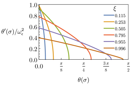
Figure 2: Phase portraits for a selected set of $0\leq\xi\leq 1$, a scaled measure of the energy, and their corresponding profiles. $\xi=1$ corresponds with the separatrix. Trajectories start at $\theta(0)=0$ and end at $\theta^{\prime}(1)=0$.

Observe, $\xi={\mathcal{E}}/{\omega_{\epsilon}^{2}}$ and $\mathcal{E}$ are both measures of the system’s energy (Hamiltonian) since they only differ by a proportionality constant, once self-consistency is enforced. We prefer to use $\xi$ in the following figures and analysis because $-1\leq\xi\leq 1$, while $\mathcal{E}$ is unbounded. In addition, our analytic solution is written more concisely in terms of $\xi$. Figure 2 shows the phase space with energy surfaces parameterized by $\xi$. Note, because $\xi$ is used and because the ordinate is $\theta^{\prime}/\omega_{\epsilon}^{2}$, the energy surfaces are not nested as usual. In Fig. 2, as $\xi\rightarrow 1$ the orbit approaches the separatrix (within the pendulum analogy, a value of $\xi=1$ corresponds to a pendulum “kicked” up from $\theta_{0}=0$ to $\theta_{1}=\frac{\pi}{2}$) and $\xi=0$ corresponds to the undeformed hair where $\theta(\sigma)\equiv 0$.

Within the pendulum analogy, a fixed choice of $\omega_{\epsilon}$ is related to a choice of gravitational acceleration. The boundary conditions $\theta_{0}=0$ and $\theta^{\prime}_{1}=0$ describe a pendulum trajectory starting at $\theta=0$ and ending when $\dot{\theta}=0$ in a time $T$ (analogous to the length of a hair). The largest possible initial velocity (or energy) that satisfies these conditions corresponds to a phase-space trajectory entirely confined to the first quadrant. At a threshold, other starting velocities can also satisfy the “initial” conditions, but they must correspond to orbits that exit the first quadrant.

Figure 3 depicts two orbits for a given choice of parameters. The first (black) starts at $\theta_{0}=0$ with some $\dot{\theta}_{0}\neq 0$ and the trajectory evolves until $\dot{\theta}_{1}=0$. On the other hand, the blue orbit reaches its first maximum when $\dot{\theta}(t=1/3)=0$ and it oscillates the other direction until finally reaching $\dot{\theta}_{1}=0$. When not equal to zero, the branch index, $n$ (shown in Eq. 32) selects out these lower period orbits. In addition to these two solutions in our example above, there are two more with an opposite sign in $\dot{\theta}_{0}$. This choice in direction is reflected by the $\pm$ sign in our solution.

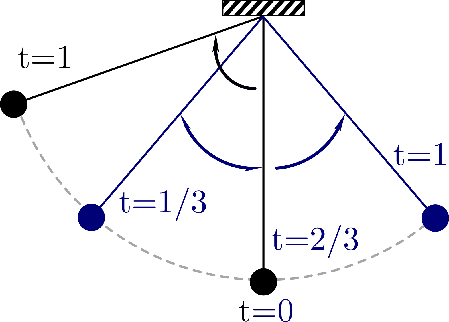
Figure 3: The problem of a cantilevered hair with a point load at its end is isomorphic to the equation of motion for a pendulum with the initial conditions $\theta(t=0)=0$ and $\dot{\theta}(t=1)$=0. Because multiple different orbits can satisfy these conditions for a given choice in parameters (e.g., the blue and black orbits of the figure), both the cantilevered hair and pendulum problem posed above are not unique.

For the hairs, choices of $n\neq 0$ and/or negative curvature branches correspond to “twirling” profiles (see Fig. 4). These orbits are not physically realizable for simple shear flow experiments for either of two reasons:

• Hair profiles intersect the surface they are mounted on (or also themselves). This is possible because the model does not consider hair-surface interactions.

• The assumption that shear stress is concentrated at the hair tip breaks down because the hair-tip is no longer the portion exposed to shear flow.

These solutions are an important consideration nevertheless because numerical algorithms can be susceptible to converging to them.

All accessible solutions for a discrete list of $\epsilon$ values and a range of $\omega^{2}$ are plotted in Fig. 4. In panel (a) we plot the energy $\mathcal{E}$ (a measure of $\theta_{0}^{\prime}$) vs. $\omega^{2}$ for the values of $\epsilon$ color coded in panel (c). The blue curve corresponds to $\epsilon=0$, the case where self-consistency vanishes, while the orange curve shows the distortion caused as $\epsilon$ approaches unity. This plot makes it clear that the pendulum analogy alone is insufficient to capture predictions of the basic model. Panel (b) shows that the solutions of the self-consistent boundary value problem are completely collapsed when the similarity variable $\xi$ is used instead of $\mathcal{E}$. In this plot of $\xi$ vs. $\omega_{\epsilon}^{2}$ there is only a single curve. The black lines on this plot depict representative hair profiles: for small $\omega_{\epsilon}^{2}$ the hair only slightly bends while there is a scaling change for $\omega_{\epsilon}^{2}\gtrsim 1$ as the hair bends significantly. In addition, for larger $\omega_{\epsilon}^{2}$ we obtain the twirling profiles where the solid and dashed lines of panel (b) indicate positive and negative base curvature, respectively. Panel (c) shows that the physically realizable branch can be partially collapsed by plotting $\xi$ vs.  $\omega^{2}/(1-\epsilon)$. In the case of the physically realizable solutions, the dependence on $\epsilon$ is most apparent for small forcing where the hair height is maximal. For this case (e.g. small imposed fluid velocity $v<<1$) $h_{1}\rightarrow 1$, i.e., the hair is nearly vertical with $\theta\approx 0$. Thus from (29), $\theta_{0}^{\prime}\approx\omega_{\epsilon}^{2}$, which with (21) gives

$$\xi=\frac{\theta^{\prime 2}}{2\omega_{\epsilon}^{2}}+\sin{\theta}\approx\frac{\theta^{\prime 2}}{2\omega_{\epsilon}^{2}}\approx\frac{\omega_{\epsilon}^{2}}{2}\,.$$ (36)

This explains the linear dependence and slope observed in panel (b) of Fig. 4 for small $\omega_{\epsilon}^{2}$. For large forcing where $\omega^{2}\rightarrow\infty$, the height of the hair asymptotically approaches zero, i.e., $\theta_{1}\approx\pi/2$ and $\xi\approx\sin{\theta_{1}}\approx 1$, which explains the asymptote of panel (b) of Fig. 4. In this limit $\omega_{\epsilon}^{2}\rightarrow\omega^{2}$ and the $\epsilon$-dependence vanishes. Finally, one expects the crossover between weak and strong forcing behavior to occur near ${\omega_{\epsilon}^{2}}/{2}\approx 1$, and indeed this is the case.

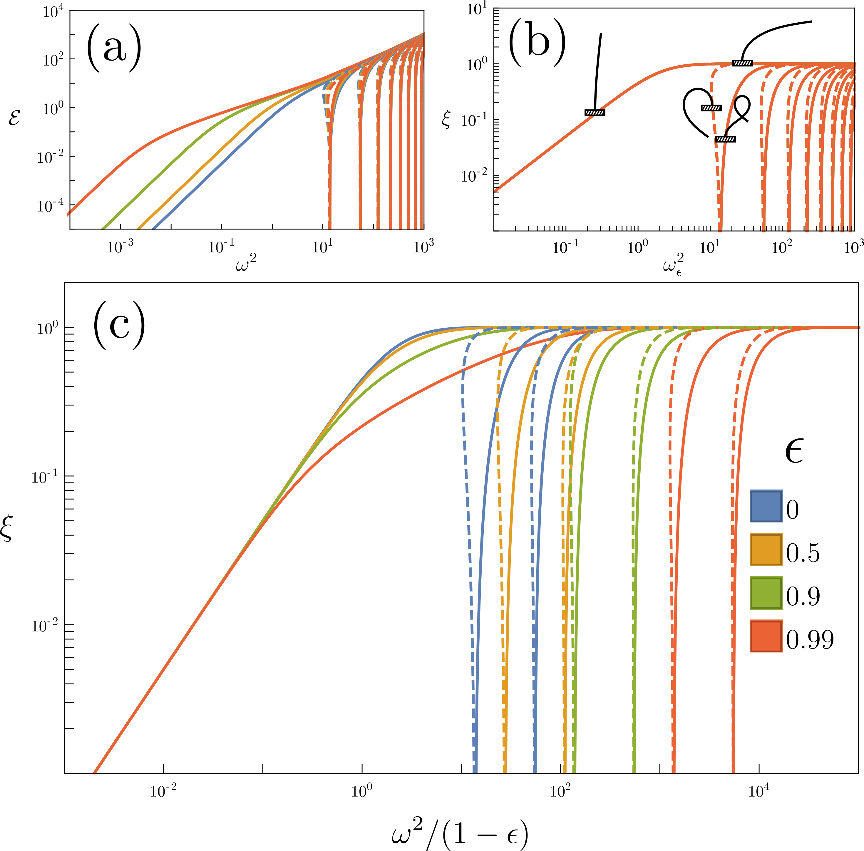
Figure 4: Plots of solutions of the boundary value problem posed in Section II for the case $\theta_{0}=0$ depending on the two parameters, $\omega^{2}$ and $\epsilon$. (a) Uncollapsed dependence of the energy (Hamiltonian) $\mathcal{E}$ on the two input parameters. (b) Fully collapsed solution space in terms of the similarity variables $\xi=\mathcal{E}/\omega_{\epsilon}^{2}$ vs. $\omega_{\epsilon}^{2}$, with representative hair profiles. Here, solid and dashed lines indicate positive and negative base curvature, respectively. Note, $\omega_{\epsilon}^{2}$ is a quantity that depends transcendentally on $\omega^{2}$ and $\epsilon$. For weak and strong forcing we see the predicted scalings of $\xi\approx\omega_{\epsilon}^{2}/2$ and $\xi\rightarrow 1$, respectively, with the crossover occurring near ${\omega_{\epsilon}^{2}}/{2}\approx 1$. (c) Partial collapse of the solution space is seen using the abscissa $\omega^{2}/(1-\epsilon)$, showing physically realizable branches with an explicit function of the input parameters. To avoid clutter, only the first three branches (and their negative curvature counterparts) are plotted in this panel.

IV.2 Angled hairs: $\theta_{0}\neq 0$

Next, we plot $\xi$ vs.  $\omega_{\epsilon}$ for different values of $\theta_{0}$ in Fig. 5. For negative $\theta_{0}$, shear flow is against the grain. As the forcing increases, hairs reorient to align with the fluid velocity until $\theta_{1}=0$ which corresponds to $\xi=0$. Further increasing the forcing parameter brings the system into the flow alignment regime, scaling the same for all $\theta_{0}$.

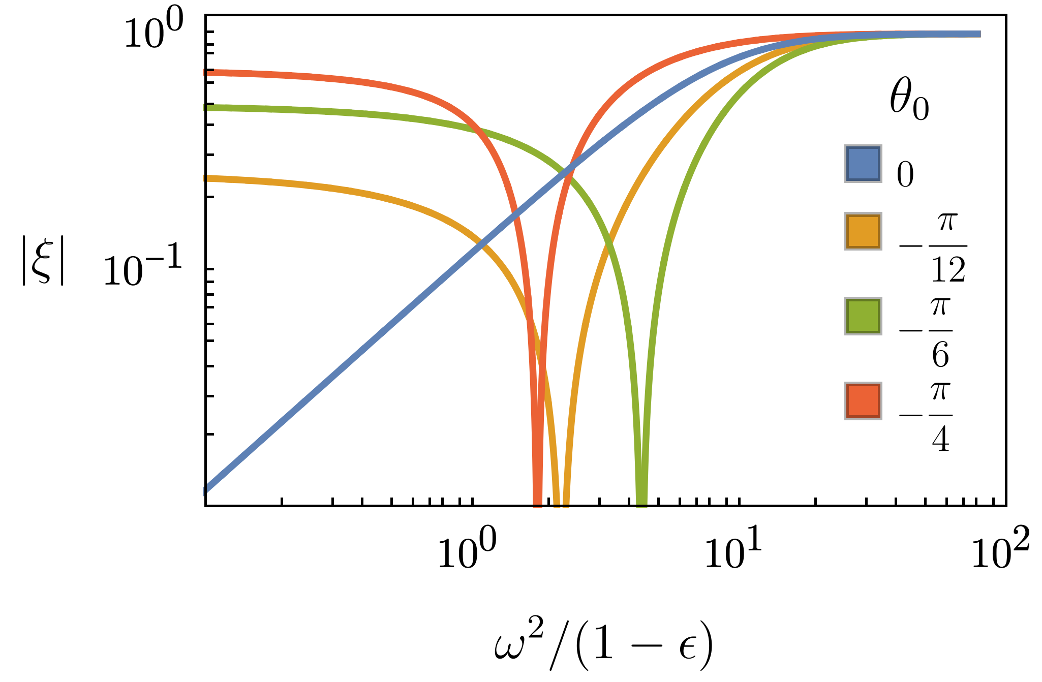
Figure 5: $\xi$ vs $\omega_{\epsilon}$ plotted using Eq. 32 for different values of $\theta_{0}$. Hairs with a negative base-angle have negative energy at low $\omega$, and transition to positive energy as $\omega$ increases. Figure created with $\epsilon=0.61$

On the other hand, increasing $\theta_{0}$ results in flow with the grain. Flow alignment can be achieved with a smaller forcing parameter (compared to $\theta_{0}=0$) and the dependence of $\xi$ on $\omega^{2}/(1-\epsilon)$ approaches a horizontal line.

V Hair profiles, discussion, and comparisons

Recall from Section II, the unit tangent is given by ${\mathbf{R}^{\prime}}=\hat{\mathbf{T}}$ which implies $x^{\prime}(\sigma)=\sin\theta(\sigma)$ and $z^{\prime}(\sigma)=\cos\theta(\sigma)$. Thus, given our solutions of Section III for $\theta(\sigma)$, we can plot $z$ vs. $x$ for the hair profiles. In this section we compare hair profiles obtained by our analytic solutions with those obtained by direct numerical integration. A standard numerical method for nonlinear boundary value problems is to use a shooting code, whereby initial values are incremented until the desired boundary value is obtained. In Alvarado et al. (2017) such a shooting code with a standard ordinary differential equation algorithm was used to integrate the pendulum equations of (1), with an adaptation allowing for the $\theta$-dependence in $\omega_{\epsilon}$. Another approach is to make a central difference approximation to the second derivative of (1), representing $\theta$ along the centerline of the hair by a mesh of $N$ segments with values $\theta_{i}$ ($i=1,2,...,N$). This gives a sequence of algebraic equations with the boundary conditions built into the first and last equation. Coupling of the equations is provided by both the differencing and the self-consistency through $\omega_{\epsilon}$. An example of this procedure is given in Gazzola et al. (2018), where the more complicated problem of a filament subject to three dimensional dynamical behavior is solved by discretizing in both space and time. Associated with this method is a root finding problem, which for the time-independent case involves solving $N$ equations for each mesh value $\theta_{i}$. Because there isn’t a concise description of how each of $\theta_{i}$ asymptotically scales with the forcing parameter, $\omega$, convergence to physical solutions is not always guaranteed.

In Fig. 6 a set of profiles is shown, comparing our analytic solution with numerical solutions obtained by using the mesh discretization described above. At low forcing, both approaches converge to the same, physical solution. At high forcing when the hair becomes more streamlined, the numerical solution requires a larger number of mesh segments in order to fully resolve the high curvature section at the base of the hair and so it does not fully agree with the analytic solution.

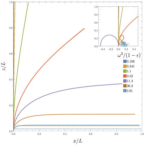
Figure 6: Comparison of numerical and analytic solutions for a variety of $\mathcal{E}$. Solid and dashed curves indicate numerical and analytic solutions, respectively. A discretization method was used for the numerical routine with an initial estimate of $\theta_{i}=0$ for the outer figure and $\theta_{i}=-0.1$ for the inset. For large $\omega$, the numerical solution requires many mesh segments in order to fully resolve the curvature at the base of the hair.

Even though there is a root finding problem associated with our analytic solution, it is a single equation (compared to $N$ for the numerical approach). Because of this, and the fact that we know how $\mathcal{E}$ scales in both deformed and undeformed regimes, our analytic method is both simpler to implement and faster to computed than numerical approaches.

We have observed that the analytic solution is about two orders of magnitude faster ($0.005$ s vs.  $0.5$ s for a finite-difference simulation with a mesh-size of 80) than the numerical procedure. There is not much difference in obtaining a single solution using either approach in terms of speed. However, problems that involve solving (3) iteratively can benefit significantly from the analytic approach. For example, optimization of the system’s rectification properties and solving weakly time-dependent problems ($\omega_{\epsilon}\rightarrow\omega_{\epsilon}(t)$) are potentially computationally expensive tasks.

Given a shear stress, what are the profiles of bed of hairs, which can be dense yet noninteracting? Our solution presented in (32) provides an answer to this question. The inverse problem, where the profiles are used to infer the shear stress, is utilized in a recently developed imaging technique. In Liu et al. (2019); Brücker (2015), a bed of flexible micropillars is used to detect near-wall shear stress and velocity fields in turbulent flow. The pillars act as wave guides allowing the tip deflection to be measured when illuminated from below. Our analytic method could be used to derive simple expressions for tip-deflection, which can be utilized in the linear, low deformation regime. Greater flow-detection sensitivity can be achieved by increasing the flexibility of the pillars and operating them in the nonlinear regime Brücker (2015).

Lastly, we argue that our analytic solution can be used as a basis for understanding problems where the fluid flow has a slow time dependence. In this regime, a hair cycles through its steady-state profiles, and fluid flows within the hair bed can be neglected.

VI Summary

In this work, we obtained a solution to a differential equation describing the profile of a hair bed immersed in shear flow. This problem differs from previous treatments of cantilevered rods in that the forcing parameter has functional dependence on the dependent variable, $\theta(\sigma)$. As a result, the spectrum of permissible $\omega_{\epsilon}$ at fixed $\xi$ becomes continuous in addition to being discrete. As interesting as they are, many of these solutions are not physically realizable and an advantage of our analytic work is that we can select the desired branch. To contrast this, shooting codes and other numerical approaches cannot be guaranteed to converge to this class of solution.

We then compare the analytic solution to a central difference based numerical scheme that performs reasonably well for the range of loading tested, but can encounter a convergence issue when the curvature at the base is large.

Future work could explore an adiabatic extension of this model to describe time-dependent channel flows.

Appendix A Calculation of $h(\sigma)$

We wish to calculate $h(\sigma)$ of (30). To this end, let

$$\theta(\sigma)=2\left[\mathrm{am}\left(u\right)-{\pi}/{4}\right]\quad\mathrm{with}\quad u:=\frac{\omega_{\epsilon}}{k}\,\sigma+F\left(\frac{\pi}{4}+\frac{\theta_{0}}{2}\right)\,.$$ (37)

Using elementary trigonometry identities we obtain

$$\cos\theta(\sigma)=\cos\Big{[}2\,\big{(}\mathrm{am}(u)-\pi/4\big{)}\Big{]}=1-2\sin^{2}[\mathrm{am}(u)-\pi/4]\,,$$ (38)

$$\sin\big{(}\mathrm{am}(u)-\pi/4\big{)}=\frac{\sqrt{2}}{2}\big{(}\mathrm{sn}(u)-\mathrm{cn}(u)\big{)}\,,$$ (39)

with the identities sn$(u)=\sin\big{(}\mathrm{am}(u)\big{)}$ and cn$(u)=\cos\big{(}\mathrm{am}(u)\big{)}$. Thus,

$$2\sin^{2}\big{(}\mathrm{am}(u)-\pi/4\big{)}=\big{(}\mathrm{sn}(u)-\mathrm{cn}(u)\big{)}^{2}=1-2\mathrm{cn}(u)\mathrm{sn}(u)\,,$$ (40)

using $\mathrm{sn}^{2}(u)+\mathrm{cn}^{2}(u)=1$. So $1-2\sin^{2}(u)=2\mathrm{cn}(u)\mathrm{sn}(u)$, which with

$$\mathrm{cn}(u)\mathrm{sn}(u)=-\frac{1}{k^{2}}\frac{d}{du}\mathrm{dn}(u)$$ (41)

we obtain

$$\int_{0}^{\sigma}\cos\theta(\sigma^{\prime})\,d\sigma^{\prime}=-\frac{k}{\omega_{\epsilon}}\,\frac{2}{k^{2}}\int_{u_{0}}^{u}\frac{d}{du^{\prime}}\mathrm{dn}(u^{\prime})\,du^{\prime}=\frac{2}{k\omega_{\epsilon}}\big{(}\mathrm{dn}(u_{0})-\mathrm{dn}(u)\big{)}$$ (42)

using $d\sigma={k}\,du/{\omega_{\epsilon}}$, where $u_{0}=F\left({\pi}/{4}+{\theta_{0}}/{2}\right)$. Finally we use

$$\mathrm{dn}\big{(}F(\phi|k^{2})\big{)}=\sqrt{1-k^{2}\sin^{2}\phi}$$ (43)

to obtain the result of (30).

References

- Autumn et al. (2002) K. Autumn, M. Sitti, Y. A. Liang, A. M. Peattie, W. R. Hansen, S. Sponberg, T. W. Kenny, R. Fearing, J. N. Israelachvili, and R. J. Full, Proceedings of the National Academy of Sciences 99, 12252 (2002), ISSN 0027-8424, 1091-6490, publisher: National Academy of Sciences Section: Biological Sciences, URL https://www.pnas.org/content/99/19/12252.
- Cummins et al. (2007) B. Cummins, T. Gedeon, I. Klapper, and R. Cortez, Journal of theoretical biology 247, 266 (2007), ISSN 0022-5193, URL https://www.ncbi.nlm.nih.gov/pmc/articles/PMC2742163/.
- Harper et al. (2013) C. J. Harper, S. M. Swartz, and E. L. Brainerd, Proceedings of the National Academy of Sciences 110, 8852 (2013), ISSN 0027-8424, 1091-6490, publisher: National Academy of Sciences Section: Biological Sciences, URL https://www.pnas.org/content/110/22/8852.
- Reicher and Uni (2021) N. Reicher and Z. Uni, Poultry Science 100, 101401 (2021), ISSN 0032-5791, URL https://www.sciencedirect.com/science/article/pii/S0032579121004247.
- Zou et al. (2019) Y.-N. Zou, D.-J. Zhang, C.-Y. Liu, and Q.-S. Wu, Pakistan Journal of Botany 51 (2019), ISSN 05563321, 20703368, URL http://pakbs.org/pjbot/paper_details.php?id=8535.
- Luhar and Nepf (2011) M. Luhar and H. M. Nepf, Limnology and Oceanography 56, 2003 (2011), ISSN 1939-5590, _eprint: https://onlinelibrary.wiley.com/doi/pdf/10.4319/lo.2011.56.6.2003, URL https://onlinelibrary.wiley.com/doi/abs/10.4319/lo.2011.56.6.2003.
- Weinbaum et al. (2021) S. Weinbaum, L. M. Cancel, B. M. Fu, and J. M. Tarbell, Cardiovascular Engineering and Technology 12, 37 (2021), ISSN 1869-4098, URL https://doi.org/10.1007/s13239-020-00485-9.
- Chateau et al. (2019) S. Chateau, J. Favier, S. Poncet, and U. D’Ortona, Physical Review E 100, 042405 (2019), publisher: American Physical Society, URL https://link.aps.org/doi/10.1103/PhysRevE.100.042405.
- Angleys and Østergaard (2020) H. Angleys and L. Østergaard, American Journal of Physiology-Heart and Circulatory Physiology 318, H425 (2020), ISSN 0363-6135, 1522-1539, URL https://www.physiology.org/doi/10.1152/ajpheart.00384.2019.
- Walker et al. (1985) G. Walker, A. B. Yulf, and J. Ratcliffe, Journal of Zoology 205, 297 (1985), ISSN 1469-7998, _eprint: https://onlinelibrary.wiley.com/doi/pdf/10.1111/j.1469-7998.1985.tb03536.x, URL https://onlinelibrary.wiley.com/doi/abs/10.1111/j.1469-7998.1985.tb03536.x.
- Bullock and Federle (2011) J. M. R. Bullock and W. Federle, Naturwissenschaften 98, 381 (2011), ISSN 0028-1042, 1432-1904, URL http://link.springer.com/10.1007/s00114-011-0781-4.
- Suter et al. (2004) R. B. Suter, G. E. Stratton, and P. R. Miller, The Journal of Arachnology 32, 11 (2004), ISSN 0161-8202, 1937-2396, publisher: American Arachnological Society, URL https://bioone.org/journals/the-journal-of-arachnology/volume-32/issue-1/M02-74/TAXONOMIC-VARIATION-AMONG-SPIDERS-IN-THE-ABILITY-TO-REPEL-WATER/10.1636/M02-74.full.
- Kim et al. (2011) W. Kim, T. Gilet, and J. W. M. Bush, Proceedings of the National Academy of Sciences of the United States of America 108, 16618 (2011), ISSN 0027-8424, URL https://www.ncbi.nlm.nih.gov/pmc/articles/PMC3189050/.
- Nasto et al. (2018) A. Nasto, P.-T. Brun, and A. E. Hosoi, Physical Review Fluids 3, 024002 (2018), publisher: American Physical Society, URL https://link.aps.org/doi/10.1103/PhysRevFluids.3.024002.
- Guo et al. (2000) P. Guo, A. M. Weinstein, and S. Weinbaum, American Journal of Physiology. Renal Physiology 279, F698 (2000), ISSN 1931-857X.
- Hood et al. (2019) K. Hood, M. S. S. Jammalamadaka, and A. E. Hosoi, Physical Review Fluids 4, 114102 (2019), ISSN 2469-990X, URL https://link.aps.org/doi/10.1103/PhysRevFluids.4.114102.
- Thomazo et al. (2019) J.-B. Thomazo, J. Contreras Pastenes, C. J. Pipe, B. Le Révérend, E. Wandersman, and A. M. Prevost, Journal of The Royal Society Interface 16, 20190362 (2019), ISSN 1742-5689, 1742-5662, URL https://royalsocietypublishing.org/doi/10.1098/rsif.2019.0362.
- Thomazo et al. (2020) J.-B. Thomazo, E. Lauga, B. Le Révérend, E. Wandersman, and A. M. Prevost, Physical Review E 102, 010602 (2020), ISSN 2470-0045, 2470-0053, URL https://link.aps.org/doi/10.1103/PhysRevE.102.010602.
- Takagi and Strickler (2020) D. Takagi and J. R. Strickler, Scientific Reports 10, 2665 (2020), ISSN 2045-2322, URL http://www.nature.com/articles/s41598-020-58880-0.
- Chagnaud et al. (2008) B. P. Chagnaud, C. Brücker, M. H. Hofmann, and H. Bleckmann, Journal of Neuroscience 28, 4479 (2008), ISSN 0270-6474, eprint https://www.jneurosci.org/content/28/17/4479.full.pdf, URL https://www.jneurosci.org/content/28/17/4479.
- Dangles et al. (2006) O. Dangles, D. Pierre, C. Magal, F. Vannier, and J. Casas, Journal of Experimental Biology 209, 4363 (2006), ISSN 0022-0949, eprint https://journals.biologists.com/jeb/article-pdf/209/21/4363/1541696/4363.pdf, URL https://doi.org/10.1242/jeb.02485.
- Sutton et al. (2016) G. P. Sutton, D. Clarke, E. L. Morley, and D. Robert, Proceedings of the National Academy of Sciences 113, 7261 (2016), ISSN 0027-8424, 1091-6490, publisher: National Academy of Sciences Section: Biological Sciences, URL https://www.pnas.org/content/113/26/7261.
- du Roure et al. (2019) O. du Roure, A. Lindner, E. N. Nazockdast, and M. J. Shelley, Annual Review of Fluid Mechanics 51, 539 (2019), ISSN 0066-4189, 1545-4479, URL https://www.annualreviews.org/doi/10.1146/annurev-fluid-122316-045153.
- Nasto et al. (2016) A. Nasto, M. Regli, P.-T. Brun, J. Alvarado, C. Clanet, and A. E. Hosoi, Physical Review Fluids 1, 033905 (2016), ISSN 2469-990X, URL https://link.aps.org/doi/10.1103/PhysRevFluids.1.033905.
- Hanasoge et al. (2017) S. Hanasoge, M. Ballard, P. J. Hesketh, and A. Alexeev, Lab on a Chip 17, 3138 (2017), ISSN 1473-0189, publisher: The Royal Society of Chemistry, URL https://pubs.rsc.org/en/content/articlelanding/2017/lc/c7lc00556c.
- Zhang et al. (2021a) X. Zhang, J. Guo, X. Fu, D. Zhang, and Y. Zhao, Advanced Intelligent Systems 3, 2000225 (2021a), ISSN 2640-4567, _eprint: https://onlinelibrary.wiley.com/doi/pdf/10.1002/aisy.202000225, URL https://onlinelibrary.wiley.com/doi/abs/10.1002/aisy.202000225.
- Wang et al. (2016) Y. Wang, J. d. Toonder, R. Cardinaels, and P. Anderson, Lab on a Chip 16, 2277 (2016), ISSN 1473-0189, publisher: The Royal Society of Chemistry, URL https://pubs.rsc.org/en/content/articlelanding/2016/lc/c6lc00531d.
- Paek and Kim (2014) J. Paek and J. Kim, Nature Communications 5, 3324 (2014), ISSN 2041-1723, bandiera_abtest: a Cg_type: Nature Research Journals Number: 1 Primary_atype: Research Publisher: Nature Publishing Group Subject_term: Design, synthesis and processing Subject_term_id: design-synthesis-and-processing, URL https://www.nature.com/articles/ncomms4324.
- Zhang et al. (2021b) S. Zhang, Z. Cui, Y. Wang, and J. den Toonder, ACS Applied Materials & Interfaces 13, 20845 (2021b), ISSN 1944-8244, publisher: American Chemical Society, URL https://doi.org/10.1021/acsami.1c03009.
- Milana et al. (2020) E. Milana, R. Zhang, M. R. Vetrano, S. Peerlinck, M. De Volder, P. R. Onck, D. Reynaerts, and B. Gorissen, Science Advances 6, eabd2508 (2020), publisher: American Association for the Advancement of Science, URL https://www.science.org/doi/10.1126/sciadv.abd2508.
- Alvarado et al. (2017) J. Alvarado, J. Comtet, E. de Langre, and A. E. Hosoi, Nature Physics 13, 1014 (2017), ISSN 1745-2481, bandiera_abtest: a Cg_type: Nature Research Journals Number: 10 Primary_atype: Research Publisher: Nature Publishing Group Subject_term: Biological physics;Fluid dynamics Subject_term_id: biological-physics;fluid-dynamics, URL https://www.nature.com/articles/nphys4225.
- Stein and Shelley (2019) D. B. Stein and M. J. Shelley, Physical Review Fluids 4, 073302 (2019), ISSN 2469-990X, URL https://link.aps.org/doi/10.1103/PhysRevFluids.4.073302.
- Shanko et al. (2019) E.-S. Shanko, Y. van de Burgt, P. D. Anderson, and J. M. J. den Toonder, Micromachines 10, 731 (2019), number: 11 Publisher: Multidisciplinary Digital Publishing Institute, URL https://www.mdpi.com/2072-666X/10/11/731.
- Zhang et al. (2021c) R. Zhang, J. den Toonder, and P. R. Onck, Physics of Fluids 33, 092009 (2021c), ISSN 1070-6631, publisher: American Institute of Physics, URL https://aip.scitation.org/doi/10.1063/5.0054929.
- Saberi et al. (2019) A. Saberi, S. Zhang, C. v. d. Bersselaar, H. Kandail, J. M. J. d. Toonder, and N. A. Kurniawan, Soft Matter 15, 1435 (2019), ISSN 1744-6848, publisher: The Royal Society of Chemistry, URL https://pubs.rsc.org/en/content/articlelanding/2019/sm/c8sm01957f.
- Audoly and Pomeau (2010) B. Audoly and Y. Pomeau, Elasticity and Geometry: From hair curls to the nonlinear response of shells (Oxford University Press, Oxford ; New York, 2010), illustrated edition ed., ISBN 978-0-19-850625-6.
- Luminari (2018) N. Luminari, Ph.D. thesis, Université de Toulouse (2018).
- Petrovic et al. (2006) L. Petrovic, M. Henne, and J. Anderson, Volumetric methods for simulation and rendering of hair (2006).
- Ryu (2007) D. Ryu, 500 million and counting: Hair rendering on ratatouille (2007).
- Iben et al. (2013) H. Iben, M. Meyer, L. Petrovic, O. Soares, J. Anderson, and A. Witkin, in Proceedings of the 12th ACM SIGGRAPH/Eurographics Symposium on Computer Animation - SCA ’13 (ACM Press, Anaheim, California, 2013), p. 63, ISBN 978-1-4503-2132-7, URL http://dl.acm.org/citation.cfm?doid=2485895.2485913.
- Abramowitz and Stegun (1965) M. Abramowitz and I. A. Stegun, eds., Handbook of Mathematical Functions: with Formulas, Graphs, and Mathematical Tables (Dover Publications, New York, NY, 1965), 0009th ed., ISBN 978-0-486-61272-0.
- Gradshteyn and Ryzhik (2007) I. S. Gradshteyn and I. M. Ryzhik, Table of integrals, series, and products (Elsevier/Academic Press, Amsterdam, 2007), seventh ed., ISBN 978-0-12-373637-6; 0-12-373637-4, translated from the Russian, Translation edited and with a preface by Alan Jeffrey and Daniel Zwillinger, With one CD-ROM (Windows, Macintosh and UNIX).
- Gazzola et al. (2018) M. Gazzola, L. H. Dudte, A. G. McCormick, and L. Mahadevan, Royal Society Open Science 5, 171628 (2018), ISSN 2054-5703, URL https://royalsocietypublishing.org/doi/10.1098/rsos.171628.
- Liu et al. (2019) Y. Liu, M. Klaas, and W. Schröder, Experimental Thermal and Fluid Science 106, 171 (2019), ISSN 0894-1777, URL https://www.sciencedirect.com/science/article/pii/S0894177718319708.
- Brücker (2015) C. Brücker, Physics of Fluids 27, 031705 (2015), ISSN 1070-6631, 1089-7666, URL http://aip.scitation.org/doi/10.1063/1.4916768.