Trie-based ranking of quantum many-body states

Abstract

Ranking bit patterns—finding the index of a given pattern in an ordered sequence—is a major bottleneck scaling up numerical quantum many-body calculations, as fermionic and hard-core bosonic states translate naturally to bit patterns. Traditionally, ranking is done by bisectioning search, which has poor cache performance on modern machines. We instead propose to use tries (prefix trees), thereby achieving a two- to ten-fold speed-up in numerical experiments with only moderate memory overhead. For the important problem of ranking permutations, the corresponding tries can be compressed. These compressed “staggered” lookups allow for a considerable speed-up while retaining the memory requirements of prior algorithms based on the combinatorial number system.

I Introduction

At their first encounter with the quantum many-fermion problem, students are usually warned that any brute-force attempt at a solution is destined to shatter at the exponential wall—the doubling of computing requirements with the addition of each state. Commonly, this then segues into the presentation of some polynomial-cost approximation.

So it is perhaps ironic that the brute-force solution of small many-fermion problems, known as exact diagonalization (ED) [Bonner64, Alvermann2011, Innerberger2020], many-body Lanczos method [Lanczos1950, Cullum1985], or full-configuration interaction (FullCI) [Siegbahn84, Knowles84], has remained one of the workhorses of many-body physics and quantum chemistry. On small systems, it serves as benchmark for more advanced (classical [Motta17] or quantum computing [Gheorghiu19R]) methods and to explore emergent many-body behavior [Sandvik10ACP]. For realistic systems, exact diagonalization is particularly useful as kernel of embedding theories [DMFT, DMET, SEET], where one approximately maps the full problem onto one or more difficult but small many-body problems. In that problem space, ED is competing with Monte Carlo methods [Gull2011, w2dynamics], which do not have as severe a restriction in system size, but usually require sufficient symmetry to avoid a prohibitive sign problem. An iterative ED is also at the core of more sophisticated renormalization schemes, most notably the numerical renormalization group (NRG) [Bulla2008] and density matrix renormalization group (DMRG) [Schollwock2005] method.

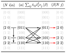
Figure 1: On-the-fly construction of the matrix elements of a non-interacting three-site Hamiltonian in the symmetry sector $\hat{N}=2$: unranking the states into occupation number states $|\alpha=n_{2}n_{1}n_{0}\rangle$ (left column), followed by applying the Hamiltonian (center column) and “ranking”, i.e., mapping back to the state index in the symmetry sector (right column).

Since scaling with system size is the fundamental limitation of ED, we are seeking ways to mitigate it while retaining an unbiased deterministic approach. Here, the Lanczos method combined with on-the-fly representation of the Hamiltonian [Siegbahn84, Gagliano86] and use of quantum numbers [Bonner64] is the state-of-the-art in diagonalizing spin systems [Lin90SublatticeCoding] and gaining traction for many-fermion solvers [HPhi, libcommute] (see Fig. 1 and Sec. II for a recap). This approach is still memory-bound, as the subspaces still grow exponentially, albeit somewhat more slowly. The main runtime bottleneck is, perhaps surprisingly, not the application of the Hamiltonian itself, but the mapping of the many-body states back into the block structure generated by the quantum numbers, a procedure known as “hashing” in the ED community [Gagliano86] and “ranking” in computer science [Knuth4A] (red arrows in Fig. 1). Aside from generic techniques for the mapping, such as bisection search and hash tables, for special sectors explicit formulas have been put forward for computing the rank by examining the position of each bit in the state [Liang95] (see Sec. III.1).

In this paper, we first show how to create a set of small precomputed tables for these explicit formulas, allowing us to process data in chunks of multiple bits rather than one bit at a time at a considerable speedup (see Sec. III.2). We then generalize these formulas to an arbitrary set of quantum numbers by leveraging a special kind of $n$-any search tree called “trie” (Sec. IV) [Briandais59, Knuth3]. Numerical experiments in Sec. V show significant speedups for both microbenchmarks and real-world ground state computations.

II The finite many-fermion problem

To set the stage, let us briefly review the challenge of finding the ground state of a system of interacting fermions in $M$ spinorbitals. We need to find the lowest eigenvalue and associated eigenvector of the Hamiltonian, a $2^{M}\times 2^{M}$ matrix given in 2nd quantization by:

$$\hat{H}=-\sum_{i,j=0}^{M-1}t_{ij}\hat{c}^{\dagger}_{i}\hat{c}^{\mathchoice{\vphantom{\dagger}}{}{}{}}_{j}+\frac{1}{4}\sum_{i,j,k,l=0}^{M-1}U_{ijkl}\hat{c}^{\dagger}_{i}\hat{c}^{\dagger}_{j}\hat{c}^{\mathchoice{\vphantom{\dagger}}{}{}{}}_{l}\hat{c}^{\mathchoice{\vphantom{\dagger}}{}{}{}}_{k},$$ (1)

where $i$, $j$, $k$, $l$ are spinorbital indices, $i=0,\ldots,M-1$, $t_{ij}$ are hopping amplitudes, $U_{ijkl}$ are two-body interaction strengths, $\hat{c}^{\mathchoice{\vphantom{\dagger}}{}{}{}}_{i}$ is (a matrix) annihilating a fermion in spinorbital $i$, and $\hat{c}^{\mathchoice{\vphantom{\dagger}}{}{}{}}_{i}{}^{\dagger}$ is its Hermitian conjugate. The chemical potential, if present, can be absorbed into the diagonal entries of $t$.

The explicit form of $\hat{H}$ is easily constructed in the occupation number basis. There, each basis state is one possible combination of occupations $n_{i}$ of the spinorbitals, $|n_{M-1}\ldots n_{1}n_{0}\rangle$. Since for fermions $n_{i}\in\{0,1\}$, each state is nothing but a bit pattern. In order to form a matrix, we assume these patterns are ordered, or “ranked”, lexicographically. Interpreting a bit pattern as a number in base two then gives us a natural correspondence of a state and its rank $\alpha\in\{0,\ldots,2^{M}-1\}$ in the basis. For example, the state $|011101\rangle$ has rank $\alpha=011101_{2}=29$. The $i$-th annihilator is then a matrix confined to the $(2^{i})$’th side diagonal:

$$\hat{c}^{\mathchoice{\vphantom{\dagger}}{}{}{}}_{i}|n_{M-1}\ldots n_{i}\ldots n_{0}\rangle=\delta_{n_{i}1}\prod_{j<i}(-1)^{n_{j}}|n_{M-1}\ldots 0\ldots n_{0}\rangle,$$ (2)

where $\delta_{ij}$ is the Kronecker delta and the product in the prefactor ensures anticommutativity.

In implementing Eqs. (1) and (2), the motivated but unseasoned physicist has to brace for a series of increasingly painful concessions. First, at around $M=14$, the cost $\mathcal{O}(2^{3M})$ of numerical diagonalization becomes prohibitive and Krylov subspace methods can be used instead [Lanczos1950, Cullum1985]. Secondly, at $M\sim 18$, the memory $\mathcal{O}(2^{2M})$ required to store $H$ starts to blow up, and one may switch to sparse storage [EDLib] as it also combines neatly with Krylov methods: there, we do not need to construct $H$ explicitly, but only its applications on vectors $H|\psi\rangle$. Sparse storage requires $\mathcal{O}(K^{\prime}2^{M})$ memory, where $K^{\prime}$ is the number of unique side diagonals created by Eq. (2), which becomes problematic for $M\sim 22$. One may then try to compress multiple columns into bitsets [EDLib], which will get one to $M\sim 26$. Finally one may use massive parallelization to distribute the required memory [Jia18, Lauchli18], which for a supercomputer of reasonable size will break down at $M\sim 32$. (These limits vary with system type, technical prowess of the implementer and, assuming “Moore’s law” holds, should be incremented by one every 18 months or so.)

The key to compressing $H$ further is to realize that Eq. (1) already constitutes a highly compressed form: a sum of $\mathcal{O}(M^{4})$ terms, each of which is a product of creation and annihilation operators with a scalar prefactor. For each term $T$ of this form, there exists a tuple $(m,r,x,s,v)$ such that the application on any occupation basis state $|\alpha\rangle$ is given by the following, extremely efficient formula [Siegbahn84, Gagliano86]:

$$T|\alpha\rangle=v\delta_{\alpha\owedge m,r}(-1)^{h(\alpha\owedge s)}|\alpha\oplus x\rangle.$$ (3)

Here, $\owedge$ denotes bitwise and, $\oplus$ denotes bitwise xor, and $h(x)$ is the Hamming weight—the number of set bits—of $x$. (For completeness, we show how to construct these tuples in Appendix A.) Eq. (3) allows one to compute $H|\psi\rangle$ in $\mathcal{O}(K2^{M})$ time, where $K$ is the number of terms in $H$. $K\geq K^{\prime}$ as $K^{\prime}$ is equal to the number of unique values of $x$, so we increase runtime, but require only $\mathcal{O}(K)$ memory for storing the tuples for each term in $H$.

This takes care of applying operators, however, eventually the memory $\mathcal{O}(2^{M})$ required to store a single vector will become a problem. To mitigate this, we can use the fact that the Hamiltonian (1) conserves particle number (commutates with the particle number operator $\hat{N}$):

$$[\hat{H},\hat{N}]\equiv\sum_{i=0}^{M-1}[\hat{H},\hat{c}^{\dagger}_{i}\hat{c}^{\mathchoice{\vphantom{\dagger}}{}{}{}}_{i}]=0,$$ (4)

which partitions the Hamiltonian into $M+1$ blocks with different particle numbers ${N}=0,1,\ldots,M$. Since $\hat{N}$ is diagonal in the occupation number basis, each state $|\alpha\rangle$ can be assigned to exactly one block. For this, we introduce the notation $|\alpha\rangle\equiv|N\,i\rangle$, where $N$ is the block number (the number of set bits in $\alpha)$ and $i$ is the rank of $\alpha$ within its block. As with the full space, we choose $|\alpha\rangle$ to have rank $i$ if it is the $i$-th state, ordered lexicographically within the $N$-th block.

Since $\hat{H}$ is now block-diagonal thanks to particle number conservation, we can treat each block separately and then collect the results afterwards. This only involves states in the matrix–vector product confined to one block, i.e.:

$$\langle N\,i|\hat{H}|\psi\rangle=\sum_{j=0}^{\binom{M}{N}-1}\langle N\,i|\hat{H}|N\,j\rangle\langle N\,j|\psi\rangle.$$ (5)

The number of states in the block $N$ is equivalent to the number of choices of $N$ set bits out of $M$, so the storage requirements for a block vector drop to $\binom{M}{N}$. Since the largest block is half-filled ($N=M/2$) and

$$\binom{M}{M/2}\approx\left(\frac{\pi}{2}M\right)^{-\frac{1}{2}}2^{M}$$ (6)

for large $M$, we do not substantially affect the scaling, but the prefactor allows us to go to slightly larger systems, $M\to M+3$ or so.

Combining Eq. (5) with on-the-fly application (3) involves yet another complication, which shall become the focus of this paper: in order to apply some term $T$, we first need to unrank $|N\,j\rangle$, i.e., map it to its corresponding $|\alpha\rangle$ for evaluating Eq. (3), and after we have computed $|\beta\rangle=T|\alpha\rangle$, we need to rank it, i.e., map $|\beta\rangle$ back to its $|N\,i\rangle$ (cf. Fig. 1). Unranking is the easier of the two problems, as we simply need to maintain a list of $|\alpha\rangle$ for each $|N\,i\rangle$. Ranking is trickier to do quickly: we cannot simply use a lookup table which maps $|\alpha\rangle$ to $|N\,j\rangle$, as this would again require $\mathcal{O}(2^{M})$ memory. Hithero, one typically uses bisectioning search into the list of many-body states, which is slow on modern machines. As a result, it is ranking and not Eq. (3) that is usually the bottleneck of finite many-body calculations.

III Combination ranking

As outlined in the previous section, we are concerned with ranking and unranking the $\binom{M}{N}$ basis vectors having $N$ electrons for $M$ spinorbit states (or, in general, bitpatterns of length $M$ with $N$ bits set to 1). The set of all such combinations  $C_{N}^{M}$ [Ryser63] can be written as

$$C_{N}^{M}=\{(c_{N},\ldots,c_{1}):M>c_{N}>\cdots>c_{1}\geq 0\},$$ (7)

where $c_{i}$ conveys the $i$th selected elements out of the $M$ possibilities. The task is now to assign a rank $i\in\{0,\ldots,{\binom{M}{N}}-1\}$ to each element of $C_{N}^{M}$. We do so lexicographically, i.e., first order by $c_{N}$, then by $c_{N-1}$, and so forth till $c_{1}$. For example, the set $C_{3}^{4}$ contains the elements $(2,1,0),(3,1,0),(3,2,0),$ and (3,2,1) which are thus assigned the lexicographical ranks $0,1,2$ and 3, respectively.

III.1 Ranking using combinadics

A convenient way of computing this rank is the combinatorial number system or combinadics [Pascal1887, Knuth4A] which allows one to compute the lexical rank by calculating the number of combinations ordered before the current one as [Pascal1887, Knuth4A]:

$$(c_{N}\ldots c_{1})_{C}:={\binom{c_{N}}{N}}+\cdots+{\binom{c_{2}}{2}}+{\binom{c_{1}}{1}},$$ (8)

where $\binom{c}{n}=0$ whenever $n>c$. We can comprehend Eq. (8) by realizing that there are $\binom{c_{N}}{N}$ possibilities to select $N$ elements with flavors $0\ldots c_{N}-1$ that have lexicographically the leading ($N$th) bit set to 1 before $c_{N}$; then for the $(N-1)$th element there are $\binom{c_{N-1}}{N-1}$ such possibilities and so forth. For example, $310_{C}=\binom{3}{3}=1$, which reflects that $(3,1,0)$ is ranked second after $(2,1,0)$ in $C_{3}^{N}$.

We contrast this with the “bit pattern” of each element:

$$\alpha(c_{N},\ldots,c_{1})=2^{c_{N}}+\cdots+2^{c_{1}}$$ (9)

For the same example, we have $\alpha(310)=1011_{2}=11$.

We can thus define a rank and unrank function by the following identities:

$$\mathrm{rank}(\alpha(c_{N},\ldots,c_{1})) =(c_{N},\ldots,c_{1})_{C},$$ (10)

$$\mathrm{unrank}((c_{N},\ldots,c_{1})_{C}) =\alpha(c_{N},\ldots,c_{1}).$$ (11)

1:function $i=$ rank($\alpha$)

2:     $i\leftarrow 0$

3:     $k\leftarrow 1,c\leftarrow 0$

4:     while $\alpha\neq 0$ do

5:         $c\leftarrow\operatorname{ctz}(\alpha)$

6:         $\alpha\leftarrow\alpha\owedge(\alpha-1)$

7:         $i\leftarrow i+\binom{c}{k}$

8:         $k\leftarrow k+1$

9:     end while

10:end function

Figure 2: Combinadics algorithm for ranking a bit pattern using Eq. (8) [Liang95]. Here, $\operatorname{ctz}(x)$ counts the number of trailing zeros in the binary representation of $x$, $\owedge$ denotes bitwise and, and $\alpha\owedge(\alpha-1)$ is an efficient means to remove the rightmost bitwise 1 from $\alpha$. The set of binomial coefficients $\binom{c}{k}$ should be precomputed and stored.

Eq. (8) allows one to compute $\mathrm{rank}(\alpha)$, known also as “perfect hashing” in the context of exact diagonalization [Liang95, Jia18]. We reproduce this algorithm in Figure 2. The basic idea is to extract the position $c_{k}$ of the $k$-th set bit by using the count trailing zeros (ctz) instruction, available on most modern CPUs, followed by clearing the least significant bit. One then adds the corresponding binomial coefficient of Eq. (8) to the rank $i$. These coefficients should be precomputed for all $0\leq c<M$ and $1<k\leq M$, which comes at a moderate memory cost of $32\thinspace\mathrm{KiB}$ for $M=64$ (64-bit numbers).

A priori it is not clear why this algorithm should be faster than simply maintaining an ordered list of all elements of $C_{N}^{M}$ and finding a representative by bisectioning, since from Eq. (6) we expect $\mathcal{O}(M)$ steps are needed for both algorithms in the half-filled case. However, depending on the exact structure of the Hamiltonian, ranking by Eq. (8) can be significantly faster on modern machines, because: (i) bisectioning heavily relies on efficient branch prediction, as at each step we have to choose which “half” of the list we will focus on; and (ii) bisectioning has poor cache locality, as we have to jump around the complete list. In contrast to that, the algorithm in Figure 2 is essentially branch-free except for the loop condition, and the lookup table is small enough such that the CPU may reasonably keep it in its cache.

1:function $i=$ rank-fast($\alpha$)

2:     $i\leftarrow 0$

3:     $N^{\prime}\leftarrow 0,M^{\prime}\leftarrow 0$

4:     while $\alpha\neq 0$ do

5:         $r\leftarrow\alpha\bmod 2^{R}$

6:         $i\leftarrow i+\mathrm{rank}(r,M^{\prime},N^{\prime})$

7:         $M^{\prime}\leftarrow M^{\prime}+R$

8:         $N^{\prime}\leftarrow N^{\prime}+h(r)$

9:         $\alpha\leftarrow\lfloor\alpha/2^{R}\rfloor$

10:     end while

11:end function

Figure 3: Improved combinadics algorithm with staggered lookup, using Eq. (12) for ranking. Here, $\bmod$ denotes the binary modulo operation and $h(x)$ is the Hamming weight, i.e., the number of set bits, in $x$. The values $\mathrm{rank}(r,M^{\prime},N^{\prime})$ should be precomputed and stored.

For unranking, Eq. (11), we only have a (relatively) small number of $\binom{M}{N}$ elements for each $C_{N}^{M}$. For these the bitpattern $\alpha$ can be stored in a lookup table.

III.2 Staggered lookup

While a full lookup table for $\mathrm{rank}(\alpha)$ is prohibited by the memory cost, we can further enhance the numerical efficiency of the ranking algorithm Figure 2 by splitting up $\alpha$ into chunks of $R$ bits, starting from the least significant ones, and employ for these chunks of bits precalculated ranks. This balances computational cost vs. memory cost and can be optimized with respect to $R$.

If in the previous chunks of $\alpha$, we already encountered $M^{\prime}$ succeeding flavors and $N^{\prime}$ succeeding occupations, the next chunk of bits with occupations $(c_{Q},\ldots,c_{1})$ adds the following binominals to Eq. (8):

$$\begin{split}&\mathrm{rank}(\alpha(c_{Q},\ldots,c_{1}),M^{\prime},N^{\prime})\\ &\quad:=\binom{M^{\prime}+c_{Q}}{N^{\prime}+Q}+\cdots+\binom{M^{\prime}+c_{2}}{N^{\prime}+2}+\binom{M^{\prime}+c_{1}}{N^{\prime}+1},\end{split}$$ (12)

In the corresponding algorithm Figure 3, we keep track of how many bits $M^{\prime}$ and how many set bits $N^{\prime}$ we have encountered previously. We then use Eq. (12) for the next chunk of $R$ bits of $\alpha$, remove these bits, and update $M^{\prime}$ and $N^{\prime}$ before turning to the next bits.

Crucially, $\mathrm{rank}(\alpha,M^{\prime},N^{\prime})$, unlike $\mathrm{rank}(\alpha)$, can be precomputed and stored provided $R$ is not too large. For a given bound $M$, one needs to precompute for $M^{\prime}\in\{0,R,2R,\ldots,M-R\}$. For a given $M^{\prime}$, one needs to precompute for $N^{\prime}=\{0,1,\ldots,M^{\prime}\}$ and all possible values of $\alpha\in\{0,1,\ldots,2^{R}-1\}$. This gives a total memory demand of:

$$2^{R}\sum_{M^{\prime}}(M^{\prime}+1)=2^{R}(M-R+2)\left(\frac{M}{2R}+1\right)$$ (13)

numbers. For $M=64$ and $R=8$, this requires 580 KiB of memory, and the corresponding lookup table can be held in cache on reasonably modern machines.

Let us conclude with a couple of remarks on the lookup table: firstly, a table constructed in aforementioned fashion is universal in the sense that it works for any sector; we can save memory by restricting ourselves to the values of $N^{\prime}$ to those admittable for a given $N$ at the expense of a slightly more complicated lookup logic. Since the table is of moderate size, it is usually not necessary to do so. However, the table should be stored with the $\alpha$ index varying fastest to ensure that only those values of $(M^{\prime},N^{\prime})$ that are actually used are loaded as cache lines. Secondly, in computing the entries of the lookup table, the algorithm in Figure 2 can be reused, since:

$$\begin{split}&\mathrm{rank}(\alpha(c_{Q},\ldots,c_{2},c_{1}),M^{\prime},N^{\prime})\\ &\quad=\mathrm{rank}(\alpha(M^{\prime}+c_{Q},\ldots,M^{\prime}+c_{2},M^{\prime}+c_{1},\\ &\qquad\qquad\qquad N^{\prime}-1,\ldots,1,0)).\end{split}$$ (14)

Thirdly, one may not only store $\mathrm{rank}(\alpha,M^{\prime},N^{\prime})$ for a given $\alpha$, but also the offset in the lookup table corresponding to the updated values of $M^{\prime}$ and $N^{\prime}$. This saves the computation of the Hamming weight and some index manipulation, yet doubles the memory demand. We empirically find this to be a beneficial tradeoff on most modern CPUs, and have employed it in all benchmarks.

Similar to the standard combination ranking algorithm (Figure 2), the fast ranking algorithm can be made essentially branch-free. (The “while” loop can turned into a for loop if $M$ is added as an argument, and unrolled if $M$ is known a priori.) Unlike the standard algorithm, only $\lceil M/R\rceil$ instead of $N$ lookups are required, as $R$ bits are processed at a time. The rest of the manipulations are cheap, since the computation of the Hamming weight is available as a separate CPU instruction on all common machines. For the “bottle-neck” case of $N\approx M/2$ and the choice $R=8$, we thus expect a significant speedup. This is evidenced numerically in Sec. V.

IV Trie-based ranking

If our Hamiltonian (1) only conserves particle number, we can use the algorithm presented in Sec. III.2 to rank. Commonly, however, the Hamiltonian will have more symmetries. For instance, if $H$ conserves total spin as well, it conserves both the number $N_{\uparrow}$ and $N_{\downarrow}$ of spin-up and spin-down particles, respectively. Assuming that the least significant bits correspond to spin-down, we have:

$$\mathrm{rank}_{N,S_{z}}(\alpha)=\mathrm{rank}_{N}(\alpha_{\uparrow})\binom{M/2}{N_{\uparrow}}+\mathrm{rank}_{N}(\alpha_{\downarrow}),$$ (15)

where $\alpha_{\uparrow}=\lfloor\alpha/2^{M/2}\rfloor$ and $\alpha_{\downarrow}=\alpha-\alpha_{\uparrow}$; $\mathrm{rank}_{N}$ is given by Eq. (10) as before, allowing us to reuse the corresponding fast algorithm (Fig. 3).

For other sets of quantum numbers, e.g., total momentum or orbital parity [Parragh12PS], the situation is different: there, we do not usually have an expression that is both, compact and fast, for ranking states from the corresponding sector, and need to fall back on a search. Ideally, we would like to carry over the advantages from the staggered lookup in a combination to this case: a fast, cache-friendly search.

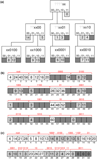
Figure 4: Trie algorithm for ranking, exemplified for $M=6$, $N=2$ and $R=2$. Here, we dispatch the least significant two bits, branch to the next node according to these, then shift and repeat. (a) Full trie, where white blocks represent branch nodes, grey boxes with numbers represent leaves. Suffix compression [Liang83PhD] is employed to reduce the trie size. (b) Linearized representation of the same trie for saving memory. (c) Packed representation to further reduce memory.

To this end, let us understand the fast ranking algorithm Fig. 3 as lookup in a tree index. For the case of $N=2$ particles in $M=6$ flavors and a chunk size of $R=2$ this is depicted in Fig. 4a: for any pattern $\alpha$, we start at the root node. We dispatch on the $R$ least significant bits $(\alpha_{1}\alpha_{0})$ and follow the $(\alpha_{1}\alpha_{0})$ branch to the next node. We then shift $\alpha$ by 2 bits to the right and repeat the procedure until we arrive at a leaf node, which contains the rank.

This procedure already suggests a generalization of the lookup for arbitrary quantum number sets: Elevating Fig. 4a to a data structure, we have constructed a trie (or prefix tree) [Briandais59, Knuth3]. A trie of radix $2^{R}$ for bit patterns of length $M$ is a search tree of height $\lceil M/R\rceil$ with a branching factor of $2^{R}$, i.e., each non-leaf node of the trie maintains an array of size $2^{R}$, which are pointers to descendant nodes. The leaf nodes instead represent the index $i$. (This is not exactly congruent with Fig. 4a, where we have omitted branches with only one possible path, a procedure known as suffix compression.) Tries maintain two important benefits of the staggered lookup algorithm: they process data in chunks of $R$ bits, thus only requiring $\lceil M/R\rceil$ lookups, and they replace branching by an indexing operation into an array of size $2^{R}$.

Tries, however, are not ideal in terms of memory locality and require significant memory overhead. To mitigate this, we can switch to a linearized representation [Liang83PhD], depicted in Fig. 4b: the trie is represented by a single contiguous array $(t_{0}\ldots t_{T-1})$, which is efficient since the trie is not mutated once created. Each node is then represented by an index $k$ in the array (the root node has index 0). For a branch node, the element $t_{k+r}$ contains the index of the child for the branch corresponding the $R$ active bits of the state being equal to $r$ (white boxes). For a leaf node, $t_{k}$ corresponds to the rank of the state (gray boxes).

We note that this structure is compatible with packing [Liang83PhD]: e.g., in Fig. 4, the branch node corresponding to $10_{2}$ does not have a child for $r=11_{2}$. We can thus omit the element for $r=11_{2}=3$. In general, a sequence of forbidden trailing descendants can be omitted. The same is true for forbidden descendants at the beginning: there, we omit the elements and move the index in the parent node forward by the number of elements deleted. For example, the node 0000 only allows $r=11_{2}$, so we can omit the first three elements. Consequently the index $t_{4}$, which is the corresponding element in node $00_{2}$, contains 5 rather than 8, reflecting the omission of 3 elements. As illustrated in Fig. 4c, packing thus significantly reduces the memory demand in cases where the trie is only sparsely populated. (Even more advanced packing strategies, where “holes” in the middle of the index are kept track of and filled by suitable nodes, are possible but beyond the scope of this paper.)

1:function $i=$ rank-trie($t,\alpha$)

2:     $i\leftarrow 0$

3:     for $i\in\{1,2,\ldots,\lceil M/R\rceil-1\}$ do

4:         $r\leftarrow\alpha\bmod 2^{R}$

5:         $i\leftarrow t_{i+r}$

6:         $\alpha\leftarrow\lfloor\alpha/2^{R}\rfloor$

7:     end for

8:     $i\leftarrow t_{i+\alpha}$

9:end function

Figure 5: Algorithm for ranking a state using linearized tries. Here $\bmod$ denotes the binary modulo operation; Fig. 4 exemplifies $t_{i}$.

Fig. 5 presents the algorithm for ranking a state using the linearized (and optionally packed) trie. Let us walk through the algorithm for, e.g., the trie in Fig. 4 and $\alpha=100100_{2}$: we start at the root with $i=0$. Since $r=\alpha\owedge 11_{2}=00_{2}=0$ and $t_{0}=4$, we move to $i=4$ and consider the next two bits of the state, $r=01_{2}$. Note that $t_{5}=8$, even though the data for node 0100 starts at index 9, as we have omitted the unused first child. Finally, we have $\alpha=10_{2}$ and the rank is given as $t_{8+2}=12$.

As with staggered lookup, we can now trade off memory overhead with lookup performance by adjusting the radix $R$. Unlike staggered lookup, the memory overhead now scales with the number $N_{s}$ of states in the sector, typically requiring $\mathcal{O}(fN_{s})$ space, where the overhead factor $f\geq 1$ depends on $R$ and the structure of the sector. In the example above, we have $f\approx 2$.

Let us add a remark on the trailing elements in the packed trie (Fig. 4c): we could omit those, since they are not pointing to any valid rank. However, including the full root node and the trailing elements of the last leaf node and setting the unused indices to zero ensures that the lookup procedure (Lines 5 and 8 in Fig. 5) will only ever access valid array indices, regardless of whether $\alpha$ is a valid state or not. This allows us to modify the algorithm in Fig. 5 to include a cheap check whether $\alpha$ is indeed a valid state in the sector: after the lookup, we simply verify that $t_{i}=\alpha$ by consulting the unrank lookup table.

Finally, let us turn back to our initial consideration, i.e., making the ranking algorithm suitable to conservation laws beyond the total number of particles (per spin sector). This is possible by simply eliminating all leaves and branches that do not fulfill a given conservation law. In practice, one starts by generating all states on the fly which fulfill particle number conservation in lexicographic order. Next, one filters out those states swhich do not satisfy additional conservation law. This iterator over state numbers is then fed into the trie generation routine, which can directly generate the packed trie.

V Numerical experiments

V.1 Ranking microbenchmark

To compare the established methods against one another, we first perform a microbenchmark focusing on lookup performance alone. For this, we consider $M=28$ spinorbitals and conserved total occupation $\hat{N}$ and analyze all sectors $N=1,\ldots,27$, which corresponds to ranking the combination set $C_{N}^{28}$.

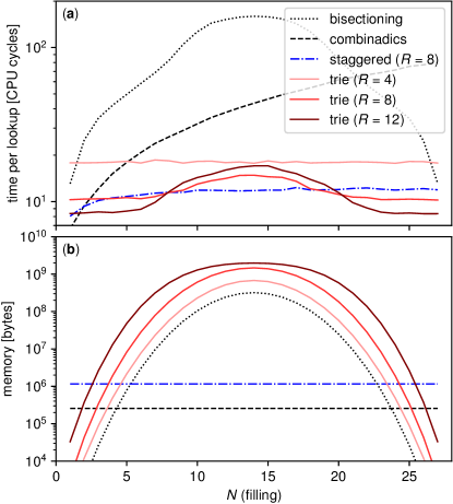
Figure 6: Lookup timings for combination with $M=28$ for sectors or varying filling $N\in\{1,\ldots,27\}$.

To this end, we implemented each ranking strategy—bisectioning, combination ranking, staggered lookup and trie lookup—as Julia [Julia] code and compiled with maximum optimization levels. We drew $10^{8}$ random states from each sector with replacement. We then ordered them by numerical value to simulate the situation that while the states generated in the application of Eq. (3) vary somewhat unpredictably, they are usually still ordered to some degree (omitting this ordering increases the cost of bisection search considerably and unfairly.) We then timed 20 iterations on a single AMD Ryzen-3600 CPU core.

The results are presented in Fig. 6. Panel (a) compares lookup times in terms of CPU cycles. We see that established methods (bisectioning and combinadics ranking) are generally slowest, except for the case of low filling: there, combinadics is most efficient since its scaling is with $N$ rather than $M$. Otherwise, we observe significant speedups for our improved algorithms, i.e., staggered and trie lookups. This speedup is particularly pronounced for close to half-filled sectors ($N\sim M/2$), since there the number of states is largest and thus cache misses become more and more of an issue for bisectioning. We further see that staggered lookup slightly outperforms tries for large sectors for the same $R$, since it is more economical in terms of cache demand. For a more sparsely populated sector (away from the half-filled case), we see that tries are slightly more efficient. In general, both trie and staggered lookups perform well, typically requiring around 10–15 CPU cycles per lookup.

Fig. 6(b) presents the corresponding memory demand for each index: here, the baseline is given by bisectioning, which requires an ordered list of all states $N_{s}$ in the sector. The trie indices add a radix-dependent overhead: for the half-filled case, we find an overhead factor $f\approx 2.11$ for $R=4$, $f\approx 4.58$ for $R=8$, and $f\approx 6.16$ for $R=12$. For the more sparsely populated cases $N=5$, one finds that the overhead increases more strongly: $f\approx 2.73$, $10.45$, and $61.06$ for $R=4,8$, and $12$, respectively. This is to be expected, as in the limit $R\to M$ we recover the inverse of the “sparseness” factor, $f\to 2^{M}/N_{s}$. Fortunately, the total memory demand of the index is still monotonously falling as we increase sparseness.

V.2 Hubbard chain

To examine the performance of ranking in a more realistic setting, let us study a special case of Eq. (1), namely a chain of $M/2$ Hubbard atoms:

$$H=-t\sum_{i=2}^{M/2}\sum_{\sigma}[\hat{c}^{\dagger}_{i\sigma}\hat{c}^{\mathchoice{\vphantom{\dagger}}{}{}{}}_{(i-1)\sigma}+\mathrm{h.c.]}+U\sum_{i=1}^{M/2}\hat{c}^{\dagger}_{i\uparrow}\hat{c}^{\dagger}_{i\downarrow}\hat{c}^{\mathchoice{\vphantom{\dagger}}{}{}{}}_{i\downarrow}\hat{c}^{\mathchoice{\vphantom{\dagger}}{}{}{}}_{i\uparrow},$$ (16)

where the sum over spins $\sigma$ runs over $\{\uparrow,\downarrow\}$. We are interested in computing the lowest energy eigenvalue by constructing the Krylov subspace given sector $N,S_{z}$ (cf. Eq. 12) using the Lanczos algorithm, on-the-fly evaluation (3). We implemented these techniques in Julia and ran the calculations in parallel on six AMD Ryzen-3600 CPU cores on the same node.

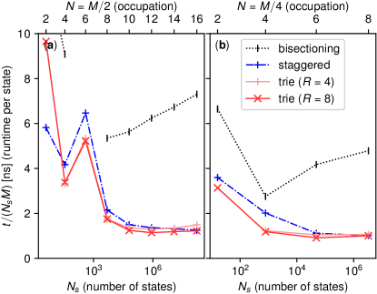
Figure 7: Runtime of different ranking strategies when performing a vector–matrix multiplication $H|\psi\rangle$ with (16) for two sectors: (a) $N=M/2$ and $S_{z}=0$ for $M=4,8,\ldots,32$ and (b) $N=M/4$ and $S_{z}=0$ for $M=8,16,24,32$. We plot the average runtime per state over the number $N_{s}$ of states in the sector (bottom axis) and the occupation $N$ (top axis), respectively.

Fig. 7 presents the average runtime for a single matrix–vector multiplication $H|\psi\rangle$ per state, i.e., the total runtime divided by the number $N_{s}$ of states in the sector as well as divided by $M$, in units of nanoseconds. We see that both our ranking techniques, staggered and trie lookup, improve substantially on the state-of-the-art bisectioning, achieving an around three-fold speed-up.

We note that the timings in Fig. 7 not only include rankings. Indeed, Eq. (3) suggests the following, rather crude, estimate for the total runtime:

$$t\approx N_{s}N_{t}(t_{\mathrm{rank}}+t_{\mathrm{apply}}+t_{\mathrm{FMA}}+t_{\mathrm{mem}}),$$ (17)

where $N_{t}$ is the number of non-branching terms (in our case, $N_{t}=3M/2$), $t_{\mathrm{rank}}$ is the time needed for ranking states, $t_{\mathrm{apply}}$ is the time needed for computing the bit operations when applying $T$ in Eq. (3), $t_{\mathrm{FMA}}$ is the time needed for multiplying with the corresponding element of $\psi$ and accumulating the result, and $t_{\mathrm{mem}}$ is the time for accessing the corresponding component of $\psi$. Disentangling the constituent times is difficult, but profiling information suggests that around 1/3 of runtime is spent on ranking in the case of staggered and trie lookup. This is consistent with Fig. 6(a), where we only observe a moderate increase of $t$ with $N$ even though one expects linear scaling of $t_{\mathrm{rank}}$. In contrast, for the bisectioning lookup the ranking times completely dominate the computation.

Since trie and staggered lookup scale with $M$ rather than $N$, the half-filled case $N=M/2$ in Fig. 6(a) is most favorable for these algorithm. To study a more sparse setting, Fig. 6(b) presents timings for the quarter-filled case $N=M/4$. There, bisectioning, which scales with $\min(N,M-N)$, cf. Fig. 5, improves compared to staggered and trie lookup. However, we still observe an about four-fold speed-up by switching to the improved ranking algorithms.

Let us finally note that the differences within the improved algorithms are minor, consistent with the ranking microbenchmark in Sec. V.1. Interestingly, even though trie lookup with $R=8$ consistently outperforms $R=4$ in the microbenchmark, the two algorithms have similar performance in the benchmark Fig. 6. This may be due to the fact that $R=8$ has a significantly larger memory footprints which becomes more relevant for the full algorithm, so the cache misses may balance out the speed benefit. (Cache pressure is expected to be higher in this benchmark due to the manipulation of the state vectors.)

V.3 Hubbard ring

To showcase trie ranking (Sec. IV), we choose a system and a set of quantum numbers where staggered lookup is not possible. To do so, we consider again a one-dimensional system of $M/2$ Hubbard atoms, but with periodic boundary conditions:

$$H=-2t\sum_{k\sigma}\cos(k)\hat{c}^{\dagger}_{k\sigma}\hat{c}^{\mathchoice{\vphantom{\dagger}}{}{}{}}_{k\sigma}+U\sum_{kk^{\prime}q}\hat{c}^{\dagger}_{(k+q)\uparrow}\hat{c}^{\dagger}_{(k^{\prime}-q)\downarrow}\hat{c}^{\mathchoice{\vphantom{\dagger}}{}{}{}}_{k\downarrow}\hat{c}^{\mathchoice{\vphantom{\dagger}}{}{}{}}_{k^{\prime}\uparrow},$$ (18)

where $\sigma\in\{\uparrow,\downarrow\}$, $k\in\{0,4\tfrac{\pi}{M},8\tfrac{\pi}{M},\ldots,(2M-2)\tfrac{\pi}{M}\}$ and we enforce periodic boundary conditions by identifying $\hat{c}^{\mathchoice{\vphantom{\dagger}}{}{}{}}_{k\sigma}\equiv\hat{c}^{\mathchoice{\vphantom{\dagger}}{}{}{}}_{(k+2\pi)\sigma}$.

Let us note that $H$ in the momentum basis (18) is significantly less compact than the real-space formulation, cf. Eq. (16), since the Hubbard interaction generates $\mathcal{O}(M^{3})$ terms. For this reason, such symmetries are usually taken into account implicitly in ED codes by generating a set of “representative” states in the real-space basis and then symmetrizing the result to obtain the corresponding momentum state [Lin90SublatticeCoding]. However, there are other quantum numbers, such as orbital parity in quantum impurity models (also known as the PS quantum number [Parragh12PS]), which can be directly expressed in the real-space occupation number basis.

These caveats nonwithstanding, the momentum basis admits a further quantum number, the total crystal momentum:

$$K_{\mathrm{tot}}=\sum_{k\sigma}k\hat{c}^{\dagger}_{k\sigma}\hat{c}^{\mathchoice{\vphantom{\dagger}}{}{}{}}_{k\sigma}\mod 2\pi,$$ (19)

which commutes with both the Hamiltonian and the occupation number basis and can thus be readily used to lower the block size. Therefore, it provides a benchmark for trie rankings vs. established bisectioning methods.

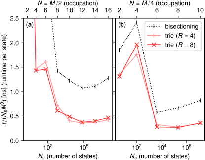
Figure 8: Runtime of different ranking strategies when performing a vector–matrix multiplication $H|\psi\rangle$ with (18) for two sectors: (a) $N=M/2$, $S_{z,\mathrm{tot}}=0$, and $K_{\mathrm{tot}}=0$ for $M=4,8,\ldots,32$ and (b) $N=M/4$, $S_{z}=0$ and $K_{\mathrm{tot}}=0$ for $M=8,16,\ldots,40$. We plot the average runtime per state over the number $N_{s}$ of states in the sector (bottom axis) and the occupation $N$ (top axis), respectively.

Fig. 8 again presents the average runtime for a single matrix–vector multiplication $H|\psi\rangle$ per state, i.e., the total runtime divided by the number $N_{s}$ of states in units of nanoseconds. Instead of by $M^{-1}$ as in Fig. 7, the runtime is scaled with $M^{-3}$, since that is the scaling of the number of terms in Eq. (18). We see that the speed-up of trie lookup vs. bisection is milder here than in Sec. V.2. We can attribute this to the greater “sparseness” of states in the space of $M$-bits, which means that tries have to process more bits per state. However, the benefit is still substantial, with a two- to three-fold improvement in runtime observed.

Notably, instead of plateau for trie-based ranking in Fig. 7, we see an uptick in runtime for large $M$ in Fig. 8. This may be indicative of growing cache pressure in this cases due to the memory footprint of the trie.

VI Conclusions and outlook

We have removed a computational bottleneck of exact many-fermion calculations by speeding up the ranking of states, thereby providing an efficient mapping between indices of state in the full Fock space and in the block corresponding to a set of quantum numbers. For the common case of conserved particle number, the state-of-the-art combinadics algorithm present in many ED algorithms can be modified to yield considerable ranking speed-ups at negligible overhead with a staggered lookup. For more complictated quantum number combinations, the state-of-the-art bisectioning algorithm can be replaced by a trie lookup, which has a similar scaling with memory but a much-improved performance. Thanks to these improvements, ranking is no longer the bottleneck of the ED code.

With these optimizations, we expect exact diagonalization to stay competitive as, e.g., a solver for quantum impurity models [DMFT] in cases where the quantum Monte Carlo techniques encounter a significant sign problem or where high numerical accuracy is required for, e.g., analytic continuation [Otsuki17, Nevanlinna].

Trie ranking is also applicable to non-Abelian symmetries [Lin90SublatticeCoding] leveraged in spin systems, where instead of ranking states in a quantum number sector we are ranking representatives of a symmetry orbit within a symmetry sector. Combining trie lookup and sublattice coding techniques [Lin90SublatticeCoding, Lauchli18] seems particularly promising, as sublattice coding reduces the size and scaling of the states which have to be ranked, which should make the memory overhead associated with tries less problematic also for large systems.

An intriguing challenge for trie rankings are selected CI techniques [Huron73] as well as related Monte Carlo approaches [FCIQMC, Jaklic94], which restrict FullCI to a subset of states in the Fock space. These techniques optimize the set, either stochastically or deterministically, by minimizing the ground state energy, which means the set to be ranked cannot be static. This “dynamic ranking” makes the use of linearized and packed tries impractical, so ranking based on hash tables could be competitive.

A unit-tested Julia implementation of the techniques outlined here is available from the authors upon reasonable request and forthcoming as an open-source package.

Appendix A Non-branching term rules

For completeness, we show here how to construct general rules for non-branching terms and arbitrary products thereof. Most of this material is well-known, but the product rule has to the best of our knowlege not been stated in this general form.

We begin by restating Eq. (3) in a slightly altered form: let $T$ be an arbitrary product of creation and annihilation operators (not necessarily normal-ordered) with a scalar prefactor. Then there exists a tuple ($v,m,l,r,x,s$) of numbers such that the application of $T$ on any basis state $|\alpha\rangle$ in the occupation number basis is:

$$T|\alpha\rangle =v\delta_{\alpha\owedge m,r}(-1)^{h(\alpha\owedge s)}|\alpha\oplus x\rangle,$$ (20)

$$\langle\alpha|T =v\delta_{\alpha\owedge m,l}(-1)^{h(\alpha\owedge s)}\langle\alpha\oplus x|,$$ (21)

where $\owedge$ denotes bitwise and, $\oplus$ denotes bitwise xor, and $h$ is the Hamming weight, i.e., the number of set bits. (We have added an element $l$ for later convenience.)

By way of a proof, we will offer an algorithm to construct $(v,m,l,r,x,s)$. Let us start with the “building blocks”, the annihilation operators $\hat{c}^{\mathchoice{\vphantom{\dagger}}{}{}{}}_{i}$. By comparing Eq. (20) with Eq. (2), one finds that:

$$v =1, m =2^{i},$$ (22a)

$$l =0, r =2^{i},$$ (22b)

$$x =2^{i}, s =2^{i}-1.$$ (22c)

The values for corresponding creation operator $\hat{c}^{\dagger}_{i}$ are obtained by simply exchanging $l$ and $r$. (The same is true for the transpose of any other term.)

1:function $t=$ mul($t_{a},t_{b}$)

2:     $(v_{a},m_{a},l_{a},r_{a},x_{a},s_{a})\leftarrow t_{a}$

3:     $(v_{b},m_{b},l_{b},r_{b},x_{b},s_{b})\leftarrow t_{b}$

4:     if $(r_{a}\oplus l_{b})\owedge m_{a}\owedge m_{b}\neq 0$ then

5:         $v\leftarrow 0$

6:     else

7:         $v\leftarrow v_{a}v_{b}$

8:     end if

9:     $m\leftarrow m_{a}\ovee m_{b}$

10:     $r\leftarrow r_{b}\ovee(r_{a}\owedge\neg m_{b})$

11:     $l\leftarrow l_{a}\ovee(l_{b}\owedge\neg m_{a})$

12:     $x\leftarrow l\oplus r$

13:     $s\leftarrow s_{a}\oplus s_{b}$

14:     $s\leftarrow s\owedge\neg m$

15:     $z\leftarrow r$

16:     $p\leftarrow z\owedge s_{b}$

17:     $z\leftarrow z\oplus x_{b}$

18:     $p\leftarrow p\oplus(z\owedge s_{a})$

19:     $v\leftarrow v(-1)^{h(p)}$

20:     $t\leftarrow(v,m,l,r,x,s)$

21:end function

Figure 9: Fast algorithm for constructing the tuple $t$ for on-the-fly multiplication for a product $T=T_{a}T_{b}$, where the factors $T_{a}$ and $T_{b}$ are encoded by tuples $t_{a}$ and $t_{b}$, respectively. Here, $\owedge$ denotes bitwise and, $\ovee$ denotes bitwise or, $\oplus$ denotes bitwise xor, $\neg$ denotes bitwise not, and $h(x)$ counts the number of set bits in $x$.

We can now understand the role of each of the elements in the tuple: $m$ is the bitmask, with bit $i$ set whenever there is any operator in $T$ with flavor $i$. $r$ is the “demands” of $T$ on its right side, i.e., for any flavor in $m$, the state $\alpha$ must have the same occupation as $r$ does whenever $T$ is applied from the left or the result will be zero. The same holds for $l$ when $T$ is applied from the right. The tuple $(v,m,l,r)$ is enough to encode the full term ($m$ can be omitted if normal-ordering is imposed), but for performance reasons it is advantageous to store two more fields: set bits in $x$ correspond to those flavors which will be changed by $T$. Finally, $s$ is the sign mask, which encodes the anticommutativity rules: whenever $T$ is applied to $\alpha$ any flavor in $\alpha$ that is also in $s$ will cause the result to flip sign.

To complete the proof, we need to construct the product $T=T_{a}T_{b}$ of two terms. We present this algorithm in Fig. 9. There, $t=(v,m,l,r,x,s)$ is the desired result, tuple for $T$. The inputs are the tuple $t_{a}=(v_{a},m_{a},l_{a},r_{a},x_{a},s_{a})$ for $T_{a}$ and $t_{b}=(v_{b},m_{b},l_{b},r_{b},x_{b},s_{b})$ for $T_{b}$.

Lines 4–8 check the Pauli principle. This is relatively easy: let us denote by $|\psi\rangle$ the “intermediate” state in the application of $T$, i.e., $T|\alpha\rangle=T_{a}|\psi\rangle$. $r_{a}$ and $l_{b}$ are then “demands” of $T_{a}$ and $T_{b}$, respectively, on $\psi$, each each confined to their mask. This means we simply have to fulfill both demands whenever the masks intersect $m_{a}\owedge m_{b}$. When the demands are not fulfilled, the Pauli principle is violated and the value $v$ of the term is set to zero (line 7), otherwise it is—for now—simply the product of both scalars (line 5).

Line 9–14 deal with the actual composition of the two terms. Firstly, in line 9, we construct the mask $m$ as union of the individual masks, since the operator flavors in the product are just the union of the operators in each factor. For the right outer state $r$, $r_{b}$ takes precedence whenever $m_{b}$ is set, otherwise, the other term can make demands $r_{a}$ (line 10). For the left outer state $l$, we make a similar argument (line 11). The change mask $x$ is given simply as the symmetric bit difference between left and right (line 12).

The sign mask $s$ is at first set as the simple exclusive or of the individual masks (line 13), however, there is a complication: the creation and annihilation operators alter the state $\alpha$, so each flavor in $m$ is “locked” in place by $T$. This means we need to exclude any flavor from the sign mask $s$ that is also present in $m$ (line 14).

The term $T^{\prime}$ we have constructed so far is almost equal to $T=T_{a}T_{b}$, however, it may still deviate from $T$ by a sign due to the reordering of creators and annihilators encoded in the tuple $t$. Instead of keeping track of these permutations explicitly, we use a computationally appealing shortcut: we simply compare the effects of $T_{a}T_{b}|\alpha\rangle$ and $T^{\prime}|\alpha\rangle$ for a state where $T|\alpha\rangle\neq 0$. One such state is, by construction, $|r\rangle$. Lines 15–18 compute Eq. (20) for $T_{a}T_{b}|r\rangle$ and keep track of the relevant sign masks overlaps in $p$. Any deviation between $T$ and $T^{\prime}$ is then absorbed into $v$ (line 19) and the algorithm is complete.

We note that the algorithm in Fig. 9 does not only prove that a tuple for on-the-fly application exists, it also offers an extremely fast way to compute products of terms on modern machines, as it relies exclusively on bit operations.