Critical percolation threshold restricts late-summer Arctic sea ice melt pond coverage

Abstract

During the summer, vast regions of Arctic sea ice are covered by meltwater ponds that significantly lower the ice reflectivity and accelerate melting. Ponds develop over the melt season through an initial rapid growth stage followed by drainage through macroscopic holes. Recent analysis of melt pond photographs indicates that late-summer ponds exist near the critical percolation threshold, a special pond coverage fraction below which the ponds are largely disconnected and above which they are highly connected. Here, we show that the percolation threshold, a statistical property of ice topography, constrains pond evolution due to pond drainage through macroscopic holes. We show that it sets the approximate upper limit and scales pond coverage throughout its evolution after the beginning of drainage. Furthermore, we show that the rescaled pond coverage during drainage is a universal function of a single non-dimensional parameter, $\eta$, roughly interpreted as the number of drainage holes per characteristic area of the surface. This universal curve B6allows us to formulate an equation for pond coverage time-evolution during and after pond drainage that captures the dependence on environmental parameters and is supported by observations on undeformed first-year ice. B18This equation reveals that pond coverage is highly sensitive to environmental parameters, suggesting that modeling uncertainties could be reduced by more directly parameterizing the ponds’ natural parameter, $\eta$. Our work uncovers previously unrecognized constraints on melt pond physics and places ponds within a broader context of phase transitions and critical phenomena. Therefore, it holds promise for improving ice-albedo parameterizations in large-scale models.

I Introduction

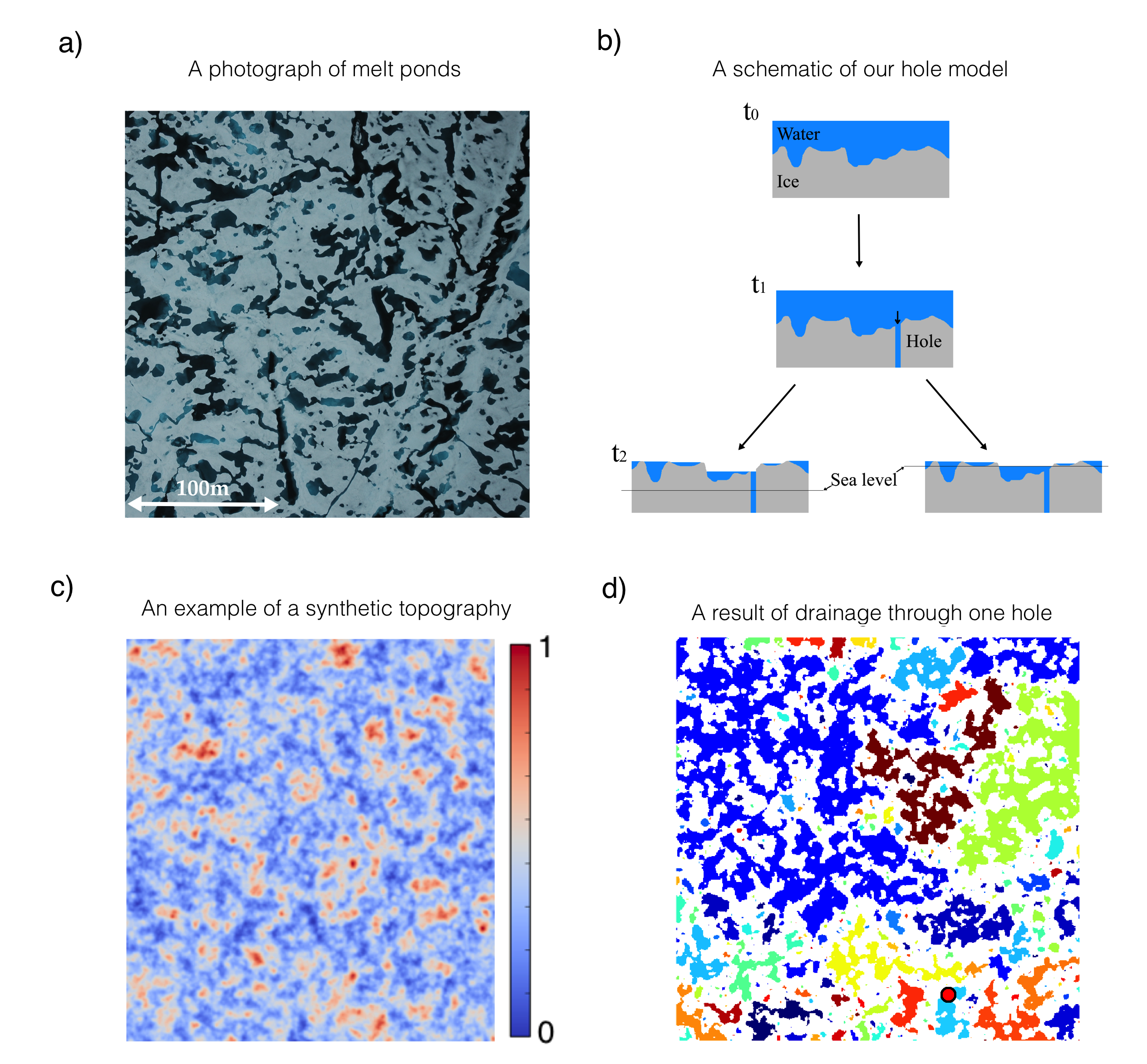
Figure 1: a) A photograph of melt ponds taken during the 2005 HOTRAX mission. b) A sketch of the hole drainage model. The model begins with an ice surface, a large fraction of which is flooded. A hole opens at a random location on the ice and starts draining the ponds that are connected to it. As the drainage progresses, some regions of the ice become disconnected from the hole and can no longer drain through it. Drainage stops when either the hole is exposed to the atmosphere or when the water level of the pond connected to the hole reaches sea level. c) An example of randomly generated “snow dune” topography. Red colors stand for topographic highs while blue colors stand for topographic lows. The upper bound on the scale bar, here set to 1, is arbitrary. This panel is taken from Popović et al. (2020). d) Ponds after drainage on the topography in panel c) through the hole marked with a red dot. Different colors correspond to distinct ponds.

Arctic sea ice covers a vast area of nearly 15 million square kilometers at its peak annual extent. It sculpts the Arctic environment, supports its ecosystem, and presents a significant obstacle to trade (Perovich and Richter-Menge, 2009). In recent years, sea ice has been rapidly disappearing at a rate underestimated by most climate models (Stroeve et al., 2007). These climate models cannot resolve processes on scales smaller than tens of kilometers, and the disagreement with observations is largely attributed to such unresolved processes (Holland and Curry, 1999). A notable example of a small-scale process contributing to the uncertainty of the large-scale predictions is meter-sized melt ponds that form on the ice surface during summer (Fig. 1a). Melt ponds absorb roughly twice as much solar radiation as surrounding bare ice, which significantly accelerates ice melt (Perovich, 1996). Several works have shown the crucial role ponds play in predicting the state of sea ice (Schröder et al., 2014; Holland et al., 2012). For example, Schröder et al. (2014) demonstrated that the summer sea ice minimum extent can be accurately predicted based only on the spring melt pond extent. Currently, the most common tactic for modeling melt ponds is to try to represent as many of the physical processes that contribute to pond evolution as realistically and as comprehensively as possible (Lüthje et al., 2006; Flocco and Feltham, 2007; Skyllingstad et al., 2009, 2015). Although such models capture many properties of melt pond evolution, it is unclear how assumptions and details of these complex models might change in a warmer climate. This suggests an opportunity for modeling based on universal properties of sea ice that will likely remain unchanged in a warmer climate.

Melt ponds develop in several stages that depend on the microstructure of the underlying ice (Polashenski et al., 2012; Landy et al., 2014; Polashenski et al., 2017). As sea ice forms from freezing salty water, brine pockets and channels fill the ice interior (Perovich and Gow, 1996; Cole and Shapiro, 1998; Golden et al., 2007). When the summer melt season begins, fresh water from melting snow penetrates into the cold ice interior through these brine structures, freezes, and thereby plugs the pathways connecting the ice surface to the ocean. The lack of pathways to the ocean allows water to collect in ponds at the top of the ice (Polashenski et al., 2017). Since the ice is relatively flat, ponds grow rapidly during this time, and sometimes end up covering the majority of the ice surface at their peak. This rapid growth stage is usually known as “stage I” of pond evolution. Later, as ice warms, some of the frozen freshwater plugs melt, once again opening the pathways to the ocean and draining the ponds. As relatively warm pond water flows through these channels, it can expand them into large holes that can drain very large areas in a matter of hours (Polashenski et al., 2012). More such holes open with time, and, over the course of several days, pond coverage falls to its minimum. The period during which ponds that are above sea level drain to reduce their hydraulic head is known as “stage II” of pond evolution. Afterwards, the remaining ponds correspond to those regions of ice surface that are below sea level. From this point, pond coverage slowly grows as the ice thins and more of the ice surface falls below sea level. This is known as “stage III” of pond evolution. Observations show that during stage II, meltwater is mainly drained through large holes, while during stage III it is mostly drained through microscopic pathways in the ice (Polashenski et al., 2012).

Recently, in Popović et al. (2018), we analyzed photographs of melt ponds and showed that the post-drainage melt pond geometry can be accurately described by a purely geometrical model where ponds are represented as voids that surround randomly sized and placed circles, which can be loosely interpreted as snow dunes. Surprisingly, we found that in order to match various statistics derived from images of late-summer ponds, the fraction of the surface covered by voids had to be tuned to a special value: the percolation threshold. The concept of a percolation threshold coverage fraction, $p_{c}$, was developed in physics and applied to modeling diverse phenomena ranging from electrical transport in disordered media to turbulence (Isichenko, 1992). In the idealized setting of an infinite plane covered randomly by objects that can overlap to form larger clusters, the percolation threshold is the coverage fraction below which only finite connected clusters can exist and above which an infinite cluster that spans the domain forms. Exactly at $p_{c}$, connected clusters of all sizes exist, and the system becomes scale-invariant. Close to this threshold, percolation models exhibit universality (Goldenfeld, 1992) which means that much of the system behavior does not depend on details such as, for example, the shape of connecting objects. Generally speaking, universality is often observed near the critical point of continuous phase transitions. Thus, for example, universality allows both the magnetic phase transition and the phase transition of fluids near the critical point to be accurately described by the idealized Ising model (Goldenfeld, 1992; Nishimori and Ortiz, 2010).

Our observation that late-summer ponds seem to be organized close to the percolation threshold presents a puzzle and suggests that there is a mechanism driving the ponds to this threshold. Here, we show that drainage through large holes can account for this observation. Specifically, we develop an idealized model of pond drainage through large holes to show how this mechanism drives melt pond evolution to lie below the percolation threshold. We then use this model to formulate a pond fraction evolution equation that reveals the connections between the pond evolution and measurable physical parameters. B2Even though our hole drainage model explicitly represents the drainage stage (stage II), we show that it can also be used to understand elements of pond evolution during stage III. By clarifying the relation of pond coverage to the percolation threshold, we place melt pond formation within the broader context of critical phenomena and phase transitions.

A4Our approach to modeling melt ponds here is very different from using a typical pond-resolving model. Such models solve pond and ice evolution on a grid, often in 3 dimensions, parameterizing the sub-grid scale processes that cannot be explicitly resolved. For example, in a recent attempt, Skyllingstad et al. (2015) solved a 3d model of pond evolution coupled with ice thermal evolution, assuming that ponds drain through the bulk of the ice, and allowing the possibility for an impermeable ice layer to form. Their model physics allowed for all stages of pond evolution to emerge naturally as the ice permeability evolves, but, to match the measured pond evolution, the ice permeability had to be tuned several orders of magnitude below the observed value. In this paper, for the first time, we explicitly model pond drainage through large holes and, as a result, we are able to match the observations using realistic physical parameters. Moreover, we use an explicitly solvable model that exhibits universality, which makes it numerically inexpensive and easily interpreted.

This paper is organized as follows: First we formulate a model of drainage through large holes. Next, we use this model to explain why the ponds organize around the percolation threshold. After this, we show that the drainage process is in fact universal. In the two following sections, we use universality to formulate an equation for pond coverage evolution that approximately solves the hole model. Next, we show that our results are consistent with observations. Then, we discuss the dependence of pond coverage evolution on physical parameters and the challenges of pond modeling and, finally, we conclude with a summary of our results. All of the parameters used in the paper are summarized in table 2. We summarize technical details required to reproduce the results of the paper in the Supporting Information (SI).

II The hole model

To investigate pond drainage through macroscopic holes, we created a simple model of pond drainage, sketched in Fig. 1b and explained in detail in SI section LABEL:sec:model. We discuss the physics of hole formation later, in section V. B2.1To mimic the conditions at the end of stage I of pond evolution, we start with a random synthetic two-dimensional ice surface, a large fraction of which is covered by water. B6.2We are assuming that variations in ice topography are initially much smaller than freeboard height (mean height above sea level), such that no regions of the ice are initially below sea level. Such a configuration is consistent with conditions on undeformed first-year ice. The ice topography can change over the course of the melt season, as preferential melting of ponded ice alters the topography. A hole opens at a random location on the ice surface and drains water from all of the ponds it is connected to. As drainage through this hole progresses, some parts of the surface can become disconnected from the hole and can no longer drain through it. Drainage stops when either the hole is exposed to the atmosphere or when the pond connected to the hole reaches sea level. As water is lost from the ice surface, the ice floats up to maintain hydrostatic balance. Hydrostatic balance depends on ice thickness, which can decrease over time. Since ponded ice melts faster than bare ice, we evolve the topography by preferentially melting ponded regions. We are assuming that this melt occurs much slower than drainage through a hole. A11B1 We are also assuming that the topography only changes due to albedo differences between bare and ponded ice so that channels that connect ponds cannot form as the ponds drain. Later, more holes open on the ice surface and the process continues until all the ponds are at sea level.

B1.2In practice, we implemented our model on a square grid, typically $500\times 500$ grid points in size, with boundaries that we regard as rigid walls over which ponds cannot spill. We initiated the model by randomly generating a topography according to one of the schemes described in SI section LABEL:sec:topos and setting an initial water level, typically so that 100% of the surface is water-covered. During each simulation run, we tracked the ice height above sea level and the water level at each grid point as well as a global variable, $\theta$, loosely interpreted as ice temperature. $\theta$ increases at a fixed rate and determines where the holes open - to each grid point, we assign a critical value, $\theta_{0}$, drawn independently from a normal distribution, so that a hole opens at that grid point when $\theta>\theta_{0}$. Ice thickness, which controls the height of the freeboard, decreases at a constant rate $\text{d}H/\text{d}t$, which we take to be an independent model parameter, separate from the surface melt rate. We consider both simulations with $\text{d}H/\text{d}t=0$ and with $|\text{d}H/\text{d}t|>0$. We simulate pond and ice evolution iteratively - 1) first, we update $\theta$ to find grid points where the new holes open, 2) then we drain the ponds through these holes by incrementally decreasing the water level, at each step updating the ponds connected to the holes until either the holes emerge above the pond surface or ponds fall to sea level, 3) next, we update the surface topography by preferentially melting ponded regions, and 4) finally, we update ice thickness and impose hydrostatic balance. We repeat these steps until $\theta$ is high enough so that all grid points have a hole in them. We describe this model in more detail and carefully consider all of the model assumptions in SI sections LABEL:sec:model and LABEL:sec:assumptions. Code for this model is archived in Popović (2020) and is also available at https://github.com/PedjaPopovic/hole-model.

Ice topography determines how the ponds will drain. As we will show, the effects of topography on pond coverage can be summarized with only a few parameters. Importantly, though, for our analysis to apply, ice topography has to be well-described by a single length scale, $l_{0}$, defined, for example, as the autocorrelation length. In the case of melt ponds, $l_{0}$ would be determined by the typical size of snow dunes. By only considering single-scaled topographies, we are restricting our analysis to flat regions of the ice away from large-scale features such as the ridges. A10 As we mentioned in the introduction, an especially important property of the surface is its percolation threshold, $p_{c}$. We estimate $p_{c}$ for a given topography as the coverage fraction at which a connected “pond” that spans the domain first appears as we incrementally raise the “water level” (a horizontal plane that cuts through the topography, see SI section LABEL:sec:topos for details). Motivated by the void model of Popović et al. (2018) where ponds surround circular “snow dunes,” in Popović et al. (2020) we developed a “snow dune” model of the ice topography generated by summing randomly placed mounds of Gaussian form, each with a randomly chosen horizontal scale and a height proportional to that scale. There, we showed that this topography reproduces the statistical properties of the pre-melt snow surface highly accurately. An example of this surface is shown in Fig. 1c and a typical configuration of ponds after drainage through one hole on this surface is shown in Fig. 1d. However, our analysis applies to any random surface with a single characteristic scale, and we also show the results for other topography types. We discuss all of these topographies in SI section LABEL:sec:topos.

III The origin of the percolation threshold in melt ponds

Figure 2a shows the pond coverage fraction, $p$, as a function of the number of open holes, $N$, in the hole model if we assume ice does not melt. Figure 2a provides insight into the mechanism for pond coverage being organized close to the percolation threshold, $p_{c}$. Specifically, we can see that the first several holes drain the entire ice surface from $p=1$ to $p\approx p_{c}$, while it takes on the order of $10^{5}$ more holes to drain the rest of the surface. In these simulations, the total number of pixels was $N_{0}\approx 2.5\times 10^{5}$, so to fully drain the surface, a hole needed to exist on nearly every pixel. This resembles the opening of microscopic pathways in real ice, and explains why the transition from stage II to stage III is also marked with a transition from drainage through large holes to drainage through microscopic pathways. B13This result was robust - we ran multiple simulations on three kinds of topographies and in each case the first several holes were able to drain ponds to below $p_{c}$, while the remainder of the drainage curves were robust against the randomness in our model.

We can now understand why the initial drainage is so abrupt and leads to pond coverage close to the percolation threshold. If pond coverage is above the threshold, then a large fraction of the surface is connected and a single hole can drain a vast area. On the other hand, if pond coverage is below the threshold, then ponds become disconnected and holes can drain ponds only incrementally. To explain why ponds remain close to the percolation threshold as more holes open, we need to include the fact that ponded ice melts faster than bare ice. In this case, the topographic variations that determine the pond patterns amplify over time, so that percolation pond patterns can be preserved if ponded ice melts sufficiently fast compared to bare ice.

The percolation threshold is a statistical property of the ice surface. As such, it does not depend on many of the details of the topography. Importantly, it does not typically depend on dimensional properties such as the mean height or roughness (standard deviation), but rather on generic statistical properties of the surface (Weinrib, 1982). For example, any surface that has a height distribution with a point of symmetry (e.g., a Gaussian), will have $p_{c}=0.5$ (Zallen and Scher, 1971).A12 Non-symmetric surfaces have a $p_{c}$ that deviates from 0.5, but our experiments on non-symmetric “snow dune” and Rayleigh topographies suggest that these deviations are typically not very large (see SI section LABEL:sec:topos). This means that the percolation threshold for real ice can likely be accurately estimated using an appropriate statistical model of ice topography.A11.2 We note that if channels that connect ponds form in a significant number as the ponds drain, statistical properties of the topography may change over the course of pond drainage, thereby lowering the value of the percolation threshold.

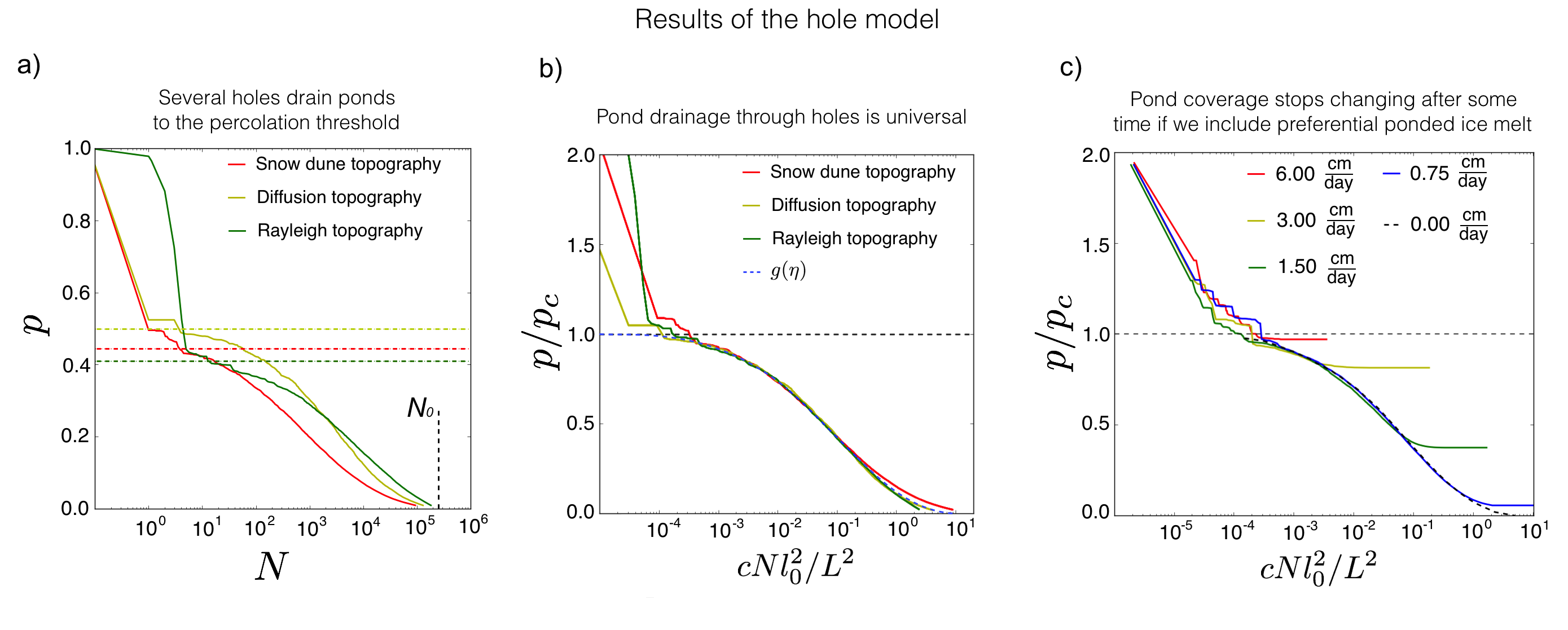
Figure 2: a) Semi-log plot of pond coverage fraction as a function of the number of open holes for three different topography types and no ice melt. Percolation thresholds for each of the three topographies are shown as horizontal dashed lines. The vertical dashed line marks the total number of pixels in these simulations. The simulations start at $N=0$ and $p=1$ which cannot be shown due to the logarithmic scale, so, for visual clarity, we artificially place the origin at $N=0.1$. b) A plot of rescaled pond coverage, $\Pi\equiv p/p_{c}$, as a function of rescaled number of holes, $\eta\equiv cNl_{0}^{2}/L^{2}$ for the three surfaces in panel a. The horizontal dashed line marks the percolation threshold, $\Pi=1$. Following initial drainage above the percolation threshold, all three curves fall approximately on a universal function, $g(\eta)$, marked with a dashed blue line. c) Rescaled pond coverage, $\Pi$, as a function of rescaled number of holes, $\eta$, now with preferential ponded ice melt, for different rates of ponded ice melt relative to bare ice melt, $\text{d}h_{\text{diff}}/\text{d}t$. Ice thinning rate is kept at 0, i.e., $\text{d}H/\text{d}t=0$. The horizontal dashed line has the same meaning as in panel b.

IV Universality of drainage through holes

The curves for drainage on different topographies shown in Fig. 2a all appear different. However, by rescaling $p$ and $N$, we can collapse these curves onto a single universal curve (Fig. 2b). The appropriate rescaling is

$$p \rightarrow \Pi\equiv\frac{p}{p_{c}}$$ (1)

$$N \rightarrow \eta\equiv cN\frac{l_{0}^{2}}{L^{2}}\text{ , }$$ (2)

where $L$ is the size of the domain and $c$ is a non-dimensional number of order unity that, like $p_{c}$, depends on the type of the topography but not on its dimensional properties such as mean height or roughness. B53Below we show that $c$ can be defined using a theoretical curve that arises from the general percolation theory. A factor $L^{2}/l_{0}^{2}$ in the parameter $\eta$ is approximately the number of ponds of size $l_{0}$ within the domain of size $L$. Therefore, the parameter $\eta$ represents, approximately, the number of open holes per pond of size $l_{0}$. As we can see in Fig. 2b, the surface is significantly drained when $\eta$ is of the order one, meaning that it takes about one hole per pond to drain the surface. After this rescaling, drainage on all surfaces follows a universal law

$$\Pi=g(\eta)\text{ . }$$ (3)

Pond coverage in our model falls on this universal curve after the first several holes have drained the ponds to the percolation threshold. For a general discussion on universality see Goldenfeld (1992).

B3The universality of the curve $g(\eta)$ is a consequence of the universality of the percolation model near $p_{c}$. In SI section LABEL:sec:g, we use this fact to motivate the form of $g(\eta)$. In particular, we define a correlation function for ponds, $G(l)$, as the probability that two randomly chosen points on the surface, separated by a distance $l$, are both located on the same pond. With this definition, the integral of $G(l)$ is proportional to the fraction of the surface connected to a randomly located hole, and, so, can be related to an average decrease in pond coverage per hole. The universality of pond drainage then arises from the fact that, close to the percolation threshold, $G(l)$ has the same form for all models within the percolation universality class. In SI section LABEL:sec:g, we use this line of reasoning to show that $g$ is approximately a solution to an ordinary differential equation

$$\frac{\text{d}g}{\text{d}\eta}=-g^{2}(1-g)^{-19/18}\text{ . }$$ (4)

This reasoning only holds near $p_{c}$, so, when $\Pi$ deviates significantly from 1, the universality breaks down, which we can see in the hole model with the slight deviation among the curves at low pond coverage in Fig. 2b. We use Eq. 4 to specify the constant $c$ in the parameter $\eta$. We chose $c$ so that the simulated curves $\Pi=g(\eta)$ best correspond to Eq. 4. All tested topographies yielded a similar scaling factor, $c$, so this constant had only a small effect in our simulations (see SI section LABEL:sec:topos).

A13Since $g(\eta)$ does not depend on model details, a solution for one model will apply to all models within the same universality class. Therefore, it is likely that solving for $g$ using Eq. 4 will apply well to real sea ice, so long as real ice topography does not qualitatively differ from our synthetic surfaces. This is supported by Popović et al. (2020), where we showed that pre-melt ice topography on undeformed ice is very accurately described by the synthetic “snow dune” surface we considered here. We note, however, that if ice topography changes significantly during drainage, e.g. due to the formation of channels that connect ponds, real ice may fall out of the percolation universality class, so more study is needed to ensure that our results apply to real ice. As a final remark, we note that the function $g(\eta)$ may in fact describe diverse physical phenomena, some of which may be seemingly very different from pond drainage on sea ice.

Identifying the function $g(\eta)$ is a central result of our paper. In the rest of the paper we will be concerned with using this function to understand pond evolution and its connection to measurable parameters.

V Pond evolution during stage II

So far, we have neglected the preferential melt of ponded ice. In this section, we will include this effect and we will derive an equation for pond coverage time-evolution, $p(t)$, during pond drainage. In doing so, we will clarify the relationship between pond evolution and measurable physical parameters.

Figure 2c shows rescaled pond coverage as a function of the rescaled number of holes for different rates of ponded ice melt relative to bare ice melt, $\frac{\text{d}h_{\text{diff}}}{\text{d}t}\equiv|\frac{\text{d}h_{\text{pi}}}{\text{d}t}|-|\frac{\text{d}h_{\text{bi}}}{\text{d}t}|$, where $\frac{\text{d}h_{\text{pi}}}{\text{d}t}$ and $\frac{\text{d}h_{\text{bi}}}{\text{d}t}$ are ponded and bare ice melt rates and $|...|$ is the absolute value. We are still neglecting the thinning of the ice, assuming that $\frac{\text{d}H}{\text{d}t}=0$. We can see that, in this case, pond coverage still follows the same curve $p=p_{c}g(\eta)$ up to a point, $p=p_{\text{min}}$, when it stops changing as more holes open. As we hinted at before, the greater $\frac{\text{d}h_{\text{diff}}}{\text{d}t}$ is, the higher this pond coverage will be, and, if $\frac{\text{d}h_{\text{diff}}}{\text{d}t}$ is large enough, the pond coverage will get pinned to the percolation threshold.

The pond coverage eventually stops changing because, after a certain amount of time, the base of the ponds melts below sea level so that new holes that open cannot drain the ponds fully. In this way, the pond patterns become “memorized.” This happens when ice melts through the thickness of the post-drainage freeboard, $h$. We can express $h$ and $\frac{\text{d}h_{\text{diff}}}{\text{d}t}$ in terms of physical parameters to find the time, $T_{\text{m}}$, to memorize the pond patterns

$$h=\frac{\rho_{w}-\rho_{i}}{\rho_{w}}\frac{H}{1-p_{\text{min}}}\text{ ,}$$ (5)

$$\frac{\text{d}h_{\text{diff}}}{\text{d}t}=\frac{\Delta\alpha F_{\text{sol}}}{l_{m}}\text{ ,}$$ (6)

$$T_{\text{m}}\approx\frac{h}{\text{d}h_{\text{diff}}/\text{d}t}=\frac{l_{m}}{\Delta\alpha F_{\text{sol}}}\frac{\rho_{w}-\rho_{i}}{\rho_{w}}\frac{H}{1-p_{\text{min}}}\text{ ,}$$ (7)

where $H$ is the post-drainage ice thickness, $p_{\text{min}}$ is the post-drainage pond coverage, A14$F_{\text{sol}}$ is the solar radiation flux, $\Delta\alpha$ is the albedo difference between ponded and bare ice, $l_{m}$ is the latent heat of melting in $\text{J}\text{m}^{-3}$, and $\rho_{w}$ and $\rho_{i}$ are the densities of water and ice. B14Equation 5 comes from hydrostatic balance of the ice floe, taking into account the fact that after drainage, only the non-ponded ice that covers a fraction $1-p_{\text{min}}$ of the total area is above sea level and can balance the buoyancy of the submerged ice. Equation 6 follows from the assumption that bare and ponded ice melt differently only due to their albedo difference.

Based on the above, if we know the number of holes that have opened by time $t$, we can estimate the pond coverage evolution, as $p(t)\approx p_{c}g(\eta(t))$ for $t<T_{\text{m}}$ and $p(t)=p_{\text{min}}\equiv p_{c}g(\eta(T_{\text{m}}))$ for $t>T_{\text{m}}$. To do this, we must model the hole opening dynamics in some way. The formation of holes depends on ice microphysics, and is not very well understood. For this reason, we will first describe the hole opening process in a general way, making few assumptions. Afterwards, we will test concrete assumptions within this framework to make estimates of the pond coverage evolution.

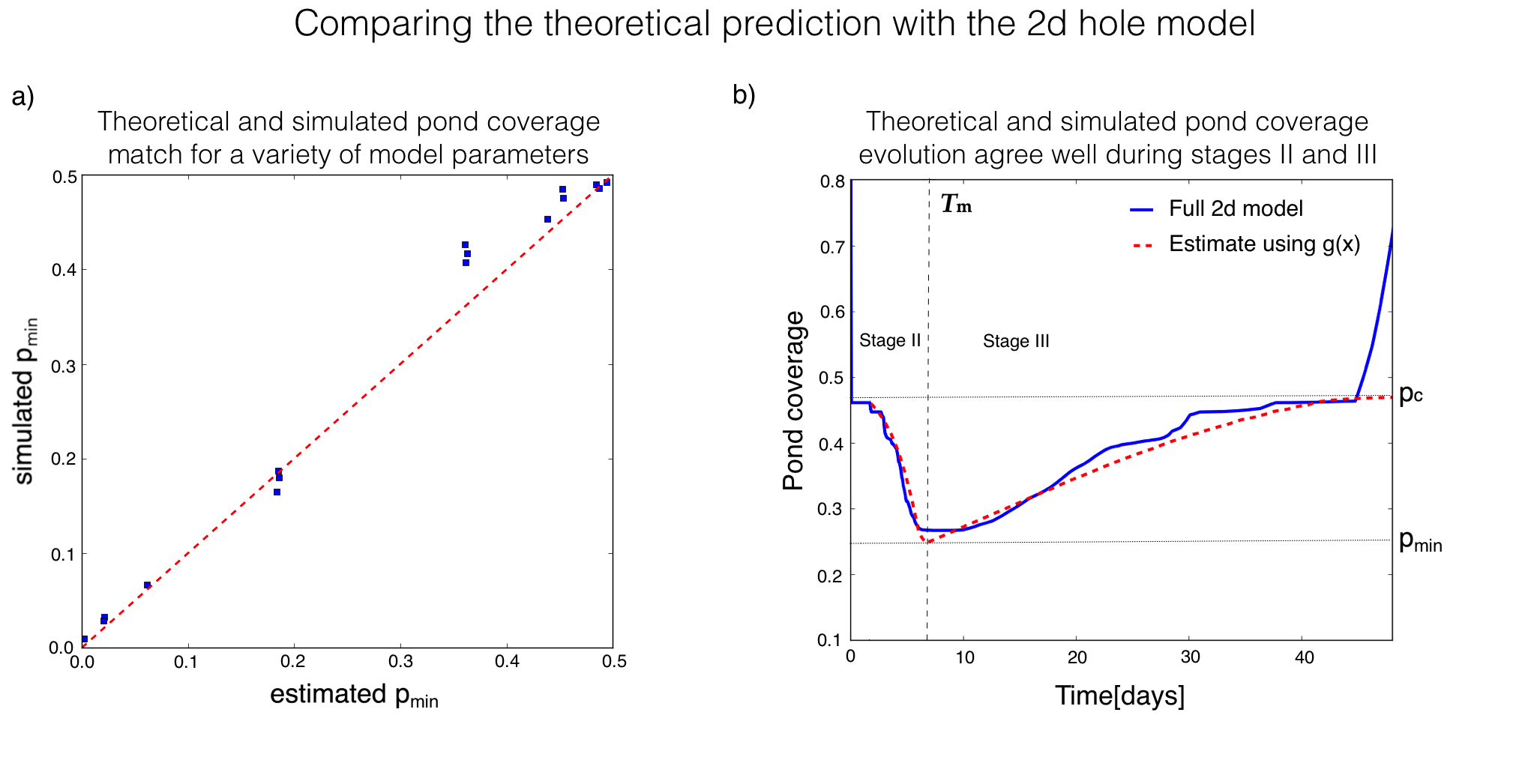
Figure 3: a) Post-drainage pond coverage, $p_{\text{min}}$, found using our full 2d model against the coverage estimated using Eq. 13. Each point is a separate simulation with different rates of ponded ice melt and hole opening timescales. The red dashed line marks the 1:1 ratio. b) Pond coverage evolution using the full 2d model (blue line) and estimated using Eqs. 12 and 14 (red dashed line). Time of memorization, $T_{\text{m}}$, percolation threshold, $p_{c}$, and the post-drainage pond coverage, $p_{\text{min}}$, are marked with dashed and dotted black lines. Times earlier than $T_{\text{m}}$ correspond to stage II of pond evolution, while later times correspond to stage III.

Holes form mainly as enlarged brine channels (Polashenski et al., 2012). Such brine channels are tubes, roughly a centimeter in diameter, that run through the entire thickness of the ice (Cole and Shapiro, 1998). B15Not all brine channels span the entire depth of the ice (Lake and Lewis, 1970), so, likely, only some can become enlarged into holes. Polashenski et al. (2012) showed that, depending on the channel radius, ice temperature, salinity, and other bulk properties, a channel can either close or enlarge when meltwater flows through it. In the beginning all the channels are closed, but as the ice warms, some of them start to open. Polashenski et al. (2017) suggested that as the ice temperature passes through a particular threshold, some channels begin to open, while above a certain temperature nearly all channels become open.

Based on the above, we choose to model the evolution of the number of holes as

$$N(t)=N_{0}F\big{(}\frac{t-t_{0}}{T_{\text{h}}}\big{)}\text{ , }$$ (8)

$$t_{0}\sim-T_{\text{h}}F^{-1}(\frac{1}{N_{0}})\text{ , }$$ (9)

where $N_{0}$ is the total number of brine channels that can possibly become holes, $F$ is the fraction of those channels that become holes by time $t$, and can be seen as a cumulative distribution of some underlying probability density function $f$, and $T_{\text{h}}$ and $t_{0}$ are the width and the center of this distribution. A37The parameter $t_{0}$ can be interpreted as the time between when the first hole opens and when a fraction of holes, $F(0)$, open. Equation 9 then follows by noting that time $t=0$ corresponds to the opening of the first hole, so that $N(t=0)=1$. This relationship is approximate because the timing of opening the first hole is intrinsically stochastic. So, each independent model run will have a slightly different $t_{0}$ even if all large-scale parameters are the same (see SI section LABEL:sec:holedist). Nevertheless Eq. 9 shows that, to first order, $t_{0}$ is not an independent parameter. Currently, we are only assuming that the distribution $F$ has a well-defined width, controlled by a unique hole opening timescale, $T_{\text{h}}$. Thus, we are assuming that a significant fraction of holes open within time $T_{\text{h}}$, and that within several $T_{\text{h}}$ almost all of the brine channels open. From Eq. 8, we can see that under these relatively broad assumptions, ice microphysics contributes to pond evolution by changing the hole timescale, $T_{\text{h}}$, number of channels, $N_{0}$, and the distribution $F$.

The hole opening timescale, $T_{\text{h}}$, depends on specific mechanisms that control the formation of holes and is, therefore, more difficult to relate to measurable parameters than the memorization timescale (Eq. 7). Polashenski et al. (2017) suggested that a significant fraction of holes open up when the ice interior warms by some amount $\Delta\theta\sim 1^{\circ}\text{C}$ beyond the temperature at which the first hole opens. This suggests a way to relate $T_{\text{h}}$ to physical parameters in a way that is consistent with observations, but we note that a better understanding of hole formation physics is needed to make this estimate more realistic. Therefore, we estimate

$$T_{\text{h}}\approx\frac{\Delta\theta}{\text{d}\theta/\text{d}t}\text{ , }$$ (10)

$$\frac{\text{d}\theta}{\text{d}t}\approx\frac{\theta_{0}^{2}}{\rho_{i}\gamma S}\Big{(}c^{*}k\frac{\theta_{0}}{H^{2}}+(1-\alpha_{p})F_{\text{sol}}\kappa e^{-\kappa z^{*}}\Big{)}\text{ ,}$$ (11)

where $\text{d}\theta/\text{d}t$ is the warming rate of the ice interior, $S$ is the ice salinity, $\theta_{0}$ is a reference temperature in degrees Celsius at which the holes tend to start opening, $\gamma$ is a constant that relates the ice heat capacity to the salinity, $k$ is the thermal conductivity of the ice, $\alpha_{p}$ is the albedo of ponded ice, $\kappa$ is the extinction coefficient from Beer’s law, $z^{*}$ is the depth within the ice at which we are estimating the warming rate, and $c^{*}$ is a constant that accounts for the shape of the vertical temperature profile. Equation 11 is an order-of-magnitude estimate of the ice warming rate in terms of measurable parameters that we derive in SI section LABEL:sec:heat following Bitz and Lipscomb (1999). We note, however, that $T_{\text{h}}$ can change by a factor of several by changing the under-constrained properties such as the depth at which the freshwater plugs form or the reference temperature, $\theta_{0}$.

With a model for hole opening, we can estimate the pond evolution, $p(t)$, and pond coverage after drainage, $p_{\text{min}}$, by combining Eqs. 3 and 8

$$p(t)\approx p_{c}g\left(cN_{0}\frac{l_{0}^{2}}{L^{2}}F\left(\frac{t-t_{0}}{T_{\text{h}}}\right)\right)\text{ , } t<T_{\text{m}}$$ (12)

$$p(t)\approx p_{\text{min}}\equiv p(T_{\text{m}})\text{ , } t>T_{\text{m}}\text{ . }$$ (13)

These equations can be solved once we assume a concrete distribution $F$. As a default, we used a cumulative normal distribution $F$ throughout the paper. In SI section LABEL:sec:holedist, we explored other distributions and showed that, due to the fact that $N_{0}$ is very large, pond evolution only depends on the tail of $F$. Since $T_{\text{m}}$ depends on $p_{\text{min}}$ through Eq. 7, Eqs. 7 and 13 have to be solved simultaneously for $p_{\text{min}}$ and $T_{\text{m}}$. To test the above relations, we compared $p_{\text{min}}$ found using Eq. 13 against our full 2d hole model (see SI section LABEL:sec:compare for details). Figure 3a shows that the simulations and the estimates agree well, confirming that the above equations do in fact approximately solve the full hole model. In SI section LABEL:sec:params, we use Eqs. 7 and 9 - 13 to explore how the pond coverage depends on physical parameters.

VI Pond evolution during stage III

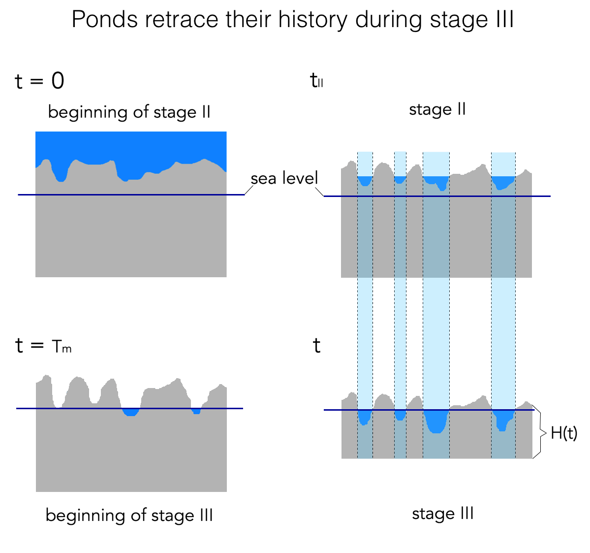
Figure 4: A schematic of pond evolution under the assumptions stated in section VI. Stage II begins at time $t=0$, with a high pond coverage and ice surface above sea level. At a time $t_{\text{II}}$ during stage II, water level decreases and pond coverage evolves according to Eq. 12. We assume that the ponds are approximately level so their boundaries define a level-set of the topography. Ponded ice may melt in a complicated way, but we assume that bare ice melts spatially uniformly, so the topography left in the wake of the decreasing water level remains unchanged. When ponds reach sea level, stage II ends and stage III begins. During stage III, ponds are defined by the intersection of sea level and the ice topography, and are thus also level-sets of the topography. The above-sea-level topography at the beginning of stage III determines pond evolution during stage III if there is no lateral melt of pond walls. As the ice thins, sea level intersects this topography at different levels. Since this topography has not changed since the last time it was ponded during stage II, there exists a time $t$ during stage III for which the horizontal distribution of ponds is the same as it was at a time $t_{\text{II}}$ during stage II. In this sense, ponds retrace their history. For visual clarity, we have not shown ice thinning during stage II, but it is assumed that ice thins throughout its evolution.

We have shown that the universal function $g(\eta)$ can be used to solve our hole model, providing a formula for pond coverage evolution during stage II. In our model so far, we have neglected ice thinning, and so were unable to explicitly model stage III of pond evolution. Here we will extend our analysis to this stage as well. We will show that the same function $g(\eta)$ also governs the evolution of pond coverage during stage III under certain assumptions.

A15B7We start by explaining the relationship between pond behavior during stage II and stage III (see Fig. 4). To this end, we have to make several assumptions. In particular, we will assume that ponds are approximately level during stage II, that bare ice melts at a spatially uniform rate, that pond coverage only decreases during stage II and only increases during stage III, and that there is no lateral melt during stage III. If ponds during stage II are approximately level, ice at the pond boundaries has approximately the same height, and is thus, approximately, a level-set of the ice topography. As the ponds drain and the water level decreases during stage II, ice at the pond boundaries quickly becomes pond-free and, assuming that bare ice melts at a spatially uniform rate, remains approximately level for the remainder of stage II. During stage III, ponds are drained to sea level nearly completely, so pond boundaries are again level-sets of the ice topography and the pond coverage is equal to the fraction of the ice surface below sea level. If there is no lateral melting of pond walls, pond growth during stage III is entirely due to ice thinning and consequent freeboard sinking, which leads to more of the ice surface falling below sea level. Thus, the above-sea-level topography, which consists only of bare ice, does not change until it is submerged. This means that pond coverage at any time during stage III is uniquely determined by the above-sea-level topography at the beginning of stage III, which is unchanged since it was last ponded during stage II, and the current ice thickness, $H(t)$, which determines the freeboard height. Therein lies the connection between stage II and stage III ponds - both are approximately level-sets of the same topography created in the wake of decreasing water level during stage II. In this sense ponds during stage III approximately retrace their history - B8for every water level during stage II there exists a corresponding ice thickness during stage III so that ponds are approximately the same. Using this idea, we can estimate the pond evolution during stage III.

In order for ponds to retrace their history, the assumptions we stated at the beginning of the previous paragraph have to hold. These assumptions are likely satisfied in reality, at least approximately. In our hole model, ponds are certainly not exactly level during stage II, since this would prevent them from becoming disconnected. Nevertheless, this assumption likely holds well enough so that ponds approximately retrace their history, as we show below by directly simulating stages II and III in our model. Note that we only had to assume that bare ice melts spatially uniformly, and made no assumptions about ponded ice - whichever way the ponded ice melts, the topography set during stage II will be re-submerged during stage III, and ponds will retrace their history. However, a spatially non-uniform melt rate of ponded ice may affect the mapping between stage II and stage III ponds, so, to construct this mapping explicitly, below we will consider only the case where ponded ice does melt uniformly in both time and space.

Now, we can proceed to explicitly relate stage II and stage III pond coverage. Consider a time $t_{\text{II}}$ since the beginning of stage II at which the pond coverage is $p_{\text{II}}(t_{\text{II}})$. A15.2B9If the ice is flat compared to freeboard thickness at the beginning of stage II and ponded ice melts uniformly, the depth of topographic depressions created by preferential ponded ice melting by time $t_{\text{II}}$ is approximately $\delta h(t_{\text{II}})\approx\frac{\text{d}h_{\text{diff}}}{\text{d}t}t_{\text{II}}$. Thus, ice that was ponded at $t_{\text{II}}$ will have carved depressions of at least $\delta h$ by the beginning of stage III. On the other hand, since pond coverage only decreases during stage II, any non-ponded location at $t_{\text{II}}$ will have carved depressions less than $\delta h$ deep by the beginning of stage III. During stage III, depressions of depth $\delta h$ will be below sea level when the freeboard height, $h$, is less than $\delta h$. So, if the ponds retrace their history, we can use the relationship $h(t)=\delta h(t_{\text{II}})$, to find the time $t_{\text{II}}$ at which the pond coverage was the same as it is at time $t$ during stage III. Thus, we find $t_{\text{II}}(t)\approx\frac{h(t)}{\text{d}h_{\text{diff}}/\text{d}t}$.

Note that $t_{\text{II}}$ has the same form as the memorization timescale, $T_{\text{m}}$, given by Eq. 7 - both are a ratio of a freeboard thickness, $h$, and a differential melt rate, $\text{d}h_{\text{diff}}/\text{d}t$, the only difference being that Eq. 7 is estimated using $h$ at the end of stage II and $t_{\text{II}}$ is estimated using $h$ at some time, $t$, during stage III. So, we can use $T_{m}(t)$ calculated by Eq. 7 using the values for ice thickness and pond coverage at time $t$, and define $t_{\text{II}}(t)=T_{\text{m}}(t)$. We thus relate stage II and III pond coverage as $p(t)=p_{\text{II}}(T_{\text{m}}(t))$. Therefore, using Eq. 12, the pond evolution during stage III can be approximately captured as

$$p(t)\approx p_{c}g\Big{(}cN_{0}\frac{l_{0}^{2}}{L^{2}}F\Big{(}\frac{T_{\text{m}}(t)-t_{0}}{T_{h}}\Big{)}\Big{)}\text{ , }$$ (14)

$$T_{\text{m}}(t)\approx\frac{h(t)}{\text{d}h_{\text{diff}}/\text{d}t}=\frac{l_{m}}{\Delta\alpha F_{\text{sol}}}\frac{\rho_{w}-\rho_{i}}{\rho_{w}}\frac{H(t)}{1-p(t)}\text{ .}$$ (15)

This equation is applicable after complete pond drainage to sea level. In SI section LABEL:sec:compare, we note that the transition between stage II to stage III can be estimated as the time at which $p(t)$ approximated using Eq. 14 exceeds $p(t)$ estimated using Eq. 12 (i.e., when $t>T_{\text{m}}(t)$). After choosing $F$, Eqs. 12 and 14 together describe the pond evolution after the beginning of pond drainage below the percolation threshold.

We test these equations against our full 2d hole model that includes ice thinning and assumes a constant thinning rate, $\text{d}H/\text{d}t$, in Fig. 3b (see SI section LABEL:sec:compare for more details). We can see that the two agree well most of the time, suggesting that our assumption about ponds retracing their history is justified in our model. Since $g\leq 1$, Eqs. 12 and 14 predict that $p_{c}$ is an upper bound on pond coverage during stages II and III. This is approximately obeyed in the full hole model where the pond coverage during stage II quickly falls below the percolation threshold after the first several holes, and where the ice quickly floods during stage III after pond coverage reaches $p_{c}$. The rapid flooding after the pond coverage reaches $p_{c}$ during stage III in the model is due to the fact that we assumed the ice was very flat at the beginning of stage II. In reality, this assumption may not strictly hold, but we still expect the percolation threshold to be an approximate upper bound after which flooding, and subsequent ice disintegration, follows more rapidly than before.

VII Comparison with observations

We can now proceed to compare our model predictions to observations. We describe the details of these comparisons in SI section LABEL:sec:data. Polashenski et al. (2012) collected extensive field data on pond coverage and ice properties during the summer of 2009 near Barrow Alaska. Using their measurements and Eqs. 7 and 9 - 11, we were able to estimate all of the parameters that enter Eqs. 12 and 14. Figure 5a shows the measured pond coverage, along with our predictions and an estimated margin of error due to uncertainty in the physical parameters that enter the pond evolution equations, while Table 1 summarizes our estimates of the timescales $T_{\text{m}}$ and $T_{\text{h}}$, the minimum pond coverage, $p_{\text{min}}$, and the percolation threshold, $p_{c}$, as well as their margin of error. Since so many physical parameters contribute to pond evolution, even modest uncertainty in measurements leads to relatively large uncertainty in pond coverage. In fact, we find that to match the pond coverage evolution to within 10% all of the physical parameters would have to be known to within about 1%. A33B70Equation 12 predicts that ponds drain instantly to the percolation threshold as soon as the first hole opens. The measurements, on the other hand, show a more gradual decline in pond coverage towards the percolation threshold, likely due to the fact that real holes take time to grow and cannot drain ponds instantly. B17Nevertheless, we can see that observations are consistent with our predictions below the percolation threshold, and our equations capture the pattern of pond coverage variability over time. We can see that within the limited range of reasonable physical parameters, we are able to choose a combination that predicts a pond evolution that accurately matches observations below $p\approx 0.36$.

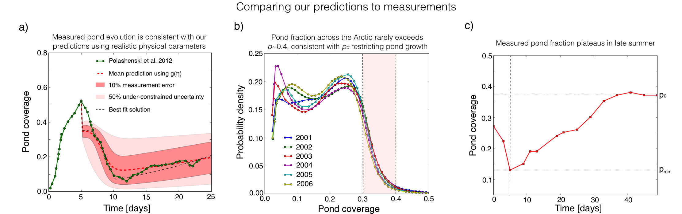
Figure 5: a) The green line represents time evolution of pond coverage measured by Polashenski et al. (2012) near Barrow, Alaska in the summer of 2009. The red dashed line and the dark shaded region are the mean and one-standard-deviation uncertainty of an ensemble of pond coverage evolutions found using Eqs. 12 and 14. For each pond evolution within the ensemble, every physical parameter that enters the pond evolution equations was selected randomly from a normal distribution with a mean estimated using measurements by Polashenski et al. (2012) and a standard deviation equal to 10% of the mean. The black dashed line is the least-squares best fit prediction using parameters that are within the 10% measurement error. The light shaded region is the one-standard-deviation uncertainty region assuming a 10% measurement error for all the parameters directly measured by Polashenski et al. (2012) and a 50% uncertainty for under-constrained microphysical parameters such as the shape parameter for the temperature profile, $c^{*}$, the reference temperature, $\theta_{0}$, and the depth at which the freshwater plugs form, $z^{*}$. Values of 10% and 50% are not estimates of real uncertainties, but were chosen simply to demonstrate the sensitivity to model parameters. We note that the slight increase in the upper boundary of the light shaded region during stage II simply corresponds to increased uncertainty during that time, and no actual pond coverage trajectory increases during stage II. b) Distribution of pond coverage across the Arctic for different years derived from MODIS satellite data (Rösel et al., 2015a). The frequency of observations declines rapidly between $0.3<p<0.4$ and very few observations show $p>0.4$, consistent with our predictions. The light shaded region shows the likely values for the percolation threshold estimated by Popović et al. (2018). c) Observations of pond coverage evolution made along a transect during the 1998 SHEBA mission. The data are taken from Perovich et al. (2003). Horizontal and vertical lines mark the estimated minimum pond coverage, $p_{\text{min}}$, percolation threshold, $p_{c}$, and the timing of the transition between stages II and III.

Table 1: Estimates of the timescales $T_{\text{m}}$ and $T_{\text{h}}$, the minimum pond coverage, $p_{\text{min}}$, and the percolation threshold, $p_{c}$, found using Eqs. 7, 10, 11, and 13. The explored range represents the minimum and maximum estimate of these parameters over an ensemble of pond coverage evolutions corresponding to the dark shaded region in Fig. 5a, while the best fit estimates correspond to the least-squares best-fit pond evolution curve over this ensemble shown as the black dashed line in Fig. 5a.

	$T_{\text{m}}$ [days]	$T_{\text{h}}$ [days]	$p_{\text{min}}$	$p_{c}$
Best fit	4.4	2.0	0.1	0.36
Explored range	(2.3, 9.2)	(1.0,6.6)	(0.0,0.3)	(0.2,0.5)

B11.3As we discussed before, our model predicts an approximate upper bound on pond coverage during stages II and III. In particular, we showed that after the beginning of stage II, ponds quickly drain to $p_{c}$, while at the end of stage III, the entire floe quickly floods when pond coverage exceeds $p_{c}$. This means that ponds likely spend little time at coverage higher than the percolation threshold. Moreover, this approximate upper bound may also be present during stage I. If during stage I there exist large flaws in the ice such as cracks, holes, or even the floe edge, that can quickly drain large volumes of water, the percolation threshold would also represent an upper limit on pond coverage during this stage. If such flaws exist, the pond coverage would in fact be bounded throughout the entire melt season. In Fig. 5b, we show the pond coverage distribution across the entire Arctic estimated from MODIS (Moderate Resolution Imaging Spectroradiometer) satellite data (Rösel et al., 2015a). The frequency of pond coverage observations is relatively high for $p<0.3$ and declines rapidly for higher pond coverage values. Moreover, the pond coverage very rarely exceeds 0.4, consistent with our prediction that an upper bound on pond coverage exists. Values between 0.3 and 0.4 are also consistent with Popović et al. (2018) who estimated $p_{c}$ directly from pond photographs, and found it to be roughly between 0.3 and 0.4. A19B11.2We note that these values for the percolation threshold are about 0.1 lower than $p_{c}$ predicted by the “snow dune” topography, developed in Popović et al. (2020) (and described in SI section LABEL:sec:topos), that accurately matches the pre-melt ice topography and predicts a $p_{c}$ between 0.4 and 0.5. This decrease could be due to processes such as the formation of connecting channels between ponds during pond drainage that change the topography and increase the efficiency of drainage.

B11In the previous section and in Fig. 3b, we showed that our model predicts that the pond coverage will approach $p_{c}$ in the late stages of pond evolution, after which the ice rapidly floods, presumably leading to disintegration. This late-season approach to $p_{c}$ and subsequent rapid flooding may in fact account for the observations by Popović et al. (2018) that late summer ponds are organized close to the percolation threshold. A18Furthermore, observations made during the 1998 SHEBA mission, reported in Perovich et al. (2003), and shown in Fig. 5c, showed stage III pond evolution that strongly resembles our model prediction that pond growth slows down as it approaches $p_{c}$. There, starting from a minimum, the pond coverage increased over a period of roughly 40 days approaching a point ($p\approx 0.37$) after which it approximately stopped changing for the remainder of the field experiment (compare Figs. 3b and 5c). Again, this value of $p\approx 0.37$ is a plausible percolation threshold according to Popović et al. (2018) and our previous discussion in this section.

VIII Discussion

We now discuss how pond coverage in our model depends on physical parameters, how our model might be incorporated into a large-scale sea ice scheme, and the challenges of pond modeling. In the previous sections, we have related the pond evolution to parameters $p_{c}$, $H$, $\alpha_{i}$, $\alpha_{p}$, $F_{\text{sol}}$, $S$, $\Delta\theta$, $\theta_{0}$, $z^{*}$, $N_{0}$, $L$, and $l_{0}$, all of which can be estimated by measurements, at least in principle. However, not all of these parameters are easily estimated in a large-scale model and the qualitative dependence on some of them may not be appropriately captured in our parameterization due to the fact that we do not yet understand hole formation physics well enough.

The timescale $T_{\text{m}}$ depends only on parameters that are available in large-scale models ($H$, $\Delta\alpha$, and $F_{\text{sol}}$). On the other hand, the hole opening timescale, $T_{\text{h}}$, depends on hole formation physics and is, thus, much more difficult to estimate. In our parameterization, $T_{\text{h}}$ is both a function of parameters available in large-scale models ($H$, $S$, $\alpha_{p}$, and $F_{\text{sol}}$) and those that can only be loosely constrained by field observations ($\Delta\theta$, $\theta_{0}$, and $z^{*}$). In addition to this, $T_{\text{h}}$ in our parameterization depends on salinity, $S$, and reference temperature, $\theta_{0}$, in a qualitatively counter-intuitive way (see SI section LABEL:sec:params). Namely, in our parameterization of $T_{\text{h}}$, we directly related the fraction of open holes to the ice interior temperature following the suggestion of Polashenski et al. (2017). This led to $T_{\text{h}}$ being higher at higher $S$ and $\theta_{0}$, since these conditions imply a lower ice warming rate. This is counter-intuitive because higher salinity and reference temperature also imply a higher brine volume fraction which, in reality, likely increases the hole formation rate, lowering $T_{\text{h}}$. For this reason, we believe that the assumption of using the ice temperature to diagnose hole opening may need to be reconsidered. B44Another parameter such as, for example, ice porosity, may be better suited to diagnose when holes in the ice begin to form.

The dependence of pond coverage on most of the physical parameters in our model is qualitatively robust. An exception to this is the ice thickness. We find that the effect of thickness, $H$, depends qualitatively on the details of hole formation physics. Increasing $H$ has two effects - 1) it raises the freeboard, increasing $T_{\text{m}}$, and 2) it slows down the warming of the ice interior, increasing $T_{\text{h}}$. Therefore, the way in which $H$ affects pond coverage qualitatively depends on whether the effect on $T_{\text{m}}$ or $T_{\text{h}}$ dominates. A4.2 In SI section LABEL:sec:params, we show how a minor change in the assumptions about the hole formation physics may completely change the effect of ice thickness. We note that Skyllingstad et al. (2015), who ran pond-resolving simulations that include pond drainage, did not find a systematic relationship between pond fraction and the initial ice thickness, consistent with our discussion here. Establishing the correct relationship between ice thickness and pond coverage may be important for estimating the strength of the ice-albedo feedback under global warming. To that end, our model could be used to test hypotheses about hole formation physics by making predictions about the relationship between pond coverage and physical parameters that can be tested against field data that exploit the natural variability in environmental conditions across the Arctic.

We believe that the dependence of pond coverage on all other physical parameters predicted by our model is qualitatively correct, even if it may be somewhat quantitatively inaccurate because of poor understanding of hole formation physics. In Fig. LABEL:fig:params of SI section LABEL:sec:params, we specifically look at the minimum pond coverage, $p_{\text{min}}$. There, we show that $p_{\text{min}}$ increases with the domain size, $L$, percolation threshold, $p_{c}$, ice albedo, $\alpha_{i}$, temperature range for hole opening, $\Delta\theta$, and the depth at which ice plugs tend to form, $z^{*}$. We show that it decreases with typical pond size, $l_{0}$, and pond albedo, $\alpha_{p}$. Finally, we show that it only weakly depends on the solar flux $F_{\text{sol}}$ and brine channel density, $n_{0}$. We note that prior to this investigation, it was not recognized that geometric parameters $L$, $l_{0}$, and $p_{c}$ can have any effect on pond coverage.

A34In addition to the uncertainties we discussed above, our model predicts that accurately estimating pond coverage evolution is a fundamentally difficult problem, regardless of how well we understand the ice and pond physics. Namely, our model predicts that pond coverage is highly sensitive to physical parameters, so even small errors in measurements or natural variability can lead to large variations in predicted pond coverage. In particular, as we have noted in the previous section, to be able to predict pond coverage to within several percent in our model, all of the physical parameters need to be known to within about 1%. A37.2Moreover, even if all of the bulk parameters are perfectly known, we still cannot perfectly constrain the pond evolution. Since the timing of the opening of the first drainage hole is intrinsically stochastic (see Eq. 9 and SI section LABEL:sec:holedist), pond coverage will fluctuate from one situation to another even if all of the bulk parameters are identical. In our simulations this stochasticity in the timing of the first hole contributed to about $5\%$ variability in minimum pond coverage, $p_{\text{min}}$.

Ice albedo is a critical parameter in large-scale models that controls the thermal evolution of the sea ice cover. Since melt pond coverage is a primary control on albedo, Eqs. 12 and 14 can be straightforwardly used as a physically sound and computationally inexpensive parameterization of the albedo evolution during stages II and III of pond evolution. In addition, these equations can be supplemented with a similarly inexpensive equation for stage I developed in Popović et al. (2020). However, our discussion above clearly highlights two issues relevant for employing our model in a large-scale scheme - 1) ice microphysics that governs hole formation needs to be better understood, and 2) pond coverage possesses a built-in sensitivity to environmental conditions and stochasticity that greatly amplify any uncertainty that may exist in measurements. We emphasize that these challenges are not an artifact of our hole model - any model of melt ponds will need to address hole formation physics to accurately capture the dependence on physical parameters, and any model will likely face a similar sensitivity to physical parameters which simply stems from the fact that there are many parameters that control pond evolution. Our work here reveals that the natural way to parameterize pond coverage is through the number of drainage holes per characteristic area of the surface, $\eta$. Thus, if any model were able to track $\eta$ directly rather than break it down into a multitude of environmental parameters, uncertainty in estimates of pond coverage would greatly reduce. If such a reduction is not feasible, the low computational cost of our model could be exploited to assign a distribution of pond coverage at each grid point of a large-scale model rather than to provide a single pond evolution trajectory. In addition to the issues above that are likely a generic feature of melt pond physics, some of the simplifying assumptions are specific to our model, such as, for example, neglecting the formation of connecting channels between ponds or assuming that drainage through holes is instantaneous. These assumptions may also need to be further examined to make sure our model can be used as a reliable albedo parameterization.

IX Conclusions

Our paper revolves around the observation that the percolation threshold is of special significance for melt ponds. We showed that this stems from the fact that ponds typically drain through large holes, making drainage easy above the threshold and difficult below. In this way the percolation threshold represents an approximate upper bound on pond coverage throughout most of, or, in some cases, the entire summer. The fact that pond coverage often lingers around the percolation threshold leads to universality that greatly simplifies this otherwise complex problem, and allows us to write a simple formula that describes pond evolution throughout most of the melt season. It also makes it possible to connect pond evolution with measurable parameters. Observations are consistent with all of our predictions. The formula for pond coverage we provided requires very little computational power. Therefore, it holds promise as a physical, accurate, and computationally inexpensive parameterization of pond coverage in large scale models. Finally, our work connects melt ponds with the broader field of critical phenomena and our results regarding the universality of drainage may be applicable to other systems whose evolution is governed by a critical point of a phase transition.

Table 2: A table of parameters used in the paper, their default values, and plausible ranges where it was possible to estimate the ranges.

	Name	Unit	Default value	Plausible range	Source
$t$	Time	day		(0,30)
$p$	Pond coverage	None		(0,1)
$p_{c}$	Percolation threshold	None	0.35	(0.3,0.5)	(Isichenko, 1992; Popović et al., 2018), this work
$p_{\text{min}}$	Minimum pond coverage	None		(0,$p_{c}$)
$\Pi$	Renormalized pond coverage	None		(0,1)
$l_{0}$	Typical pond length-scale	m	5.5	(5.2,5.8)	(Popović et al., 2020)
$L$	Drainage basin size	km	1.5		(Polashenski et al., 2012)
$n_{0}$	Density of brine channels	$\text{m}^{-2}$	100	(60,120)	(Golden, 2001)
$N_{0}$	Number of brine channels	None	$2.25\times 10^{8}$		Inferred from $n_{0}$ and $L$
$N$	Number of open holes	None		(1,$N_{0}$)
$\eta$	Renormalized number of open holes	None			this work
$c$	Numerical drainage constant	None	3	(3,4.1)	this work
$\rho_{i}$	Density of ice	$\text{kg m}^{-3}$	900
$\rho_{w}$	Density of water	$\text{kg m}^{-3}$	1000
$l_{m}$	Latent heat of melting	$\text{kJ kg}^{-1}$	$334$
$\gamma$	Constant relating heat capacity to salinity	$\text{kJ kg}^{-1}\text{ppt}^{-1\circ}\text{C}$	18		(Ono, 1967; Bitz and Lipscomb, 1999)
$k$	Thermal conductivity	$\text{W m}^{-1\circ}\text{C}^{-1}$	1.8	(1.3,2.0)	(Untersteiner, 1964; Bitz and Lipscomb, 1999)
$\kappa$	Extinction coefficient	$\text{m}^{-1}$	1.5		(Untersteiner, 1961; Bitz and Lipscomb, 1999)
$H$	Ice thickness	m	1.2	(0.5,3)
$h$	Post-drainage freeboard thickness	m	0.1	(0.05,0.3)
$F_{\text{sol}}$	Time-averaged solar flux	$\text{W m}^{-2}$	254	(140,350)	(Polashenski et al., 2012)
$\Delta\alpha$	Albedo difference between pond and ice	None	0.4	(0.3,0.5)	(Polashenski et al., 2012; Perovich, 1996)
$\alpha_{p}$	Pond albedo	None	0.25	(0.2,0.3)	(Perovich, 1996)
$S$	Ice salinity	ppt	3		(Polashenski et al., 2012)
$\theta_{0}$	Reference ice interior temperature	∘C	-1.2		(Polashenski et al., 2017)
$\Delta\theta$	Temperature range for hole opening	∘C	0.7		(Polashenski et al., 2017)
$c^{*}$	Temperature profile effect on heat diffusion	None	2	(1,10)	this work
$z^{*}$	Depth at which ice plugs form	m	0.6		(Polashenski et al., 2017)
$t_{0}$	Center of the hole opening distribution	day	13.4		this work
$T_{\text{m}}$	Memorization timescale	day	4.4		this work
$T_{\text{h}}$	Hole opening timescale	day	2.0		this work