DeltaCNN: End-to-End CNN Inference of Sparse Frame Differences in Videos

Abstract

Convolutional neural network inference on video data requires powerful hardware for real-time processing. Given the inherent coherence across consecutive frames, large parts of a video typically change little. By skipping identical image regions and truncating insignificant pixel updates, computational redundancy can in theory be reduced significantly. However, these theoretical savings have been difficult to translate into practice, as sparse updates hamper computational consistency and memory access coherence; which are key for efficiency on real hardware. With DeltaCNN, we present a sparse convolutional neural network framework that enables sparse frame-by-frame updates to accelerate video inference in practice. We provide sparse implementations for all typical CNN layers and propagate sparse feature updates end-to-end – without accumulating errors over time. DeltaCNN is applicable to all convolutional neural networks without retraining. To the best of our knowledge, we are the first to significantly outperform the dense reference, cuDNN, in practical settings, achieving speedups of up to 7x with only marginal differences in accuracy. Our CUDA kernels and PyTorch extensions can be found at https://github.com/facebookresearch/DeltaCNN.

1 Introduction

Convolutional neural networks (CNN) are the state-of-the-art method for many image understanding tasks such as object detection, segmentation and pose estimation. Compared to multi-layer perceptrons, they require fewer parameters by spatially sharing parameters and perform better on image understanding tasks. However, to address the increasing complexity of datasets and tasks, CNNs have grown to hundreds of convolutional layers requiring tens of billions of floating point operations (FLOPs).

In the last few years, researchers have found many ways to lower the cost of convolutional layers: Depth-wise separable convolutions [28], optimizing the ratio between pixels, channels and layer count [30], quantization [22, 14, 20], pruning [13, 18] and specialized hardware [12, 6, 5], to name a few. While these methods achieve a significant improvement in general purpose inference, there still is strong interest to further reduce the computational cost of CNNs, particularly for real-time applications on mobile devices.

Recently, researchers started to exploit the temporal similarity commonly seen in surveillance cameras, license plate recognition cameras or webcams [33, 9, 23, 16, 19, 34, 24, 3, 27, 11, 1]. These applications often use CNNs on video input from fixed cameras, where high frame-to-frame similarity offers an orthogonal direction to reduce computational complexity. State-of-the art frameworks for CNNs process each frame individually and therefore are not able to exploit frame-to-frame similarity. By reusing the results from previous frames in unchanged regions, the computational cost can theoretically be reduced greatly [24, 3, 11, 1] without reduction in accuracy. Furthermore, small and insignificant updates can be truncated to retain a high level of sparsity in activation throughout all layers of the CNN with only marginal differences in the final output [24, 11].

While researchers have shown that truncating small changes increases the sparsity and thereby reduces FLOPs theoretically, leveraging data sparsity efficiently to speed up inference with actual hardware remains an unsolved challenge. Since parallel SIMD devices, like GPUs, are typically used for CNN inference due to the advantage in operations per watt and memory bandwidth, it is necessary to evaluate the real-word speedup of sparse neural networks on such devices. Specialized inference hardware as well as GPUs are less efficient for excessive conditional statements than CPUs and suffer under less structured memory access, both conditions that naturally arise when processing sparse activations in neural networks. Thus, previous research results on sparse activation in CNNs do not translate to high speedup numbers in practice.

In this paper, we present the first fully sparse CNN, DeltaCNN, working on and optimized for GPUs. Our implementation translates potential savings of sparse activation into real speedups in practice, outperforming the state-of-the-art cuDNN dense inference by a factor of up to 7x. The main contributions of this paper are:

• We propose DeltaCNN, the first sparse CNN with sparse data access end-to-end, from the input to the output for all layers, including convolution, pooling, activations, upsampling, normalization, etc. DeltaCNN is applicable to all CNNs with minor adaptation without retraining.

• We tackle memory bandwidth and control flow issues of sparse neural networks by a new kernel design involving masks and caches. We open source, to the best of our knowledge, the first GPU implementation of CNN operators for sparse input and output.

• We show the first GPU-based demonstration of leveraging data sparsity for CNN acceleration by speeding up three networks for object detection and human pose estimation on three types of GPUs by up to 7x.

Our evaluations on three GPU architectures show that DeltaCNN is efficiently implemented, matching the speed of cuDNN when operating without sparsity. In sparse mode, we achieve speedups of up to 7x over cuDNN.

2 Related Work

Recent work on exploiting frame-to-frame similarity in videos can coarsely be divided in two groups: optimized model architectures and exploiting feature sparsity by truncating insignificant updates.

2.1 Efficient video CNN architectures

Efficient CNNs aim to reduce the frequency in which the most expensive part of the network, the backbone, is processed. Two path models use a fine-grained feature generation on key frames and a coarse-grained update path for frames in between [9, 23]. Alternatively, the fine-grained features can be adapted directly, e.g. by using optical flow of the network input [16, 34]. Our approach does not require any changes to the network architecture and automatically performs fine-grained updates where required.

2.2 Sparsity in videos

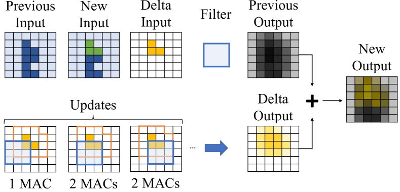
Figure 1: Working principle of spatially sparse convolutions for videos. Computing the difference between the current and previous input, large parts of convolution input become zero (white). Since zero valued inputs do not contribute to the output, these values can be skipped to reduce the number of operations.

Data sparsity in CNNs can be understood as zero-valued features in the feature maps. While activation functions like ReLU already lead to some level of feature sparsity, sparsity in videos can typically be increased greatly by using the difference between the current and the previous frame as input (see Figure 1). This way, background and static features become zero and can be skipped. This characteristic is utilized both in 2D [24, 3, 11, 1] and in 3D [25] CNNs.

Update truncation Recurrent Residual Module (RRM) [24] and CBinfer [3] show that sparsity can be increased even further by truncating insignificant updates without significant loss of accuracy. Contrary to them, Skip-Convolution [11] does not truncate input features, but output features instead. This can lead to higher sparsity, but requires dense updates at a regular schedule (4-8 frames). We use a combination of these ideas. Like Skip-Convolution and CBInfer, we use a spatial (per pixel) sparsity, since structured sparsity better suits SIMD architectures than per value sparsity. Like RRM, we decide per input pixel if an update is required. While having a single input pixel triggering an update of many output pixels may increase FLOPs compared to Skip-Convolution, it is crucial in enabling a continuous inference in sparse mode without accumulating errors over time.

Caching the previous state RRM, CBInfer and Skip-Convolution cache input and output feature maps from previous frames at every convolutional layer to process the differences, increase sparsity and then accumulate the outputs together with dense outputs from previous frames. All operations between convolutions are processed densely. While this strategy reduces FLOPs, it increases memory transfer. To reduce the memory overhead, [1] proposed to only store input and output buffers on key convolutional layers and only use frame differences in between. This approach fails for non-linear layers like pooling or activation functions and may lead to significant errors (see Section 3.1). DeltaCNN performs all operations sparsely, by comparing only the input features (camera image) against the complete previous input, propagating the sparse feature updates throughout all layers. The dense results are only accumulated at the final layer. This way, we also accelerate non-convolutional layers like pooling, upsampling and activations. Furthermore, we avoid switching between sparse and dense computations and only need to cache accumulated values for nonlinear layers, reducing the number of caches compared to [24, 3, 11], without loss in accuracy.

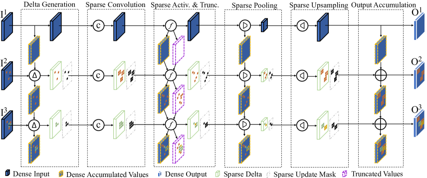
Figure 2: Illustration of inference over three frames using DeltaCNN for a toy network that consists of convolution, activation, pooling, and upsampling layers. The first frame $I^{1}$ is processed densely and is used to initialize the buffers for Dense Accumulated Values. In subsequent frames, Delta Generation subtracts the previous input from the current to generate an Update Mask and a Sparse Delta feature map containing only significant pixel updates. After Sparse Convolution, causing the update mask to dilate, Sparse Activation & Truncation truncates small values to increase sparsity. After the final layer, the Sparse Delta output is accumulated onto the previous output buffer to generate a Dense Output $O^{i}$ for frame $I^{i}$.

2.3 CNN kernels for sparse data

While RRM and Skip-Convolution showed that sparsity in videos can be used to significantly lower FLOPs, they could not show that their approach translates to wall-clock time improvements compared to state-of-the-art dense CNN frameworks. Existing sparse convolution implementations like Sparse Blocks Network (SBNet) [26] and Submanifold Sparse Convolutional Network (SSC) [10] utilize data sparsity to accelerate inference, but are not designed for video inference. Both of these methods assume that the input data is inherently sparse, like handwriting or object boundaries in 3D volumes for SSC, or semantic segmentation masks for SBNet. They do not utilize any mechanism like a cache for storing the dense state of previous frames, and can therefore not be applied on videos. Pack and detect [17] performs full convolutions only on key frames and continuous updates on a smaller image containing the previously detected regions of interest. Unfortunately, the packing operations lead to a large overhead to every convolutional layer. CBInfer implements general sparse convolutions and pooling operations optimized for video input. They perform change detection, change indexing, feature gathering, convolution and feature scattering operations for each convolution. This allows them to utilize fine grained sparsity, but comes with significant data movement overhead and requires convolution algorithms which are inferior compared to leading implementations like cuDNN. In contrast, our approach performs the convolution directly on the feature maps without the need for pre- or post-processing. Together with sparse feature maps, we propagate update masks between layers – starting computations only where necessary.

3 Method

We propose DeltaCNN, an end-to-end sparse CNN framework for accelerating video inference by exploiting frame-to-frame similarity. DeltaCNN replaces all dense tensor operations with sparse operations using an update mask to track which pixels to process. DeltaCNN increases the sparsity with minimal changes in the network output, and processes only the sparse frame updates for each layer.

3.1 Delta value propagation

The core feature of DeltaCNN is to propagate sparse frame updates through the network end-to-end (see Figure 2). To reuse computation of previous frames by adding update tensors, we need to support both linear (e.g. convolutions) and nonlinear (e.g. activations) layers in a CNN.

Linearity of convolutions Convolutions ($c$) are linear operators (see Figure 1), i.e.

$$c(x+\delta x)=c(x)+c(\delta x).$$ (1)

This allows us to use the difference between two images, called delta, as input to the convolution. Delta outputs can be fed as input to consecutive convolutions without the need to accumulate delta updates over multiple frames.

Nonlinear layers Most activation functions, however, are nonlinear. For example, the ReLU activation is defined as:

$$f_{ReLU}(x)=max(x,0).$$ (2)

The nonlinearity of the activation function poses a challenge to update previous results by delta updates. For example,

$$f_{ReLU}(-1)+f_{ReLU}(2)\neq f_{ReLU}(1).$$

To solve this challenge, we keep track of accumulated inputs to nonlinear layers.

For a given activation or pooling function $f$, the delta output $\delta y$ is defined as

$$\delta y=f(x+\delta x)-f(x)$$ (3)

with $\delta x$ being the delta input. The difference, $\delta y$, is then used as delta input for subsequent layers. Every nonlinear layer stores its own buffer holding the previous accumulated inputs. The buffers are initialized during the first frame performing dense inference, and kept up-to-date using the delta of the following frames. Previously accumulated inputs implicitly include all biases applied before them. Thus, biases in convolutional and batch normalization layer are only applied in the first frame.

Truncating small updates Since activation functions follow most convolutional layers, and need to operate on every pixel in the feature map, combining activation and truncation into a single operation helps to minimize overhead. The decision about which values can be truncated is made on a per-pixel level; we truncate a given pixel (setting all channels to 0) and mark it unchanged if $\max_{k}|\delta y_{k}|<\epsilon$. If any $|\delta y_{k}|$ is larger than $\epsilon$, the pixel is marked as updated, and we use an accumulated values buffer $x^{A}$ to store the current value at frame $i$,

$$x^{A}_{i}=x^{A}_{i-1}+\delta x.$$ (4)

However, small truncations can add up over time and lead to a decrease in accuracy with every frame. E.g., when the sun is slowly rising, lighting up an outdoor scene, the frame to frame differences are too small to trigger an update, and the accumulated errors cannot be corrected after being dropped once. To solve this issue, we introduce a second buffer $x^{T}$ containing the accumulated truncations since the last update. The truncated values $x^{T}$ are used together with the delta values $\delta x$ and the accumulated values $x^{A}$ in activation functions:

$$\delta y=f(x^{A}+x^{T}+\delta x)-f(x^{A}).$$ (5)

When a pixel is truncated, $\delta x$ is added onto the truncated values buffer $x^{T}$. When a pixel is marked as updated, $x^{A}$ is updated using

$$x^{A}_{i}=x^{A}_{i-1}+x^{T}_{i-1}+\delta x$$ (6)

and the truncated values buffer $x^{T}_{i}$ is set to zero (see Figure 3). Using this technique, DeltaCNN only requires one dense initial frame, and can apply sparse updates indefinitely without accumulating errors over time.

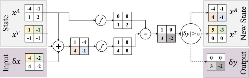
Figure 3: Illustration of the activation and truncation function. It performs activations with accumulated values, truncates the delta $\delta x$ output, and updates the accumulated $x^{A}$ and truncated $x^{T}$ values buffers. In this example, ReLU is used as activation function $f$ and the truncation threshold $\epsilon$ is set to $1.5$. Colored tiles indicate relations between inputs, updated state and output values.

3.2 Design considerations for GPUs

General purpose GPUs allow for the execution of arbitrary code on many core devices. Yet, theoretical instruction reductions often do not translate into efficient GPU code. Non-consistent execution paths and incoherent memory access may lead to significant slowdowns. The key to high convolution performance on GPUs is to optimize memory accesses and generate locally coherent control flow.

Update mask While the changes propagated through the network are sparse, we store the delta features as dense tensors of the same shape in our GPU implementation; with zeroes for locations that can be ignored. To take a previous layer’s sparse output as input, every layer needs to know which pixels were updated. One approach to do this would be a zero-check on all values of the delta input at the beginning of each layer as done by previous work [11, 24, 3].

To avoid loading and checking entire inputs for updates, we propagate – together with the delta feature map – a spatial update mask which contains one value per pixel, indicating if it was updated or not. For every layer, before loading any other data, we first check the update mask of all input pixels and for an entire tile (see below) decide whether to skip all memory operations and computations. Independent of whether a tile is skipped, we write the update mask for the subsequent layer. Using the update mask, we do not need to initialize unprocessed values in feature maps to zero, as they are never read, reducing memory bandwidth even further.

Memory considerations and tiled convolutions Convolutional layers typically make up the majority of processing time in a CNN. While we provide optimized implementations for various layer types, we focus our design discussions around convolutions. These considerations naturally translate to other layer types.

A common approach to optimize memory reuse and locality in 2D convolutions is to process the image in tiles, with each tile processed by a cooperative thread array (CTA). This way, input features and filter parameters can be kept local and reused multiple times. The tile size is chosen in a way to balance the trade-off between memory access and the level of parallelism. Larger tiles reduce memory access but require more resources.

Previous work on sparse convolutions focused on FLOP reductions, but hardly showed wall-clock time improvements in practice. Utilizing sparsity on a fine grained level to avoid unnecessary multiplications requires many additional conditional jumps and may lead to scattered memory operations, easily costing more time than they save, even when the majority of FLOPs can be skipped.

Per-tile sparsity vs. sub-tile sparsity Instead of fine-granular conditions, we employ sparsity on a tile level. In the case of even only one pixel of a tile being updated, the cost is nearly as high as when all pixels are updated, since all filter parameters need to be loaded and multiple output pixels need to be processed and written. For example, consider a tile size of 5x5 output pixels, a 3x3 convolution kernel with 256 channels, requiring a 7x7 input. In this example, one CTA loads 12,544 input features and 589,824 filter parameters and performs 14,745,600 multiplications per tile. If any of the inputs are non-zero, most of the memory transfers are still required; only the number of multiplications could potentially be reduced.

Control flow simplification Convolution operations involve inputs, kernels, and outputs; knowing the association of the three components and their memory location in registers at compile time makes the computation more efficient. Excessive conditional control flows deciding whether to skip a pixel at a sub-tile level require loading variables, performing comparisons, and conditional jumps. This increases the number of executed instructions many times, deteriorating performance.

To avoid fine granular conditional jumps, we propose a hybrid kernel, deciding between three processing modes: skip, dense and very sparse. Tiles with no active input pixels skip all loads and computations. Tiles with five or more active input pixels (out of up to 64) are processed densely without any conditional jumps. Tiles with one to four updated input pixels use a special, highly optimized kernel: it iterates only over a short array of updated pixels gathered from the update mask, removing the need to check the update mask of all pixels many times during multiplication. Furthermore, in this mode we only load filter weights that are required for processing a specific tile. This way, we can reduce memory transactions by up to 8x, e.g. when there is only a single update in the top left corner and it will only affect the top left output pixel. The advantages and disadvantages of sub-tile sparsity are further evaluated in the supplemental material.

3.3 Truncation of insignificant updates

Convolutions dilate the update mask with every layer. A single pixel update in the input quickly expands to 49 pixels after three 3x3 convolutional layers. As not all updates contribute equally to the output of the network, we truncate insignificant updates to increase sparsity and thereby speedup inference. DeltaCNN compares the maximum norm of a pixel with the threshold $\epsilon$ to determine if the pixel update can be truncated.

Typically, the ideal $\epsilon$ will vary between networks and even layers. We auto tune each layer’s $\epsilon$ in a front-to-back manner on a small subset of the training set. Starting with a low $\epsilon$, we iteratively increase the layer’s $\epsilon$ as long as the loss stays below a predefined margin of error, i.e., we allow each truncation layer to contribute equally to the output error. Once the highest threshold below this margin is found, we freeze that layer’s $\epsilon$ and continue with the next in order of execution. Experiments show that we also need to limit the increase in accuracy when tuning for thresholds to avoid overfitting on the small subset of the training set.

3.4 Implementation

With the goal of not only accelerating convolutions, but the entire network, performing as many operations sparsely as possible is crucial. Hence, DeltaCNN provides sparse implementations for most common layers in today’s CNNs: convolutions, batch normalizations, pooling layers, upsampling layers, activations, concatenations and additions. We provide CUDA kernels (as cuDNN replacement) and PyTorch extensions that can be used as a direct replacement for the corresponding PyTorch layers, reusing the original parameters and model logic.

4 Evaluation

We evaluate DeltaCNN on two common image understanding tasks: human pose estimation (Human3.6M[15]) and object detection (MOT16[7] and WildTrack[4]). In both cases, we trained CNNs on video datasets using pre-trained weights from image datasets. After training, convolutional layers and batch normalization layers were fused where possible to improve performance both for the baselines as well as for DeltaCNN. Only the first and last layer for DeltaCNN operate on dense data, converting the dense video input to sparse delta features and converting from delta to dense accumulated outputs, respectively.

In all cases, we use multiple randomly selected training sequences, each consisting of 100 frames, and average the loss over all frames using auto-tuned $\epsilon$ thresholds (as described in Section 3.3). The maximum loss increase over all layers in total is set to 3%, with each layer only allowed to increase the loss by a fraction of this value. For the first truncation threshold, i.e., the input video normalized on ImageNet [8] color range, we use an increased threshold to suppress the background noise, but make sure to stay sensitive enough to capture important motion (0.3 for Human3.6M, 0.5 for MOT16 and WildTrack). The resulting mask is then dilated by 7 pixels to also include smaller updates in the neighboring regions. The effect of using large thresholds together with dilation on the input image compared to small thresholds without dilation is evaluated in Figure 4.

Input

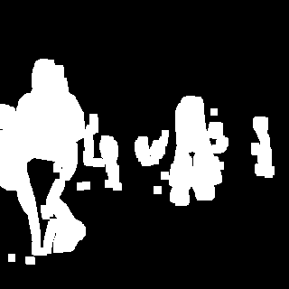
(a) Mask w/ dilation

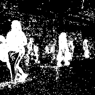
(b) Mask w/o dilation

Figure 4: Input masks generated using a threshold of $\epsilon=0.5$ and 7 pixel dilation (a) and using a threshold of $\epsilon=0.15$ without dilation (b). The dilated version runs 8% faster and achieves slightly more accurate results on the MOT16 dataset.

4.1 Human pose estimation

For human pose estimation, we use two different CNN architectures: HRNet [29] and Pose-ResNet [32]. The networks are initialized with weights pre-trained on ImageNet [8] and further trained on Human3.6M [15] with an input resolution of $384$x$384$. Human3.6M is designed as a benchmark and does not provide the ground truth poses for the test set publicly. As our evaluation includes frame-by-frame analysis of accuracy, FLOPs and speedup, we use parts of the training set (Subject S11) for testing, and exclude them during training. The test set contains 120 videos with an average length of 1927 frames and therefore serves as a reference for how much error accumulates over long time evaluations with DeltaCNN.

4.2 Object detection

For object detection, we use EfficientDet [31], based on the parameter- and FLOPs-efficient EfficientNet architecture [30]. The network is trained on two different datasets: Multiple Object Tracking 16 (MOT16) [7] and WildTrack [4]. In both cases, we trained multiple configurations of EfficientDet on the video datasets with a 80/20 train/test split and initialized the network with weights pre-trained on the COCO dataset [21]. WildTrack provides videos with a frame rate of 60 frames per second (FPS), but the provided ground truth annotations use a frame rate of only 2 FPS. For speedup and accuracy evaluation, we feed the CNN with 60 FPS images to simulate real-time camera input, but report the accuracy only for every 30th frame. Both datasets are recorded in a 16:9 aspect ratio. Since EfficientDet is expecting an 1:1 input, we fill up the rest of the image with black pixels for accuracy evaluation. However, in this case, 43% of the image would never change and therefore lead to unfair advantage in performance comparisons. We level the playing field by scaling up the image uniformly and performing center cropping for frame rate measurements.

4.3 Hardware

Performance evaluations were conducted on three devices with different power targets and from different hardware generations: 1) Jetson Nano: a low-end mobile development kit with a power target of 10W and 128 CUDA cores. 2) Dell XPS 9560: a notebook equipped with a Nvidia GTX 1050 with 640 CUDA cores. 3) Desktop PC: a high-end desktop PC equipped with a Nvidia RTX 3090 with 10496 CUDA cores. The evaluations are performed with 32-bit floating point on the GTX 1050 and RTX 3090. On Jetson Nano, we use 16-bit floating point to reduce the memory overhead of weights and caches and to double the FLOPS throughput.

5 Results

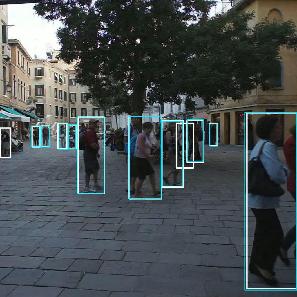
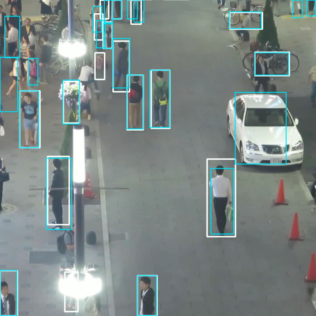
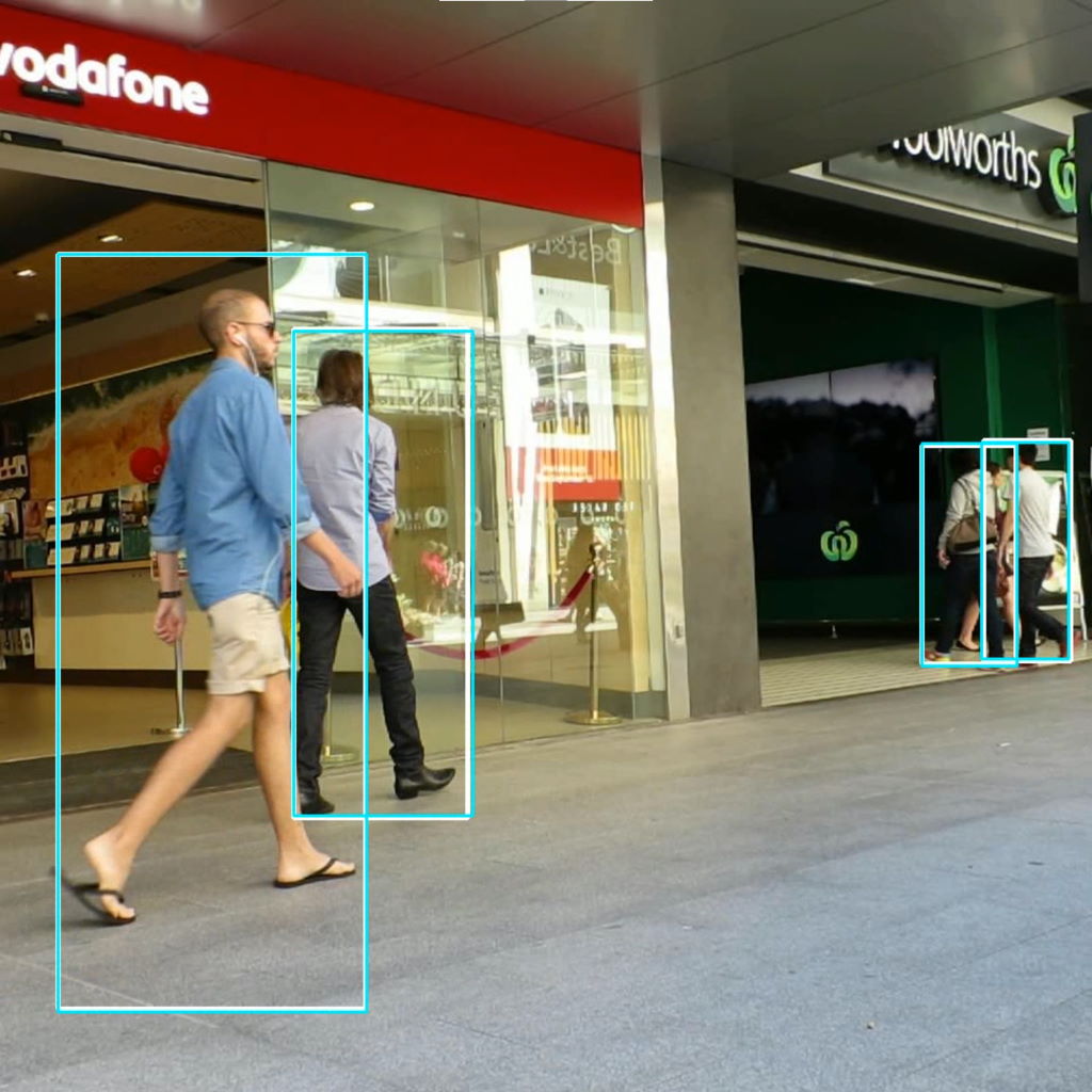
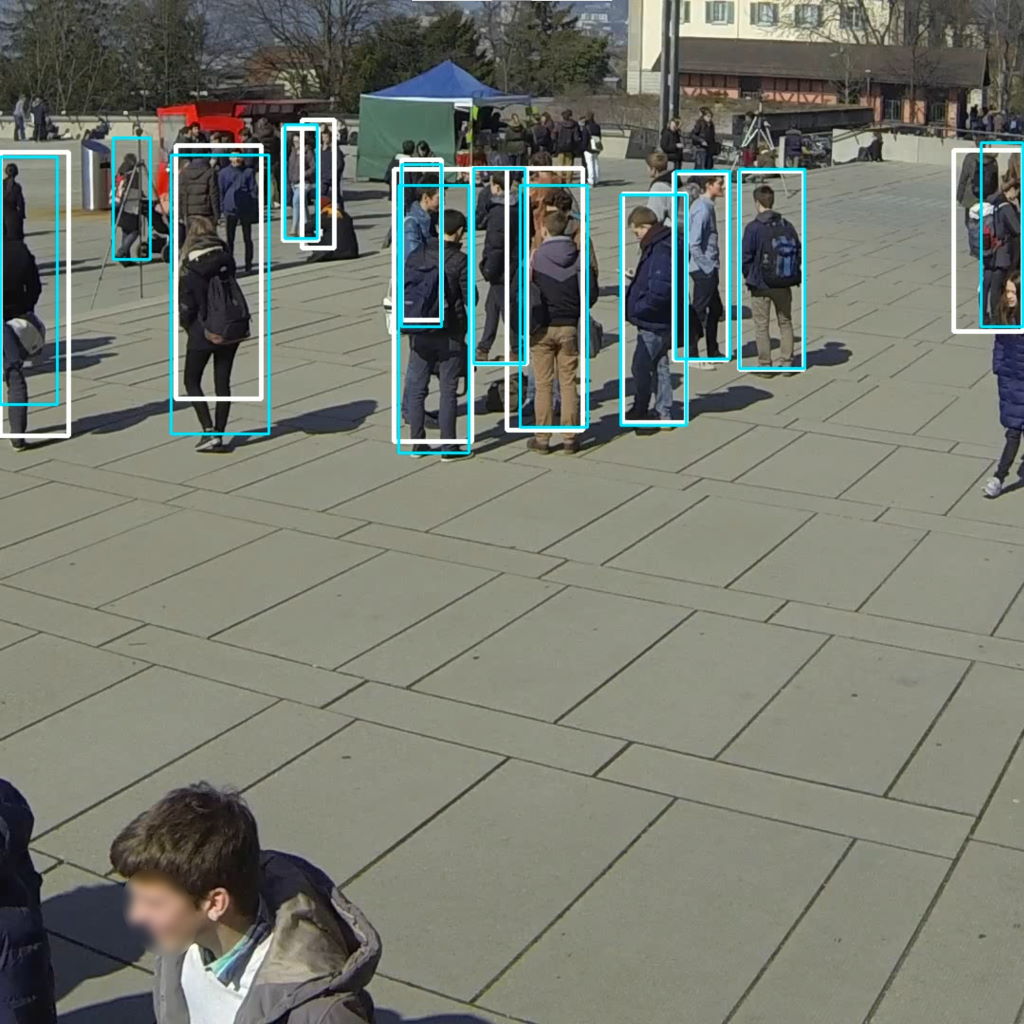
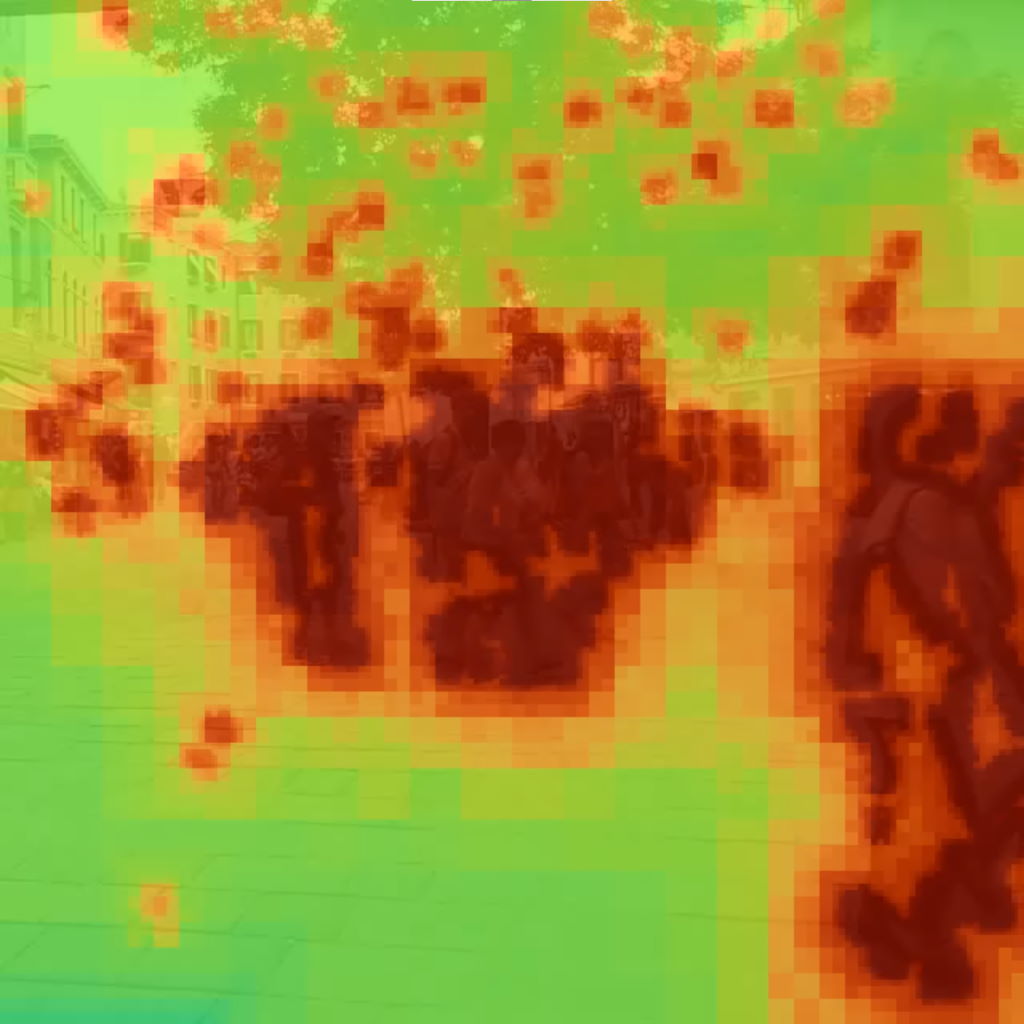
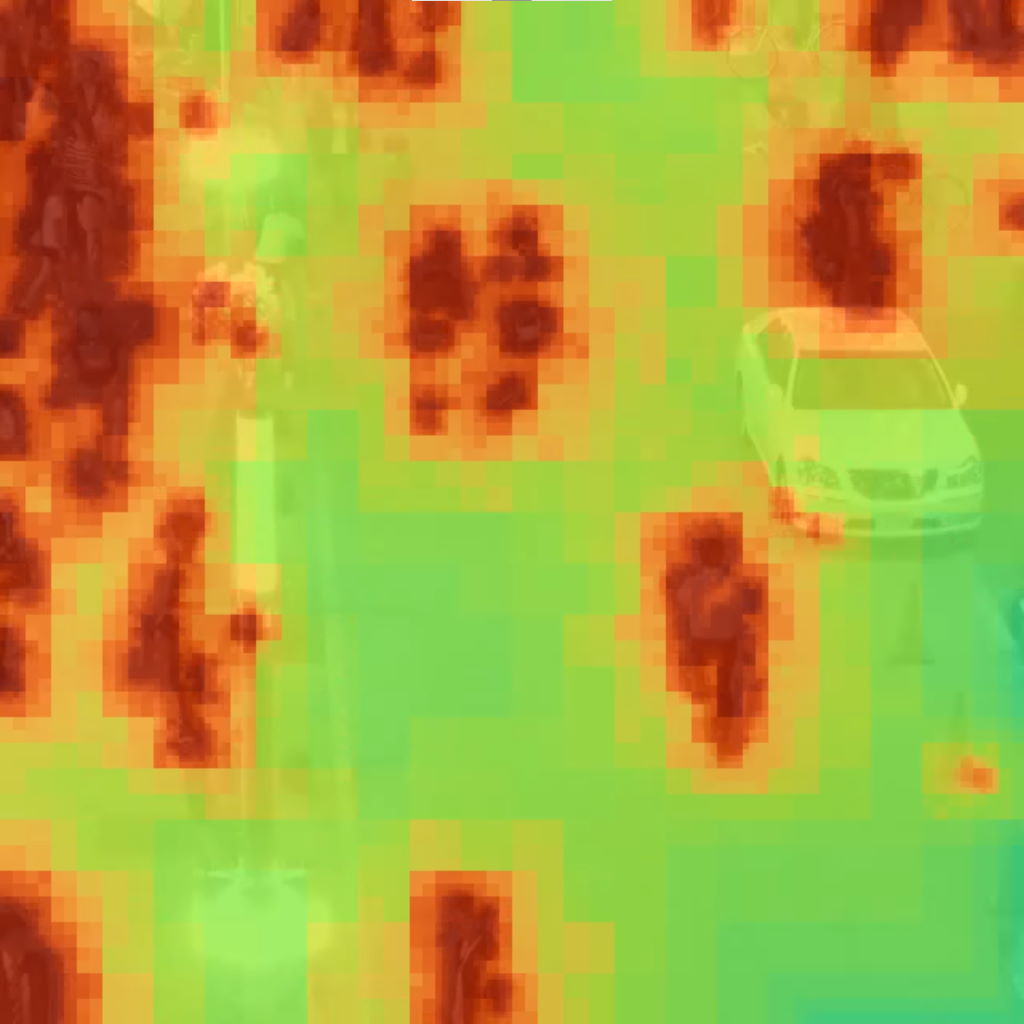
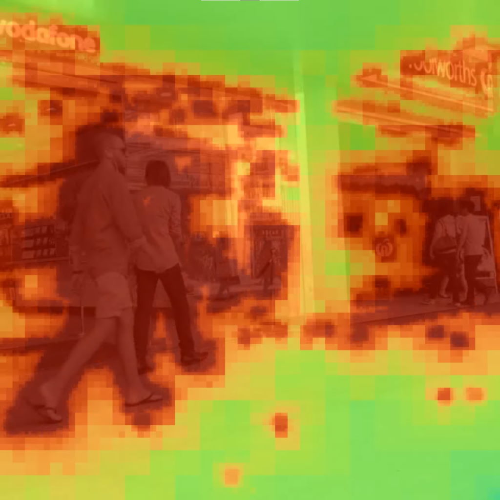
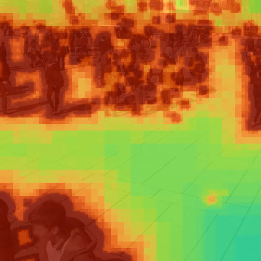
Figure 6: Results using DeltaCNN to accelerate EfficientDet-d1 inference on MOT16 and WildTrack. The first row shows predicted bounding boxes with DeltaCNN (blue) and with the dense reference network (white). The second row shows how many of the convolutional layers updated each pixel.

We evaluate the accuracy versus speedup trade-off for human pose estimation and object detection before analyzing DeltaCNN’s characteristics and side effects of the sparse updates on temporal data.

5.1 Human pose estimation

For human pose estimation, we report accuracy as probability of correct keypoint normalized over head segment length (PCKh) [2] and compare the throughput with different batch sizes. Our results show that DeltaCNN significantly speeds up inference compared to cuDNN and previous work, with marginal loss of accuracy (Table 1). Tuning CBInfer’s thresholds to exactly match the accuracy of our method is difficult and can only be approximated. To emphasize DeltaCNN’s speed advantage, we relaxed the accuracy requirement when tuning the thresholds for CBInfer to allow it to leverage higher levels of sparsity. Even enforcing a much higher accuracy, we still outperform CBInfer speedwise by 3x. It should be mentioned that due to CBInfer’s lack of support for strided, dilated and depth-wise convolutions, 14% of HRNet’s and 7% of Pose-Resnet’s convolutions are processed with the dense cuDNN backend.

We accelerate inference on all tiers of GPUs, with higher speedup on slower devices. High-end GPUs like the RTX 3090 require larger batch sizes to benefit from skipping single tiles. This is because the RTX 3090 has over 10000 compute cores compared to 128 on the Jetson Nano. A batch size of one is typically not large enough to fully utilize the GPU when processing a single low-resolution input image. The surplus of available compute resources for these GPUs means freeing them up by skipping tiles makes little difference.

Detailed evaluations over all frames and kernels for HRNet show that only 6% of input pixels in convolutional layers are updated on average in our approach. 16% of the tiles were processed, resulting in a 84% reduction in FLOPs, and the overall memory transfers are reduced to 21% despite the overhead of reading and updating the additional buffers.

5.2 Object detection

For object detection, we use the Average Precision (AP) metric to measure accuracy. Compared to HRNet and Human3.6M, the EfficientDet model is computationally lightweight and the two datasets contain much denser motion (see Figure 6). Combined, this makes it more difficult to speed up compared to a heavy network and small and centered frame updates. Still, we are able to accelerate inference by a factor of 2.5x to 6.7x over the cuDNN baseline on both datasets and all devices with nearly identical accuracy.

Because CBInfer lacks support for strided and depthwise convolutions (Section 5.1), a third of the layers are processed with the cuDNN backend. CBInfer struggles to accelerate the lightweight network compared to the dense version and is in some cases over 2x slower than cuDNN, even with only 2/3rds of the layers replaced and a 65% reduction in FLOPs.

EfficientDet and EfficientNet provide multiple configurations of the networks (d0-d7) that use different resolutions, layer counts and numbers of channels. This allows us to show that DeltaCNN does not always require trading accuracy for speedup. Instead of using the cuDNN backend for the d0 configuration, DeltaCNN allows for much more accurate predictions (AP@0.5 of 64.0% vs 55.6% on the MOT16 dataset) with the d1 configuration with slightly higher frame rates (+5% on RTX 3090 up to +279% on Jetson Nano).

On the MOT16 dataset, we process nearly 60% of FLOPs of the dense baseline. However, on average, we are able to skip over 60% of the tiles, reducing memory bandwidth by 60%, and thereby achieve over 2x speedup over the dense baseline. Detailed evaluations of accuracy and frame rates for both datasets and both network configurations are reported in the supplementary material.

CNN	Backend	PCKh@0.5	PCKh@0.2	GFLOPs	Jetson Nano		GTX 1050 b=1		GTX 1050 b=4		RTX 3090 b=1		RTX 3090 b=32
					FPS	speedup	FPS	speedup	FPS	speedup	FPS	speedup	FPS	speedup
HRNet	cuDNN	97.29%	87.25%	47.1	0.7	1.0	4.7	1.0	5.2	1.0	10.1	1.0	105	1.0
	ours dense				1.1	1.5	6.8	1.4	7.1	1.4	26.9	2.7	97.6	0.9
	ours $\epsilon=\infty$	28.07%	13.88%	-	6.7	9.6	30.6	6.5	93.7	18.0	31.8	3.1	949	9.0
	CBInfer	96.94%	85.00%	13.9	1.5	2.1	4.9	1.0	10.7	2.1	6.7	0.7	125	1.2
	ours sparse	97.27%	86.33%	7.7	4.7	6.7	20.1	4.3	26.5	5.1	30.5	3.0	433	4.1
ResNet	cuDNN	95.78%	82.79%	27.2	1.5	1.0	7.7	1.0	10.4	1.0	30.4	1.0	215	1.0
	ours dense				1.7	1.1	9.2	1.2	9.8	0.9	63.3	2.1	187	0.9
	ours $\epsilon=\infty$	27.97%	13.77%	-	13.4	8.9	30.8	4.0	42.5	4.1	67.6	2.2	1838	8.5
	CBInfer	95.82%	82.68%	17.6	2.6	1.7	5.6	0.7	16.6	1.6	16.6	0.5	236	1.1
	ours sparse	95.82%	82.68%	11.6	5.7	3.8	20.5	2.7	27.5	2.6	67.4	2.2	577	2.7

Table 1: Speed and accuracy comparisons of different CNN backends used for pose estimation on the Human3.6M dataset. The same set of auto-tuned thresholds for update truncation is used for all devices and batch sizes $b$.

5.3 Additional evaluations

Besides differences in speed and accuracy, temporal reuse and update truncation cause side effects.

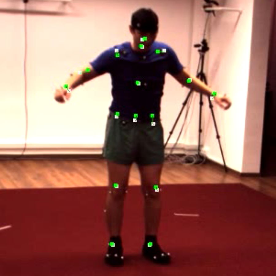
(a) $I^{1}$ dense / ours

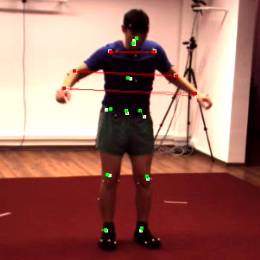
(b) $I^{2}$ dense

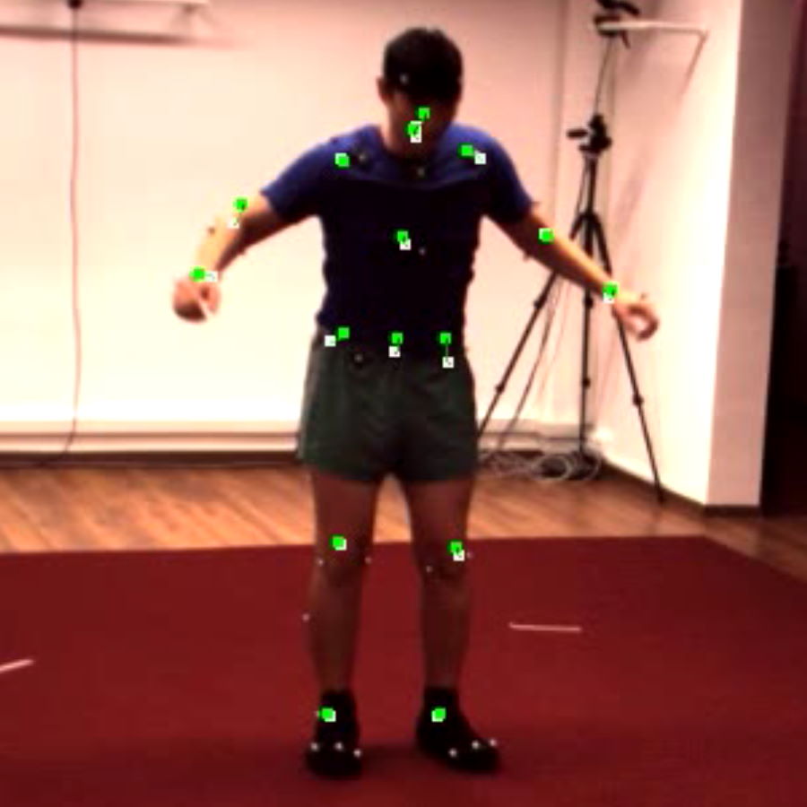
(c) $I^{2}$ ours

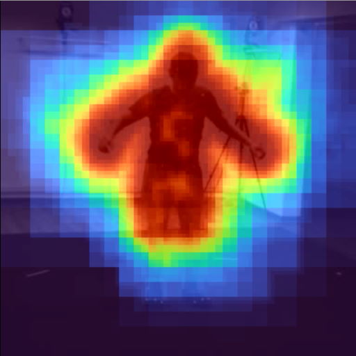
(d) $I^{2}$ updates

Figure 7: DeltaCNN can improve tracking accuracy in some cases due to temporal stability. Here, the dense reference confused left and right arms in frame $I^{2}$, whereas DeltaCNN predicted all joint positions correctly by reusing cached information from $I^{1}$. White, green and red points indicate ground truth, correct and incorrect predictions respectively. Image (d) shows how often a region was updated in $I^{2}$ on average over all HRNet layers using DeltaCNN.

Improved stability When we set the goal of minimizing the number of updates, predictions become more temporally stable and react less to noise in the camera image or by overly sensitive networks. For example, for pose estimation with HRNet, the dense baseline produces 43% more joint position updates compared to DeltaCNN. This effect is especially visible when joints are static, but the dense prediction constantly jitters positions by a few pixels whereas DeltaCNN stays constant (see feet in Figure 7). The temporal stability can even help resolving difficult-to-track poses. Tiny frame-to-frame differences can lead to very different results with dense inference, whereas DeltaCNN mostly relies on information from previous frames and only applies sparse updates (Figure 7).

Threshold analysis Analyzing the tuned thresholds can reveal interesting insights about the contribution of each layer, or about how sensitive layers react to updates on the input. In case of EfficientDet, some branches of the EfficientNet backbone are turned off completely after the first frame, because the frame-by-frame changes do not impact the result. EfficientNet features squeeze and excitation layers, which use average pooling to scale the feature map down to a single pixel. Two convolutions and two activation functions are applied to this pixel before it is used to scale the features of the original feature map. Since average pooling over a sequence of a few seconds returns nearly identical results for all frames, all updates are truncated in the first activation/truncation layer in the squeeze and excitation branch.

Overhead Table 1 shows that DeltaCNN comes with very low overhead. In dense mode, we use negative thresholds to guarantee that all pixels will be reprocessed every time, allowing to compare against cuDNN. Like in sparse mode, we use delta values, accumulated and truncated values buffers and perform all steps including truncation to include all overhead. In most cases, especially for smaller batch sizes, we still outperform cuDNN even when taking the extra steps. This may in part be due to static overheads and different parallelization strategies, leading to DeltaCNN providing more utilization on large GPUs. Yet, these evaluations show that DeltaCNN does not require a minimum level of sparsity to reach the break-even point between overhead and gains.

As DeltaCNN stores accumulated and truncated values, memory overhead scales linearly with batch size and is larger than the memory needed for evaluating the dense version. Recall that memory bandwidth is still reduced by DeltaCNN compared to dense evaluation. Depending on the network architecture, storage overhead can reduce gains when the largest possible batch size is too small to fully utilize the GPU. At the same time, DeltaCNN reduces cache size compared to CBInfer by 28% and 13% with HRNet and EfficientDet.

6 Discussion

Our evaluations show that DeltaCNN can speedup video inference with marginal loss of accuracy. Since DeltaCNN comes with significantly less overhead than previous work, our implementation can accelerate expensive CNNs just like FLOPs-efficient CNNs, datasets with sparse or dense updates and low-end as well as high-end GPUs alike. Thresholds can be tuned to gain identical accuracy with small speedup, or small decreases of accuracy with large speedup. DeltaCNN can even increase the accuracy at the same frame rate by allowing the use of larger networks.

Tiled convolution Our convolutions are processed in tiles, with a single pixel update on the input causing an entire tile to be processed. Compared to CBInfer, this reduces the computational savings for unstructured sparsity, as CBInfer can control sparsity per output pixel. Yet, as the authors of CBInfer stated, frame-to-frame updates are typically structured and per pixel sparsity mainly helps to accelerate the halo of updated regions [3], which contribute only a small portion of the updated pixels. At the same time, our approach achieves state-of-the-art performance for dense inference, allowing us to accelerate even very dense scenes from the MOT16 and WildTrack datasets.

Limitations One major limitation of temporally sparse CNNs, and therefore also of DeltaCNN, is that they only work well on fixed camera input. Even small camera motion can lead to nearly dense updates, at least for the first few layers. Later layers with lower resolution input are often able to truncate parts of the updates, but overall speedup still deteriorates.

Another disadvantage of temporally sparse CNNs is the memory overhead which increases linearly with the batch size. Compared to RRM, Skip-Convolutions and CBInfer, DeltaCNN requires roughly 20% less cache memory. Still, memory can be a limiting factor, especially on low-end devices. If device memory is insufficient, memory overhead could be lowered by omitting delta truncation on some of the activation layers. In this case, the truncated values buffer $x^{T}$ can be avoided at the cost of greater update density.

7 Conclusion

In this paper, we describe DeltaCNN, a method and the corresponding implementation for accelerating CNN inference on video input. DeltaCNN is, to the best of our knowledge, the first solution to offer an end-to-end propagation of sparse frame updates and the first approach of its kind to achieve speedups in practice. With a design optimized for GPUs, we are able to outperform the state-of-the-art framework for dense inference and existing sparse implementations alike. Our approach can be ported to other platforms and processors optimized for CNN acceleration, as the core of the convolution is unaware of sparsity, and speedup is gained by skipping tiles entirely without introducing large processing overhead.

Supplementary Material

In this document, we include the full object detection evaluation table reporting accuracy and speedup in all configurations (see Figure 3). Furthermore, we explain in more detail how the convolutions are implemented to achieve high efficiency (Section 8) and perform ablation studies on threshold tuning (Section 9).

8 Efficient convolution on GPUs

Designing an efficient convolutional layer that is on par with today’s leading framework, cuDNN, requires extensive profiling, analysis and optimizations. Minimization of memory transfers and logic operations, as well as optimizing local memory usage (registers and shared memory) are key in achieving a high performance for compute-heavy operations like convolutions. In this section, we discuss our design decisions and perform ablation studies.

8.1 Tiling for memory reuse

Like cuDNN, we perform convolutions in rectangular tiles. Each tile consists of a few output pixels (4-48, depending on local memory requirements) and is processed by a single cooperative thread array (CTA). Neighboring output pixels share most of their input pixels - in the case of a 3x3 filter, 2 neighboring output pixels share 6 out of each one’s 9 input pixels. Larger tiles lead to better memory reuse and can thereby lower the number of global memory transfers significantly. For example, we use a tile size of 6x6 output pixels for a 3x3 convolutional kernel with a stride of 1. Compared to processing each pixel individually, this reduces the memory reads to less than a fourth, effectively reading less than 2 inputs per output instead of 9. Even more important is the reuse of filter parameters which are often larger than input feature maps. Yet, smaller tile sizes require less registers and allow for more parallelization. And more importantly, smaller tiles are more likely to be skipped as less inputs can require updates. As always, the key is to find the right balance (see Table 2).

8.2 Hybrid dense/sparse tile inference

The convolutional kernel starts with calculating indices, loading the update mask of the input, writing the output mask and, in case any of the inputs was updated, performing the actual convolution. The convolution is performed in three steps: a) load updated input pixels and store them in CTA shared memory and store zero values for inputs which were not updated, b) load filter values and multiply them with the input stored in shared memory, c) write outputs. Steps a) and c) use runtime conditionals against input and output boundaries, update mask and dilation. Step b) uses a highly optimized static code that, independent of the input mask and tile position, always performs all multiply-accumulate operations. Very sparse tiles with four or less active input pixels, making up about 20% of non-empty tiles in our tests, are accelerated in a special mode which can process sparse tiles up to 2x faster. This mode loads only pixels of the filter weights that are required and iterates over an array of active pixels contrary to iterating over all pixels and checking the update flag. The performance impact of adding a runtime conditional to allow for per-pixel sparsity (check each pixel if processing is required) and the performance of our hybrid approach compared to a per-tile sparsity (process all pixels or none) approach are reported in Table 2.

It should be noted that depth-wise convolutions require a special implementation to stay competitive against cuDNN. In depth-wise convolutions, every output channel only depends on input values of the corresponding channel in the input feature map. Because of that, input values are used less often and (in our implementation) only by a single thread, removing the necessity of keeping data local to a CTA. When loading input data, the update flag of a pixel must always be checked before reading the values because non-updated pixels contain invalid data. Since the loaded value is only used for up to 9 multiplications in the case of a 3x3 convolution, we fuse loading and multiplication steps described above. Thus, we decide per pixel if we load the value and perform the multiplication – resulting in a per-pixel sparse operation compared to per-tile for standard convolutions. Still, skipping a tile entirely is much faster than processing a single input pixel.

Tile Mode	Tile Size	s=0%	s=50%	s=90%	s=99%
p.t. Sparse	6x6	17.0	16.9	16.5	7.7
	5x5	23.7	23.6	22.9	8.5
Hybrid	6x6	17.0	16.9	15.8	5.0
	5x5	23.5	23.2	18.3	4.5
p.p. Sparse	6x6	60.4	51.9	44.3	20.4
	5x5	49.6	43.6	38.0	14.1

Table 2: GTX 1050 runtime comparison between different tile sizes and sparsity levels ($s$) reported in milliseconds for a 3x3 convolution with 128 input and output channels and a 256x256 pixels input. Since sparsity is generated uniformly, even with a 90% sparse input is very likely have at least one updated pixel per tile. Per-tile sparse mode always processes either all pixels of a tile or none of them. Per-pixel sparse mode decides per input pixel whether it needs to be processed or can be skipped. Hybrid mode uses dense mode when more than four input pixels are updated and uses a special implementation for very sparse tiles. Larger tile sizes cannot be used due to local memory resource limitations.

8.3 Memory layout for bandwidth reductions

Using a per-pixel update mask, we can reduce the memory bandwidth during inference greatly in many ways. Compared to previous work that had to compare the inputs of each layer against previous values, we only load values that were marked as updated. Furthermore, using the update mask, we do not have to set unchanged values in the feature map to zero. This allows us to use uninitialized memory for the greater part of the feature maps - only writing valid values for updated pixels. Compared to setting all unchanged output features to zero, this improved the performance of convolutions in HRNet by up to 68%.

PyTorch’s default memory layout is $NCHW$, storing one image per pixel channel. Accessing pixels individually, however, is very inefficient with this layout, as the minimum memory access size – a cache line – would always load multiple neighboring pixels per instruction. For efficient use of per-pixel sparsity, we store feature maps in $NHWC$ format. This way, all channels of a pixel are stored coalesced and can be accessed efficiently.

8.4 Floating point number inaccuracies

While delta updates can in theory be applied indefinitely, floating point number operations result in slightly different outcomes when taking large accumulated values or small deltas as input. With HRNet and Human3.6M, we did not experience any problems even with sequences thousands of frames long. However, we did notice small errors accumulating over time in EfficientDet, even with dense inference, i.e. using negative thresholds. We recommend to reset the buffers every few hundred frames, or when the network input switches between different videos, to flush all accumulated errors due to floating point inaccuracies.

9 Threshold tuning ablation study

In our evaluations, we used a maximum loss increase target of 3% for the task of threshold tuning. To ensure that we do not exceed this limit, every truncation threshold is only allowed to increase the loss by a maximum of $\frac{3\%}{\#_{layers}}$. Due to a predefined step size in the threshold tuning process, however, the actual loss increase is typically much lower. We evaluated different maximum loss increase targets to compare the resulting accuracy and speedup (see Figure 8). To better show the impact of different parameters, we do not use a high threshold and update mask dilation on the first layer as this already increases sparsity greatly, and thereby reduces the impact of the chosen parameters. Instead, we set the first threshold to a low value of 0.15 manually.

Figure 8: Accuracy and speedup achieved with EfficientDet-d1 on the MOT16 dataset with thresholds tuned on different maximum loss increase targets. Even when using a 30% total loss increase target, the accuracy stays close to dense inference. With a smaller step size for threshold tuning, the accuracy could be kept closer to the maximum loss increase target.

9.1 Training truncation thresholds

We experimented with training truncation thresholds in parallel instead of auto-tuning them one-by-one. Using the update mask density as an additional loss, the trade-off between accuracy and pixel update density could be optimized more accurately and the accuracy reduction per layer could be better balanced. E.g. early layers of the CNNs can be allowed a larger accuracy decrease, because they have a larger impact on the overall update density.

Instead of boolean update masks, we used soft truncation with a sigmoid activation function to allow for gradients to propagate better. With the same intention, we switched to using norm truncation instead of maximum truncation, i.e. we compare the $L^{2}$ norm of a pixel’s deltas against a threshold. This way, all values contribute to the update mask and the training process is more stable than with maximum truncation. While we managed to train feasible thresholds with a pre-defined accuracy vs. sparsity trade-off, the resulting thresholds did not outperform tuned thresholds. Furthermore, threshold training takes many times longer to process and hyper parameters are more difficult to tune than the single parameter used for auto tuning.

Dataset	Backend	AP@0.5	AP@.5:.95	GFLOPs	Jetson Nano b=1		GTX 1050 b=1		GTX 1050 b=8/3		RTX 3090 b=1		RTX 3090 b=48/24
					FPS	speedup	FPS	speedup	FPS	speedup	FPS	speedup	FPS	speedup
MOT16-d0	cuDNN	55.6%	27.8%	5.0	1.4	1.0	26.0	1.0	26.4	1.0	29.3	1.0	368	1.0
	ours dense				4.0	2.9	29.3	1.1	28.6	1.1	57.2	2.0	369	1.0
	ours $\epsilon=\infty$	17.9%	6.6%	-	8.8	6.3	61.0	2.4	340	12.9	57.0	2.0	2389	6.5
	CBInfer	54.3%	27.0%	1.7	2.0	1.4	9.5	0.4	24.3	0.9	15.6	0.5	273	0.7
	ours sparse	55.8%	27.8%	2.8	7.9	5.6	48.2	1.9	76.6	2.9	57.2	2.0	896	2.4
MOT16-d1	cuDNN	63.9%	32.2%	12.2	0.7	1.0	10.5	1.0	11.3	1.0	23.3	1.0	169	1.0
	ours dense				1.8	2.6	11.6	1.1	11.8	1.0	45.0	1.9	167	1.0
	ours $\epsilon=\infty$	21.7%	7.2%	-	6.6	9.4	51.1	4.9	151.6	13.4	44.0	1.9	1032	6.1
	CBInfer	63.5%	31.9%	4.6	1.3	1.9	6.3	0.6	9.4	0.8	11.4	0.5	106	0.6
	ours sparse	64.0%	32.0%	6.8	3.9	5.6	27.4	2.6	30.9	2.7	45.2	1.9	389	2.3
WildTrack-d0	cuDNN	67.1%	35.4%	5.0	1.4	1.0	26.0	1.0	26.4	1.0	29.3	1.0	383	1.0
	ours dense				4.0	2.9	29.3	1.1	28.6	1.1	57.2	2.0	384	1.0
	ours $\epsilon=\infty$	29.5%	14.3%	-	8.8	6.3	61.0	2.4	340	12.9	57.0	2.0	2389	6.5
	CBInfer	65.4%	33.9%	1.1	2.2	1.6	10.4	0.4	25.0	0.9	16.8	0.6	274	0.7
	ours sparse	66.4%	34.7%	2.3	8.1	5.8	56.1	2.2	100	3.8	57.2	2.0	973	2.5
WildTrack-d1	cuDNN	72.1%	41.6%	12.2	0.7	1.0	10.5	1.0	11.3	1.0	23.3	1.0	169	1.0
	ours dense				1.8	2.6	11.6	1.1	11.8	1.0	45.0	1.9	167	1.0
	ours $\epsilon=\infty$	28.3%	15.0%	-	6.6	9.4	51.1	4.9	151	13.4	45.9	2.0	1032	6.1
	CBInfer	71.5%	40.5%	2.4	1.4	2.0	6.8	0.6	10.6	0.9	13.1	0.6	120	0.7
	ours sparse	71.6%	40.8%	5.7	4.8	6.9	32.1	3.1	38.6	3.4	44.8	1.9	415	2.5

Table 3: Speed and accuracy comparisons of different CNN backends used for the task of object detection with batch size $b$. MOT16 is evaluated only on fixed camera videos. Our evaluations show that DeltaCNN achieves higher frame rate and accuracy using the 12.2 GFLOPs d1 configuration of EfficientDet than cuDNN achieves with the 5.0 GFLOPs d0 configuration.

References

- [1] Udari De Alwis and Massimo Alioto. TempDiff: Temporal Difference-Based Feature Map-Level Sparsity Induction in CNNs with <4% Memory Overhead. 2021 IEEE 3rd International Conference on Artificial Intelligence Circuits and Systems, AICAS 2021, pages 1–4, Jun 2021.
- [2] Mykhaylo Andriluka, Leonid Pishchulin, Peter Gehler, and Bernt Schiele. 2D human pose estimation: New benchmark and state of the art analysis. Proceedings of the IEEE Computer Society Conference on Computer Vision and Pattern Recognition, pages 3686–3693, 2014.
- [3] Lukas Cavigelli and Luca Benini. CBinfer: Exploiting Frame-to-Frame Locality for Faster Convolutional Network Inference on Video Streams. IEEE Transactions on Circuits and Systems for Video Technology, 30(5):1451–1465, May 2020.
- [4] Tatjana Chavdarova, Pierre Baque, Stephane Bouquet, Andrii Maksai, Cijo Jose, Timur Bagautdinov, Louis Lettry, Pascal Fua, Luc Van Gool, and Francois Fleuret. WILDTRACK: A Multi-camera HD Dataset for Dense Unscripted Pedestrian Detection. Proceedings of the IEEE Computer Society Conference on Computer Vision and Pattern Recognition, pages 5030–5039, 2018.
- [5] Yunji Chen, Tianshi Chen, Zhiwei Xu, Ninghui Sun, and Olivier Temam. DianNao family: Energy-efficient hardware accelerators for machine learning. Communications of the ACM, 59(11):105–112, 2016.
- [6] Yunji Chen, Tao Luo, Shaoli Liu, Shijin Zhang, Liqiang He, Jia Wang, Ling Li, Tianshi Chen, Zhiwei Xu, Ninghui Sun, and Olivier Temam. DaDianNao: A Machine-Learning Supercomputer. Proceedings of the Annual International Symposium on Microarchitecture, MICRO, 2015-January:609–622, Jan 2015.
- [7] Patrick Dendorfer, Aljosa Osep, Anton Milan, Konrad Schindler, Daniel Cremers, Ian Reid, Stefan Roth, and Laura Leal-Taixé. MOTChallenge: A Benchmark for Single-Camera Multiple Target Tracking. International Journal of Computer Vision, 129(4):845–881, 2021.
- [8] Jia Deng, Wei Dong, Richard Socher, Li-Jia Li, Kai Li, and Li Fei-Fei. ImageNet: A large-scale hierarchical image database. pages 248–255, Mar 2010.
- [9] Zhipeng Fan, Jun Liu, and Yao Wang. Adaptive Computationally Efficient Network for Monocular 3D Hand Pose Estimation. Technical report, 2020.
- [10] Benjamin Graham, Martin Engelcke, and Laurens Van Der Maaten. 3D Semantic Segmentation with Submanifold Sparse Convolutional Networks. Proceedings of the IEEE Computer Society Conference on Computer Vision and Pattern Recognition, pages 9224–9232, Nov 2018.
- [11] Amirhossein Habibian, Davide Abati, Taco S. Cohen, and Babak Ehteshami Bejnordi. Skip-Convolutions for Efficient Video Processing. In Proceedings of the IEEE/CVF Conference on Computer Vision and Pattern Recognition (CVPR), pages 2695–2704, Jun 2021.
- [12] Song Han, Xingyu Liu, Huizi Mao, Jing Pu, Ardavan Pedram, Mark A. Horowitz, and William J. Dally. EIE: Efficient Inference Engine on Compressed Deep Neural Network. Proceedings - 2016 43rd International Symposium on Computer Architecture, ISCA 2016, pages 243–254, 2016.
- [13] Song Han, Jeff Pool, John Tran, and William J. Dally. Learning both weights and connections for efficient neural networks. Advances in Neural Information Processing Systems, 2015-January:1135–1143, 2015.
- [14] Itay Hubara, Matthieu Courbariaux, Daniel Soudry, Ran El-Yaniv, and Yoshua Bengio. Quantized neural networks: Training neural networks with low precision weights and activations. Journal of Machine Learning Research, 18:1–30, 2018.
- [15] Catalin Ionescu, Dragos Papava, Vlad Olaru, and Cristian Sminchisescu. Human3.6M: Large scale datasets and predictive methods for 3D human sensing in natural environments. Technical Report 7, 2014.
- [16] Samvit Jain, Xin Wang, and Joseph E. Gonzalez. Accel: A corrective fusion network for efficient semantic segmentation on video. Proceedings of the IEEE Computer Society Conference on Computer Vision and Pattern Recognition, 2019-June:8858–8867, Jun 2019.
- [17] Athindran Ramesh Kumar, Balaraman Ravindran, and Anand Raghunathan. Pack and detect: Fast object detection in videos using region-of-interest packing. ACM International Conference Proceeding Series, pages 150–156, 2019.
- [18] CUN Le. Optimal brain damage. Advances in Neural Information Processing Systems, 2:598–605, 1990.
- [19] Yule Li, Jianping Shi, and Dahua Lin. Low-Latency Video Semantic Segmentation. Proceedings of the IEEE Computer Society Conference on Computer Vision and Pattern Recognition, pages 5997–6005, 2018.
- [20] Darryl D. Lin, Sachin S. Talathi, and V. Sreekanth Annapureddy. Fixed point quantization of deep convolutional networks. 33rd International Conference on Machine Learning, ICML 2016, 6:4166–4175, 2016.
- [21] Tsung Yi Lin, Michael Maire, Serge Belongie, James Hays, Pietro Perona, Deva Ramanan, Piotr Dollár, and C. Lawrence Zitnick. Microsoft COCO: Common objects in context. Lecture Notes in Computer Science, 8693 LNCS(PART 5):740–755, 2014.
- [22] Bert Moons, Koen Goetschalckx, Nick Van Berckelaer, and Marian Verhelst. Minimum energy quantized neural networks. Conference Record of 51st Asilomar Conference on Signals, Systems and Computers, ACSSC 2017, 2017-October:1921–1925, Apr 2018.
- [23] Xuecheng Nie, Yuncheng Li, Linjie Luo, Ning Zhang, and Jiashi Feng. Dynamic kernel distillation for efficient pose estimation in videos. Proceedings of the IEEE International Conference on Computer Vision, 2019-October:6941–6949, Oct 2019.
- [24] Bowen Pan, Wuwei Lin, Xiaolin Fang, Chaoqin Huang, Bolei Zhou, and Cewu Lu. Recurrent Residual Module for Fast Inference in Videos. Technical report, 2018.
- [25] Gao Peng, Bo Pang, and Cewu Lu. Efficient 3D Video Engine Using Frame Redundancy. In Proceedings of the IEEE/CVF Winter Conference on Applications of Computer Vision (WACV), pages 3792–3802, Jan 2021.
- [26] Mengye Ren, Andrei Pokrovsky, Bin Yang, and Raquel Urtasun. SBNet: Sparse Blocks Network for Fast Inference. Technical report, 2018.
- [27] Evan Shelhamer, Kate Rakelly, Judy Hoffman, and Trevor Darrell. Clockwork convnets for video semantic segmentation. Lecture Notes in Computer Science (including subseries Lecture Notes in Artificial Intelligence and Lecture Notes in Bioinformatics), 9915 LNCS:852–868, 2016.
- [28] Laurent Sifre and Stéphane Mallat. PhD Thesis, Ecole Polytechnique, CMAP Rigid-Motion Scattering For Image Classification. 2014.
- [29] Ke Sun, Bin Xiao, Dong Liu, and Jingdong Wang. Deep high-resolution representation learning for human pose estimation. Proceedings of the IEEE Computer Society Conference on Computer Vision and Pattern Recognition, 2019-June:5686–5696, 2019.
- [30] Mingxing Tan and Quoc V. Le. EfficientNet: Rethinking model scaling for convolutional neural networks. Technical report, 2019.
- [31] Mingxing Tan, Ruoming Pang, and Quoc V. Le. EfficientDet: Scalable and efficient object detection. Proceedings of the IEEE Computer Society Conference on Computer Vision and Pattern Recognition, pages 10778–10787, 2020.
- [32] Bin Xiao, Haiping Wu, and Yichen Wei. Simple baselines for human pose estimation and tracking, 2018.
- [33] Xizhou Zhu, Jifeng Dai, Lu Yuan, and Yichen Wei. Towards High Performance Video Object Detection. Proceedings of the IEEE Computer Society Conference on Computer Vision and Pattern Recognition, pages 7210–7218, 2018.
- [34] Xizhou Zhu, Yuwen Xiong, Jifeng Dai, Lu Yuan, and Yichen Wei. Deep feature flow for video recognition. Proceedings - 30th IEEE Conference on Computer Vision and Pattern Recognition, CVPR 2017, 2017-January:4141–4150, 2017.