Can Chameleon fields be the source of both the dark energy dipole and the CMB dipole?

Abstract

Recent research shows that the local group is moving toward $(l,b)=(276,30)$ relative the cosmic background radiation at a speed of about $600kms^{-1}$ which is known as the cosmic background radiation dipole.The exact cause of this movement is still unknown. Areas with high mass densities such as galactic superclusters seem to be one of the causes of this flow.There are several methods for simulating the motion of local clusters,one of which is the bulk flow .The bulk current can be seen as a mass movement of a large part of the universe.This anisotropy at local scale, seems to have the same origin as the anisotropy at the larger scale.In this paper, anisotropies on both small and large scales were investigated using chameleon fields.The data used are Type Ia supernovae (Pantheon catalog for a total of 1,048 supernovae in redshift (0.15<z<2.3)).The results showed that on a smaller scale (less than 150 MPa) the direction of motion of the local group galaxies is the same as the direction of the bulk, and on larger scales, the direction of the bulk current is the same as the direction of the current of dark energy dipole.

1 Introduction

With the studies carried out on cosmic background anisotropy by Conklin in 1969(Conklin, 1969) Henry in 1971(Henry, 1971), and Smoot et al. In 1977(Smoot et al, 1977), the best justification for this anisotropy was the movement of local group galaxies toward cosmic background radiation, which is called cosmic background radiation diploe or CMB diploe,which is a more famous term. Immediately, many studies were conducted to measure the exact amount of local cluster velocity and the cause of this movement. Initial assumptions were that the Virgo supercluster, located approximately 17 megaparsecs from the local group galaxy, was responsible for the move. However, studies by Villumsen and Strauss in 1987(Villumsen & Strauss, 1987) showed that a high-density mass distribution over long distances was needed to justify the motion of a local cluster. Studies done by Shaya in 1984(Shaya, 1984) , Tammann in 1985(Tammann & andSandage, 1985), and Aronson et al.(Aaronson et al, 1986) in 1986 illustrated that the difference in direction between the CMB dipole and the stream flowing, toward the center of Virgo in the direction of the Hydra-Centauri superclusters is approximately 32 MPa; As a result they reported that this supercluster attracts the local cluster. In 1987, Dressier et al.(Dressier et al, 1987) studied the motion of the galaxies of the Hydra-Centaurus cluster and showed that the cluster was moving at a speed of approximately 500 $kms^{-1}$ relative to the background radiation. As a result, this supercluster cannot be the only cause of local cluster motion, and a large mass distribution over a longer distance must be the source of this motion. Linden-Bell et al. (1988)(Lynden-Bell et al, 1988) then investigated the motion of 400 spiral galaxies that covered all angles of the sky, showing that these galaxies were moving toward a massive mass called the Great Attractor at a distance of 50-70$h^{-1}Mpc$. The galactic coordinates are $(l,b)=(325,-7.25)$, flowing. In 1992, Bothun et al.(Bothun et al, 1992) studied 48 spiral galaxies adjacent to the Great Attractor using the Tully-Fisher relation to demonstrate that these galaxies were moving toward the Great Attractor. After the first Kobe satellite results were published, accurate measurements of the speed of the local group galaxy were carried out by Kogut et al.(Kogut et al, 1993) in 1993. Using the first data from the satellite, they estimated the speed of the local group at $627kms^{-1}$. With the development of catalogs such as $(2MASS)$ for galactic coordinates $(l,b)=(276^{+3}_{-3},30^{+3}_{-3})$, Hoffman et al.(Hoffman et al, 2001) 2001, and Kocevski and Abiling 2006(Kocevski et al, 2006) studies indicated that to reconstruct the local group’s dipole motion, the local group must be studied for distances farther away from the Shapely supercluster at 150$h^{-1}Mpc$. Although studies conducted up to 2008 have had a good convergence in the reconstruction of the motion of the local group galaxy, these results usually revealed a directional difference of 10 to 30 degrees.On the other hand, studies that sought to find the direction of motion of local group galaxies using the peculiar velocity of galaxies; did not reach a definite conclusion to justify the motion of local group galaxies; they concluded,however, that galaxy clusters posed a collective and cohesive movement and that they have a certain direction to the cosmic background radiation called the bulk current. Until 2008, studies were conducted at depths of 150$h^{-1}Mpc$, but in 2008(k et al, 2008), Kashlinsky, Atrio-Barandela, Kocevski and Ebeling analyzed three-year WMAP data, the cinematic use of Sunyaev–Zeldovich’s data, and data covering up to 300$h^{-1}Mpc$, and provide some evidence. The coordinated motion and coherent flow of galaxy clusters at speeds of 600-1000 $kms^{-1}$ were found in the direction of the galaxy coordinates, which were close to the constellations Centaurus and Vela. Researchers have speculated that the move maybe a remnant of the impact of pre-inflation invisible areas of the world. In 2009 and 2010, the results obtained by Kashlinsky et al.(k1 et al, 2009)-(k2 et al, 2010) were corrected by Watkins, Feldman, and Hudson, and they achieved a velocity of $(l,b)=(282^{+11}_{-11},6^{+6}_{-6})$. In 2013, data from the Planck Space Telescope showed no evidence of dark currents at this scale, and claims denied the evidence of gravitational effects beyond the visible universe. Using Planck and WMAP’s data, they have seen evidence of dark currents; thus, studies on finding the direction of motion of galaxies in the local group have posed a newer enigma called the bulk flow, for which a definitive answer has not been determined yet. Most studies of bulk flow pursue three main goals: 1. Calculate the direction and size of the bulk speed 2. The degree of convergence of the velocity of the bulk with the direction of motion of the galaxies of the local group 3. Investigating the degree of convergence for the motion of the bulk and the motion of the galaxies of the local group with supergroups such as Virgo, Hydra, Centaurus, Coma and Shapley because it is thought that these supergroups which are located at different distances are the source of the bulk current and the direction of local cluster motion. In this paper, in addition to the above, we determine the range of parameters of the Chameleon model using the bulk current and the degree of convergence of the bulk current with the dipole direction of dark energy.

2 Theoretical model

As mentioned, the bulk current can be seen as a coherent and coordinated motion of a large part of the universe. This motion involves the mass movement of galaxies, galaxy clusters, supernovae, and other cosmic objects relative to a frame of reference (usually cosmic background radiation). Different definitions and formulations of bulk velocity have been reported that may seem different in appearance but are fundamentally the same. Nusser et al.(Nusser & Davis, 2011) have put forwards a way to determine the velocity of the bulk through the following equation:

$$B(r)=\frac{3}{4\pi r^{3}}\int_{x<r}v(x)d^{3}x,$$ (1)

$v(x)$ is the peculiar velocity of objects within the volume of the sphere under study with radius $r$. More often than not different samples such as galaxy clusters and supernovae are studied. Although it is expected to measure the velocity of the bulk for all samples, they lead to almost the same answer; notwithstanding the more uniform the sample distribution, the less computational error, and different methods and catalogs for measuring the velocity of the bulk. The peculiar motion of supernovae causes changes in their luminosity distance and oscillations in their luminosity distance, which is expressed by the following formula:(Bon et al, 2006)

$$d_{L}(z,\upsilon_{DF},\theta)=d^{0}_{L}(z)+d^{dipole}_{L}(z,\upsilon_{DF},\theta),$$ (2)

Where $d^{0}_{L}(z)$ is the luminosity distance of the supernova and obtained from the following relation:

$$d^{0}_{L}(z)=c(1+z)\int^{z}_{0}\frac{dz^{\prime}}{H(z^{\prime})},$$ (3)

.

In the above relation, $H(z)$, the Hubble parameter and $z$ redshift, $\upsilon_{DF}$ are the velocity of the bulk and $d^{(dipole)}_{L}(z,\upsilon_{DF},\theta)$ is the dipole domain of the velocity of bulk, which is obtained from the following equation:

$$d^{(dipole)}_{L}(z,\upsilon_{DF},\theta)=\frac{\upsilon_{DF}(1+z)^{2}}{H(z)}.\cos(\theta).$$ (4)

Where $\theta$ is the angle between the supernova line of sight and the dipole direction (bulk flow direction). It should be noted that the luminosity interval may be disturbed for other reasons, but other sources of disturbance are important in redshift greater than 1.(Hui & Patrick, 2006) Considering that in this article we have used 211 supernovae that are less than 0.1 in redshift, other sources of disturbance can be omitted. It is important to note that although the bipolar fitting method (so-called dipole fit) seems to be a model-independent method, looking at the equation, it can be seen that this method is completely similar to the cosmological model through the Hubble parameter. Because the evolution of the Hubble parameter depends on the cosmological model and this parameter is one of the most basic cosmic parameters that is analyzed and fitted in different models both directly and through other parameters that are related to this parameter.

3 Chameleon fields

Evidence for the accelerated expansion of the universe and time-dependent changes in the micro structure has led to the introduction of a scalar field with mass $H_{0}$, which is the current Hubble constant value. If such a field exists, it must be paired with matter in order to satisfy the principle of equivalence. In 2003, Justin Khoury and Amanda Weltman(Khoury & Weltman, 2004) studied these fields and contented that the mass associated with these fields depends on the local density of matter in the universe. They also showed that the interaction range of these fields on Earth is about $1mm$ and on scale of the solar system is of the order of $10-10^{4}AU$. In these studies, all the boundaries and principles of general relativity have been entered, and it is predicted that Newton fixed measurement probes such as the SEE will achieve a value of a single order of magnitude at its present value on Earth in the future. Considering the normalized action of Hilbert-Einstein as:

$$S_{EH}=\int d^{4}x\sqrt{-g}\frac{1}{16\pi G}R=\int d^{4}x\sqrt{-g}\frac{M_{pl}^{2}}{2}R,$$ (5)

In the presence of a scalar field $\phi$ and potential $V(\phi)$, another sentence as:

$$S_{\phi}=-\int d^{4}x\sqrt{-g}\left\{\frac{1}{2}(\partial\phi)^{2}+V(\phi)\right\}.$$ (6)

is added to the action. To introduce Chameleon fields, a set of fields $\psi_{m}^{(i)}$ by action:

$$S_{m}=-\int d^{4}x\mathcal{L}_{m}\left(\psi_{m}^{(i)},g_{\mu\nu}^{(i)}\right),$$ (7)

which are coupled to scalar field $\phi$ , is added to them. In these relationships:

$$g_{\mu\nu}^{(i)}\equiv e^{2\beta_{i}\phi/M_{pl}}g_{\mu\nu},$$ (8)

$\beta_{i}$ is also a coupling constant for every small element of matter. So the total action is expressed as follows:

$$S=\int d^{4}x\sqrt{-g}\left\{\frac{M_{pl}^{2}}{2}R-\frac{1}{2}\left(\partial\phi\right)^{2}-V(\phi)\right\}-\int d^{4}x\mathcal{L}_{m}\left(\psi_{m}^{(i)},g_{\mu\nu}^{(i)}\right)\\$$ (9)

as a result

$$S=\int d^{4}x\sqrt{-g}\left\{\frac{M_{pl}^{2}}{2}R-\frac{1}{2}\nabla_{\mu}\phi\nabla^{\mu}\phi-V(\phi)-\frac{1}{\sqrt{-g}}\mathcal{L}_{m}\left(\psi_{m}^{(i)},g_{\mu\nu}^{(i)}\right)\right\}.$$ (10)

$\phi$, the equation of motion of the Chameleons is obtained as follows:

$$\nabla^{2}\phi=V_{{eff},\phi}(\phi).$$ (11)

For a non-relativistic matter$(w_{i}\approx 0)$, the effective potential is simplified by the following equation:

$$V_{{eff}}(\phi)=V(\phi)+\sum_{i}\rho_{i}e^{\beta_{i}\phi/M_{pl}}.$$ (12)

Since exponential potentials play an important role in describing the period of inflation,(Ferreira & Joyce, 1998)-(Wetterich, 1988) we examine the Chameleon field equations in the presence of potential $V=V_{0}\exp\big{(}-\alpha\frac{\phi}{M_{pl}}\big{)}$. Here $\alpha$, is a dimensionless constant that describes the potential slope. The Chameleon field equation in the presence of exponential potential is obtained as follows:

$$\ddot{\phi}+3H\dot{\phi}=\frac{V_{0}\alpha}{M_{pl}}e^{\frac{-\alpha}{M_{pl}}\phi}-\frac{\beta}{M_{pl}}\rho_{m}e^{\frac{\beta}{M_{pl}}\phi},$$ (13)

Here $H$ is the Hubble parameter which is determined by the Friedmann constraint as follows:

$$3H^{2}M_{pl}^{2}=\frac{1}{2}\dot{\phi}^{2}+V_{0}e^{\frac{-\alpha}{M_{pl}}\phi}+\rho_{m}e^{\beta\phi/M_{pl}}$$ (14)

$$(2\dot{H}+3H^{2})M_{pl}^{2}=-\frac{1}{2}\dot{\phi}^{2}+V_{0}e^{\frac{-\alpha}{M_{pl}}\phi}-\gamma\rho_{m}e^{\beta\phi/M_{pl}}$$ (15)

The effective energy density in the Chameleon field is $\rho_{eff}=\frac{1}{2}\dot{\phi}^{2}+V\left(\phi\right)+\rho_{m}e^{\beta\phi/M_{pl}}$ and the effective pressure is $P_{eff}=-\frac{1}{2}\dot{\phi}^{2}+V\left(\phi\right)$. In the previous studies, important parameters $(\alpha,\beta)$ in Chameleon field have been investigated and the range of these parameters has been fitted with observational tests(Farajollahi & Salehi, 2012). These two parameters play an essential role in the dynamics of the universe. Another feature of these two parameters is that the stability range of critical states of the Chameleon model is determined by these parameters. The above equations are a nonlinear set of second-order differential equations whose analytical solution is possible only for certain cases. Therefore, they can be examined in terms of numerical calculations. In this article, these variables are defined as follows:

$$\varTheta={\frac{\rho_{m}e^{\frac{\beta\phi}{M_{pl}}}}{3H^{2}M_{pl}^{2}}},\ \ \varUpsilon=\frac{\dot{\phi}}{\sqrt{6}HM_{pl}},\ \ \zeta=\frac{V}{3H^{2}M_{pl}^{2}}.$$ (16)

Friedman’s constraint is written as follows:

$$\varTheta+\varUpsilon^{2}+\zeta=1$$ (17)

Therefore, the system equations are simplified as follows:

$$\frac{d\varTheta}{dN} = \sqrt{6}\beta\varTheta\varUpsilon-2\varTheta\frac{\dot{H}}{H^{2}},$$ (18)

$$\frac{d\varUpsilon}{dN} = -3\varUpsilon+\frac{3\alpha}{\sqrt{6}}\zeta-\frac{3\beta}{\sqrt{6}}\varTheta\varUpsilon\frac{\dot{H}}{H^{2}},$$ (19)

$$\frac{d\zeta}{dN} = -\sqrt{6}\alpha\varUpsilon\zeta-2\zeta\frac{\dot{H}}{H^{2}},$$ (20)

Which is $N\equiv\ln(a)$. “Using constraint (16), the above equations are reduced to the following two equations: ”Also, $\frac{\dot{H}}{H^{2}}$ is calculated as follows in terms of new variables:

$$\frac{\dot{H}}{H^{2}}=\frac{3}{2}\left[-1-\gamma\varTheta-\varUpsilon^{2}+\zeta\right]$$ (21)

The above parameter is one of the basic parameters through which both the equation of state is expressed and calculation the luminosity distance is made. The equation related to the luminosity distance is coupled with this equation with the system equations. In this way, by introducing two new variables $\tau=d^{0}_{L}(z),\Gamma=H$, Equation (3-3) can be converted to the following differential equations.

Therefore, to find the luminosity distance and finally calculate the bulk current, the following equations must be solved simultaneously.

$$\frac{d\varTheta}{dN} = \sqrt{6}\beta\varTheta\varUpsilon-2\varTheta\frac{\dot{H}}{H^{2}},$$ (22)

$$\frac{d\varUpsilon}{dN} = -3\varUpsilon+\frac{3\alpha}{\sqrt{6}}\zeta-\frac{3\beta}{\sqrt{6}}\varTheta\varUpsilon\frac{\dot{H}}{H^{2}},$$ (23)

$$\frac{d\zeta}{dN} = -\sqrt{6}\alpha\varUpsilon\zeta-2\zeta\frac{\dot{H}}{H^{2}},$$ (24)

$$\frac{d\tau}{dN} = -\Big{(}\tau+\frac{e^{2N}}{\Gamma}\Big{)}$$ (25)

$$\frac{d\Gamma}{dN} = \varepsilon\Gamma$$ (26)

4 Numerical analysis and simulation

In this article, we use the Pantheon catalog, which contains information on redshift, distance modulus, measurement error, and equatorial characteristics of 1048 supernovae in redshift less than 2.3. In order to compare the previous studies in terms of galactic coordinates, we first convert the equatorial coordinates of these 1048 supernovae to galactic coordinates and then obtain the angle $\theta$ in terms of galactic coordinates. If $\hat{n}_{i}$ is a single vector in the direction of the supernova $i$ of view, then:

$$\hat{n_{i}}=\cos(l_{i})\sin(b_{i})\hat{i}+\sin(l_{i})\sin(b_{i})\hat{j}+\cos(b_{i})\hat{k}$$ (27)

Where $(l_{i},b_{i})$ is the galactic coordinates of the supernova $i$. Similarly, if $\hat{p}$ is a unit vector in the bipolar direction, then,

$$\hat{p}=\cos(l)\sin(b)\hat{i}+\sin(l)\sin(b)\hat{j}+\cos(b)\hat{k}$$ (28)

Which $(l,b)$ is the galactic coordinates of the bulk current. Thus

$$cos\theta_{i}=(\hat{n_{i}}.\hat{p})=\cos(l)\sin(b)\cos(l_{i})\sin(b_{i})+\sin(l)\sin(b)\sin(l_{i})\sin(b_{i})+\cos(b)\cos(b_{i})$$ (29)

We use the least squares statistical method to calculate the direction and value of the bulk flow velocity

$$\chi^{2}=\sum_{i}\frac{|\mu_{i}-5\log_{10}((d^{0}_{L}(z_{i})-d^{dipole}_{L}(z,\upsilon_{DF},\theta_{i})/10pc|^{2}}{\sigma^{2}_{i}}$$ (30)

The distance modulus $\mu_{i}$ is obtained from the following formula:

$$\mu_{i}=5\log_{10}d_{L}(z)+42.384-5\log_{10}h_{0}$$ (31)

Hubble constant $h_{0}$ in unit $100kms^{-1}Mpc^{-1}$ for three different redshift, we do the numerical solution of the equations.
1. Redshift interval less than 0.035 is equivalent to an approximate distance of 140$h^{-1}Mpc$
2. Redshift interval less than 0.06 is equivalent to an approximate distance of 250$h^{-1}Mpc$
3. Redshift interval less than 0.1 is equivalent to an approximate distance of 422$h^{-1}Mpc$

5 Redshift interval less than 0.035

From 1,048 supernovae, 124 supernovae are less than 0.035 in red transfer. The parameters to be fitted are $(l,b,\upsilon_{DF})$ and the parameters of the Chameleon model $(\alpha,\beta)$. We have fitted these parameters by programming in Maple software and $2\times 10^{5}$ data. We have written this data on the rectangle using several other software programs.In Figure 1(top panel), the probability distribution function of the bulk current on a rectangle is written in galactic coordinates. The simulation results with data greater than $2\times 10^{5}$ indicate that the bulk current is moving in the direction $(l,b)=(286^{+14}_{-12},16^{+12}_{-8})$ at a speed of $273kms^{-1}$. In this redshift, the Hydra-Centaurus supercluster exists. The current of the bulk is approximately in the direction of this supercluster. This result is in good agreement with the results of Kashlinsky (k et al, 2008)-(k2 et al, 2010) studies who obtained the value $(l,b)=(287^{+9}_{-9},8^{+6}_{-6})$ for redshift less than 0.03 in the region $(1-\sigma)$. Fint et al.(fien et al, 2013) Also used 117 supernovae in the range of less than 0.1 in their research work and obtained the bulk flow velocity in the $(l,b)=(290^{+20}_{-20},15^{+18}_{-18})$ at a speed of $292^{+96}_{-96}kms^{-1}$ region $0.015<z<0.035$, which is in good agreement with the result of our calculations in this paper in the $(1-\sigma)$ region. The shape of the$(1-\sigma)$ region corresponding to the direction of the bulk current on a sphere is shown in galactic coordinates. Moreover, the findings of some previous studies and the coordinates of important superclusters located in this red transition region are shown. Another noteworthy point in Figure 1(low panel) is that the direction of motion of the local group galaxy is very close to that obtained for the bulk current in this region. Other parameters that are fitted are the parameters of the Chameleon model $(\alpha,\beta)$, which are determined using the bulk flow model. In Figure (1), the probability distribution function for these parameters is plotted for 200,000 data. As it is clear, the range of these parameters is of the order of one, the same value which some other studies have already predicted .

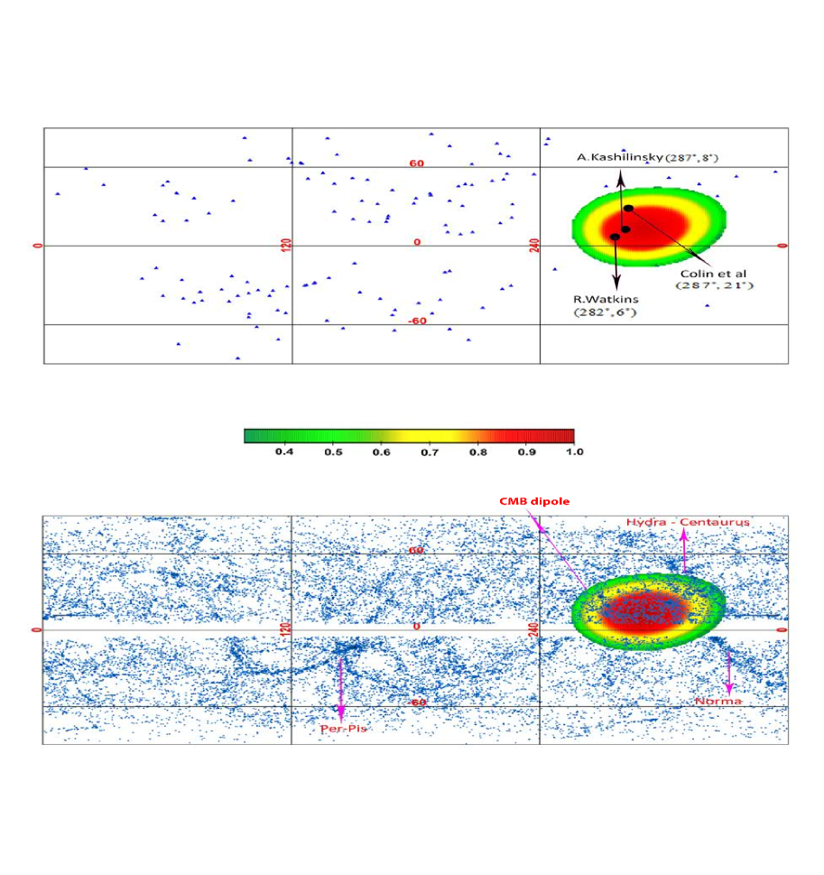
Figure 1: Top panel: Probability distribution function related to bulk flow direction, written on the rectangle in galactic coordinates and shown the results of some previous studies , in the redshift less than 0.035 using 200,000 data and low panel: area $(1-\sigma)$ is plotted for the bulk flow direction written on the rectangle in galactic coordinates for redshift less than 0.035. Also, the coordinates of important superclusters are shown in this redshift .

6 Redshift interval less than 0.06

In the redshift $0.015<z<0.06$, there are 174 supernovae. In Figure 2(top panel), the probability distribution function for the bulk current on a sphere in galactic coordinates is written. The simulation results with more than $2\times 10^{5}$ data show that the bulk current in this area is moving in the direction of $(l,b)=(300^{+15}_{-18},3^{+10}_{-11})$, which is close to the direction of the constellations Centaurus and Hydra. The Shapley supercluster is also located in the redshift and it is thought that all superclusters are moving towards this supercluster. This is consistent with the results of studies (Lavaux et al, 2010) ($(l,b)=(295^{+18}_{-18},14^{+18}_{-18})$)‌, (Kocevski et al, 2006) ($(l,b)=(306.44,29.71)$) , (Feldman et al, 2010) ($(l,b)=(282^{+11}_{-11},6^{+6}_{-6})$) (De et al, 2011) ($(l,b)=(290^{+39}_{-31},20^{+30}_{-30})$)‌‌ . Figure2 portrays the region $(1-\sigma)$ corresponding to the direction of the bulk flow on a rectangle in the galactic coordinates. Another noteworthy point that is inherent in Figure 2(low panel) is that the direction of motion of the local group galaxy is at the edge of the region’s confidence level $(1-\sigma)$ in the direction of the bulk current, which is indicative of the fact that the reconstruction of the direction of motion of the local cluster by Bulk flow for distances less than $150h^{-1}Mpc$ leads to better results.

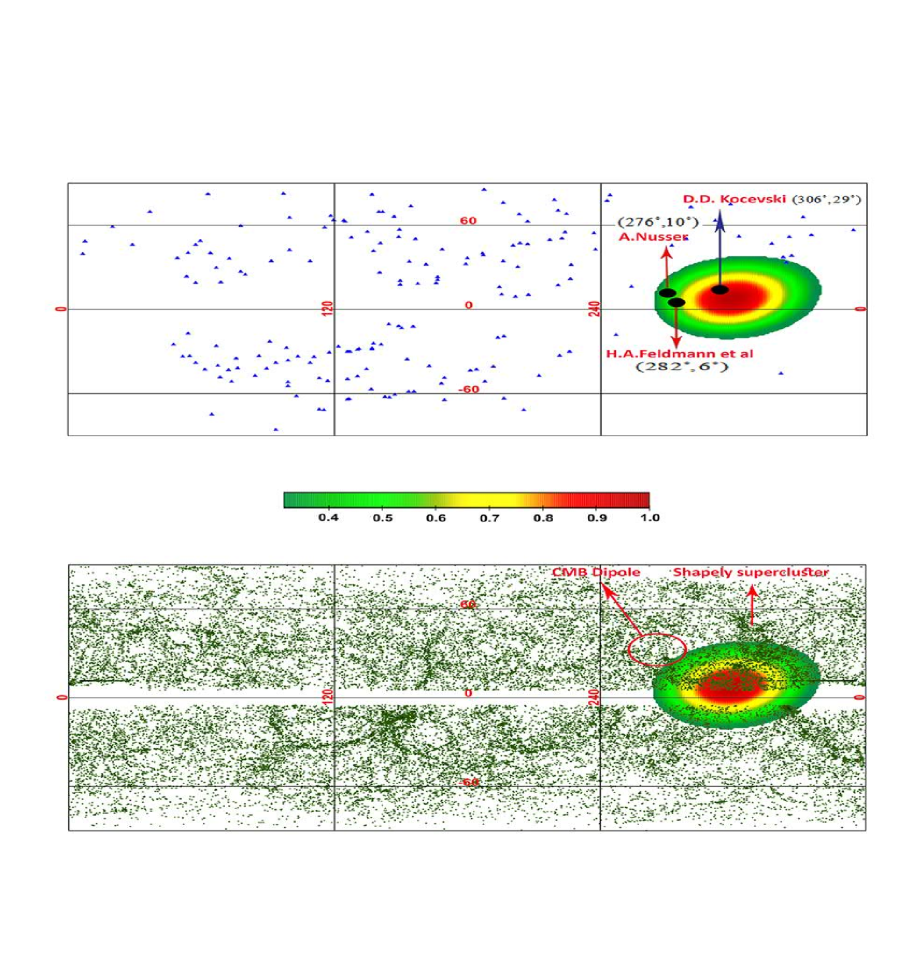
Figure 2: Top panel: Probability distribution function related to bulk flow direction, written on the rectangle in galactic coordinates and shown the results of some previous studies , in the redshift less than 0.06 using 200,000 data and low panel: area $(1-\sigma)$ is plotted for the bulk flow direction written on the rectangle in galactic coordinates for redshift less than 0.06. Also, the coordinates of important superclusters are shown in this redshift .

7 Redshift interval less than 0.1

In the redshift interval $0.015<z<0.1$, there are 211 supernovae. In this redshift, a value obtained for the bulk flow direction is $(l,b)=(302^{+10}_{-12},5^{+8}_{-9})$, which is consistent with the results of the (Watkins et al, 2009) ($(l,b)=(283^{+14}_{-18},12^{+14}_{-14})$)‌. Figures (3) demonstrate the results of this simulation. As shown in Figure 3(low panel), the direction of movement of the local cluster (CMB dipole) is outside the region $(1-\sigma)$ of the bulk current, which indicates that the farther we go from $150h^{-1}Mpc$, The difference between the direction of movement of the local cluster and the direction of the bulk flow increases. The results of many previous studies for different areas are given in Table (1).

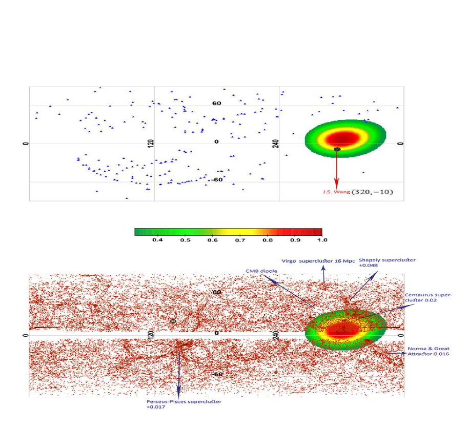
Figure 3: Top panel: Probability distribution function related to bulk flow direction, written on the rectangle in galactic coordinates and shown the results of some previous studies , in the redshift less than 0.1 using 200,000 data and low panel: area $(1-\sigma)$ is plotted for the bulk flow direction written on the rectangle in galactic coordinates for redshift less than 0.1. Also, the coordinates of important superclusters are shown in this redshift .

The other parameters that are fitted are the parameters of the Chameleon model $(\alpha,\beta)$, which is determined using the bulk flow model. In Figure 4, the probability distributions for these parameters are plotted for 60,000 data. As it is known, the range of these parameters is of the order of one, which some studies have predicted the same value.

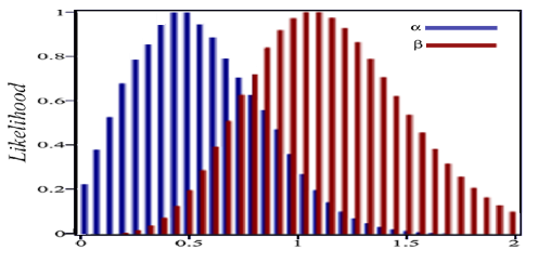
Figure 4: Probability distribution function related to Chameleon parameters $(\alpha,\beta)$ fitted to supernovae type Ia in the Bulk flow model.

Table 1: List of studies on bulk flow

$Ref$	$velocity$	$redshift$	$l^{o}$	$b^{o}$	$distance$
	$kms^{-1}$		$degree$	$degree$	$h^{-1}Mpc$
(k2 et al, 2010)	$1000$	$z\leq 0.03$	$287\pm 9$	$8\pm 6$	$300$
(Watkins et al, 2009)	$407\pm 81$	$z\leq 0.2$	$283\pm 14$	$12\pm 14$	$100$
(Kocevski et al, 2006)	$507$	$0.035\leq z\leq 0.055$	$306.44$	$29.71$	$105-165$
(Turnbull et al, 2012)	$249\pm 276$	$z\leq 0.2$	$319\pm 18$	$7\pm 14$	$100$
(Colin et al, 2011)	$250^{+190}_{-160}$	$0.045<z<0.06$	$287$	$21$	$90-240$
(Watkins et al, 2009)	$416\pm 78$	$z=0.0167$	$282$	$60$	$100$
(Lavaux et al, 2010)	$473\pm 128$	$0.035<z<0.055$	$220$	$25$	$100$
(Nusser & Davis, 2011)	$257\pm 44$	$0.035<z<0.055$	$276\pm 6$	$10\pm 6$	$100$
(Feldman et al, 2010)	$416\pm 78$	$0.015<z<0.06$	$282\pm 11$	$6\pm 6$	$100$

8 Comparison of bulk flow direction with dark energy dipole direction

One of the anisotropies observed by the analysis of observational data is the anisotropy of the dark energy distribution or the dipole of dark energy. Since one of the most likely causes of the universe’s accelerated expansion is dark energy, studies have suggested that dark energy is distributed as a dipole, which causes the anisotropic expansion of the universe and creates a preferred direction for cosmology(Antoniou & Perivolaropoulos, 2010)-(Yang et al, 2014). On the other hand, it seems that the direction of bulk flow on a large scale is close to the dipole of dark energy. As such to investigate this issue, we calculate the dipole of dark energy in the Chameleon model. Numerous studies have examined the dipole of dark energy in a variety of ways (Antoniou & Perivolaropoulos, 2010)-(Yang et al, 2014) here using equation (2-1) in reference (Antoniou & Perivolaropoulos, 2010) and equation (5-22) in reference (Salehi & Aftabi, 2016). We deal with dipoles (details and equations of dark energy in red transfer less than 0.1 (equivalent to approximately $300h^{-1}Mpc$ distance) are given in the references mentioned). In Figure 5, the probability distribution function in region $(1-\sigma)$ for the dipole direction of dark energy on a sphere in galactic coordinates is written and its direction is compared with the direction of the bulk current in the same region. As can be seen from the figure, these two regions overlap well, indicating a unifying convergence between the bulk flow direction and the direction of dark energy dipole at distances greater than $150h^{-1}Mpc$ with the direction (1 to 3); it can therefore be concluded that the bulk current converges in the transition to lower reds and at distances less than ($150h^{-1}Mpc$) local cluster motion.However as the distance increases, the degree of convergence decreases and the direction of the bulk current approaches the polarity of the dark energy.

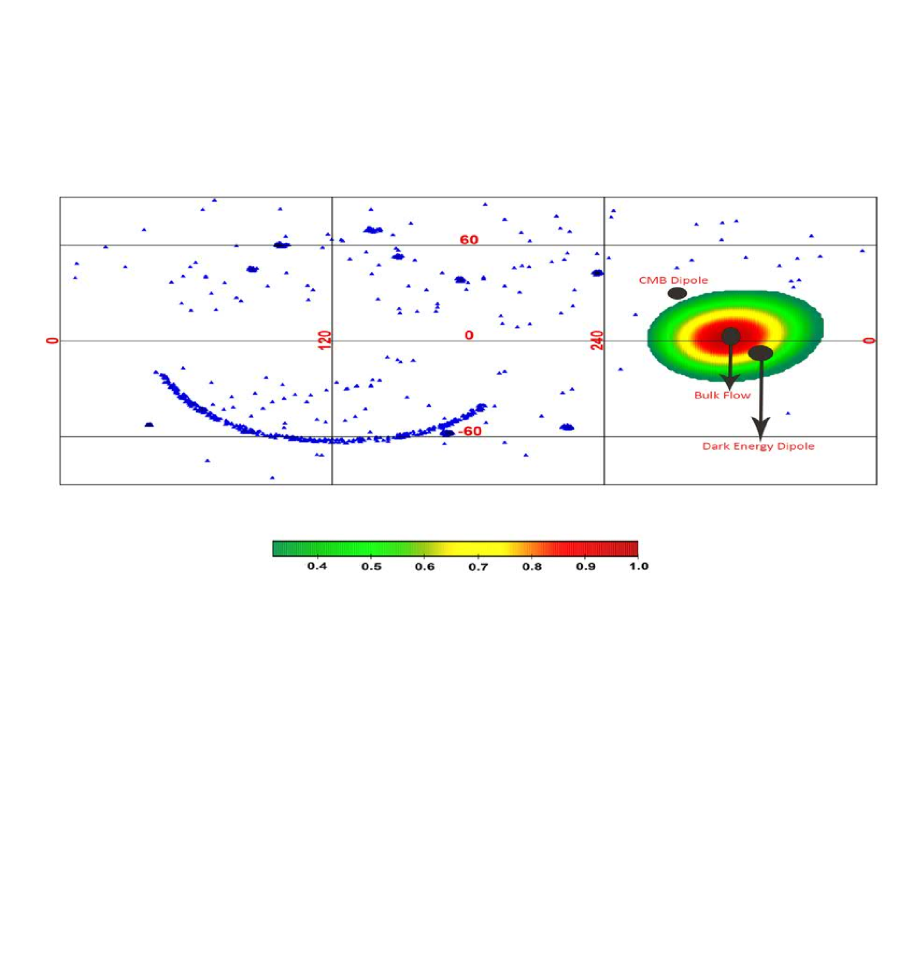
Figure 5: Comparison of bulk flow direction and direction of dark energy dipole in region $(1-\sigma)$.

9 Conclusion

In this paper, we have shown that Chameleon fields can be the source of dark energy dipole and cosmic background radiation dipole at the same time. On the other hand, the study of region $(1-\sigma)$, in the redshift less than 0.035, showed that not only are our results well consistent with studies that confirm the flow of the bulk, but also the direction of movement of galaxies of the local group in region $(1-\sigma)$ in the direction of bulk flow. These two are towards the Hydra-Centaurus supercluster, which is in the same redshift. Similarly, in the redshift, it is less than 0.06 (in the direction of movement of the local cluster in the region $(1-\sigma)$ in the direction of the bulk flow, and these two are in turn in the direction of the Shapley supercluster. Although the Chameleon model justifies the convergence between the direction of the bulk current and the motion of a local group galaxy with good accuracy $(1-\sigma)$ in the direction of high-density structures such as superclusters, this may not come as a surprise at short distances,a concept which is thought to be the source of all these mass distribution disparities. Despite this it is certainly interesting to study the convergence of the direction of the bulk current with other cosmic anisotropies that originate in the early evolution of the universe, and may be a response to the origin of the bulk current, the direction of motion of the local group galaxies, and the formation of large structures. One of these anisotropies observed by the analysis of observational data is dark energy distribution or dark energy dipole anisotropy. Considering that one of the most probable causes of the accelerated expansion of the universe is dark energy, studies confirm that dark energy is distributed as a bipolar, which causes the anisotropic expansion of the universe and creates a preferred direction for the universe to integrate. In this paper, the dipole direction of dark energy in Chameleon model is obtained in the direction of galactic coordinates $(l,b)=(324^{+18}_{-18},-4^{+12}_{-12})$, which is in good agreement with the direction of the bulk flow in the region $(1-\sigma)$. Therefore, these studies reveal that the Chameleon model can be a good option to justify anisotropy on both small and large scales. Given the properties of these fields, they may also be a good justification for fixed spatial anisotropies of fine structure constant(fixed fine structure constant dipole), which we intend to examine in future studies.

References

- Conklin (1969) Conklin, E.K. 1969, Nature, 222, 971
- Henry (1971) Henry, P.S. 1971, Nature, 231, 516
- Smoot et al (1977) Smoot, G. F., Gorenstein, M. V., & Muller, R. A. 1977, Phys. Rev. Lett., 39,898
- Villumsen & Strauss (1987) Villumsen, J., & Strauss, M. 1987, ApJ, 322, 37
- Shaya (1984) Shaya,E.1984,ApJ280,470
- Tammann & andSandage (1985) Tammann,G.andSandage,A.1985,ApJ294,81
- Aaronson et al (1986) Aaronson, M., Bothun, G., Mould, J., Huchra, J., Schommer, R., & Cornell, M. 1986, ApJ, 302, 536
- Dressier et al (1987) Dressier, A., Faber, S., Burstein, D., Davies, R., Lynden-Bell, D., Terlevich, R., & Wegner, G. 1987, ApJ, 313, L37
- Lynden-Bell et al (1988) Lynden-Bell,D.,Faber,S.M.,Burstein,D.,Davies,R.L.,Dressler,A.,Terlevich,R.J.andWegner,G.1988,ApJ326,19
- Bothun et al (1992) Bothun, G. D., Harris, H. C., & Hesser, J. E. 1992, PASP, 104, 1220
- Kogut et al (1993) A. Kogut et al., 1993, ApJ, 419, 1
- Hoffman et al (2001) Hoffman Y., Eldar A., Zaroubi S., Dekel A., 2001, preprint (astro-ph/ 0102190)
- Kocevski et al (2006) Kocevski, D. D. & Ebeling, H. 2006, ApJ, 645, 1043
- k et al (2008) A. Kashlinsky; F. Atrio-Barandela, D. Kocevski, and H. Ebeling, Astrophys. J. 686, L49 (2008).
- k1 et al (2009) Kashlinsky, A., Atrio-Barandela, F., Ko cevski, D., & Eb eling, H. 2009, ApJ, 691, 1479
- k2 et al (2010) A. Kashlinsky; F. Atrio-Barandela, H. Ebeling, A. Edge, and D. Kocevski, Astrophys. J. 712, L81 (2010).
- Atrio et al (2015) Atrio-Barandela, F.; Kashlinsky, A.; Ebeling, H.; Fixsen, D. J.; Kocevski, D. (2015. Astrophys. J. 810 (2):143.
- Colin et al (2011) Colin, J., Mohayaee, R., Sarkar, S., Shafieloo, A. 2011, MNRAS, 414, 264
- Dai et al (2011) Dai, D.-C., Kinney, W. H., & Sto jkovic, D. 2011, J. Cosmol. Astropart. Phys., JCAP04(2011)015
- Turnbull et al (2012) Turnbull, S. J., Hudson, M. J., Feldman, H. A., et al. 2012, MNRAS, 420, 447
- fien et al (2013) U. Feindt et.al 2013,arXiv:1310.4184v3
- Hudson et al (2004) Hudson, M. J., Smith, R. J., Lucey, J. R., & Branchini, E. 2004, MNRAS, 352,61
- Watkins et al (2009) Watkins, R., Feldman, H. A., & Hudson, M. J. 2009, MNRAS, 392, 743
- Lavaux et al (2010) Lavaux, G., Tully, R. B., Mohayaee, R., & Colombi, S. 2010, ApJ, 709, 483
- Nusser & Davis (2011) Nusser, A. & Davis, M. 2011, ApJ, 736, 93
- Branchini et al (2012) Branchini, E., Davis, M., & Nusser, A. 2012, MNRAS, 424, 472
- Ma & Scott (2017) Ma, Y.-Z. & Scott, D. 2013, MNRAS, 428, 2017
- Planck (2013) Planck Collaboration. 2013, ArXiv e-prints, arxiv:1303.5090
- Bon et al (2006) Camille Bonvin, Ruth Durrer, and Martin Kunz Phys. Rev. Lett. 96, 191302 – Published 17 May 2006
- Hui & Patrick (2006) Lam Hui and Patrick B. Greene, Phys.Rev.D73:123526,2006
- Khoury & Weltman (2004) J. Khoury and A. Weltman, astro-ph/0309300 and astro-ph/0309411,2004
- Ferreira & Joyce (1998) P. G. Ferreira and M. Joyce, Phys. Rev. Lett. 79, 4740(1997); Phys. Rev D 58, 023503 (1998).
- Wetterich (1988) C. Wetterich, Nucl. Phys. B302, 668 (1988).
- Farajollahi & Salehi (2012) H.Farajollahi, A. Salehi, Physical Review D 85, 083514 (2012)
- Farajollahi & Salehi (2010) Amanullah R. et al., 2010, ApJ, 716, 712.
- Feldman et al (2010) Feldman H. A., Watkins R., Hudson M. J., 2010, MNRAS, 407,2328
- De et al (2011) De-Chang Dai1, William H. Kinney2 and Dejan Stojkovic,arXiv: 1102.0800v2,2011
- Antoniou & Perivolaropoulos (2010) Antoniou I., Perivolaropoulos L., 2010, JCAP, 12, 12
- Cai et al (2013) R.-G. Cai, Y.-Z. Ma, B. Tang and Z.-L. Tuo, Phys. Rev. D 87, 123522 (2013).
- Mariano & Perivolaropoulos (2012) Mariano A., Perivolaropoulos L., 2012, Phys. Rev. D, 86, 083517
- Armendariz-Picon (2004) C. Armendariz-Picon, JCAP 0407, 007 (2004).
- Zhao & Zhang (2006) W. Zhao and Y. Zhang, Class. Quant. Grav. 23, 3405 (2006).
- Zhao & Zhang (2006) W. Zhao and Y. Zhang, Phys. Lett. B 640, 69 (2006).
- Zhao & Zhang (2007) Y. Zhang, T. Y. Xia, W. Zhao, Class. Quant. Grav. 24, 3309 (2007).
- Salehi & Aftabi (2016) A. Salehi and S. Aftabi, JHEP, 09(2016)140
- Salehi & Aftabi (2016) A. Salehi and S. Aftabi, Int. J. Mod. Phys. D 25, 1650042 (2016)
- Koivisto & Mota (2008) T. S. Koivisto and D. F. Mota, JCAP 0808, 021 (2008).
- Yang et al (2014) Yang X. F., Wang F. Y., Chu Z., 2014, MNRAS, 437, 1840