Optimal multilevel adaptive FEM for the Argyris element

Abstract

The main drawback for the application of the conforming Argyris FEM is the labourious implementation on the one hand and the low convergence rates on the other. If no appropriate adaptive meshes are utilised, only the convergence rate caused by corner singularities [Blum and Rannacher, 1980], far below the approximation order for smooth functions, can be achieved. The fine approximation with the Argyris FEM produces high-dimensional linear systems and for a long time an optimal preconditioned scheme was not available for unstructured grids. This paper presents numerical benchmarks to confirm that the adaptive multilevel solver for the hierarchical Argyris FEM from [Carstensen and Hu, 2021] is in fact highly efficient and of linear time complexity. Moreover, the very first display of optimal convergence rates in practically relevant benchmarks with corner singularities and general boundary conditions leads to the rehabilitation of the Argyris finite element from the computational perspective.

1 Introduction

This paper discusses numerical aspects of an adaptive multilevel algorithm based on the Argyris finite element for the biharmonic plate problem with inhomogeneous mixed boundary conditions.

1.1 Motivation

The conforming discretisation of fourth-order problems on unstructured domains with the finite element method (FEM) requires complicated $C^{1}$ elements like Hsieh-Clough-Tocher or Argyris elements [13]. Classical a priori analysis yields optimal rates of convergence for sufficiently smooth solutions only. In practical applications however, singularities in the data or boundary of the domain lead to singular solutions [1] and reduced convergence rates. This motivated the development of several alternative conforming schemes to reduce the computational overhead, e.g., the Bell element as an modification of the Argyris element with less degrees of freedom [13]. In contrast, the non-conforming adaptive Morley FEM is known to be optimal and comes with an implementation in only 30 lines of MATLAB [9].

Adaptive mesh-refinement techniques for the many $C^{1}$ conforming FEMs remained unclear from the theoretical perspective until the preceding work of Carstensen and Hu [11]. Their slight modification to the Argyris FEM comes with an adaptive algorithm and an efficient multilevel solver at the cost of a negligibly increased computational effort. They prove optimal convergence rates and optimality of the proposed multilevel solver based on a multigrid V-cycle for the so-called hierarchical Argyris FEM. Naturally, the comparison with the standard Argyris FEM is an important aspect from the practical viewpoint. This and numerical evidence of the optimality in physically relevant benchmarks justify a rehabilitation of the Argyris element for fourth-order problems. Since [11] exclusively discusses homogeneous boundary conditions, the application to meaningful models in solid mechanics requires the extension to general boundary conditions.

1.2 Plate problem and FEM model

This paper considers the biharmonic plate equation with inhomogeneous mixed boundary conditions as a model example of a fourth-order problem given by

$$\begin{aligned} \Delta^{2}u=F&&\text{in }\Omega,&&u=g&&\text{on }{\Gamma_{C}}\cup{\Gamma_{S}},&&{\partial_{\nu}u}={\partial_{\nu}g}&&\text{on }{\Gamma_{C}}.\end{aligned}$$ (1)

The function $u\in H^{2}(\Omega)$ describes the displacement of a thin structure or plate with mid-section $\Omega$ under the influence of a force $F$. Different boundary conditions model how the plate is hold in place, see the survey [26]. Clamped boundary conditions apply on ${\Gamma_{C}}\subset\overline{\Omega}$ and prescribe the displacement and bending of the plate in terms of the globally defined boundary data $g\in H^{2}(\Omega)$. On ${\Gamma_{S}}\subset\overline{\Omega}$, the plate is simply-supported and only its displacement is fixed. This paper extends the a posteriori analysis of [11] to general boundary conditions under reasonable assumptions. The first one is classical in the theory of plates [6] and requires the relatively open boundary components ${\Gamma_{C}},{\Gamma_{S}}\subset\overline{\Omega}$ of co-dimension one to ensure that the test space

$$V\coloneqq\{v\in H^{2}(\Omega)\ |\ v={\partial_{\nu}v}=0\text{ on }{\Gamma_{C}},v=0\text{ on }{\Gamma_{S}}\}$$

solely contains the trivial affine function, i.e., $V\cap P_{1}(\Omega)=\{0\}$. Thus, the weak Hessian $D^{2}$ defines the bilinear energy form $a(v,w)\coloneqq(D^{2}v,D^{2}w)_{L^{2}(\Omega)}$ for $v,w\in H^{2}(\Omega)$ that is positive definite on $V$ and induces the energy norm $|\!|\!|\bullet|\!|\!|\coloneqq a(\bullet,\bullet)^{1/2}$. The weak form of the plate problem (1) for given force $F\in V^{\prime}$ and boundary data $g\in H^{2}(\Omega)$ seeks the displacement $u\in g+V$ defined by

$$a(u,v) =F(v) \text{ for all }v\in V.$$ (2)

The standard (resp. hierarchical) Argyris FEM on a triangulation $\mathcal{T}$ seeks an approximation $u_{h}$ of $u$ in the standard (resp. extended) Argyris space $\mathfrak{A}(\mathcal{T})\subset P_{5}(\mathcal{T})\cap H^{2}(\Omega)$ of conforming piecewise quintic polynomials. This requires a discrete analogon of the boundary data $g$ and a natural choice comes from the nodal interpolation operator $\mathcal{I}:C^{2}(\overline{\Omega})\to\mathfrak{A}(\mathcal{T})$ if $g\in C^{2}(\overline{\Omega})$ is sufficiently smooth. The discrete approximation $u_{h}\in\mathcal{I}g+V(\mathcal{T})$ to (2) in the discrete test space $V(\mathcal{T})\coloneqq V\cap\mathfrak{A}(\mathcal{T})$ solves

$$a(u_{h},v_{h}) =F(v_{h}) \text{ for all }v_{h}\in V(\mathcal{T}).$$ (3)

The a posteriori analysis in this paper assumes that $F\in V^{\prime}$ is the sum of an $L^{2}$ contribution plus point forces. The main result establishes optimal convergence rates of the error $|\!|\!|u-u_{h}|\!|\!|$ and oscillations in an adaptive algorithm for slightly more regular boundary data $g\in B$ in the space

$$B\coloneqq\left\{v\in C^{2}(\overline{\Omega})\ \middle|\ \begin{array}[]{ll}\text{for all edges }\Gamma\text{ of }\partial\Omega,&v_{|\Gamma}\in H^{3}(\Gamma)\text{ and }({\partial_{\nu}v})_{|\Gamma}\in H^{2}(\Gamma)\end{array}\!\!\!\right\}.$$ (5)

Note that this only imposes conditions on $g_{|{\Gamma_{C}\cup\Gamma_{S}}}$ and ${\partial_{\nu}g}_{|{\Gamma_{C}}}$ (e.g., replace $g$ by any element from $g+V$).

1.3 Outline

Section 2 introduces some notation for the standard and hierarchical Argyris FEM for general boundary conditions and the adaptive algorithm. This paper is split into an analytical part preceding the numerical benchmarks in the second part. The a posteriori error analysis in section 3 extends the optimal rates of the hierarchical Argyris AFEM from [11] to mixed inhomogeneous boundary conditions. This directly leads to the equivalence of some computable a posteriori error estimator $\eta(\mathcal{T})$ to the exact error (up to oscillations) also for the standard Argyris FEM and motivates the comparison of the standard and hierarchical Argyris AEFM with the $\eta(\mathcal{T})$ driven adaptive algorithm in section 4. Section 5 discusses the application of multilevel-preconditioned iterative schemes for the solution of the discrete problem (3). A reliable and efficient estimator of the algebraic error provides numerical evidence for the interoperability of multigrid (MG) and preconditioned conjugated gradient (PCG) methods with the adaptive algorithm. Section 6 concludes with some remarks.

1.4 Overall notation

Standard notation for Lebesgue and Sobolev spaces and their norms applies throughout this paper. Let $H^{s}(K)$ abbreviate $H^{s}(\mathrm{int}(K))$ for closed $K\subset{\mathbb{R}}^{2}$. Consider an open bounded Lipschitz domain $\Omega\subset{\mathbb{R}}^{2}$. The polygonal boundary $\partial\Omega$ with vertices $\mathcal{V}_{\Omega}$ and edges $\mathcal{E}_{\Omega}$ decomposes into the relatively open, disjoint parts ${\Gamma_{C}},{\Gamma_{S}}$ and into $\partial\Omega\setminus({\Gamma_{C}\cup\Gamma_{S}})$. Let $P_{k}(K)$ denote the spaces of piecewise polynomials of total degree less than or equal $k\in{\mathbb{N}}_{0}$ on some triangle or edge $K\in\mathcal{T}\cup\mathcal{E}$ with diameter $h_{K}\in P_{0}(K)$. The associated $L^{2}$ projection reads $\Pi_{K,k}:L^{2}(K)\to P_{k}(K)$ and is defined by the $L^{2}$ orthogonality $(1-\Pi_{K,k})v\perp P_{k}(K)$ for all $v\in L^{2}(K)$. Let

$$P_{k}(\mathcal{T})\coloneqq\{p\in L^{\infty}(\Omega):p_{|T}\in P_{k}(T)\text{ for all }T\in T\}$$

denote the space of piecewise polynomials on a triangulation $\mathcal{T}$ of the domain $\Omega$. The partial derivatives $\partial_{v_{1},\dots,v_{j}}^{j}$ for the $j\in{\mathbb{N}}_{0}$ directions $v_{1},\dots,v_{j}\in{\mathbb{R}}^{2}$ define the functional $\partial_{v_{1},\dots,v_{j}}^{j}\delta_{z}:C^{j}(\overline{\Omega})\to{\mathbb{R}}$ by

$$\partial_{v_{1},\dots,v_{j}}^{j}\delta_{z}(f)\coloneqq(-1)^{j}\delta_{z}(\partial_{v_{1},\dots,v_{j}}^{j}f)=(-1)^{j}\partial_{v_{1},\dots,v_{j}}^{j}f(z) \text{ for all }f\in C^{j}(\overline{\Omega})$$

for the Dirac functional $\delta_{z}$ associated with some point $z\in\overline{\Omega}$.

2 Adaptive standard and hierarchical Argyris FEM

This section defines the adaptive standard Argyris FEM, e.g., [13], and the adaptive hierarchical Argyris FEM [11] for general boundary conditions.

2.1 Triangulation

Throughout this paper, $\mathcal{T}$ denotes a shape regular triangulation (in the sense of Ciarlet) of the polygonally bounded Lipschitz domain $\Omega\subset{\mathbb{R}}^{2}$ with vertices $\mathcal{V}$ and edges $\mathcal{E}$ resolving the boundary conditions, i.e., $\bigcup\mathcal{E}(\Gamma_{X})=\overline{\Gamma}_{X}$ for $\mathcal{E}(\Gamma_{X})\coloneqq\{E\in\mathcal{E}\ :\ E\subset\overline{\Gamma}_{X}\}$ and $\Gamma_{X}={\Gamma_{C}},{\Gamma_{S}}$. The set $\mathcal{E}(\Omega)$ (resp. $\mathcal{E}(\partial\Omega)$) denotes the interior (resp. exterior) edges and the same notation applies for the vertices $\mathcal{V}$, edge-midpoints $\mathcal{M}\coloneqq\{\mathrm{mid}\;E\ :\ E\in\mathcal{E}\}$, and nodes $\mathcal{N}\coloneqq\mathcal{V}\cup\mathcal{M}$. Given a triangle $T\in\mathcal{T}$, denote the unit outer normal vector on the edges $E\in\mathcal{E}(T)$ of $T$ by $\nu_{T}$. Associate every edge $E\in\mathcal{E}$ with a unit tangential $\tau_{E}$ and normal $\nu_{E}$ of fixed orientation. If the context allows, the index $E$ with partial derivatives in directions $\tau_{E},\nu_{E}$ is omitted. The jump $[q]_{E}\in L^{2}(E)$ of $q\in H^{1}(\mathcal{T})$ along an interior edge $E=T_{+}\cap T_{-}\in\mathcal{E}(\Omega)$ reads $[q]_{E}\coloneqq q_{|T_{+}}-q_{|T_{-}}$ and $[q]_{E}\coloneqq q$ for boundary edges $E\in\mathcal{E}(\partial\Omega)$.

Fix an initial triangulation $\mathcal{T}_{0}$ of $\Omega$ with vertices $\mathcal{V}_{0}$ and the set $\mathbb{T}(\mathcal{T}_{0})$ of all admissible refinements generated by the newest-vertex bisection (NVB) [25, 5] of $\mathcal{T}_{0}$. Note that the mesh-closure estimate requires no initial condition for $\mathcal{T}_{0}$ in two space dimensions [20, Thm. 2]. For simplicity, some constructions related to a triangulation $\mathcal{T}\in\mathbb{T}(\mathcal{T}_{0})$ are formulated in terms of some sequence $(\mathcal{T}_{0},\mathcal{T}_{1},\dots,\mathcal{T}_{L}=\mathcal{T})$ of successive NVB refinements. However, this construction will only depend on $\mathcal{T}_{0}$ and not on the chosen sequence.

2.2 Standard and extended Argyris space

The standard Argyris space on $\mathcal{T}$, associated to the quintic Argyris element, consists locally of quintic polynomials and reads

$$\mathfrak{A}_{\rm std}(\mathcal{T})\coloneqq\left\{v_{h}\in P_{5}(\mathcal{T})\cap C^{1}(\Omega):D^{2}v_{h}\text{ is continuous at every }z\in\mathcal{V}\right\}.$$ (6)

The extension to higher-order elements, e.g., the Argyris element of order seven is straightforward and not addressed in this paper. Notice that the continuity requirement of the Hessian at $z\in\mathcal{V}$ makes the standard Argyris space not hierarchical, i.e., in general $\mathfrak{A}_{\rm std}(\mathcal{T})\not\subseteq\mathfrak{A}_{\rm std}(\widehat{\mathcal{T}})$ for a refinement $\widehat{\mathcal{T}}$ of $\mathcal{T}$. In fact, the second-order normal-normal derivative $\partial_{\nu_{E}\nu_{E}}^{2}$ at some edge’s midpoint $z=\mathrm{mid}\;E$ could be discontinuous across an edge $E\in\mathcal{E}(\Omega)$ in $\mathfrak{A}_{\rm std}(\mathcal{T})$, whereas (6) enforces its continuity in $\mathfrak{A}_{\rm std}(\widehat{\mathcal{T}})$ for any refinement $\widehat{\mathcal{T}}$ of $\mathcal{T}$ that contains $z\in\widehat{\mathcal{V}}$. The extended Argyris space

$$\mathfrak{A}_{\rm ext}(\mathcal{T})\coloneqq\mathfrak{A}_{\rm std}(\mathcal{T}_{0})+\mathfrak{A}_{\rm std}(\mathcal{T}_{1})+\dots+\mathfrak{A}_{\rm std}(\mathcal{T}_{\ell})$$ (7)

is hierarchical and a minimal extension with respect to the sequence of successive refinements $\mathcal{T}_{0},\dots,\mathcal{T}_{\ell}=\mathcal{T}\in\mathbb{T}(\mathcal{T}_{0})$. The dependence on the initial triangulation is clear but the definition is in fact independent of the sequence in (7), see [11] for further details. Throughout this paper, let $\mathfrak{A}(\mathcal{T})$ denote either $\mathfrak{A}_{\rm std}(\mathcal{T})$ or $\mathfrak{A}_{\rm ext}(\mathcal{T})$ whenever no distinction is needed and define the (conforming) discrete test space

$$V(\mathcal{T})\coloneqq\{v_{h}\in\mathfrak{A}(\mathcal{T})\ :\ v_{h}=0\text{ on }{\Gamma_{C}\cup\Gamma_{S}}\text{ and }{\partial_{\nu}v}_{h}=0\text{ on }{\Gamma_{C}}\}=\mathfrak{A}(\mathcal{T})\cap V.$$ (8)

2.3 Local coordinate system

The correct resolution of the boundary data and the degrees of freedom for the hierarchical Argyris FEM require control of certain partial derivatives at the vertices. Fix two directions $\{\xi_{z},\zeta_{z}\}$ for each vertex $z\in\mathcal{V}$, spanning ${\mathbb{R}}^{2}$ (thought of as a local coordinate system), under the two following conditions. These are given in terms of some sequence $\mathcal{T}_{0},\dots,\mathcal{T}_{L}=\mathcal{T}$ of successive refinements of the initial triangulation $\mathcal{T}_{0}$ but only depend on $\mathbb{T}(\mathcal{T}_{0})$.

		$\omega=\pi$		$\omega\neq\pi$
$E_{0}$	$E_{1}$	$\{\xi_{z},\zeta_{z}\}$	$J(z)$	$\{\xi_{z},\zeta_{z}\}$	$J(z)$
${\Gamma_{C}}$	${\Gamma_{C}}$	$\{\tau_{0},\nu_{0}\}$	$\{1,2,3,4,5\}$	$\{\tau_{0},\nu_{0}\}$	$\{1,2,3,4,5,6\}$
${\Gamma_{C}}$	${\Gamma_{S}}$	$\{\tau_{0},\nu_{0}\}$	$\{1,2,3,4,5\}$	$\{\tau_{0},\nu_{0}\}$	$\{1,2,3,4,5\}$
${\Gamma_{C}}$	${\Gamma_{F}}$	$\{\tau_{0},\nu_{0}\}$	$\{1,2,3,4,5\}$	$\{\tau_{0},\nu_{0}\}$	$\{1,2,3,4,5\}$
${\Gamma_{S}}$	${\Gamma_{S}}$	$\{\tau_{0},\nu_{0}\}$	$\{1,2,4\}$	$\{\tau_{0},\tau_{1}\}$	$\{1,2,3,4,6\}$
${\Gamma_{S}}$	${\Gamma_{F}}$	$\{\tau_{0},\nu_{0}\}$	$\{1,2,4\}$	$\{\tau_{0},\nu_{0}\}$	$\{1,2,4\}$
${\Gamma_{F}}$	${\Gamma_{F}}$	any	$\emptyset$	any	$\emptyset$

Table 1: Local coordinate system $\{\xi_{z},\zeta_{z}\}$ at $z\in\mathcal{V}(\partial\Omega)$. Here, $\tau_{i}$ (resp. $\nu_{i}$) denotes the unit tangential (resp. normal) of $E_{i}\in\mathcal{E}(\partial\Omega),i=0,1$ with $z=E_{0}\cap E_{1}$ and $\omega$ the angle between $E_{0},E_{1}$

Condition 1: If $z\in\mathcal{V}(\Omega)\setminus\mathcal{V}_{0}$ is a new interior vertex, then the NVB-algorithm yields $z=\mathrm{mid}\;E$ for an edge $E$ of some previous triangulation $\mathcal{T}_{\ell},0\leq\ell\leq L-1$. In this case, set $\xi_{z}=\tau_{E}$ and $\zeta_{z}=\nu_{E}$.
Condition 2: For a boundary vertex $z\in\mathcal{V}(\partial\Omega)$, table 1 provides a choice that depends on the boundary conditions at the two boundary edges $E_{0},E_{1}\in\mathcal{E}(\partial\Omega)$ that meet at $z=E_{0}\cap E_{1}$.
No restrictions apply for the remaining cases where $z\in\mathcal{V}_{0}(\Omega)$ and the standard basis of ${\mathbb{R}}^{2}$ is a natural choice.

2.4 Degrees of freedom and nodal basis

There is $m(z)\coloneqq 1$ degree of freedom (dof) $L_{z,1}\coloneqq\partial_{\nu_{E}}\delta_{z}$ associated to each edge midpoint $z\in\mathcal{M}$. This is the evaluation in the normal direction $\nu_{E}$ to the edge $E\in\mathcal{E}$ at $\mathrm{mid}\;E=z$. The other $m(z)\coloneqq 6$ (resp. $m(z)\in\{6,7\}$) dofs for the standard (resp. extended) Argyris space are associated with the vertices $z\in\mathcal{V}$ and consist of partial derivatives in the local coordinate system $\{\xi_{z},\zeta_{z}\}$. For the standard Argyris space, they read

$$\delta_{z},\;\partial_{\xi_{z}}\delta_{z},\;\partial_{\zeta_{z}}\delta_{z},\;\partial_{\xi_{z}\xi_{z}}^{2}\delta_{z},\;\partial_{\xi_{z}\zeta_{z}}^{2}\delta_{z},\;\partial_{\zeta_{z}\zeta_{z}}^{2}\delta_{z} \text{ for }z\in\mathcal{V}$$

and for the extended Argyris space

$$\delta_{z},\;\partial_{\xi_{z}}\delta_{z},\;\partial_{\zeta_{z}}\delta_{z},\;\partial_{\xi_{z}\xi_{z}}^{2}\delta_{z},\;\partial_{\xi_{z}\zeta_{z}}^{2}\delta_{z},\;\partial_{\zeta_{z}\zeta_{z}}^{2}\delta_{z} \text{ for }z\in\mathcal{V}(\partial\Omega)\cup\mathcal{V}_{0},$$

$$\delta_{z},\;\partial_{\xi_{z}}\delta_{z},\;\partial_{\zeta_{z}}\delta_{z},\;\partial_{\xi_{z}\xi_{z}}^{2}\delta_{z},\;\partial_{\xi_{z}\zeta_{z}}^{2}\delta_{z},\;\partial_{\zeta_{z}\zeta_{z}}^{2}\delta_{z}^{+},\;\partial_{\zeta_{z}\zeta_{z}}^{2}\delta_{z}^{-} \text{ for }z\in\mathcal{V}(\Omega)\setminus\mathcal{V}_{0}.$$

They are enumerated in this order as $L_{z,1},...,L_{z,m(z)}$. Recall $\zeta_{z}=\nu_{E}$ for every new vertex $z\in\mathcal{V}(\Omega)\setminus\mathcal{V}_{0}$ where $z=\mathrm{mid}\;E$ for some historical edge $E$. The modification for the extended Argyris space is a split of the normal-normal derivative evaluation $\partial_{\zeta_{z}\zeta_{z}}^{2}\delta_{z}$($=\partial_{\nu_{E}\nu_{E}}^{2}\delta_{z}$) at these vertices into the one-sided evaluations

$$\partial_{\zeta_{z}\zeta_{z}}^{2}\delta_{z}^{\pm}\equiv\partial_{\nu_{E}\nu_{E}}^{2}\delta_{z}^{\pm}\coloneqq\lim_{x\in H_{\pm}(z)\to z}\partial_{\nu_{E}\nu_{E}}^{2}\delta_{x}$$ (9)

in the half-planes $H_{\pm}(z)\coloneqq\{x\in{\mathbb{R}}^{2}:\pm(x-z)\cdot\nu_{E}\geq 0\}$. This allows $\partial_{\nu_{E}\nu_{E}}^{2}v_{h}(z)$ to attain distinct values in $H_{+}(z)$ and $H_{-}(z)$ for $v_{h}\in\mathfrak{A}_{\rm ext}(\mathcal{T})$ at any such vertex $z\in\mathcal{V}(\Omega)\setminus\mathcal{V}$. Indeed, this modification is enough to obtain hierarchical spaces and shows independence of the chosen sequence in the definition of (7), see [11] for further details. Recall the set of nodes $\mathcal{N}\coloneqq\mathcal{V}\cup\mathcal{M}$ and denote the unique nodal basis (dual to the dofs) of $\mathfrak{A}(\mathcal{T})$ by $\mathcal{B}\coloneqq\{\varphi_{z,j}\ :\ z\in\mathcal{N},j=1,\dots,m(z)\}$. The choice of the local coordinates with $J(z)$ from table 1 for boundary vertices $z\in\mathcal{V}(\partial\Omega)$ ensures that

$$\{\varphi_{z,j}\in\mathcal{B}\ :\ j\not\in J(z)\text{ for }z\in\mathcal{V}(\partial\Omega)\text{ or }z\not\in\mathcal{M}({\Gamma_{C}})\}\subset\mathcal{B}$$ (10)

is a basis of the discrete test space $V(\mathcal{T})$ from (8) as the following result shows.

Proposition 2.1.

With $J(z)$ for $z\in\mathcal{V}(\partial\Omega)$ from table 1, it holds that

$$V(\mathcal{T})=\left\{v_{h}\in\mathfrak{A}(\mathcal{T})\ :\ \begin{aligned} L_{z,j}(v_{h})&=0\text{ for all }z\in\mathcal{V}(\partial\Omega),j\in J(z)\text{ and}\\ L_{z,1}(v_{h})&=0\text{ for all }z\in\mathcal{M}({\Gamma_{C}})\end{aligned}\right\}.$$

Proof.

Let $E=\mathrm{conv}\{P_{0},P_{1}\}\in\mathcal{E}(\partial\Omega)$ denote some boundary edge with normal $\nu\coloneqq\nu_{E}$ and tangential $\tau\coloneqq\tau_{E}$ and consider any $v_{h}\in\mathfrak{A}(\mathcal{T})$. It is well known, e.g., [13], that $v_{h|E}\equiv 0$ vanishes if and only if the nodal value of $v_{h}$ and its first two tangential derivatives along $E$ vanish at both endpoints $P_{0}$ and $P_{1}$, i.e.,

$$\delta_{z}(v_{h})=\partial_{\tau}\delta_{z}(v_{h})=\partial_{\tau\tau}^{2}\delta_{z}(v_{h})=0\quad\text{for }z=P_{0},P_{1}.$$ (11)

Similarly $({\partial_{\nu}v}_{h})_{|E}\equiv 0$ holds if and only if

$${\partial_{\nu}\delta}_{z}(v_{h})=\partial_{\tau\nu}^{2}\delta_{z}(v_{h})=0\quad\text{for }z=P_{0},P_{1}\quad\text{and}\quad{\partial_{\nu}\delta}_{\mathrm{mid}\;E}(v_{h})=0.$$ (12)

With $J(z)$ and $\{\xi_{z},\zeta_{z}\}$ from table 1, the conditions (11)–(12) translate into equivalent assertions in terms of the dofs. This shows the asserted identity. ∎

Notice the special treatment of a corner $z\in\mathcal{V}_{\Omega}$ of the domain $\Omega$ between edges $E_{0},E_{1}\in\mathcal{E}({\Gamma_{S}})$ in table 1 where the mixed derivative $\partial_{\tau_{0}\tau_{1}}^{2}$ remains a degree of freedom in $V(\mathcal{T})$.

2.5 Interpolation of boundary data

The duality relation between the dofs and the nodal basis defines the nodal interpolation operator $\mathcal{I}:C^{2}(\overline{\Omega})\to\mathfrak{A}(\mathcal{T}),$

$$\mathcal{I}v\coloneqq\sum_{z\in\mathcal{N}}\sum^{m(z)}_{j=1}L_{z,j}(v)\varphi_{z,j} \text{ for all }v\in C^{2}(\overline{\Omega}).$$ (13)

The following best-approximation property motivates the choice $\mathcal{I}g\in\mathfrak{A}(\mathcal{T})$ for the discrete boundary data $g\in B$ in the space of admissible boundary data $B$ from (5).

Lemma 2.2 (edge best-approximation).

Consider $v\in C^{2}(\overline{\Omega})$ and set $c_{\rm b}\coloneqq(1-45\pi^{-4})^{-1/2}$. If $v_{|E}\in H^{3}(E)$ and ${\partial_{\nu}v}_{|E}\in H^{2}(E)$ for some edge $E\in\mathcal{E}$, then

$$(a) \left\|\partial_{\tau\tau\tau}^{3}(1-\mathcal{I})v\right\|_{{L^{2}(E)}}=\phantom{c_{\rm b}}\left\|(1-\Pi_{E,2})\partial_{\tau\tau\tau}^{3}v\right\|_{{L^{2}(E)}},$$

$$(b) \left\|\partial_{\tau\tau\nu}^{3}(1-\mathcal{I})v\right\|_{{L^{2}(E)}}\leq c_{\rm b}\left\|(1-\Pi_{E,2})\partial_{\tau\tau\nu}^{3}v\right\|_{{L^{2}(E)}}.$$

Proof.

$(a)$ Repeated integration by parts and the exactness of the interpolation $\mathcal{I}$ at the vertices show $\partial_{\tau\tau\tau}^{3}\mathcal{I}v=\Pi_{E,2}\partial_{\tau\tau\tau}^{3}v$. Indeed, for arbitrary $p_{2}\in P_{2}(E)$, $\partial_{\tau\tau\tau}^{3}p_{2}\equiv 0$ verifies

$$\langle p_{2},\partial_{\tau\tau\tau}^{3}(1-\mathcal{I})v\rangle_{{L^{2}(E)}} =\langle\partial_{\tau\tau\tau}^{3}p_{2},(1-\mathcal{I})v\rangle_{{L^{2}(E)}}=0.$$

$(b)$ Let $b_{E}\in P_{2}(E)$ denote the edge-bubble function on $E=\mathrm{conv}\{P_{0},P_{1}\}$ that vanishes at both endpoints and attains $1=b_{E}(\mathrm{mid}\;E)$ at the midpoint. Consider an arbitrary $p_{2}\in P_{2}(E)$ and set $d_{E}\coloneqq{\Pi_{E,0}(\partial_{\nu}(1-\mathcal{I})v)}/(\Pi_{E,0}b_{E}^{2})\in{\mathbb{R}}$. Since ${\partial_{\nu}(}1-\mathcal{I})v$ and $b_{E}^{2}$ vanish to first order at the endpoints $P_{0}$ and $P_{1}$,

$$\langle p_{2},\partial_{\tau\tau\nu}^{3}(1-\mathcal{I})v-d_{E}\partial_{\tau\tau}^{2}b_{E}^{2}\rangle_{{L^{2}(E)}} =\langle\partial_{\tau\tau}^{2}p_{2},\Pi_{E,0}\left(\partial_{\nu}(1-\mathcal{I})v-d_{E}b_{E}^{2}\right)\rangle_{{L^{2}(E)}}=0$$

holds by the integration by parts formula and $d_{E}\partial_{\tau\tau}^{2}b_{E}^{2}=\Pi_{E,2}\partial_{\tau\tau\nu}^{3}v-\partial_{\tau\tau\nu}^{3}\mathcal{I}v\in P_{2}(E)$ follows. A direct computation reveals $\Pi_{E,0}b_{E}^{2}=8/15$ and $\partial_{\tau\tau\tau\tau}^{4}b_{E}^{2}=384|E|^{-4}$. This, integrating by parts twice, and the stability of the $L^{2}$ projection show

$$\begin{split}\left\|\Pi_{E,2}\partial_{\tau\tau\nu}^{3}v-\partial_{\tau\tau\nu}^{3}\mathcal{I}v\right\|_{{L^{2}(E)}}^{2}&=\langle d_{E}\partial_{\tau\tau\tau\tau}^{4}b_{E}^{2},\partial_{\nu}(1-\mathcal{I})v\rangle_{{L^{2}(E)}}\leq 720|E|^{-4}\left\|\partial_{\nu}(1-\mathcal{I})v\right\|_{{L^{2}(E)}}^{2}.\end{split}$$

By definition of the interpolation $\mathcal{I}$, $\partial_{\nu}(1-\mathcal{I})v$ vanishes at both endpoints and at $\mathrm{mid}\;E$. A split of the domain of integration $E$ into $E_{j}\coloneqq\mathrm{conv}\{P_{j},\mathrm{mid}\;E\},j=0,1$ allows the application of a Friedrichs inequality followed by a Poincaré inequality [22] with known constant $|E_{j}|/\pi$ on $E_{j},j=0,1$ separately. This, $|E_{0}|=|E_{1}|=|E|/2$, and the previous estimate show $\|\Pi_{E,2}\partial_{\tau\tau\nu}^{3}v-\partial_{\tau\tau\nu}^{3}\mathcal{I}v\|_{{L^{2}(E)}}^{2}\leq 45\pi^{-4}\|\partial_{\tau\tau\nu}^{3}(1-\mathcal{I})v\|_{{L^{2}(E)}}^{2}$. This and the Pythagoras Theorem prove

$$\left\|\partial_{\tau\tau\nu}^{3}(1-\mathcal{I})v\right\|_{{L^{2}(E)}}^{2} \leq\left\|(1-\Pi_{E,2})\partial_{\tau\tau\nu}^{3}v\right\|_{{L^{2}(E)}}^{2}+45\pi^{-4}\left\|\partial_{\tau\tau\nu}^{3}(1-\mathcal{I})v\right\|_{{L^{2}(E)}}^{2}.$$

Since $45\pi^{-4}<1$, an absorption of the rightmost term on the left-hand side concludes the proof. ∎

Consequently, the distance of the interpolation error $(1-\mathcal{I})g$ of $g\in B$ to the test space $V$ is bounded by boundary oscillations $\mathrm{osc}(\mathcal{S},g)$ defined on a subset of edges $\mathcal{S}\subseteq\mathcal{E}$ by

$$\mathrm{osc}^{2}(\mathcal{S},g) \coloneqq\sum_{E\in\mathcal{E}({\Gamma_{C}})\cap\mathcal{S}}|E|^{3}\|(1-\Pi_{E,2})\partial_{\tau\tau\nu}^{3}g\|_{L^{2}(E)}^{2}+\sum_{E\in\mathcal{E}({\Gamma_{C}\cup\Gamma_{S}})\cap\mathcal{S}}|E|^{3}\|(1-\Pi_{E,2})\partial_{\tau\tau\tau}^{3}g\|_{L^{2}(E)}^{2}.$$

Lemma 2.3.

There exists a constant $C_{\rm osc}>0$ solely depending on $\Omega$ such that for any $v\in B$,

$$\min_{w\in(1-\mathcal{I})v+{V}}|\!|\!|w|\!|\!|^{2}\leq C_{\rm osc}^{2}\mathrm{osc}^{2}(\mathcal{E}(\partial\Omega),v).$$

Proof.

It is straight-forward to verify that $t=(\varphi,\psi)\in\prod_{\Gamma\in\mathcal{E}_{\Omega}}(H^{3/2}(\Gamma)\times H^{1/2}(\Gamma))$, defined on each edge $\Gamma\in\mathcal{E}_{\Omega}$ of the polygonal domain $\Omega$ by

$$\varphi_{|\Gamma}=\begin{cases}{}(1-\mathcal{I})v&\text{ on }({\Gamma_{C}\cup\Gamma_{S}})\cap\Gamma,\\ 0&\text{ else}\end{cases}\quad\text{ and }\quad\psi_{|\Gamma}=\begin{cases}{}\partial_{\nu}((1-\mathcal{I})v)&\text{ on }{\Gamma_{C}}\cap\Gamma,\\ 0&\text{ else,}\end{cases}$$

belongs to the domain of the continuous right inverse of the trace map $\gamma_{1}:H^{2}(\Omega)\to\prod_{\Gamma\in\mathcal{E}_{\Omega}}(H^{3/2}(\Gamma)\times H^{1/2}(\Gamma))$ from [19]. The extension $\widehat{t}\in H^{2}(\Omega)$ of $t$ to the whole domain lies in $(1-\mathcal{I})v+V$ and the boundedness of the right-inverse verifies

$$\min_{w\in(1-\mathcal{I})v+{V}}|\!|\!|w|\!|\!|^{2}\leq\|\widehat{t}\|_{H^{2}(\Omega)}^{2}\lesssim\sum_{\Gamma\in\mathcal{E}_{\Omega}}\big{(}\left\|\varphi\right\|_{H^{3/2}(\Gamma)}^{2}+\left\|\psi\right\|_{H^{1/2}(\Gamma)}^{2}\big{)}.$$

Since $\varphi$ (resp. $\psi$) vanishes up to second (resp. first) order at the vertices of an exterior edge $E\in\mathcal{E}(\partial\Omega)$, the Gagliardo-Nierenberg inequality [7, Thm. 1] in combination with repeated Friedrichs inequalities shows

$$\min_{w\in(1-\mathcal{I})v+{V}}|\!|\!|w|\!|\!|^{2}\lesssim\sum_{E\in\mathcal{E}({\Gamma_{C}\cup\Gamma_{S}})}|E|^{3}\left\|\partial_{\tau\tau\tau}^{3}\varphi\right\|_{L^{2}(E)}^{2}+\sum_{E\in\mathcal{E}({\Gamma_{C}})}|E|^{3}\left\|\partial_{\tau\tau}^{2}\psi\right\|_{L^{2}(E)}^{2}.$$

The application of lemma 2.2 concludes the proof. ∎

2.6 Adaptive algorithm

Let the source $F\in V^{\prime}$ be given by an $L^{2}$ contribution $f\in L^{2}(\Omega)$ and point forces. Assume that the initial mesh is compatible with the point forces in the sense that their support is a vertex of the initial triangulation $z\in\mathcal{V}_{0}$, i.e., there are $\beta_{z}\in{\mathbb{R}}$ such that

$$F(v) \coloneqq(f,v)_{L^{2}(\Omega)}+\sum_{z\in\mathcal{V}_{0}}\beta_{z}v(z) \text{ for all }v\in V.$$ (14)

Given $T\in\mathcal{T}$ and the discrete solution $u_{h}\in\mathfrak{A}(\mathcal{T})$ to (3), the refinement indicator reads

$$\eta^{2}(\mathcal{T},T) =|T|^{2}\|f-\Delta^{2}u_{h}\|_{{L^{2}(\Omega)}}^{2}+\mathrm{osc}^{2}(\mathcal{E}(T),g)$$ (15)

$$+\sum_{E\in\mathcal{E}(T)\setminus\mathcal{E}({\Gamma_{C}})}|T|^{1/2}\|[\partial_{\nu\nu}^{2}u_{h}]_{E}\|_{{L^{2}(E)}}^{2}+\sum_{E\in\mathcal{E}(T)\setminus\mathcal{E}({\Gamma_{C}\cup\Gamma_{S}})}|T|^{3/2}\|[\partial_{\tau\tau\nu}^{3}u_{h}+\partial_{\nu}\Delta u_{h}]_{E}\|_{{L^{2}(E)}}^{2}$$

and drives the adaptive AFEM algorithm 1 for the standard and hierarchical Argyris FEM.

Algorithm 1 $\mathfrak{A}$-AFEM

Input: Initial triangulation $\mathcal{T}_{0}$, bulk parameter $0<\theta<1$

Solve the discrete problem (3) on $\mathcal{T}_{\ell}$ for $u_{\ell}\in\mathfrak{A}(\mathcal{T}_{\ell})$

Compute for all $T\in\mathcal{T}_{\ell}$ the local estimations $\eta(\mathcal{T}_{\ell},T)$ from (15)

Mark minimal subset $\mathcal{S}_{\ell}\subset\mathcal{T}_{\ell}$ with

$$\theta\sum_{T\in\mathcal{T}_{\ell}}\eta^{2}(\mathcal{T}_{\ell},T)\leq\sum_{T\in\mathcal{S}_{\ell}}\eta^{2}(\mathcal{T}_{\ell},T)$$

Refine $\mathcal{T}_{\ell}\longrightarrow\mathcal{T}_{\ell+1}$ as smallest NVB refinement of $\mathcal{T}_{\ell}$ with $\mathcal{S}_{\ell}\subseteq\mathcal{T}_{\ell}\setminus\mathcal{T}_{\ell+1}$

Output: Sequence of triangulations $\mathcal{T}_{\ell}$ and discrete solutions $u_{\ell}$

3 A posteriori analysis and optimality

This section proves the optimality of the adaptive hierarchical Argyris FEM ($\mathfrak{A}_{\rm ext}$-AFEM) for possibly inhomogeneous boundary data $g\in B$ and source terms of the form (14) including point forces. It follows that the error estimator $\eta(\mathcal{T})\coloneqq(\sum_{T\in\mathcal{T}}\eta^{2}(\mathcal{T},T))^{1/2}$ is reliable and efficient up to the oscillations $\mathrm{osc}(\mathcal{E}(\partial\Omega),g)$ and $\mathrm{osc}(\mathcal{T},f)\coloneqq\sum_{T\in\mathcal{T}}\|h_{T}^{2}(1-\Pi_{T,0})f\|_{L^{2}(T)}$. The axioms of adaptivity require the set $\mathbb{T}(N)\coloneqq\{\mathcal{T}\in\mathbb{T}(\mathcal{T}_{0})\ :\ |\mathcal{T}|-|\mathcal{T}_{0}|\leq N\}$ for $N\in{\mathbb{N}}$ and lead to the generalisation of [11, Thm. 6] following [18].

Theorem 3.1 (rate optimality of AFEM).

There exists $0<\Theta<1$ and for all $0<s<\infty$ some constant $\Lambda_{eq}>0$, only depending on $\mathbb{T}(\mathcal{T}_{0})$, on $\Theta$ and on $s$, such that the sequence of triangulations $(\mathcal{T}_{\ell})_{\ell}$ and discrete solutions $(u_{\ell})_{\ell}$ from the $\mathfrak{A}_{\rm ext}$-AFEM algorithm with $\theta\leq\Theta$ satisfies

$$\sup_{\ell\in{\mathbb{N}}_{0}} (1+|\mathcal{T}_{\ell}|-|\mathcal{T}_{0}|)^{s}\left(|\!|\!|u-u_{\ell}|\!|\!|+\mathrm{osc}(\mathcal{T}_{\ell},f)+\mathrm{osc}(\mathcal{E}_{\ell}(\partial\Omega),g)\right)$$

$$\leq\Lambda_{\rm eq}\sup_{N\in{\mathbb{N}}_{0}}(1+N)^{s}\min_{\mathcal{T}\in\mathbb{T}(N)}\left(|\!|\!|u-u_{h}|\!|\!|+\mathrm{osc}(\mathcal{T},f)+\mathrm{osc}(\mathcal{E}(\partial\Omega),g)\right).$$

The proof employs the axioms of adaptivity [5, 8, 12] and departs with a quasi-interpolation operator defined on $H^{2}(\Omega)$ in the spirit of [11] that interpolates exactly at the vertices. Let $\omega(T)\coloneqq\mathrm{int}(\bigcup\{K\in\mathcal{T}\ :\ T\cap K\neq 0\})$ denote the layer-1 patch around $T\in\mathcal{T}$ and $\gamma_{1}(v)\coloneqq(v_{|\partial\Omega},{\partial_{\nu}v}_{|\partial\Omega})$ the trace map on $H^{2}(\Omega)$ from [19].

Theorem 3.2 (discrete quasi-interpolation).

There are constants $c_{\rm apx},c_{\rm c}>0$ exclusively depending on $\mathbb{T}(\mathcal{T}_{0})$ such that for any admissible refinement $\widehat{\mathcal{T}}$ of $\mathcal{T}\in\mathbb{T}(\mathcal{T}_{0})$ there exists a linear operator $J:H^{2}(\Omega)\to\mathfrak{A}(\mathcal{T})$ satisfying, for any $v\in{H^{2}(\Omega)}$ and $\widehat{v}_{h}\in\mathfrak{A}(\widehat{\mathcal{T}})$,

1. $J(V)={V}(\mathcal{T})$ and $Jv(z)=v(z)$ for all $z\in\mathcal{V}$.

2. $\widehat{v}_{h}{}_{|T}=(J\widehat{v}_{h})_{|T}$ for any $T\in\mathcal{T}\cap\widehat{\mathcal{T}}$.

3. If $\gamma_{1}(v)\in\gamma_{1}(\mathfrak{A}(\mathcal{T}))$ then $\gamma_{1}(v)=\gamma_{1}(Jv)$ (preservation of discrete boundary data).

4. $|Jv|_{H^{m}(\Omega)}\leq c_{\rm c}|v|_{H^{m}(\Omega)}$ for $m=0,1,2$ (stability).

5. $\sum^{2}_{m=0}h_{T}^{m-2}|(1-J)v|_{H^{m}(T)}\leq c_{\rm apx}|v|_{H^{2}(\omega(T))}$ for any $v\in V$ (approximation property).

Proof.

Given any $v\in{H^{2}(\Omega)}$ and the nodal basis $\mathcal{B}$ from subsection 2.4 and follow the lines of [11, Thm. 2]. Define

$$Jv=\sum_{z\in\mathcal{N}}\sum^{m(z)}_{j=1}M_{z,j}(v)\varphi_{z,j}\in\mathfrak{A}(\mathcal{T})$$

as the discrete function with coefficients $M_{z,j}(v)$. The choice $M_{z,1}\coloneqq L_{z,1}=\delta_{z}$ ensures exact interpolation at the vertices $z\in\mathcal{V}$. The other functionals $M_{z,j}$ are chosen as in [11] for interior nodes and as in [17, Sec. 6] for the extension to the boundary such that $(b)$–$(c)$ hold. See [17, Sec. 7] for the stability $(d)$ and the approximation property $(e)$; further details can also be found in [18, Sec. 5] and are omitted here. ∎

This allows a discrete version of lemma 2.3. Set $C_{\rm osc,d}\coloneqq(1+c_{\rm b})c_{\rm c}C_{\rm osc}$ for the constants $c_{\rm b},C_{\rm osc},c_{\rm c}$ from lemmas 2.2, 2.3, and theorem 3.2, respectively.

Corollary 3.3.

Let $\widehat{\mathcal{T}}$ be an admissible refinement of $\mathcal{T}\in\mathbb{T}(\mathcal{T}_{0})$ and $\widehat{\mathcal{I}}:C^{2}(\overline{\Omega})\to\mathfrak{A}_{\rm ext}(\widehat{\mathcal{T}})$ the associated nodal interpolation operator. Then

$$\min_{\widehat{w}\in(\widehat{\mathcal{I}}-\mathcal{I})v+{V}(\widehat{\mathcal{T}})}|\!|\!|\widehat{w}|\!|\!|^{2}\leq C_{\rm osc,d}^{2}\;\mathrm{osc}^{2}(\mathcal{E}(\partial\Omega)\setminus\widehat{\mathcal{E}}(\partial\Omega),v).$$

Proof.

The definition of the nodal interpolation (13) verifies $\mathcal{I}\widehat{\mathcal{I}}=\mathcal{I}$ and theorem 3.2 provides the quasi-interpolation $\widehat{J}:H^{2}(\Omega)\to\mathfrak{A}_{\rm ext}(\widehat{\mathcal{T}})$ onto the fine space with $\widehat{J}\big{(}(1-\mathcal{I})\widehat{\mathcal{I}}v+V\big{)}=(\widehat{\mathcal{I}}-\mathcal{I})v+V(\widehat{\mathcal{T}})$. This, theorem 3.2 $(d)$, and lemma 2.3 provide

$$\min_{\widehat{w}\in(\widehat{\mathcal{I}}-\mathcal{I})v+{V}(\widehat{\mathcal{T}})}|\!|\!|\widehat{w}|\!|\!|^{2}\leq c_{\rm c}^{2}\min_{w\in(1-\mathcal{I})\widehat{\mathcal{I}}v+V}|\!|\!|w|\!|\!|^{2}\leq c_{\rm c}^{2}C_{\rm osc}^{2}\;\mathrm{osc}^{2}(\mathcal{E}(\partial\Omega),\widehat{\mathcal{I}}v).$$

Since $(\partial_{\tau\tau\tau}^{3}\widehat{\mathcal{I}}v)_{|E},(\partial_{\tau\tau\nu}^{3}\widehat{\mathcal{I}}v)_{|E}\in P_{2}(E)$ is a quadratic polynomial on a unrefined edge $E\in\mathcal{E}(\partial\Omega)\cap\widehat{\mathcal{E}}(\partial\Omega)$, the oscillation contribution on $E$ vanishes. On a refined edge $E\in\mathcal{E}(\partial\Omega)\setminus\widehat{\mathcal{E}}(\partial\Omega)$, $\|(1-\Pi_{E,2})\partial_{\tau\tau\nu}^{3}\widehat{\mathcal{I}}v\|_{{L^{2}(E)}}\leq\|\partial_{\tau\tau\nu}^{3}\widehat{\mathcal{I}}v-\Pi_{E,2}\partial_{\tau\tau\nu}^{3}v\|_{{L^{2}(E)}}$, a triangle inequality, lemma 2.2, and the stability of $L^{2}$ projections result in

$$\left\|(1-\Pi_{E,2})\partial_{\tau\tau\nu}^{3}\widehat{\mathcal{I}}v\right\|_{{L^{2}(E)}} \leq\left\|\partial_{\tau\tau\nu}^{3}(1-\widehat{\mathcal{I}})v\right\|_{{L^{2}(E)}}+\left\|(1-\Pi_{E,2})\partial_{\tau\tau\nu}^{3}v\right\|_{{L^{2}(E)}}$$

$$\leq(1+c_{\rm b})\left\|(1-\Pi_{E,2})\partial_{\tau\tau\nu}^{3}v\right\|_{{L^{2}(E)}}.$$

An analogous estimation for the other term in the oscillations shows $\mathrm{osc}^{2}(\mathcal{E}(\partial\Omega),\widehat{\mathcal{I}}v)\leq(1+c_{\rm b})^{2}\mathrm{osc}^{2}(\mathcal{E}(\partial\Omega)\setminus\widehat{\mathcal{E}}(\partial\Omega),v)$ and the claim follows. ∎

3.1 Axioms of adaptivity

The axioms of adaptivity provide a framework for the proof of theorem 3.1. A key notion is the distance $\delta(\mathcal{T},\widehat{\mathcal{T}})\coloneqq|\!|\!|u_{h}-\widehat{u}_{h}|\!|\!|$ between two admissible triangulations $\mathcal{T},\widehat{\mathcal{T}}\in\mathbb{T}(\mathcal{T}_{0})$ with discrete solutions $u_{h}$ and $\widehat{u}_{h}$ to (3). The remaining parts in this section discuss axioms (A1)–(A3) and (A$4_{\varepsilon}$) for the proof of theorem 3.1 and require the nestedness of the extended Argyris space $\mathfrak{A}_{\rm ext}$.

Theorem 3.4.

For any admissible refinement $\widehat{\mathcal{T}}$ of $\mathcal{T}\in\mathbb{T}(\mathcal{T}_{0})$, discrete stability and reduction hold with constants $\Lambda_{1},\Lambda_{2}\in{\mathbb{R}}$ only depending on $\mathcal{T}_{0}$, i.e.,

$$|\eta(\widehat{\mathcal{T}},\widehat{\mathcal{T}}\cap\mathcal{T})-\eta(\mathcal{T},\widehat{\mathcal{T}}\cap\mathcal{T})|\leq\Lambda_{1}\delta(\mathcal{T},\widehat{\mathcal{T}}),$$ (A1)

$$\eta(\widehat{\mathcal{T}},\widehat{\mathcal{T}}\setminus\mathcal{T})\leq 2^{-1/4}\eta(\mathcal{T},\mathcal{T}\setminus\widehat{\mathcal{T}})+\Lambda_{2}\delta(\mathcal{T},\widehat{\mathcal{T}}).$$ (A2)

The proof of this theorem uses standard arguments [5, 8, 12] as for the case of homogeneous boundary conditions and is therefore omitted.

Theorem 3.5 (discrete reliability).

A constant $\Lambda_{3}\in{\mathbb{R}}$ solely depending on $\mathcal{T}_{0}$ exists for the $\mathfrak{A}_{\rm ext}$-AFEM such that for any admissible refinement $\widehat{\mathcal{T}}$ of $\mathcal{T}\in\mathbb{T}(\mathcal{T}_{0})$,

$$\delta(\mathcal{T},\widehat{\mathcal{T}})\leq\Lambda_{3}\;\eta(\mathcal{T},\mathcal{T}\setminus\widehat{\mathcal{T}}).$$ (A3)

Proof.

Let $u_{h}\in\mathfrak{A}_{\rm ext}(\mathcal{T})$ and $\widehat{u}_{h}\in\mathfrak{A}_{\rm ext}(\widehat{\mathcal{T}})$ solve (3) on the triangulations $\mathcal{T}$ and $\widehat{\mathcal{T}}$, respectively. The nestedness $V(\mathcal{T})\subseteq V(\widehat{\mathcal{T}})$ verifies that the error $\widehat{e}\coloneqq\widehat{u}_{h}-u_{h}$ lies in $\widehat{e}\in(\widehat{\mathcal{I}}-\mathcal{I})g+{V}(\widehat{\mathcal{T}})$, where $\widehat{\mathcal{I}}:C^{2}(\overline{\Omega})\to\mathfrak{A}_{\rm ext}(\widehat{\mathcal{T}})$ is the nodal interpolation onto the fine space. In general, $(\widehat{\mathcal{I}}-\mathcal{I})g\not\in{V}(\widehat{\mathcal{T}})$ and the proof departs with the split of the error $\widehat{e}=\widehat{e_{0}}+\widehat{e_{\rm b}}$ into a conforming part $\widehat{e_{0}}\in{V}(\widehat{\mathcal{T}})$ and

$$\widehat{e_{\rm b}}\coloneqq\operatorname*{argmin}_{\widehat{w}\in(\widehat{\mathcal{I}}-\mathcal{I})g+{V}(\widehat{\mathcal{T}})}|\!|\!|\widehat{w}|\!|\!|.$$ (16)

The characterisation (16) of $\widehat{e_{\rm b}}$ shows $a$-orthogonality to ${V}(\widehat{\mathcal{T}})$. Thus, the Galerkin property and $J:H^{2}(\Omega)\to\mathfrak{A}_{\rm ext}(\mathcal{T})$ from theorem 3.2 with $J\widehat{e_{0}}\in{V}(\mathcal{T})$ provide

$$\delta(\widehat{\mathcal{T}},\mathcal{T})^{2}=a(\widehat{e},\widehat{e})=L(\widehat{e_{0}}-J\widehat{e_{0}})-a(u_{h},\widehat{e_{0}}-J\widehat{e_{0}})+a(\widehat{e},\widehat{e_{\rm b}}).$$ (17)

Repeated integration by parts with the abbreviation $\widehat{v}\coloneqq(1-J)\widehat{e_{0}}$ and (14) result in

$$L(\widehat{v})-a(u_{h},\widehat{v})= \;(f-\Delta^{2}u_{h},\widehat{v})_{{L^{2}(\Omega)}}+\sum_{z\in\mathcal{V}}\beta_{z}\widehat{v}(z)$$

$$+\sum_{T\in\mathcal{T}}\sum_{E\in\mathcal{E}(T)}\left(\left\langle\partial_{\tau\tau\nu}^{3}u_{h}+{\partial_{\nu}\Delta}u_{h},\widehat{v}\right\rangle_{{L^{2}(E)}}-\left\langle\partial_{\nu\nu}^{2}u_{h},{\partial_{\nu}\widehat{v}}\right\rangle_{{L^{2}(E)}}\right).$$

Recall the exactness of the quasi-interpolation at the vertices $z\in\mathcal{V}$, theorem 3.2 (a), to see that $\widehat{v}(z)=0$. The steps in the proof of [11, Thm. 4] for this setting consist of Cauchy and trace inequalities as well as the approximation properties of $J$ in theorem 3.2 and show $|L(\widehat{v})-a(u_{h},\widehat{v})|\lesssim\eta(\mathcal{T},\mathcal{T}\setminus\widehat{\mathcal{T}})|\!|\!|\widehat{e_{0}}|\!|\!|$. No contributions arise from $T\in\mathcal{T}\cap\widehat{\mathcal{T}}$ due to $\widehat{v}=(1-J)\widehat{e_{0}}=0$ from theorem 3.2 $(b)$. The Pythagoras Theorem $|\!|\!|\widehat{e}|\!|\!|^{2}=|\!|\!|\widehat{e_{0}}|\!|\!|^{2}+|\!|\!|\widehat{e_{\rm b}}|\!|\!|^{2}$ verifies $|\!|\!|\widehat{e_{0}}|\!|\!|\leq|\!|\!|\widehat{e}|\!|\!|$. A Cauchy inequality and corollary 3.3 for the remaining term in (17) provide

$$a(\widehat{e},\widehat{e_{\rm b}})\leq|\!|\!|\widehat{e_{\rm b}}|\!|\!||\!|\!|\widehat{e}|\!|\!|\leq C_{\rm osc,d}\;\mathrm{osc}(\mathcal{E}(\partial\Omega)\setminus\widehat{\mathcal{E}}(\partial\Omega),g)|\!|\!|\widehat{e}|\!|\!|.$$

The combination of the given arguments with $\mathrm{osc}(\mathcal{E}(\partial\Omega)\setminus\widehat{\mathcal{E}}(\partial\Omega),g)\leq\eta(\mathcal{T},\mathcal{T}\setminus\widehat{\mathcal{T}})$ leads to $\delta(\mathcal{T},\widehat{\mathcal{T}})^{2}\lesssim\eta(\mathcal{T},\mathcal{T}\setminus\widehat{\mathcal{T}})\delta(\mathcal{T},\widehat{\mathcal{T}})$. This proves the existence of $\Lambda_{3}$. ∎

The axiom of quasi-orthogonality is an immediate consequence [8, 12] of its weakened version with an epsilon, axiom (A$4_{\varepsilon}$) together with axioms (A1)–(A2).

Lemma 3.6 (quasi-orthogonality with $\varepsilon>0$).

For all $\varepsilon>0$ there exists a constant $\Lambda_{4}(\varepsilon)\in{\mathbb{R}}$ such that for every $m,n\in{\mathbb{N}}_{0}$ and the output sequence $(\mathcal{T}_{\ell})_{\ell}$ of the $\mathfrak{A}_{\rm ext}$-AFEM,

$$\sum^{m+n}_{\ell=m}\delta^{2}(\mathcal{T}_{\ell+1},\mathcal{T}_{\ell})\leq\Lambda_{4}(\varepsilon)\;\eta^{2}(\mathcal{T}_{m})+\varepsilon\sum^{m+n}_{\ell=m}\eta^{2}(\mathcal{T}_{\ell}). 4_{\varepsilon}$$ (A)

Proof.

Denote the discrete solution on level $\ell$ by $u_{\ell}$ and the edges by $\mathcal{E}_{\ell}$. Furthermore, abbreviate the test spaces on each level by ${V}_{\ell}\coloneqq{V}(\mathcal{T}_{\ell})$. The Galerkin orthogonality, a Cauchy inequality, and corollary 3.3 show for any $L\geq\ell$,

$$a(u_{L+1}-u_{\ell+1},u_{\ell+1}-u_{\ell}) =\min_{w_{\ell+1}\in u_{\ell}-u_{\ell+1}+V_{\ell+1}}a(u_{L+1}-u_{\ell+1},w_{\ell+1})$$

$$\leq C_{\rm osc,d}\;\delta(\mathcal{T}_{L+1},\mathcal{T}_{\ell+1})\;\mathrm{osc}(\mathcal{E}_{\ell}(\partial\Omega)\setminus\mathcal{E}_{\ell+1}(\partial\Omega),g).$$ (18)

Note that each fine edge $\widehat{E}\in\mathcal{E}_{\ell}(\partial\Omega),\ell\geq m+1$, is generated by $k$-times bisection of some coarse edge $E\in\mathcal{E}_{m}(\partial\Omega),k\in{\mathbb{N}}_{0}$. Hence, $h_{\widehat{E}}=h_{E}/2^{k}$ and

$$h_{\widehat{E}}^{3}\|(1-\Pi_{\widehat{E},2})\partial_{\tau\tau\bullet}^{3}g\|_{L^{2}(\widehat{E})}^{2}\leq 2^{-3k}h_{E}^{3}\|(1-\Pi_{E,2})\partial_{\tau\tau\bullet}^{3}g\|_{L^{2}(\widehat{E})}^{2}$$

follows with the abbreviation $\partial_{\tau\tau\bullet}^{3}=\partial_{\tau\tau\tau}^{3}$ or $\partial_{\tau\tau\nu}^{3}$. Since each edge $E$ appears at most once in the $n$-fold collection of $\mathcal{E}_{\ell+1}(\partial\Omega)\setminus\mathcal{E}_{\ell}(\partial\Omega)$, $\ell=m,\dots,m+n-1$, this leads to the geometric series

$$\sum^{m+n-1}_{\ell=m}\mathrm{osc}^{2}(\mathcal{E}_{\ell}(\partial\Omega)\setminus\mathcal{E}_{\ell+1}(\partial\Omega),g)\leq\sum^{\infty}_{\ell=m}8^{(m-\ell)}\mathrm{osc}^{2}(\mathcal{E}_{m}(\partial\Omega),g)=\frac{8}{7}\mathrm{osc}^{2}(\mathcal{E}_{m}(\partial\Omega),g).$$

Thus, the oscillations decay sufficiently fast so that (A3), (18), the generalised young inequality with $\alpha^{2}=\varepsilon C_{\rm osc,d}^{-1}\Lambda_{3}^{-2}>0$, and $\mathrm{osc}^{2}(\mathcal{E}_{m}(\partial\Omega),g)\leq\eta^{2}(\mathcal{T}_{m})$ show

$$\sum^{m+n}_{\ell=m} \delta^{2}(\mathcal{T}_{\ell+1},\mathcal{T}_{\ell})=\delta^{2}(\mathcal{T}_{m+n+1},\mathcal{T}_{m})-2\sum^{m+n-1}_{\ell=m}a(u_{n+m+1}-u_{\ell+1},u_{\ell+1}-u_{\ell})$$

$$\leq\Lambda_{3}^{2}\eta^{2}(\mathcal{T}_{m})+C_{\rm osc,d}\sum^{m+n-1}_{\ell=m}\left(\alpha^{2}\delta^{2}(\mathcal{T}_{n+m+1},\mathcal{T}_{\ell+1})+\alpha^{-2}\mathrm{osc}^{2}(\mathcal{E}_{\ell}(\partial\Omega)\setminus\mathcal{E}_{\ell+1}(\partial\Omega),g)\right)$$

$$\leq(1+8C_{\rm osc,d}^{2}/(7\varepsilon))\Lambda_{3}^{2}\eta^{2}(\mathcal{T}_{m})+\varepsilon\sum^{m+n}_{\ell=m+1}\eta^{2}(\mathcal{T}_{\ell}).$$

This holds for all $\varepsilon>0$ and the claim follows with $\Lambda_{4}(\varepsilon)\coloneqq(1+8C_{\rm osc,d}^{2}/(7\varepsilon))\Lambda_{3}^{2}$. ∎

Proof (of theorem 3.1).

By [8, 12], the axioms of adaptivity (A1)–(A3) and (A$4_{\varepsilon}$) first imply the axiom of quasi-orthogonality and then, for suficiently small $\Theta_{0}>0$, optimality with respect to $\eta$, i.e.,

$$\sup_{\ell\in{\mathbb{N}}_{0}}(1+|\mathcal{T}_{\ell}|-|\mathcal{T}_{0}|)^{s}\;\eta(\mathcal{T}_{\ell})\lesssim\sup_{N\in{\mathbb{N}}_{0}}(1+N)^{s}\min_{\mathcal{T}\in\mathbb{T}(N)}\;\eta(\mathcal{T}).$$

It remains to show equivalence of the estimator to the error up to oscillations

$$\eta(\mathcal{T})+\mathrm{osc}(\mathcal{T},f)\approx|\!|\!|u-u_{h}|\!|\!|+\mathrm{osc}(\mathcal{T},f)+\mathrm{osc}(\mathcal{E}(\partial\Omega),g).$$

This follows (also for the standard Argyris FEM) as in the homogeneous case; the reliability is a small modification of theorem 3.5 and only requires $V(\mathcal{T})\subset V$. The efficiency estimate follows with standard bubble-function techniques [27] where no contributions from the point forces in $F$ from (14) arise, because these bubble-functions vanish at the vertices $z\in\mathcal{V}$. Further details are omitted. ∎

4 Numerical evidence for optimal convergence

This section uses the AFEM algorithm 1 with an exact solver for a numerical comparison of the standard Argyris AFEM ($\mathfrak{A}_{\rm std}$-AFEM) with the hierarchical Argyris AFEM ($\mathfrak{A}_{\rm ext}$-AFEM). Four benchmarks, see table 2, employ varying singularities and boundary conditions on the Square ($\Omega=(0,1)^{2}$), L-shape ($\Omega=(-1,1)^{2}\setminus[0,1)^{2}$) and Slit ($\Omega=(0,1)^{2}\setminus(\{0\}\times[0,1))$).

Problem	domains	boundary data	BC	remarks
B1, B2	Square, L-shape	$g\equiv 0$	clamped	uniform load ($f\equiv 1$)
B3	Slit	$g\neq 0$	clamped	exact solution known
B4	L-shape	$g\neq 0$	mixed	point load ($F=\delta_{z}$)

Table 2: Overview of the problems

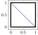
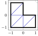
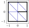
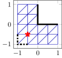
Figure 1: Initial triangulations $\mathcal{T}_{0}$ and boundary conditions (BC) ${\Gamma_{C}}$ () and ${\Gamma_{S}}$ () from left to right: the Square, the L-shape, and the Slit with homogeneous BC and the L-shape with mixed BC and point force ()

4.1 Numerical realisation

Enumerate the nodal basis $\{\varphi_{1},\dots,\varphi_{N}\}$ of $V(\mathcal{T})$ from (10) by $1$ to the number of degrees of freedom $N\coloneqq\mathrm{dim}(V(\mathcal{T}))$. The algebraic formulation of (3) writes $u_{h,0}=\sum_{j=1}^{N}x_{j}\varphi_{j}\in V(\mathcal{T})$ with coefficient vector $x\in{\mathbb{R}}^{N}$ and seeks $u_{h,0}=u_{h}-\mathcal{I}g$ such that

$$Ax=b$$ (19)

holds with the stiffness matrix and right-hand side vector

$$A \coloneqq(a(\varphi_{k},\varphi_{j}))_{k,j=1,\dots,N}\in{\mathbb{R}}^{N\times N}, b \coloneqq(F(\varphi_{j})-a(\mathcal{I}g,\varphi_{j}))_{j=1,\dots,N}\in{\mathbb{R}}^{N}.$$

The computation of $A$ and $b$ in the FEM fashion requires the evaluation of the $21$ local basis functions of the quintic Argyris finite element on each triangle $T\in\mathcal{T}$ at quadrature points. Possible approximation errors in the integration of non-polynomial expressions (e.g., from $f$ from (14) and $g$) by quadrature are expected to be small and are therefore neglected in this paper. The transformation from the reference element [21, 14] allows an efficient evaluation of the local basis on the physical element. Note that from the implementational viewpoint the hierarchical Argyris FEM only differs from the standard Argyris FEM in that it treats the global $\partial_{\zeta_{z},\zeta_{z}}^{2}\delta_{z}$ dof as the two degrees of freedom $\partial_{\zeta_{z},\zeta_{z}}^{2}\delta_{z}^{\pm}$ from (9) for every $z\in\mathcal{V}(\Omega)\setminus\mathcal{V}_{0}$. This section solves (19) with the direct solver mldivide from the MATLAB standard library that is behind the \ command.

4.2 Benchmarks with homogeneous boundary conditions

This benchmark for the plate equation with uniform load $F\equiv 1$ consider homogeneous clamped boundary conditions ($g\equiv 0$ and $\partial\Omega={\Gamma_{C}}$) on the Square ($\Omega=(0,1)^{2}$) and the L-shape ($\Omega=(-1,1)^{2}\setminus[0,1)^{2}$) with initial triangulations given in figure 1. Although the exact solution $u$ is unknown, the energy error of $u-u_{h}\in V$ can be computed by exploiting the Galerkin property for conforming discretisations, i.e.,

$$|\!|\!|u-u_{h}|\!|\!|^{2}=|\!|\!|u|\!|\!|^{2}-|\!|\!|u_{h}|\!|\!|^{2}.$$

The computation on a sufficiently fine mesh and multi-precision arithmetic led to the approximations $|\!|\!|u|\!|\!|^{2}=3.8912007750677\times 10^{-4}$ for the Square and $|\!|\!|u|\!|\!|^{2}=3.57857007158618\times 10^{-3}$ for the L-shape.

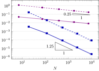
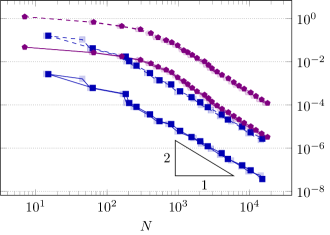
Figure 2: Convergence history of the standard (opaque) and hierarchical (filled) Argyris AFEM on the L-shape and Square with uniform (left) and adaptive (right, $\theta=0.5$) mesh-refinement

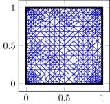
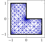
Figure 3: Adaptive triangulations $\mathcal{T}$ for $\theta=0.5$ of the $\mathfrak{A}_{\rm ext}$-AFEM on the Square ($|\mathcal{T}|=861$) and the L-shape ($|\mathcal{T}|=748$)

A uniform load on the L-shape with its corner singularity (at the origin) is the prototypical example of reduced convergence rates for a uniformly refined mesh-sequence. Figure 2 does not only show an empirical suboptimal rate of $-1/4$ in the number of degrees of freedom $N$ for the L-shape but also a reduced rate of ${-5/4}$ on the Square. This is shown for both the error in the energy norm $|\!|\!|u-u_{h}|\!|\!|$ and the error estimator $\eta(\mathcal{T}_{\ell})$ for the standard as well as the hierarchical Argyris FEM with uniform refinement. The reduced rates are due to corner singularities [1] of the solution $u$ and underline the necessity of adaptive schemes even on the convex Square.

Figure 3 shows refinement towards all (including convex) corners and a strong refinement towards the re-entering corner at the origin for the L-shape. Figure 2 also shows the theoretically predicted optimal convergence rates for the $\mathfrak{A}_{\rm ext}$-AFEM together with equivalence of the error estimator and the energy error. The same observations apply for the $\mathfrak{A}_{\rm std}$-AFEM.

4.3 Inhomogeneous boundary data on the Slit

This benchmark problem considers the non-Lipschitz Slit ($\Omega=(0,1)^{2}\setminus(\{0\}\times[0,1))$) with pure clamped boundary ${\Gamma_{C}}=\partial\Omega$. The boundary data $g=u$ and source $F\equiv 1$ match the exact solution (in polar coordinates)

$$u(r,\varphi) =-\frac{r^{2}}{16}\left(r^{1/2}\sin(\varphi/2)-\frac{r^{2}}{2}\sin^{2}(\varphi)\right).$$

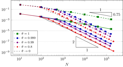
Figure 4: Convergence history of the standard (opaque) and hierarchical (filled) Argyris AFEM for different bulk parameter $\theta$

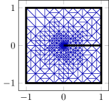
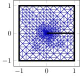
Figure 5: Adaptive triangulations $\mathcal{T}$ for $\theta=0.5$ of the $\mathfrak{A}_{\rm ext}$-AFEM (left, $|\mathcal{T}|=700$) and of the $\mathfrak{A}_{\rm std}$-AFEM (right, $|\mathcal{T}|=867$)

Despite the singularity at the origin, the derivatives $\nabla u,D^{2}u$ up to second order exist and vanish at the origin, hence the interpolation $\mathcal{I}u\in\mathfrak{A}(\mathcal{T})$ is well defined.

The theory on optimal convergence rates requires the bulk parameter $\theta$ to be sufficiently small. A first explicit computation [10, Ex. 6.3] of the theoretical quantities for the Courant FEM concludes optimality for $\theta\leq\Theta\coloneqq 2.6\times 10^{-6}$. It is generally accepted that $\theta=0.5$ leads to optimal convergence in most practical scenarios. Figure 4 shows optimal rates even for $\theta$ close to one where $\theta=1$ abbreviates uniform refinement and $\theta\to 0$ signals the opposite extreme with only $\mathrm{argmax}_{T\in\mathcal{T}}\eta(\mathcal{T},T)$ marked for refinement. A higher bulk parameter $\theta$ initially leads to broader refinement and fewer steps of the adaptive algorithm in the pre-asymptotic regime. Yet, a choice of $0.5\leq\theta\leq 0.999$ produces similar iterations for $N\geq 10^{3}$. Even smaller values $\theta\leq 0.1$ lead to more refinement steps throughout but do not significantly improve on $\theta=0.8$.

With the sole singularity of $u$ at the origin, figure 5 shows concentric refinement towards the origin. The adaptive mesh sequences obtained from $\mathfrak{A}_{\rm ext}$-AFEM and $\mathfrak{A}_{\rm std}$-AFEM are qualitatively the same.

4.4 Mixed boundary conditions and point load

In this benchmark the situation at hand is motivated by the biharmonic equation in the context of plate bending. Consider a quadratic floor in some building, e.g., skyscraper, made out of reinforced concrete. Suppose that the core of the building carries all the weight and that therefore the floor is embedded into the central square. Furthermore, there are supports around the outer corners that support the floor but do not fix tilting. Since the layout is symmetric, the further considerations are reduced to the lower left quarter so that the domain in consideration is represented by the L-shape with initial triangulation shown in figure 1. Displacement and bending are prescribed on ${\Gamma_{C}}=\{0\}\times[0,1)\cup[0,1)\times\{0\}$ whereas only displacement is fixed on ${\Gamma_{S}}=\{-1\}\times[-1/2,-1]\cup[-1,-1/2]\times\{-1\}$.

A point load $F=\delta_{z}\in H^{-2}(\Omega)$ at $z=(-1/2,-1/2)$ leads to a situation of no known solution $u$ to the biharmonic equation

$$\Delta^{2}u=\delta_{z}$$

with boundary data $g=10^{-3}\sin(\kappa x^{3}y^{3}\pi)$ introducing oscillations through $\kappa\geq 0$.

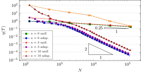
Figure 6: Convergence history for different values of $\kappa=0,3,10$

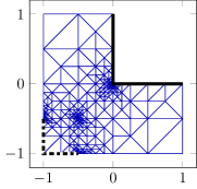
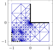
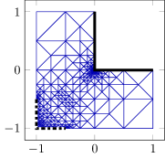
Figure 7: Adaptive triangulations $\mathcal{T}$ from left to right; for $\kappa=0$ ($|\mathcal{V}|=367$), for $\kappa=3$ ($|\mathcal{V}|=372$), and for $\kappa=10$ ($|\mathcal{V}|=340$)

Mixed boundary conditions and the fact $F\not\in H^{-1}(\Omega)$ (but $F\in H^{-1-\varepsilon}(\Omega)$ for $0<\varepsilon<1$) result in a problem with multiple singularities of different magnitude where the a priori mesh generation is not at all clear. The adaptive algorithm leads to optimal rates for the standard and hierarchical Argyris AFEM, see figure 6 for $\kappa=0,3,10$. A large value of $\kappa$ introduces strong oscillations of the boundary data on ${\Gamma_{S}}$. This initially leads to strong refinement on ${\Gamma_{S}}$ while the refinement for small $\kappa\geq 0$ concentrates on the location of the point force $z$, the origin, and the boundary of ${\Gamma_{S}}$. Figure 7 shows these different intensities of the refinement for $\kappa=0,3,10$ on triangulations of the $\mathfrak{A}_{\rm ext}$-AFEM algorithm with $\theta=0.5$. In fact, large parts, away from the singularities, were not further refined at all. Anyhow, the oscillations of the boundary data are of higher order, see lemma 2.3, so that their impact on uniform triangulations becomes negligible for a small maximal mesh-size.

5 AFEM with iterative multilevel solver

This section compares the direct solver (from section 4) with the iterative multigrid (MG) and preconditioned conjugated gradient (PCG) methods for the solution to (3) of the hierarchical Argyris AFEM ($\mathfrak{A}_{\rm ext}$-AFEM). Throughout this section, the index $\ell$ refers to the level $\ell\in{\mathbb{N}}_{0}$ some object is associated with.

5.1 Adaptive multigrid V-cycle

Consider a sequence of successive refinements $(\mathcal{T}_{\ell})_{\ell}$ with stiffness matrix $A_{\ell}$ and right-hand side vector and $b_{\ell}$ at level $\ell\in{\mathbb{N}}_{0}$. Recall the nodal basis $\{\varphi^{\ell}_{j}\}_{\ell=1}^{N_{\ell}}$ for the discrete test space $V(\mathcal{T}_{\ell})$ of dimension $N_{\ell}\coloneqq\mathrm{dim}(V(\mathcal{T}_{\ell}))$ and the algebraic formulation $A_{\ell}x_{\ell}=b_{\ell}$ of (3) from subsection 4.1. Multigrid methods make use of the whole sequence of discretisations to solve $A_{\ell}x_{\ell}=b_{\ell}$. The matrix version [2] of the multigrid V-cycle for the hierarchical Argyris FEM [11, Sec. 5] requires the prolongation matrix $P_{\ell}\in{\mathbb{R}}^{N_{\ell}\times N_{\ell}-1}$ that expresses a coarse function in terms of the fine basis functions, i.e., $\varphi_{k}^{\ell-1}=\sum_{j=1}^{N_{\ell}}P_{\ell,jk}\varphi^{\ell}_{j}$ for $1\leq k\leq N_{\ell-1}$, and the matrix $S_{\ell}\in{\mathbb{R}}^{N_{\ell}\times N_{\ell}}$. Let $I_{\ell}\coloneqq\{j\ :\ \varphi^{\ell}_{j}\not\in V(\mathcal{T}_{\ell-1})\}$ denote the indices of the new basis functions at level $\ell$. The local Gauß-Seidel smoother $S_{\ell}$ acts on the $I_{\ell}$-components of a vector $y_{\ell}\in{\mathbb{R}}^{N_{\ell}}$ by

$$(S_{\ell}y_{\ell})_{j}\coloneqq\begin{cases}{}(\tilde{A}_{\ell}^{-1}y_{\ell|I_{\ell}})_{j}&\text{ if }j\in I_{\ell},\\ 0&\text{ else,}\end{cases}$$ (20)

where $\tilde{A}_{\ell}=\mathrm{tril}(A_{\ell|I_{\ell}I_{\ell}})$ denotes the lower triangular part (including the diagonal) of the submatrix $A_{\ell|I_{\ell}I_{\ell}}=(A_{\ell,kj})_{k,j\in I_{\ell}}$ and $y_{\ell|I_{\ell}}=(y_{\ell,j})_{j\in I_{\ell}}$, see [3] for the relation with the operator notation of $S_{\ell}$ in [11]. This way, $S_{\ell}$ only acts on the components that correspond to new basis functions (either associated to a new node $z\in\mathcal{N}_{\ell}\setminus\mathcal{N}_{\ell-1}$ or with support on a refined triangle $T\in\mathcal{T}_{\ell}\setminus\mathcal{T}_{\ell-1}$).

Input: $y_{\ell}\in V(\mathcal{T}_{\ell}),r\in{\mathbb{N}}$

if $\ell=0$ then

     Exact solve: $B_{0}y_{0}=A_{0}^{-1}y_{0}$

else

     Pre-smoothing: $w_{j+1}\coloneqq w_{j}+S_{\ell}(y_{\ell}-A_{\ell}w_{j})$ for $w_{0}\coloneqq 0$ and $j=0,\dots,r-1$

     Coarse-grid correction: $w_{r+1}\coloneqq w_{r}+P_{\ell}B_{\ell-1}P_{\ell}^{\top}(y_{\ell}-A_{\ell}w_{r})$

     Post-smoothing: $w_{j+1}\coloneqq w_{j}+S_{\ell}^{\top}(y_{\ell}-A_{\ell}w_{j})$ for $j=r+1,\dots,2r$

     Set $B_{\ell}y_{\ell}\coloneqq w_{2r+1}$.

end if

Output: $B_{\ell}y_{\ell}$

Algorithm 2 (V$(r)$-cycle)

The standard symmetric multigrid V-cycle [2], algorithm 2, with $r$ pre- and post-smoothing steps defines a uniform approximative inverse $B_{\ell}$ of $A_{\ell}$ in the spectral energy norm $|\!|\!|M|\!|\!|_{2}\coloneqq\sup_{y_{\ell}\in{\mathbb{R}}^{N_{\ell}}\setminus 0}(y_{\ell}^{\top}A_{\ell}My_{\ell})/(y_{\ell}^{\top}A_{\ell}y_{\ell})$ for $M\in{\mathbb{R}}^{N_{\ell}\times N_{\ell}}$. The original proof for the $V(1)$-cycle holds for general $V(r)$-cycles.

Theorem 5.1 ([11, Thm. 7]).

For the $\mathfrak{A}_{\rm ext}$-AFEM, there exists $c_{\infty}\in{\mathbb{R}}$ with

$$\sup_{\ell\in{\mathbb{N}}_{0}}|\!|\!|I-B_{\ell}A_{\ell}|\!|\!|_{2}\leq\frac{c_{\infty}}{1+c_{\infty}}<1.$$

Proof.

Notice, e.g., from [2, Sec. 10] and [18, Sec. 3], that $S_{\ell}$ and $P^{\top}_{\ell}$ are the matrix representations of the local Gauß-Seidel relaxation operator in [11] and the $L^{2}$ projection $V(\mathcal{T}_{\ell})\to V(\mathcal{T}_{\ell-1})$. This establishes $I-B_{\ell}A_{\ell}$ as the matrix representation of the operator $I-\mathcal{B}_{\ell}\mathcal{A}_{\ell}$ from [11, Sec. 7.6]. The proof of [11, Thm. 7] provides $I-\mathcal{B}_{\ell}\mathcal{A}_{\ell}=\mathcal{R}^{*}\mathcal{R}$ with $\mathcal{R}=(I-\mathcal{P}_{0})\prod_{j=1}^{\ell}(I-\mathcal{Q}_{j})^{r}$ for $r$ smoothing steps and operators $\mathcal{P}_{0},\mathcal{Q}_{j},j=1,\dots,\ell$. The application of [29] provides $c_{\ell}^{(r)}\in{\mathbb{R}}$ with

$$\|I-\mathcal{B}_{\ell}\mathcal{A}_{\ell}\|_{\mathcal{A}_{\ell}}\coloneqq\sup_{v_{\ell}\in V(\mathcal{T}_{\ell})\setminus 0}\frac{a((I-\mathcal{B}_{\ell}\mathcal{A}_{\ell})v_{\ell},v_{\ell})}{a(v_{\ell},v_{\ell})}=\|\mathcal{R}\|_{\mathcal{A}_{\ell}}^{2}=\frac{c_{\ell}^{(r)}}{1+c_{\ell}^{(r)}}.$$ (21)

The explicit characterisation of $c_{\ell}^{(r)}\in{\mathbb{R}}$ shows $c_{\ell}^{(r)}\leq c_{\ell}^{(1)}\leq c_{\infty}$ with the uniform bound $c_{\infty}\in{\mathbb{R}}$ [11, Thm. 7] and concludes the proof for general $r\in{\mathbb{N}}$. ∎

5.2 Stopping criterion

Let $x_{\ell}\in{\mathbb{R}}^{N_{\ell}}$ denote the exact solution to (19), i.e., $u_{\ell}=u_{\ell,0}+\mathcal{I}_{\ell}g$ solves (3) for $u_{\ell,0}=\sum_{j=1}^{N_{\ell}}x_{j}\varphi^{\ell}_{j}$. For any $\tilde{u}_{\ell}=\tilde{u}_{\ell,0}+\mathcal{I}_{\ell}g$ with coefficient vector $\tilde{x}_{\ell}\in{\mathbb{R}}^{N_{\ell}}$ of $\tilde{u}_{\ell,0}\in V(\mathcal{T}_{\ell})$, a reliable and efficient estimator

$$\eta_{\rm alg}(\mathcal{T}_{\ell},\tilde{x}_{\ell})\coloneqq\left((b_{\ell}-A_{\ell}\tilde{x}_{\ell})^{\top}B_{\ell}(b_{\ell}-A_{\ell}\tilde{x}_{\ell})\right)^{1/2}$$

for the algebraic error $|\!|\!|u_{\ell}-\tilde{u}_{\ell}|\!|\!|$ comes from the approximate inverse $B_{\ell}$ of the multigrid V-cycle. This motivates the stopping criterion with tolerance $0<tol$ for initial solution $\tilde{x}_{\ell}^{0}\in{\mathbb{R}}^{N_{\ell}}$,

$$\eta_{\rm alg}(\mathcal{T}_{\ell},\tilde{x}_{\ell})<tol\;\eta_{\rm alg}(\mathcal{T}_{\ell},\tilde{x}_{\ell}^{0}).$$ (22)

Lemma 5.2 ([18, Lem. 3.5]).

If $|\!|\!|I-B_{\ell}A_{\ell}|\!|\!|_{2}\leq C<1$, then for any $\tilde{u}_{\ell,0}\in V(\mathcal{T}_{\ell})$ with coefficient vector $\tilde{x}_{\ell}\in{\mathbb{R}}^{N_{\ell}}$ and $\tilde{u}_{\ell}\coloneqq\tilde{u}_{\ell,0}+\mathcal{I}_{\ell}g\in\mathfrak{A}_{\rm ext}(\mathcal{T})$,

$$(1-C)^{1/2}|\!|\!|u_{\ell}-\tilde{u}_{\ell}|\!|\!|\leq\eta_{\rm alg}(\mathcal{T}_{\ell},\tilde{x}_{\ell})\leq(1+C)^{1/2}|\!|\!|u_{\ell}-\tilde{u}_{\ell}|\!|\!|.$$

Proof.

With the error $e_{\ell}\coloneqq x_{\ell}-\tilde{x}_{\ell}$, the residual reads $A_{\ell}e_{\ell}=b_{\ell}-A_{\ell}\tilde{x}_{\ell}$ and

$$|\!|\!|u_{\ell}-\tilde{u}_{\ell}|\!|\!|^{2}\coloneqq a(u_{\ell,0}-\tilde{u}_{\ell,0},u_{\ell,0}-\tilde{u}_{\ell,0})=e_{\ell}^{\top}A_{\ell}e_{\ell}=e_{\ell}^{\top}A_{\ell}(I-B_{\ell}A_{\ell})e_{\ell}+e_{\ell}^{\top}A_{\ell}B_{\ell}A_{\ell}e_{\ell}.$$ (23)

The definition of the norm, $|\!|\!|I-B_{\ell}A_{\ell}|\!|\!|_{2}\leq C$, and $\eta_{\rm alg}(\mathcal{T}_{\ell},\tilde{x}_{\ell})=e_{\ell}^{\top}A_{\ell}B_{\ell}A_{\ell}e_{\ell}$ show

$$|\!|\!|u_{\ell}-\tilde{u}_{\ell}|\!|\!|^{2} \leq C\;|\!|\!|u_{\ell}-\tilde{u}_{\ell}|\!|\!|^{2}+\eta_{\rm alg}(\mathcal{T}_{\ell},\tilde{x}_{\ell}).$$

This proves the first inequality and the second follows by similar arguments after rearranging (23). ∎

This section applies the (full) multigrid method (MG) with iterations

$$\tilde{x}_{\ell}^{j+1}=\tilde{x}_{\ell}^{j}+B_{\ell}(b_{\ell}-A_{\ell}\tilde{x}_{\ell}^{j})$$

and the preconditioned conjugated gradient method (PCG) with preconditioner $B_{\ell}$ as an example for Krylov subspace methods [24]. The stopping criterion reads (22) and the initial solution $\tilde{x}_{\ell}^{0}$ is the coefficient vector of the solution at the previous level $u_{\ell-1,0}$ for $\ell\geq 1$ or $\tilde{x}_{0}^{0}\coloneqq 0$; this is also known as nested iterations.

Remark (alternative stopping criterion).

Gantner et al. [15] discuss an alternative stopping criterion that requires the evaluation of the error estimator $\eta(\mathcal{T}_{\ell})$ at $\tilde{u}_{\ell}$ for each iteration and prove optimal rates of the overall adaptive algorithm (given a small enough tolerance). In practice however, the evaluation of the error estimator $\eta(\mathcal{T}_{\ell})$ from (15) by quadrature dominates the computational time in the solve step of algorithm 1.

The computation of the stopping criterion (22) in this paper is remarkably simple as the MG-update $B_{\ell}(b_{\ell}-A_{\ell}\tilde{x}_{\ell})$ and the residual $b_{\ell}-A_{\ell}\tilde{x}_{\ell}$ are already computed quantities of each MG or PCG iteration.

5.3 Adaptive algorithm with inexact solve

A crucial ingredient in the proof of reliability of the error estimator $\eta(\mathcal{T})$ is the Galerkin property

$$|\!|\!|u-v_{h}|\!|\!|^{2}=|\!|\!|u-u_{h}|\!|\!|^{2}+|\!|\!|u_{h}-v_{h}|\!|\!|^{2}$$ (24)

of the exact discrete solution $u_{h}$ to (3) and any $v_{h}\in\mathcal{I}g+V(\mathcal{T})$. For an approximation $\tilde{u}_{h}\in\mathcal{I}g+V(\mathcal{T})$ to $u_{h}$ this generally does not hold but shows that the discretisation error $u-u_{h}$ is $a$-orthogonal to the algebraic error $u_{h}-\tilde{u}_{h}$. Since $\eta(\mathcal{T})$ depends continuously on $u_{h}$, a small algebraic error $|\!|\!|u_{h}-\tilde{u}_{h}|\!|\!|$ is acceptable and leads to optimal rates of the $\mathfrak{A}_{\rm ext}$-AFEM algorithm 1 with inexact solve, see figure 8 for the Slit benchmark B3 from subsection 4.3. For too coarse approximations ($tol=0.7$ in fig. 8), the algebraic error does not converge with optimal rate and, thus by (24), the same holds true for the total error $|\!|\!|u-\tilde{u}_{h}|\!|\!|$. In this case, the error estimator $\eta(\mathcal{T})$, evaluated for $\tilde{u}_{h}$, is not reliable and suggests a better convergence rate. Conversely, further (undisplayed) experiments with the benchmarks from section 4 suggest that an optimal convergence of the algebraic error $|\!|\!|u_{h}-\tilde{u}_{h}|\!|\!|$ is also sufficient for reliability of $\eta(\mathcal{T})$. Hence, $\eta_{\rm alg}(\mathcal{T},\tilde{x}_{h})$ (equivalent to $|\!|\!|u_{h}-\tilde{u}_{h}|\!|\!|$ by lemma 5.2 and theorem 5.1) serves as an indicator for optimal rates.

Undisplayed numerical experiments with the related adaptive scheme from [15] show a very similar convergence behaviour and dependence on the tolerance of the stopping criterion compared to (22). This hints at a possible equivalence of both algorithms and motivates further investigations regarding a convergence analysis extending [15] to inhomogeneous boundary data.

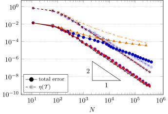
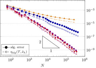
Figure 8: Convergence history of the total error $|\!|\!|u-\tilde{u}_{h}|\!|\!|$ (solid) and $\eta(\mathcal{T})$ (dashed) for AFEM ($\theta=0.8$) using iterative multigrid (MG) and preconditioned CG (PCG) solvers compared with the direct solver for the Slit benchmark (B3)

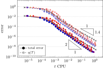
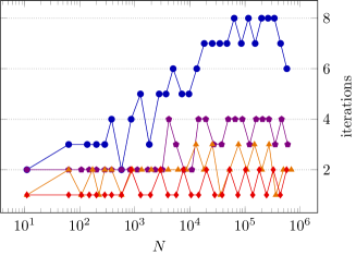
Figure 9: Convergence history of the total error $|\!|\!|u-\tilde{u}_{h}|\!|\!|$ (solid) and $\eta(\mathcal{T})$ (dashed) against the single-core CPU time $t$ of one MG/PCG iteration in seconds on Intel^® Xeon^® Gold 5222 CPU at 3.80GHz with 1000GB RAM (left) and the number of iterations (right) with $tol=0.1$ for the Slit benchmark (B3)

5.4 Linear time complexity AFEM

Algorithm 1 consists of the steps Solve, Estimate, Mark and Refine. Each of these steps has a linear time complexity (in the number of degrees of freedom $N$) if an appropriate solver is applied in the Solve step, see [23] for the linear complexity of Dörfler marking with minimal cardinality. Direct solvers do not allow for a linear time complexity. Nevertheless, they still perform well in some situations [16]. On the contrary, iterative methods may archive a linear time complexity if the number of iterations is uniformly bounded and each iteration is of linear complexity. Work estimates [2] prove this for the multigrid $V(r)$-cycle under the assumption of an (asymptotically) exponential growth in the degrees of freedom, i.e., $N_{\ell+1}\geq aN_{\ell}$ for some $a>1$.

The numerical benchmarks indeed verify a linear $\mathcal{O}(N)$ time complexity of the iterative MG and PCG solvers and a superlinear growth of approximately $\mathcal{O}(N^{1.4})$ for the direct solver. Figure 9 verifies the uniform bound on the number of iterations for MG and PCG with the $V(r)$-cycle for $r=1,2,5$. This results in observed optimal convergence rates of the total error $|\!|\!|u-\tilde{u}_{h}|\!|\!|$ as well as the error estimator $\eta(\mathcal{T})$ with respect to the computational time in seconds for the iterative schemes and the experimental convergence rate $1.4$ for AFEM with direct solve. For the shown benchmark B3, the PCG method with a single $r=1$ smoothing iteration performs the best and obtains the solution to (19) faster than the direct solver on fine meshes with more than $3\times 10^{4}$ degrees of freedom.

5.5 Norm of the multigrid iteration matrix

The norm of the multigrid iteration matrix $I-B_{\ell}A_{\ell}$ quantifies the convergence rate of the multigrid method and control over it as in theorem 5.1 leads to uniform convergence. Given $\ell\in{\mathbb{N}}$, it is known that

$$C\coloneqq|\!|\!|I-B_{\ell}A_{\ell}|\!|\!|_{2}=c/(1+c)$$ (25)

for some $c\in{\mathbb{R}}$, see the proof of theorem 5.1. The Rayleigh-Ritz principle (also known as the min-max principle) for the symmetric matrices $A_{\ell}$ and $A_{\ell}(I-B_{\ell}A_{\ell})$ shows that the spectral energy norm $|\!|\!|I-B_{\ell}A_{\ell}|\!|\!|_{2}$ of the iteration matrix is equal to the maximal eigenvalue of $I-B_{\ell}A_{\ell}$. Figure 10 displays the history of $|\!|\!|I-B_{\ell}A_{\ell}|\!|\!|_{2}$, computed with eigs from the MATLAB standard library (and $B_{\ell}$ provided as a function handle) and shows that $|\!|\!|I-B_{\ell}A_{\ell}|\!|\!|_{2}$ is clearly bounded away from one. Since the work in one $V(r)$-cycle is roughly equal to that of $r$ $V(1)$-cycles, it is expected that the number of iterations correlates anti-proportionally to the number of smoothing steps $r$. Table 3 collects the values of $C,c$ from (25), and the number of iterations n_it on a fine mesh from the multigrid $\mathfrak{A}_{\rm ext}$-AFEM with $r$ smoothing steps and verifies this expectation.

$r$	Square (B1)			L-shape (B2)			Slit (B3)
	$C$	$c$	n_it	$C$	$c$	n_it	$C$	$c$	n_it
$1$	0.9014	9.14	2	0.9590	23.39	12	0.9339	14.13	8
$2$	0.5774	1.36	1	0.9096	10.06	6	0.8608	6.18	4
$3$	0.3701	0.58	1	0.8666	6.49	4	0.8070	4.18	3
$5$	0.1949	0.24	1	0.8022	4.06	3	0.7157	2.52	2

Table 3: Values of $C\coloneqq|\!|\!|I-B_{\ell}A_{\ell}|\!|\!|_{2}$ for the multigrid AFEM ($\theta=0.5$) on meshes with more than $2\cdot 10^{5}$ degrees of freedom

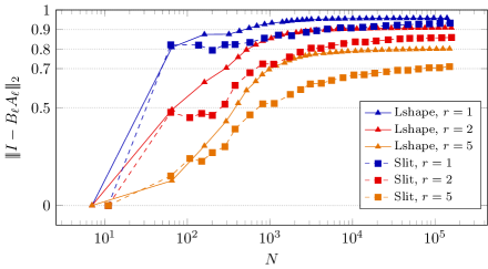
Figure 10: History of $|\!|\!|I-B_{\ell}A_{\ell}|\!|\!|_{2}$ from the multigrid AFEM for B2 (L-shape) and B3 (Slit) from subsections 4.2 and 4.3

6 Concluding remarks

A comparison between the classical and the extended Argyris space in section 4 shows qualitatively similar mesh sequences and convergence. The extended Argyris space comes with about $11$% more degrees of freedom compared to the standard Argyris space on the same mesh. This extra amount of computation stands opposed to the availability of theoretically justified, local multilevel preconditioned solvers and an easily computable, reliable, and efficient estimator of the algebraic error. Moreover, section 5 finds the $\mathfrak{A}_{\rm ext}$-AFEM algorithm with inexact solve highly efficient and of linear time complexity in the overall computational cost. The linear space (memory) complexity of the local multilevel scheme is another advantage over classical direct solvers [16] that becomes important on systems with limited memory. A possible extension to the standard Argyris FEM requires a different prolongation as no natural injection from coarse to fine spaces exists. Theoretical results for the related adaptive algorithm are not available (see [4] for multigrid on quasi-uniform meshes).

The local Gauß-Seidel smoother only acts on the refined portion of the mesh. A simple MATLAB implementation was found competitive with the highly optimised direct solver and the PCG solver is already faster on meshes with $3\times 10^{4}$ degrees of freedom. The alternative application of the standard Gauß-Seidel (also known as multiplicative) smoother that acts on the full set of degrees of freedom shows no qualitative reduction in the number of iterations and comes with an additional computational cost. This extra cost can be efficiently circumvented with local smoothing, see also [28], considered in this paper.

A possible (uniform) convergence rate of the multigrid iteration close to one does not spoil the application of multilevel preconditioned methods in the adaptive setting, as the moderate number of iterations in table 3 suggests. In fact, the PCG method with a single smoothing step only required between $1$ and $4$ iterations throughout.

The hierarchical Argyris FEM marks a paradigm shift in the approximation of conforming fourth-order problems away from minimising the dimension of the discrete spaces towards justifying higher order methods. Numerical benchmarks reestablish the Argyris element with high convergence rates, an easy implementation by transformation [14, 21], and an overall linear time complexity of the optimal adaptive algorithm.

References

- Blum and Rannacher [1980] Blum, H., Rannacher, R., 1980. On the boundary value problem of the biharmonic operator on domains with angular corners. Mathematical Methods in the Applied Sciences 2 (4), 556–581.
- Bramble [1993] Bramble, J. H., 1993. Multigrid methods. No. 294 in Pitman research notes in mathematics series. Longman Scientific & Technical; Wiley, Harlow, Essex, England : New York.
- Bramble and Pasciak [1992] Bramble, J. H., Pasciak, J. E., May 1992. The analysis of smoothers for multigrid algorithms. Math. Comp. 58 (198), 467–467.
- Bramble and Zhang [1995] Bramble, J. H., Zhang, X., Jan. 1995. Multigrid methods for the biharmonic problem discretized by conforming C finite elements on nonnested meshes. Numerical Functional Analysis and Optimization 16 (7-8), 835–846.
- Brenner and Carstensen [2017] Brenner, S. C., Carstensen, C., Dec. 2017. Finite element methods. In: Stein, E., de Borst, R., Hughes, T. J. R. (Eds.), Encyclopedia of Computational Mechanics Second Edition. John Wiley & Sons, Ltd, Chichester, UK, pp. 1–47.
- Brenner and Scott [2008] Brenner, S. C., Scott, L. R., 2008. The mathematical theory of finite element methods. Vol. 15 of Texts in Applied Mathematics. Springer New York, New York, NY.
- Brezis and Mironescu [2018] Brezis, H., Mironescu, P., 2018. Gagliardo-Nirenberg inequalities and non-inequalities: the full story. Annales de l’Institut Henri Poincaré (C) Non Linear Analysis 35 (5), 1355–1376.
- Carstensen et al. [2014a] Carstensen, C., Feischl, M., Page, M., Praetorius, D., Apr. 2014a. Axioms of adaptivity. Computers & Mathematics with Applications 67 (6), 1195–1253.
- Carstensen et al. [2014b] Carstensen, C., Gallistl, D., Hu, J., Dec. 2014b. A discrete Helmholtz decomposition with Morley finite element functions and the optimality of adaptive finite element schemes. Computers & Mathematics with Applications 68 (12), 2167–2181.
- Carstensen and Hellwig [2018] Carstensen, C., Hellwig, F., Jul. 2018. Constants in discrete Poincaré and Friedrichs inequalities and discrete quasi-interpolation. Computational Methods in Applied Mathematics 18 (3), 433–450.
- Carstensen and Hu [2021] Carstensen, C., Hu, J., Jul. 2021. Hierarchical Argyris finite element method for adaptive and multigrid algorithms. Computational Methods in Applied Mathematics 21 (3), 529–556.
- Carstensen and Rabus [2017] Carstensen, C., Rabus, H., Jan. 2017. Axioms of adaptivity with separate marking for data resolution. SIAM J. Numer. Anal. 55 (6), 2644–2665.
- Ciarlet [2002] Ciarlet, P. G., Jan. 2002. The finite element method for elliptic problems. Classics in Applied Mathematics. Society for Industrial and Applied Mathematics.
- Domínguez and Sayas [2008] Domínguez, V., Sayas, F.-J., Jul. 2008. Algorithm 884: A simple matlab implementation of the Argyris element. ACM Trans. Math. Softw. 35 (2), 1–11.
- Gantner et al. [2021] Gantner, G., Haberl, A., Praetorius, D., Schimanko, S., Jun. 2021. Rate optimality of adaptive finite element methods with respect to overall computational costs. Math. Comp. 90 (331), 2011–2040.
- George and Ng [1988] George, A., Ng, E., Sep. 1988. On the complexity of sparse QR and LU factorization of finite-element matrices. SIAM J. Sci. and Stat. Comput. 9 (5), 849–861.
- Girault and Scott [2002] Girault, V., Scott, L. R., Jan. 2002. Hermite interpolation of nonsmooth functions preserving boundary conditions. Math. Comp. 71 (239), 1043–1074.
- Gräßle [2022] Gräßle, B., 2022. Conforming multilevel FEM for the biharmonic equation. Master’s thesis, Humboldt-Universität zu Berlin, Mathematisch-Naturwissenschaftliche Fakultät.
- Grisvard [1992] Grisvard, P., 1992. Singularities in boundary value problems. No. 22 in Research notes in applied mathematics. Masson, Paris.
- Karkulik et al. [2013] Karkulik, M., Pavlicek, D., Praetorius, D., Oct. 2013. On 2D newest vertex bisection: optimality of mesh-closure and -stability of -projection. Constr Approx 38 (2), 213–234.
- Kirby [2018] Kirby, R. C., Apr. 2018. A general approach to transforming finite elements. The SMAI journal of computational mathematics 4, 197–224.
- Payne and Weinberger [1960] Payne, L. E., Weinberger, H. F., Jan. 1960. An optimal Poincaré inequality for convex domains. Arch. Rational Mech. Anal. 5 (1), 286–292.
- Pfeiler and Praetorius [2020] Pfeiler, C.-M., Praetorius, D., Jun. 2020. Dörfler marking with minimal cardinality is a linear complexity problem. Math. Comp. 89 (326), 2735–2752.
- Saad [2003] Saad, Y., Jan. 2003. Iterative methods for sparse linear systems, 2nd Edition. Society for Industrial and Applied Mathematics.
- Stevenson [2008] Stevenson, R., Jan. 2008. The completion of locally refined simplicial partitions created by bisection. Math. Comp. 77 (261), 227–241.
- Sweers [2009] Sweers, G., Feb. 2009. A survey on boundary conditions for the biharmonic. Complex Variables and Elliptic Equations 54 (2), 79–93.
- Verfürth [2013] Verfürth, R., Apr. 2013. A posteriori error estimation techniques for finite element methods. Oxford University Press.
- Wu and Chen [2006] Wu, H., Chen, Z., Oct. 2006. Uniform convergence of multigrid V-cycle on adaptively refined finite element meshes for second order elliptic problems. SCI CHINA SER A 49 (10), 1405–1429.
- Xu and Zikatanov [2002] Xu, J., Zikatanov, L., Apr. 2002. The method of alternating projections and the method of subspace corrections in Hilbert space. J. Amer. Math. Soc. 15 (3), 573–597.