Computing roadmaps in unbounded smooth real algebraic sets I: connectivity results

Abstract

Answering connectivity queries in real algebraic sets is a fundamental problem in effective real algebraic geometry that finds many applications in e.g. robotics where motion planning issues are topical. This computational problem is tackled through the computation of so-called roadmaps which are real algebraic subsets of the set $V$ under study, of dimension at most one, and which have a connected intersection with all semi-algebraically connected components of $V$. Algorithms for computing roadmaps rely on statements establishing connectivity properties of some well-chosen subsets of $V$, assuming that $V$ is bounded.

In this paper, we extend such connectivity statements by dropping the boundedness assumption on $V$. This exploits properties of so-called generalized polar varieties, which are critical loci of $V$ for some well-chosen polynomial maps.

1 Introduction

Let $\mathbf{Q}$ be a real field of real closure $\mathbf{R}$ and let $\mathbf{C}$ be its algebraic closure (one can think about $\mathbb{Q}$, $\mathbb{R}$ and $\mathbb{C}$ instead, for the sake of understanding) and let $n\geq 0$ be an integer. An algebraic set $V\subset\mathbf{C}^{n}$ defined over $\mathbf{Q}$ is the solution set in $\mathbf{C}^{n}$ to a system of polynomial equations in $n$ variables with coefficients in $\mathbf{Q}$. A real algebraic set defined over $\mathbf{Q}$ is the set of solutions in $\mathbf{R}^{n}$ to a system of polynomial equations in $n$ variables with coefficients in $\mathbf{Q}$. It is also the real trace $V\cap\mathbf{R}^{n}$ of an algebraic set $V\subset\mathbf{C}^{n}$. Real algebraic sets have finitely many connected components [7, Theorem 2.4.4.]. Counting these connected components [17, 27] or answering connectivity queries over $V\cap\mathbf{R}^{n}$ [25] finds many applications in e.g. robotics [8, 12, 28, 21, 14].

Following [8, 10], such computational issues are tackled by computing a real algebraic subset of $V\cap\mathbf{R}^{n}$, defined over $\mathbf{Q}$, which has dimension at most one and a connected intersection with all connected components of $V$ and contains the input query points. In [8], Canny called such a subset a roadmap of $V$.

The effective construction of roadmaps, given a defining system for $V$, relies on connectivity statements which allow one to define real algebraic subsets of $V\cap\mathbf{R}^{n}$, of smaller dimension than that of $V\cap\mathbf{R}^{n}$, and that have a connected intersection with the connected components of $V\cap\mathbf{R}^{n}$. Such existing statements in the literature make the assumption that $V$ has finitely many singular points and $V\cap\mathbf{R}^{n}$ is bounded. In this paper, we focus on the problem of obtaining similar statements by dropping the boundedness assumption. We prove a new connectivity statement which generalizes the one of [24] to the unbounded case and will be used in a separate paper to obtain asymptotically faster algorithms for computing roadmaps. We start by recalling the state-of-the-art connectivity statement, which allows us to introduce some material we need to state our main result.

State-of-the-art overview

We start by introducing some terminology. Recall that an algebraic set $V\subset\mathbf{C}^{n}$ is the set of solutions of a finite system of polynomials equations. It can be uniquely decomposed into finitely many irreducible components. When all these components have the same dimension $d$, we say that $V$ is $d$-equidimensional. Those points ${\bm{y}}\in V$ at which the Jacobian matrix of a finite set of generators of its associated ideal has rank $n-d$ are called regular points and the set of those points is denoted by $\operatorname{reg}(V)$. The others are called singular points; the set of singular points of $V$ (its singular locus) is denoted by $\operatorname{sing}(V)$ and is an algebraic subset of $V$. We refer to [26] for definitions and propositions about algebraic sets.

A semi-algebraic set $S\subset\mathbf{R}^{n}$ is the set of solutions of a finite system of polynomial equations and inequalities. We say that $S$ is semi-algebraically connected if for any ${\bm{y}},{\bm{y}}^{\prime}\in S$, ${\bm{y}}$ and ${\bm{y}}^{\prime}$ can be connected by a semi-algebraic path in $S$, that is a continuous semi-algebraic function $\gamma\colon[0,1]\to S$ such that $\gamma(0)={\bm{y}}$ and $\gamma(1)={\bm{y}}^{\prime}$. A semi-algebraic set $S$ can be decomposed into finitely many semi-algebraically connected components which are semi-algebraically connected semi-algebraic sets that are both closed and open in $S$. Finally, for a semi-algebraic set $S\subset\mathbf{R}^{n}$, we denote by $\overline{S}$ its closure for the Euclidean topology on $\mathbf{R}^{n}$. We refer to [4] and [7] for definitions and propositions about semi-algebraic sets and functions.

Let $0\leq d\leq n$ and $V\subset\mathbf{C}^{n}$ be a $d$-equidimensional algebraic set such that $\operatorname{sing}(V)$ is finite. For $1\leq i\leq n$, let $\pi_{i}$ be the canonical projection:

$$\pi_{i}\colon({\bm{y}}_{1},\dotsc,{\bm{y}}_{n})\>\longmapsto\>({\bm{y}}_{1},\dotsc,{\bm{y}}_{i})$$

For a polynomial map $\bm{\varphi}\colon\mathbf{C}^{n}\rightarrow\mathbf{C}^{m}$ a point ${\bm{y}}\in V$ is a critical point of $\bm{\varphi}$ if ${\bm{y}}\in\operatorname{reg}(V)$ and the differential of the restriction of $\varphi$ to $V$ at ${\bm{y}}$, denoted by $d_{\bm{y}}\bm{\varphi}$, is not surjective, that is

$$d_{\bm{y}}\bm{\varphi}(T_{\bm{y}}V)\subsetneq\mathbf{C}^{m},$$

where $T_{\bm{y}}V$ denoted the tangent space to $V$ at ${\bm{y}}$. We will denote by $W^{\circ}(\bm{\varphi},V)$ the set of the critical points of $\bm{\varphi}$ on $V$. A critical value is the image of a critical point. We put $K(\bm{\varphi},V)=W^{\circ}(\bm{\varphi},V)\cup\operatorname{sing}(V)$. The points of $K(\bm{\varphi},V)$ are called the singular points of $\bm{\varphi}$ on $V$. Figure 1 show examples of such critical loci.

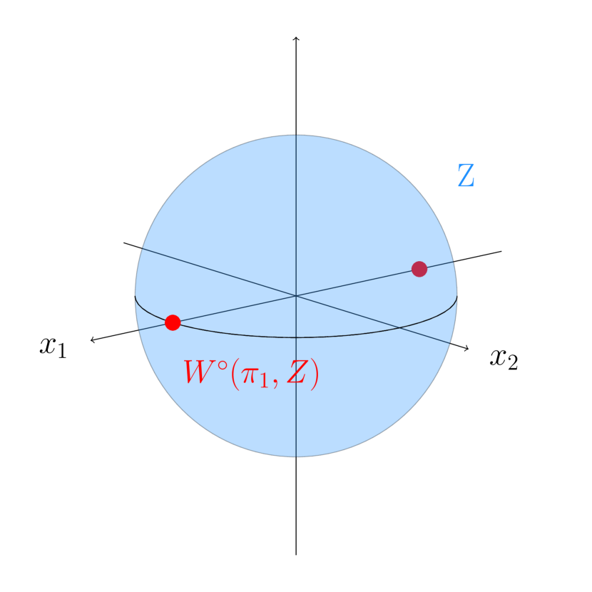
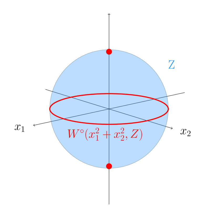
Figure 1: Real trace of the critical locus on a sphere $Z$ for: the projection on the first coordinate $\pi_{1}$ (left); the polynomial map $\varphi$ associated to $x_{1}^{2}+x_{2}^{2}\in\mathbb{R}[x_{1},x_{2},x_{3}]$ (right). Let ${\bm{x}}=({\bm{x}}_{1},{\bm{x}}_{2},{\bm{x}}_{3})\in Z$. The differential of the restriction of $\pi_{1}$ to $Z$ at ${\bm{x}}$ is the restriction of $\pi_{1}$ to $T_{{\bm{x}}}Z$. The image is not $\mathbf{C}$ if, and only if, $T_{{\bm{x}}}Z$ is orthogonal to the $x_{1}$-axis, so that critical points of the restriction of $\pi$ to $Z$ occur at $(\pm 1,0,0)$. Besides, the differential of the restriction of $\varphi$ to $Z$ at ${\bm{x}}$ is the restriction of $-2x_{3}\cdot\pi_{3}$ to $T_{{\bm{x}}}Z$. Hence, ${\bm{x}}$ is a critical point of the restriction of $\varphi$ to $Z$ if, and only if, either ${\bm{x}}_{3}=0$ or $T_{{\bm{x}}}Z$ is orthogonal the $x_{3}$-axis.

For $1\leq i\leq d$ we denote by $W(\pi_{i},V)$ the $i$-th polar variety defined as the Zariski closure of the critical locus $W^{\circ}(\pi_{i},V)$ of the restriction of $\pi_{i}$ to $V$. Further, we extend this definition by considering $\bm{\varphi}=(\varphi_{1},\ldots,\varphi_{n})\subset\mathbf{Q}[x_{1},\dotsc,x_{n}]$ and, for $1\leq i\leq n$, the map

$$\begin{array}[]{cccc}\bm{\varphi}_{i}\colon&\mathbf{C}^{n}&\longrightarrow&\mathbf{C}^{i}\\ &{\bm{y}}&\mapsto&(\varphi_{1}({\bm{y}}),\ldots,\varphi_{i}({\bm{y}}))\end{array}$$ (1)

Following the ideas of [1, 2, 3] we denote similarly $W(\bm{\varphi}_{i},V)$ the $i$-th generalized polar variety defined as the Zariski closure of the critical locus $W^{\circ}(\bm{\varphi}_{i},V)$ of the restriction of $\bm{\varphi}_{i}$ to $V$. We recall below [23, Theorem 14] (see also [6, Proposition 3.3] for a slight variant of it), making use of polar varieties to establish connectivity statements.

For $2\leq i\leq d$, assume that the following holds:

• $V\cap\mathbf{R}^{n}$ is bounded;

• $W(\pi_{i},V)$ is either empty or $(i-1)$-equidimensional and smooth outside $\operatorname{sing}(V)$;

• $W(\pi_{1},W(\pi_{i},V))$ is finite;

• for any ${\bm{y}}\in\mathbf{C}^{i-1}$, $\pi_{i-1}^{-1}({\bm{y}})\cap V$ is either empty or $(d-i+1)$-equidimensional.

Let

$$K_{i}=W(\pi_{1},W(\pi_{i},V))\cup\operatorname{sing}(V)\quad\text{and}\quad F_{i}=\pi_{i-1}^{-1}(\pi_{i-1}(K_{i}))\cap V.$$

Then, the real trace of $W(\pi_{i},V)\cup F_{i}$ has a non-empty and semi-algebraically connected intersection with each semi-algebraically connected component  of $V\cap\mathbf{R}^{n}$.

For the special case $i=2$, this result was originally proved by Canny in [8, 9]. A variant of it, again assuming $i=2$, is given for general semi-algebraic sets in [10, 11]. By dropping the restriction $i=2$, the result in [23, Theorem 14] allows one more freedom in the choice of $i$, and then, in the design of roadmap algorithms to obtain a better complexity. The rationale is as follows.

Restricting to $i=2$, one expects (up to some linear change of variables or other technical manipulations) a situation where $W(\pi_{2},V)$ has dimension at most $1$ and $F_{2}$ has dimension $d-1$ (see e.g. [23, Lemma 31]). To obtain a roadmap for $V\cap\mathbf{R}^{n}$ one is led to call recursively roadmap algorithms with input systems defining the fibers $F_{i}$’s. Hence, the depth of the recursion is $n$. Besides, letting $D$ be the maximum degree of input equations defining $V$, roughly speaking each recursive call requires $(nD)^{O(n)}$ arithmetic operations in $\mathbf{Q}$ while the size of the input data grows by $(nD)^{O(n)}$ according to [23, Proposition 33]. Consequently, one obtains roadmap algorithms using $(nD)^{O(n^{2})}$ arithmetic operations in $\mathbf{Q}$.

In [23], using a baby steps/giant steps strategy, it is showed that one can take $i\simeq\sqrt{d}$ and then have a depth of the recursion $\simeq\sqrt{d}$. It is also proved that each recursive step needed to compute systems encoding $K_{i}$ and $F_{i}$ requires at most $(nD)^{O(n)}$ arithmetic operations in $\mathbf{Q}$, while the size of the input data grows by $(nD)^{O(n)}$. All in all, up to technical details that we skip, one obtains roadmap algorithms using $(nD)^{O(n\sqrt{n})}$ arithmetic operations in $\mathbf{Q}$. Finally, in [24], it is shown how to apply [23, Theorem 14] with $i\simeq\frac{d}{2}$ so that the depth of the recursion becomes $\simeq\log_{2}(d)$. Hence, proceeding as in [23], an algorithm using $(nD)^{6n\log_{2}(d)}$ arithmetic operations in $\mathbf{Q}$ is obtained in [24].

Such connectivity results and the algorithms that derive from them are at the foundation of many implementations for answering connectivity queries in real algebraic sets. As far as we know, the first one was reported in [20], showing that, at that time, basic computer algebra tools were mature enough to implement rather easily roadmap algorithms. More recently, practical results were reported applications of roadmap algorithms to kinematic singularity analysis in [12, 13], showing the interest of developing roadmap algorithms beyond applications to motion planning. In parallel, the interest in roadmap algorithms keeps growing as they have also been adapted to the numerical side [19, 15]. This illustrates the interest of improving roadmap algorithms and the connectivity results they rely on.

Dropping the boundedness assumption in this scheme was done in [5, 6] using infinitesimal deformation techniques. The algorithms proposed use respectively $(nD)^{O(n\sqrt{n})}$ and $(nD)^{O(n\log^{2}(n))}$ arithmetic operations in $\mathbf{Q}$. This induces a growth of intermediate data; the algorithm is not polynomial in its output size, which is $(nD)^{O(n\log(n))}$.

In non-compact cases, one could also study the intersection of $V$ with either $[-c,c]^{n}$ or a ball of radius $c$, for $c$ large enough, but we would then have to deal with semi-algebraic sets instead of real algebraic sets, in which case [23, Theorem 14] is still not sufficient.

In order to ultimately obtain an algorithm dealing with unbounded smooth real algebraic sets with a complexity similar to that of [24], the goal of this paper is instead to provide a new connectivity statement with no boundedness assumption and the same freedom brought by the one of [23].

Main result

Let $V\subset\mathbf{C}^{n}$ be an algebraic set defined over $\mathbf{Q}$ and $d>0$ be an integer. We say that $V$ satisfies assumption $(\mathsf{A})$ when

$(\mathsf{A})$

$V$ is $d$-equidimensional and its singular locus $\operatorname{sing}(V)$ is finite.

Recall that we say that a map $\psi\colon Y\subset\mathbf{R}^{n}\to Z\subset\mathbf{R}^{m}$ is a proper map if, for every closed (for Euclidean topology) and bounded subset $Z^{\prime}\subset Z$, $\psi^{-1}(Z^{\prime})$ is a closed and bounded subset of $Y$. For $\bm{\varphi}=(\varphi_{1},\ldots,\varphi_{n})\subset\mathbf{Q}[x_{1},\dotsc,x_{n}]$, and with $\bm{\varphi}_{i}$ the induced map defined in (1), for $1\leq i\leq n$, we say that $\bm{\varphi}$ satisfies assumption $(\mathsf{P})$ when

$(\mathsf{P})$

the restriction of the map $\bm{\varphi}_{1}$ to $V\cap\mathbf{R}^{n}$ is proper and bounded from below.

We denote by $W_{i}=W(\bm{\varphi}_{i},V)$ the Zariski closure of the set of critical points of the restriction of $\bm{\varphi}_{i}$ to $V$. For $2\leq i\leq d$ and $\bm{\varphi}$ as above, we say that $(\bm{\varphi},i)$ satisfies assumption $(\mathsf{B})$ when

1. $W_{i}$ is either empty or $(i-1)$-equidimensional and smooth outside $\operatorname{sing}(V)$;

2. for any ${\bm{y}}=({\bm{y}}_{1},\ldots,{\bm{y}}_{i})\in\mathbf{C}^{i}$, $V\cap\bm{\varphi}_{i-1}^{-1}({\bm{y}})$ is either empty or $(d-i+1)$-equidimensional.

Note that when $\mathsf{B}_{1}$ holds, $\operatorname{sing}(W_{i})$ and critical loci of polynomial maps restricted to $W_{i}$ are well-defined. For ${\color[rgb]{0,0,0}S_{i}}$ a finite subset of $V$, we say that ${\color[rgb]{0,0,0}S_{i}}$ satisfies assumption $(\mathsf{C})$ when

1. ${\color[rgb]{0,0,0}S_{i}}$ is finite;

2. ${\color[rgb]{0,0,0}S_{i}}$ has a non-empty intersection with every semi-algebraically connected component of $W(\bm{\varphi}_{1},W_{i})\cap\mathbf{R}^{n}$.

Finally, using a construction similar to the one used in [23, Theorem 14], we let

$$K_{i}=W(\bm{\varphi}_{1},V)\cup{\color[rgb]{0,0,0}S_{i}}\cup\operatorname{sing}(V)\quad\quad\text{and}\quad\quad F_{i}=\bm{\varphi}_{i-1}^{-1}(\bm{\varphi}_{i-1}(K_{i}))\cap V.$$

Theorem 1.1.

For $V,d$, $i$ in $\{1,\dots,d\}$, $\bm{\varphi}$ and $S_{i}$ as above, and under assumptions $(\mathsf{A})$, $(\mathsf{B})$, $(\mathsf{C})$ and $(\mathsf{P})$, the subset $W_{i}\cup F_{i}$ has a non-empty and semi-algebraically connected intersection with each semi-algebraically connected component of $V\cap\mathbf{R}^{n}$.

The proof structure of the above result follows a pattern similar to the one of [23]. Its foundations rely on the following basic idea, sweeping the ambient space with level sets of $\bm{\varphi}_{1}$, having a look at the connectivity of $V\cap{\bm{\varphi}_{1}}^{-1}(]-\infty,a])$ and $\left(W_{i}\cup F_{i}\right)\cap{\bm{\varphi}_{1}}^{-1}(]-\infty,a])$. The bulk of the proof consists in showing that these connectivities are the same. When one does not assume that $i=2$ but does assume boundedness, one can take for $\bm{\varphi}_{1}$ a linear projection, so that its level sets are hyperplanes. In this context, the proof in [23] also introduces ingredients such as Thom’s isotopy lemma, which can be used thanks to the boundedness assumption. Dropping the boundedness assumption makes these steps more difficult and requires us to use a quadratic form for $\bm{\varphi}_{1}$ to ensure a properness property. This in turn makes the geometric analysis more involved since now, the level sets of $\bm{\varphi}_{1}$ are not hyperplanes anymore.

Structure of the paper

Section 2 provides the necessary background on algebraic sets and polar varieties needed to follow the proof of Theorem 1.1. Section 3 proves two auxiliary results which analyze the connectivity of fibers of some polynomial maps. These are used in the proof of Theorem 1.1, which is given in Section 4. Finally, in Section 5, we sketch how Theorem 1.1 will be used to design new roadmap algorithms in upcoming work.

2 Preliminaries

Basic properties of algebraic sets

Recall that given a finite set of polynomials $\bm{g}\subset\mathbf{C}[x_{1},\dotsc,x_{n}]$ we denote by $\bm{V}(\bm{g})\subset\mathbf{C}^{n}$ the algebraic set defined as the vanishing locus of $\bm{g}$. For ${\bm{y}}\in\mathbf{C}^{n}$, we denote by $\operatorname{Jac}_{\bm{y}}(\bm{g})$ the Jacobian matrix of $\bm{g}$ evaluated at ${\bm{y}}$. Conversely, given an algebraic set $V\subset\mathbf{C}^{n}$, we denote by $\bm{I}(V)$ the ideal of $V$, that is the ideal of $\mathbf{C}[x_{1},\dotsc,x_{n}]$ of polynomials vanishing on $V$. Such an ideal is finitely generated by the Hilbert basis theorem.

Let $X\subset\mathbf{C}^{n}$ and $Y\subset\mathbf{C}^{m}$ be algebraic sets and $\mathbf{K}\subset\mathbf{C}$ be a subfield. A map $\alpha\colon X\rightarrow Y$ is a regular map defined over $\mathbf{K}$ if there exists $(f_{1},\dotsc,f_{m})\subset\mathbf{K}[x_{1},\dotsc,x_{n}]$ such that $\alpha({\bm{y}})=(f_{1}({\bm{y}}),\dotsc,f_{m}({\bm{y}}))$ for all ${\bm{y}}\in X$. A regular map $\alpha\colon X\to Y$ is an isomorphism defined over $\mathbf{K}$ if there exists a regular map $\beta\colon Y\to X$, defined over $\mathbf{K}$, such that $\alpha\circ\beta=\operatorname{id}_{Y}$ and $\beta\circ\alpha=\operatorname{id}_{X}$, where $\operatorname{id}_{Z}\colon Z\rightarrow Z$ is the identity map on $Z$. We refer to [26] for further details on these notions. The following result is straightforward.

Lemma 2.1.

Let $Y\subset\mathbf{C}^{n}$ and $Z\subset\mathbf{C}^{m}$ be two algebraic sets. Let $\alpha\colon Y\rightarrow Z$ be an isomorphism of algebraic sets defined over $\mathbf{R}$. Then the semi-algebraically connected subsets of $Y\cap\mathbf{R}^{n}$ and $Z\cap\mathbf{R}^{m}$ are in correspondence through $\alpha$.

Critical points of a polynomial map

The following lemma from [24, Lemma A.2] provides an algebraic characterization of critical points.

Lemma 2.2 (Rank characterization).

Let $Z\subset\mathbf{C}^{n}$ be a $d$-equidimensional algebraic set and $\bm{g}=(g_{1},\dotsc,g_{p})$ be generators of $\bm{I}(Z)$. Let $\bm{\varphi}\colon Z\rightarrow\mathbf{C}^{m}$ be a polynomial map, then the following holds.

$$W^{\circ}(\bm{\varphi},Z) =\left\{{\bm{y}}\in Z\mid\begin{array}[]{l}\operatorname{rank}(\operatorname{Jac}_{\bm{y}}(\bm{g}))=n-d\\ \text{and}\quad\operatorname{rank}(\operatorname{Jac}_{\bm{y}}([\bm{g},\bm{\varphi}]))<n-d+m\end{array}\right\};$$

$$K(\bm{\varphi},Z) =\{{\bm{y}}\in Z\mid\operatorname{rank}(\operatorname{Jac}_{\bm{y}}([\bm{g},\bm{\varphi}]))<n-d+m\}.$$

Let us present a direct consequence of this result, which gives a more effective criterion for the singular points of a polynomial map. Let $\bm{\varphi}=(\varphi_{1},\ldots,\varphi_{n})\subset\mathbf{C}[x_{1},\dotsc,x_{n}]$ and $\bm{\varphi}_{i}$ be the deduced map defined as in (1) for $1\leq i\leq n$.

Lemma 2.3.

Let $Z\subset\mathbf{C}^{n}$ be a $d$-equidimensional variety and $\bm{g}$ be a finite set of generators of $\bm{I}(Z)$.

Then for $1\leq i\leq n$, $K(\bm{\varphi}_{i},Z)$ is the algebraic subset of $Z$ defined by the vanishing of $\bm{g}$ and the $(p+i)$-minors of $\operatorname{Jac}([\bm{g},\bm{\varphi}_{i}])$, where $p=n-d$.

Proof.

One directly deduces from Lemma 2.2 that $K(\bm{\varphi}_{i},Z)$ is exactly the intersection of $Z$, the zero-set of $\bm{g}$, with the set of points ${\bm{y}}\in\mathbf{C}^{n}$ where $\operatorname{rank}(\operatorname{Jac}_{\bm{y}}([\bm{g},\bm{\varphi}_{i}]))<p+i$. The latter set is the zero-set of the $(p+i)$-minors of $\operatorname{Jac}([\bm{g},\bm{\varphi}_{i}])$. ∎

Definition 2.4 (Polar variety).

Let $Z\subset\mathbf{C}^{n}$ be a $d$-equidimensional algebraic set, and let $1\leq i\leq n$. As above, let $\bm{\varphi}=(\varphi_{1},\ldots,\varphi_{n})\subset\mathbf{C}[x_{1},\dotsc,x_{n}]$ and $\bm{\varphi}_{i}$ be the induced map, defined by $(\varphi_{1},\ldots,\varphi_{i})$. We denote by $W(\bm{\varphi}_{i},Z)$ the Zariski closure of $W^{\circ}(\bm{\varphi}_{i},Z)$. It is called a generalized polar variety of $Z$. Remark that

$$W^{\circ}(\bm{\varphi}_{i},Z)\>\subset\>W(\bm{\varphi}_{i},Z)\>\subset\>K(\bm{\varphi}_{i},Z)\>\subset\>Z$$

by minimality of the Zariski closure. Hence $K(\bm{\varphi}_{i},Z)=W(\bm{\varphi}_{i},Z)\cup\operatorname{sing}(Z)$ but the union is not necessarily disjoint.

3 Connectivity and critical values

In this section we consider for $n\geq 1$ an equidimensional algebraic set $Z\subset\mathbf{C}^{n}$ of dimension $d>0$. We are going to prove two main connectivity results on the semi-algebraically connected components of $Z\cap\mathbf{R}^{n}$ through some polynomial map. These results, along with ingredients of Morse theory such as critical loci and critical values of polynomial maps, will be essential in the proof of Theorem 1.1. Most of the results presented here are generalizations of those given in [23, Section 3] in the unbounded case, replacing projections by suitable polynomial maps.

3.1 Connectivity changes at critical values

The main result of this subsection is to prove the following proposition, which deals with the connectivity changes of semi-algebraically connected components in the neighbourhood of singular values of a polynomial map.

Let $X$ be a subset of $\mathbf{C}^{n}$, $U\subset\mathbf{R}$ and $f\in\mathbf{R}[x_{1},\dotsc,x_{n}]$. With a slight abuse of notation, we still denote by $f$ the polynomial map ${\bm{y}}\in\mathbf{C}^{n}\mapsto f({\bm{y}})\in\mathbf{C}$, and we write $X_{\mid f\in U}=X\cap f^{-1}(U)\cap\mathbf{R}^{n}$. In particular if $u\in\mathbf{R}$ we note

$$X_{\mid f<u}=X_{\mid f\in]-\infty,u[},\quad X_{\mid f\leq u}=X_{\mid f\in]-\infty,u]}\quad\text{and}\quad X_{\mid f=u}=X_{\mid f\in\{u\}}.$$

Proposition 3.1.

Let $\bm{\varphi}\colon\mathbf{C}^{n}\rightarrow\mathbf{C}$ be a regular map defined over $\mathbf{R}$. Let $A\subset\mathbf{R}^{k}$ be a semi-algebraically connected semi-algebraic set, and $u\in\mathbf{R}$ and

$$\gamma\colon A\rightarrow Z_{\mid\bm{\varphi}\leq u}-\left(Z_{\mid\bm{\varphi}=u}\cap K(\bm{\varphi},Z)\right)$$

be a continuous semi-algebraic map. Then there exists a unique semi-algebraically connected component $B$ of $Z_{\mid\bm{\varphi}<u}$ such that $\gamma(A)\subset\overline{B}$.

Let us start by recalling a definition from [4, Section 3.5]. Let $U\subset\mathbf{R}^{k}$ a semi-algebraic open set and $V\subset\mathbf{R}^{l}$ a semi-algebraic set. The set of semi-algebraic functions from $U$ to $V$ which admit partial derivatives up to order $m\geq 0$ is denoted by $\pazocal{S}^{m}(U,V)$. The set $\pazocal{S}^{\infty}(U,V)$ is the intersection of all the sets $\pazocal{S}^{m}(U,V)$ for $m\geq 0$. The ring $\pazocal{S}^{\infty}(U,\mathbf{R})$ is called the ring of Nash functions.

Notation.

In this subsection we fix a regular (polynomial) map $\bm{\varphi}\colon\mathbf{C}^{n}\rightarrow\mathbf{C}$ defined over $\mathbf{R}$. With a slight abuse of notation, the underlying polynomial in $\mathbf{R}[x_{1},\dotsc,x_{n}]$ will be denoted in the same manner.

We start by proving an extended version of [23, Lemma 6]. This can be seen as the founding stone of all the connectivity results presented in this paper. For any ${\bm{y}}\in Z\cap\mathbf{R}^{n}-K(\bm{\varphi},Z)$, it shows the existence of a regular map $\bm{\alpha}:Z\to\mathbf{C}^{n+1}$ such that $Z$ and $\bm{\alpha}(Z)$ are isomorphic, with $\pi_{1}\circ\bm{\alpha}=\bm{\varphi}$ on $\bm{\alpha}(Z)$ and that there is an open Euclidean neighborhood $N$ of $\bm{\alpha}({\bm{y}})$ such that the implicit function theorem applies to $\bm{\alpha}(Z)\cap N$. (Recall that an open Euclidean neighborhood of a point ${\bm{y}}\in\mathbf{R}^{n}$ is any subset of $\mathbf{R}^{n}$ that contains ${\bm{y}}$ and is open for the Euclidean topology on $\mathbf{R}^{n}$.)

Lemma 3.2.

Let ${\bm{y}}=({\bm{y}}_{1},\dotsc,{\bm{y}}_{n})$ be in $Z\cap\mathbf{R}^{n}-K(\bm{\varphi},Z)$. Then, there exists a regular map $\bm{\alpha}\colon Z\rightarrow\mathbf{C}^{n+1}$ such that the following holds :

1. there exist open Euclidean neighborhoods $N^{\prime}\subset\mathbf{R}^{d}$ of $\pi_{d}(\alpha({\bm{y}}))$ and $N\subset\mathbf{R}^{n+1}$ of $\bm{\alpha}({\bm{y}})$, and a continuous semi-algebraic map ${\bm{f}}\colon N^{\prime}\to\mathbf{R}^{n+1-d}$ such that:

   $$\bm{\alpha}(Z)\cap N=\big{\{}({\bm{z}}^{\prime},{\bm{f}}({\bm{z}}^{\prime}))\mid{\bm{z}}^{\prime}\in N^{\prime}\big{\}};$$

2. $\bm{\alpha}\colon Z\to\bm{\alpha}(Z)$ is an isomorphism of algebraic sets defined over $\mathbf{R}$;

3. $\bm{\varphi}\circ\bm{\alpha}^{-1}=\pi_{1}$ on $\bm{\alpha}(Z)$.

Proof.

Let $\pazocal{O}_{{\bm{y}}}\subset\mathbf{R}^{n}$ be an open Euclidean neighborhood of ${\bm{y}}$ and let $\bm{g}=(g_{1},\dotsc,g_{n-d})$ be an $(n-d)$-tuple of polynomials in $\mathbf{C}[x_{1},\dotsc,x_{n}]$, such that $Z\cap\pazocal{O}_{{\bm{y}}}=\bm{V}(\bm{g})\cap\pazocal{O}_{{\bm{y}}}$ and $\operatorname{Jac}_{\bm{y}}(\bm{g})$ has full rank $n-d$. Such a $\pazocal{O}_{{\bm{y}}}$ and $\bm{g}$ are given by [7, Proposition 3.3.10] since ${\bm{y}}$ is in $\operatorname{reg}(Z)$. Also, since ${\bm{y}}\notin W(\bm{\varphi},Z)$, there exists a non-zero $(n-d+1)$-minor of $\operatorname{Jac}_{\bm{y}}([\bm{g},\bm{\varphi}])$ by Lemma 2.3. Therefore, there exists a permutation $\sigma$ of $\{1,\dotsc,n\}$ such that the matrix

$$\left[\begin{array}[]{c}\frac{\partial\bm{g}}{\partial x_{\sigma(i)}}({\bm{y}})\\ \frac{\partial\bm{\varphi}}{\partial x_{\sigma(i)}}({\bm{y}})\end{array}\right]_{d\leq j\leq n}$$

is invertible. Let $x_{0}$ be a new variable and define ${\bm{h}}$ as the following finite subset of polynomials of $\mathbf{R}[x_{0},x_{1},\dotsc,x_{n}]$,

$${\bm{h}}=(\widetilde{\bm{g}},\widetilde{\bm{\varphi}})=\left(\bm{g}(\sigma^{-1}\cdot(x_{1},\dotsc,x_{n})),\bm{\varphi}(\sigma^{-1}\cdot(x_{1},\dotsc,x_{n}))-x_{0}\right)$$

where $\tau\cdot(x_{1},\dotsc,x_{n})=(x_{\tau(1)},\dotsc,x_{\tau(n)})$ for any permutation $\tau$ of $\{1,\dotsc,n\}$. Hence,

$$\bm{V}({\bm{h}})\cap(\mathbf{R}\times\pazocal{O}_{{\bm{y}}})=\big{\{}(\bm{\varphi}({\color[rgb]{0,0,0}{\bm{z}}}),\sigma\cdot{\color[rgb]{0,0,0}{\bm{z}}})\mid{\color[rgb]{0,0,0}{\bm{z}}}\in Z\cap\pazocal{O}_{{\bm{y}}}\big{\}}\subset\mathbf{R}^{n+1}.$$

By the chain rule, for any $1\leq j\leq n$ and ${\bm{z}}\in\mathbf{R}^{n}$,

$$\frac{\partial\widetilde{\bm{g}}}{\partial x_{j}}(\bm{\varphi}({\bm{z}}),{\bm{z}})=\frac{\partial\bm{g}}{\partial x_{\sigma(j)}}(\sigma^{-1}\cdot{\bm{z}})\quad\text{and}\quad\frac{\partial\widetilde{\bm{\varphi}}}{\partial x_{j}}(\bm{\varphi}({\bm{z}}),{\bm{z}})=\frac{\partial\bm{\varphi}}{\partial x_{\sigma(j)}}(\sigma^{-1}\cdot{\bm{z}}).$$

Hence, for $\operatorname{Jac}({\bm{f}},i)$ the Jacobian matrix of ${\bm{f}}$ with respect to $(x_{i+1},\dotsc,x_{n})$, and $\widetilde{{\bm{y}}}=(\bm{\varphi}({\bm{y}}),\sigma\cdot{\bm{y}})$,

$$\operatorname{Jac}_{\widetilde{{\bm{y}}}}({\bm{h}},d-1)=\left[\begin{array}[]{cc}\operatorname{Jac}_{\widetilde{{\bm{y}}}}(\widetilde{\bm{g}},d-1)\\ \operatorname{Jac}_{\widetilde{{\bm{y}}}}(\widetilde{\bm{\varphi}},d-1)\end{array}\right]=\left[\begin{array}[]{c}\frac{\partial\bm{g}}{\partial x_{\sigma(i)}}({\bm{y}})\\ \frac{\partial\bm{\varphi}}{\partial x_{\sigma(i)}}({\bm{y}})\end{array}\right]_{d\leq j\leq n},$$

which is invertible by assumption on $\sigma$.

Therefore, applying the semi-algebraic implicit function theorem [4, Th 3.30] to ${\bm{h}}$, there is an open Euclidean neighborhoods $N^{\prime}\subset\mathbf{R}^{d}$ of $(\bm{\varphi}({\bm{y}}),{\bm{y}}^{\prime})$ where ${\bm{y}}^{\prime}=({\bm{y}}_{\sigma(\ell)},\,1\leq\ell\leq d-1)$, an open Euclidean neighborhood $N^{\prime\prime}\subset\mathbf{R}^{n-d+1}$ of ${\bm{y}}^{\prime\prime}=({\bm{y}}_{\sigma(\ell)},\,d\leq\ell\leq n)$ and a map ${\bm{f}}=(f_{1},\dotsc,f_{n-d+1})\in\pazocal{S}^{\infty}(N^{\prime},N^{\prime\prime})$ (since $\bm{\varphi}$ and the $g_{i}$’s are polynomials) such that:

$$\forall\,{\bm{z}}=({\bm{z}}^{\prime},{\bm{z}}^{\prime\prime})\in N^{\prime}\times N^{\prime\prime},\>\Big{[}{\bm{h}}({\bm{z}})=0\Longleftrightarrow{\bm{z}}^{\prime\prime}={\bm{f}}({\bm{z}}^{\prime})\Big{]}$$

Then, let $N=(N^{\prime}\times N^{\prime\prime})\cap(\mathbf{R}\times\sigma\cdot\pazocal{O}_{{\bm{y}}})\subset\mathbf{R}^{n+1}$, the previous assertion becomes:

$$\big{\{}(\bm{\varphi}({\bm{z}}),\sigma\cdot{\bm{z}})\mid{\bm{z}}\in Z\big{\}}\cap N=\big{\{}\left({\bm{z}}^{\prime},{\bm{f}}({\bm{z}}^{\prime})\right)\>\mid\>{\bm{z}}^{\prime}\in N^{\prime}\big{\}}$$ (2)

Finally, we claim that taking $\bm{\alpha}\colon{\bm{z}}\in Z\mapsto(\bm{\varphi}({\bm{z}}),\sigma\cdot{\bm{z}})$ ends the proof. Indeed, by equation (2), assertion $a)$ immediately holds since $N^{\prime}$ and $N$ are Euclidean open neighborhood of $\pi_{d}(\bm{\alpha}({\bm{y}}))$ and $\bm{\alpha}({\bm{y}})$ respectively. Further, one checks that $\bm{\alpha}$ is a Zariski isomorphism, of inverse $\sigma^{-1}$ after projecting on the last $n$ coordinates, which proves $b)$. Finally, one sees that $\pi_{1}\circ\bm{\alpha}=\bm{\varphi}$ so that $c)$ holds as well. ∎

Remark.

The previous lemma shows in particular that $Z\cap\mathbf{R}^{n}-K(\bm{\varphi},Z)$ is a Nash manifold (see [4, Section 3.4]) of dimension $d$, i.e. locally $\pazocal{S}^{\infty}$-diffeomorphic to $\mathbf{R}^{d}$.

Lemma 3.3.

Let ${\bm{y}}$ be in $Z\cap\mathbf{R}^{n}-K(\bm{\varphi},Z)$ and $u=\bm{\varphi}({\bm{y}})$. Then there exists an open Euclidean neighborhood $N({\bm{y}})$ of ${\bm{y}}$ such that the following holds:

1. $N({\bm{y}})$ is semi-algebraically connected;

2. $(Z\cap N({\bm{y}}))_{\mid\bm{\varphi}<u}$ is non-empty and semi-algebraically connected;

3. $(Z\cap N({\bm{y}}))_{\mid\bm{\varphi}=u}$ is contained in $\overline{\left(Z\cap N({\bm{y}})\right)_{\mid\bm{\varphi}<u}}$.

This result is illustrated by Figure 2.

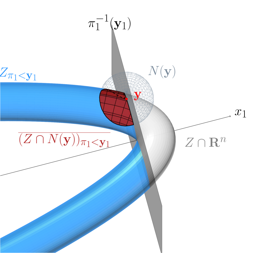
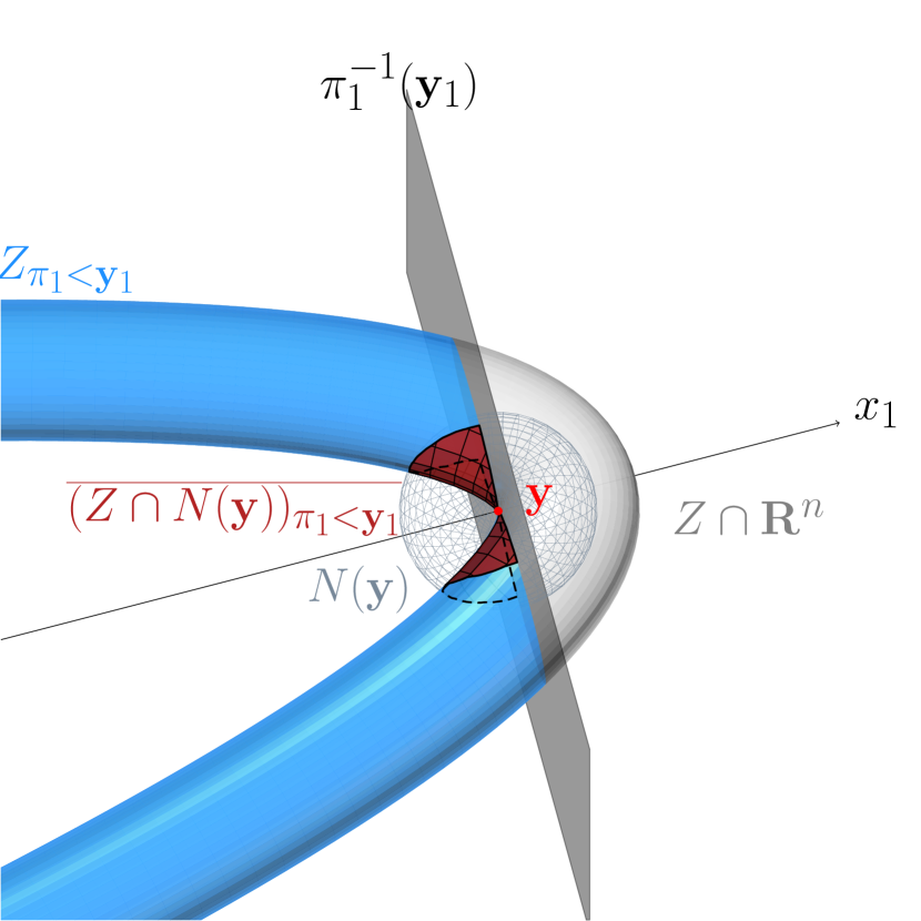
Figure 2: Illustration of Lemma 3.3 where $\bm{\varphi}=\pi_{1}$, $u={\bm{y}}_{1}$ and $Z$ is isomorphic to $\bm{V}(x_{1}^{2}+x_{2}^{2}-1)\times{\color[rgb]{0,0,0}\bm{V}(x_{1}+x_{2}^{2})}$. On the left, ${\bm{y}}$ is not critical and one sees that it satisfies all the statements. On the right ${\bm{y}}$ is critical, and $(Z\cap N({\bm{y}}))_{\mid\pi_{1}<{\bm{y}}_{1}}$ is disconnected. Note that in both cases, ${\bm{y}}_{1}$ is a critical value.

Proof.

Let $\bm{\alpha},N^{\prime},N$ and ${\bm{f}}$ be obtained by applying Lemma 3.2. Let ${\bm{F}}\colon{\bm{z}}^{\prime}\in N^{\prime}\mapsto\left({\bm{z}}^{\prime},{\bm{f}}({\bm{z}}^{\prime})\right)\in N$. Let $\varepsilon>0$ be such that

$$\pazocal{B}=\mathscr{B}\left(\pi_{d}(\alpha({\bm{y}})),\varepsilon\right)\subset N^{\prime}\subset\mathbf{R}^{d}$$

where $\mathscr{B}\left(\pi_{d}(\alpha({\bm{y}})),\varepsilon\right)$ is the open ball of $\mathbf{R}^{d}$ with radius $\varepsilon$ and center $\pi_{d}(\alpha({\bm{y}}))$. We claim that taking $N({\bm{y}})=\bm{\alpha}^{-1}({\bm{F}}(\pazocal{B}))$ is enough to prove the result.

First, ${\bm{F}}(\pazocal{B})$ is open, semi-algebraic and semi-algebraically connected, since ${\bm{F}}$ is an open continuous map on $\pazocal{B}$. Then, by assumptions on $\bm{\alpha}$, together with Lemma 2.1, $\bm{\alpha}^{-1}({\bm{F}}(\pazocal{B}))$ is a semi-algebraically connected open neighborhood of ${\bm{y}}$. Hence $N({\bm{y}})$ satisfies statement $a)$.

Besides, remark that ${\bm{F}}(\pazocal{B})\subset\bm{\alpha}(Z)$, so that

$$(\bm{\alpha}(Z)\cap{\bm{F}}(\pazocal{B}))_{\mid\pi_{1}<u}={\bm{F}}(\pazocal{B})_{\mid\pi_{1}<u}={\bm{F}}(\pazocal{B}_{\mid\pi_{1}<u})$$

as $\pi_{1}({\bm{F}}({\bm{z}}^{\prime}))=\pi_{1}({\bm{z}}^{\prime})$ for ${\bm{z}}^{\prime}\in N^{\prime}$. Since $\pi_{1}(\alpha({\bm{y}}))=\bm{\varphi}({\bm{y}})=u$, the semi-algebraic set $\pazocal{B}_{\mid\pi_{1}<u}$ is non-empty and semi-algebraically connected (since $\pazocal{B}$ is convex), and so is its image through ${\bm{F}}$ by [4, Section 3.2]. But remark that for all $X\subset\mathbf{R}$,

$$(Z\cap N({\bm{y}}))_{\mid\bm{\varphi}\in X}=\bm{\alpha}^{-1}\left((\bm{\alpha}(Z)\cap{\bm{F}}(\pazocal{B}))_{\mid\pi_{1}\in X}\right)=\alpha^{-1}\circ{\bm{F}}(\pazocal{B}_{\mid\pi_{1}\in X}),$$ (3)

since $\bm{\varphi}\circ\bm{\alpha}^{-1}=\pi_{1}$. Therefore, by Lemma 2.1, $(Z\cap N({\bm{y}}))_{\mid\bm{\varphi}<u}$ is non-empty and semi-algebraically connected, as claimed in statement $b)$.

To prove assertion $c)$, remark that $\pazocal{B}_{\mid\pi_{1}=u}$ is contained in $\overline{\pazocal{B}_{\mid\pi_{1}<u}}$, so that $\alpha^{-1}\circ{\bm{F}}(\pazocal{B}_{\mid\pi_{1}=u})$ is contained in $\alpha^{-1}\circ{\bm{F}}(\overline{\pazocal{B}_{\mid\pi_{1}<u}})$. Since ${\bm{F}}$ and $\alpha^{-1}$ are continuous,

$$\alpha^{-1}\circ{\bm{F}}\left(\overline{\pazocal{B}_{\mid\pi_{1}<u}}\right)\subset\overline{\alpha^{-1}\circ{\bm{F}}\left(\pazocal{B}_{\mid\pi_{1}<u}\right)}.$$

Finally, by (3), we get

$$(Z\cap N({\bm{y}}))_{\mid\bm{\varphi}=u}\subset\overline{(Z\cap N({\bm{y}})_{\mid\bm{\varphi}<u}}.$$

∎

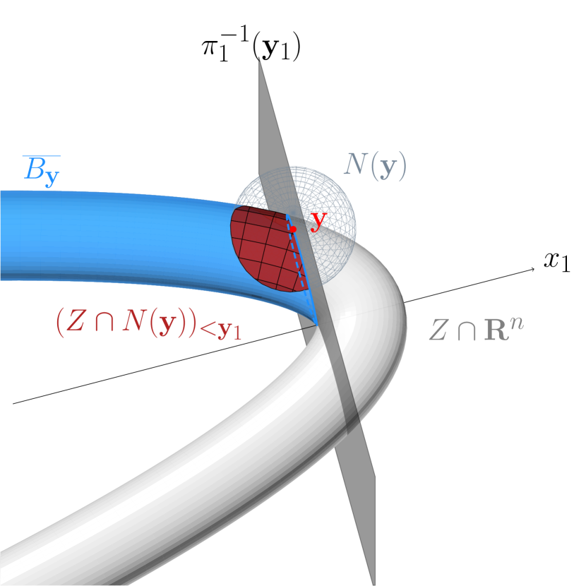
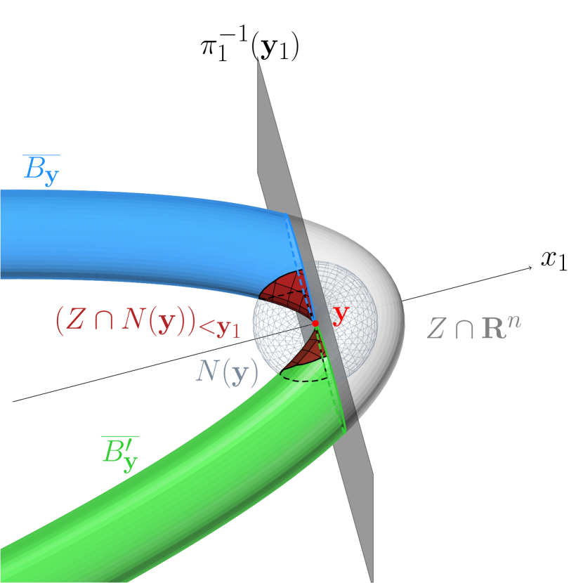
Figure 3: Illustration of Lemma 3.4 where $\bm{\varphi}=\pi_{1}$, $u={\bm{y}}_{1}$ and $Z$ is isomorphic to $\bm{V}(x_{1}^{2}+x_{2}^{2}-1)\times{\color[rgb]{0,0,0}\bm{V}(x_{1}+x_{2}^{2})}$. On the left ${\bm{y}}$ is not critical and one sees that ${\bm{y}}\in\overline{B_{\bm{y}}}$ and $(Z\cap N({\bm{y}}))_{\mid\pi_{1}<{\bm{y}}_{1}}\subset B_{\bm{y}}$. However on the right, ${\bm{y}}$ is critical, and one observes that ${\bm{y}}$ belongs to both $\overline{B_{\bm{y}}}$ and $\overline{B_{\bm{y}}^{\prime}}$, and, in addition, that $(Z\cap N({\bm{y}}))_{\mid\pi_{1}<{\bm{y}}_{1}}$ is not contained in any of these components. Note that in both cases, ${\bm{y}}_{1}$ is a critical value.

Lemma 3.4.

Let ${\bm{y}}$ be in $Z\cap\mathbf{R}^{n}-K(\bm{\varphi},Z)$, let $u=\bm{\varphi}({\bm{y}})$ and let $N({\bm{y}})$ as in Lemma 3.3. Then, there exists a unique semi-algebraically connected component $B_{\bm{y}}$ of $Z_{\mid\bm{\varphi}<u}$ such that ${\bm{y}}\in\overline{B_{\bm{y}}}$. Moreover,

$$(Z\cap N({\bm{y}}))_{\mid\bm{\varphi}<u}\subset B_{\bm{y}}.$$

This lemma is illustrated in Figure 3.

Proof.

By the second item of Lemma 3.3, $(Z\cap N({\bm{y}}))_{\mid\bm{\varphi}<u}$ is non-empty and semi-algebraically connected. Thus, it is contained in a semi-algebraically connected component $B_{\bm{y}}$ of $Z_{\mid\bm{\varphi}<u}$. Since the semi-algebraically connected components of $Z_{\mid\bm{\varphi}<u}$ are pairwise disjoint, $B_{\bm{y}}$ is well defined and unique. Moreover by Lemma 3.3,

$${\bm{y}}\in\overline{(Z\cap N({\bm{y}}))_{\mid\bm{\varphi}<u}}\subset\overline{B_{\bm{y}}}.$$

Finally, suppose that there exists another connected component $B^{\prime}$ of $Z_{\mid\bm{\varphi}<u}$ such that ${\bm{y}}\in\overline{B^{\prime}}$. Then ${\bm{y}}$ belongs to the closure of $B^{\prime}$, so that $N({\bm{y}})\cap B^{\prime}\neq\emptyset$, since $N({\bm{y}})$ is a neighborhood of ${\bm{y}}$. Thus $B^{\prime}\cap B_{\bm{y}}$ is not empty, and since they are both semi-algebraically connected components of the same set, $B^{\prime}=B_{\bm{y}}$. ∎

Let us see a geometric consequence of this result. The following lemma shows that if $u$ is the least element of $\mathbf{R}$ such that the hypersurface $\bm{\varphi}^{-1}(\{u\})$ intersects a semi-algebraically connected component $C$ of $Z\cap\mathbf{R}^{n}$, then this intersection consists entirely of singular points of $\bm{\varphi}$ on $Z$. It is illustrated by Figure 4.

Lemma 3.5.

Let ${\bm{y}}\in Z\cap\mathbf{R}^{n}$ with $u=\bm{\varphi}({\bm{y}})$ and let $C$ be the semi-algebraically connected component of $Z_{\mid\bm{\varphi}\leq u}$ containing ${\bm{y}}$. If $C_{\mid\bm{\varphi}<u}=\emptyset$ then $C=C_{\mid\bm{\varphi}=u}\subset K(\bm{\varphi},Z)$. In particular, ${\bm{y}}\in K(\bm{\varphi},Z)$.

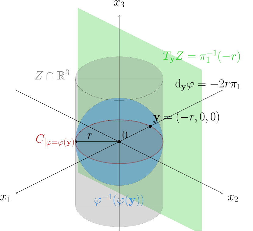
Figure 4: Illustration of Lemma 3.5 in two cases. On the left, $\bm{\varphi}=\pi_{1}$ and $Z\cap\mathbb{R}^{3}$ is a torus. The plane $\{x_{1}=u\}$ indicated satisfies $C_{\mid\bm{\varphi}<u}=\emptyset$. One sees that $C_{\mid\bm{\varphi}=u}\subset K(\bm{\varphi},Z)$, and indeed $C_{\mid\bm{\varphi}=u}=\{{\bm{y}}\}$. On the right, $\bm{\varphi}$ is the square of the Euclidean norm, and $Z$ is a cylinder of radius $r$. Remark first that $C_{\mid\bm{\varphi}<r}=\emptyset$. Moreover, for ${\bm{x}}=({\bm{x}}_{1},{\bm{x}}_{2},0)\in Z$, the differential at ${\bm{x}}$ of restriction of $\varphi$ to $Z$ is the restriction of the projection on the $(x_{1},x_{2})$-plane to $T_{{\bm{x}}}Z$. Since these two latter planes are orthogonal, ${\bm{x}}$ is indeed a critical point.

Proof.

If $C_{\mid\bm{\varphi}<u}=\emptyset$, since $C\subset Z_{\mid\bm{\varphi}\leq u}$ then $C=C_{\mid\bm{\varphi}=u}$ holds. Let us prove the contrapositive of the rest of the lemma. Suppose that $C_{\mid\bm{\varphi}=u}\not\subset K(\bm{\varphi},Z)$, and let

$${\bm{z}}\in C_{\mid\bm{\varphi}=u}-K(\bm{\varphi},Z).$$

Let $B_{{\bm{z}}}$ be the semi-algebraically connected component of $Z_{\mid\bm{\varphi}<u}$ obtained by applying Lemma 3.4. Since $\overline{B_{{\bm{z}}}}$ contains ${\bm{z}}$ and is a semi-algebraically connected set of $Z_{\mid\bm{\varphi}\leq u}$, $\overline{B_{{\bm{z}}}}\subset C$. Hence $C_{\mid\bm{\varphi}<u}$ contains $(\overline{B_{{\bm{z}}}})_{\mid\bm{\varphi}<u}=B_{{\bm{z}}}$, which is then not empty. ∎

We prove now an important consequence of the previous lemma. It is a fundamental property of generalized polar varieties and motivates their introduction among the ingredients of a roadmap.

Proposition 3.6.

Let $u\in\mathbf{R}$ and let $B$ be a bounded semi-algebraically connected component of $Z_{\mid\bm{\varphi}<u}$. Then $B\cap K(\bm{\varphi},Z)\neq\emptyset$.

Proof.

Since $\bm{\varphi}$ is a semi-algebraic continuous map and $B$ is semi-algebraic, then $\bm{\varphi}(\overline{B})$ is a closed and bounded semi-algebraic set by [4, Theorem 3.23]. In particular, $\bm{\varphi}$ reaches its minimum $\bm{\varphi}({\bm{z}})$ on $\overline{B}$ and since $\emptyset\neq B\subset Z_{\mid\bm{\varphi}<u}$,then $\bm{\varphi}({\bm{z}})<u$. But $B$ is a semi-algebraically connected component of $Z_{\mid\bm{\varphi}<u}$, so in particular it is closed in $Z_{\mid\bm{\varphi}<u}$, so that

$$\overline{B}-B\subset Z_{\mid\bm{\varphi}=u}.$$

Therefore ${\bm{z}}\in B$ and as $B_{\mid\bm{\varphi}<\bm{\varphi}({\bm{z}})}$ is empty (${\bm{z}}$ is a minimizer), $B_{\mid\bm{\varphi}=\bm{\varphi}({\bm{z}})}$ and ${\bm{z}}$ is in $K(\bm{\varphi},Z)$ by Lemma 3.5. Finally ${\bm{z}}\in B\cap K(\bm{\varphi},Z)$, and the latter is non-empty. ∎

We are now able to prove a weaker version of Proposition 3.1, which is illustrated in Figure 5. It deals with the particular case when the map has values in some fiber $Z_{\mid\bm{\varphi}=u}$, where $u\in\mathbf{R}$.

Lemma 3.7.

Let $u\in\mathbf{R}$ and $A\subset\mathbf{R}^{k}$ be a semi-algebraically connected set. Let

$$\gamma\colon A\longrightarrow Z_{\mid\bm{\varphi}=u}-K(\bm{\varphi},Z)$$

be a continuous semi-algebraic map. Then there exists a unique semi-algebraically connected component $B$ of $Z_{\mid\bm{\varphi}<u}$ such that $\gamma(A)\subset\overline{B}$.

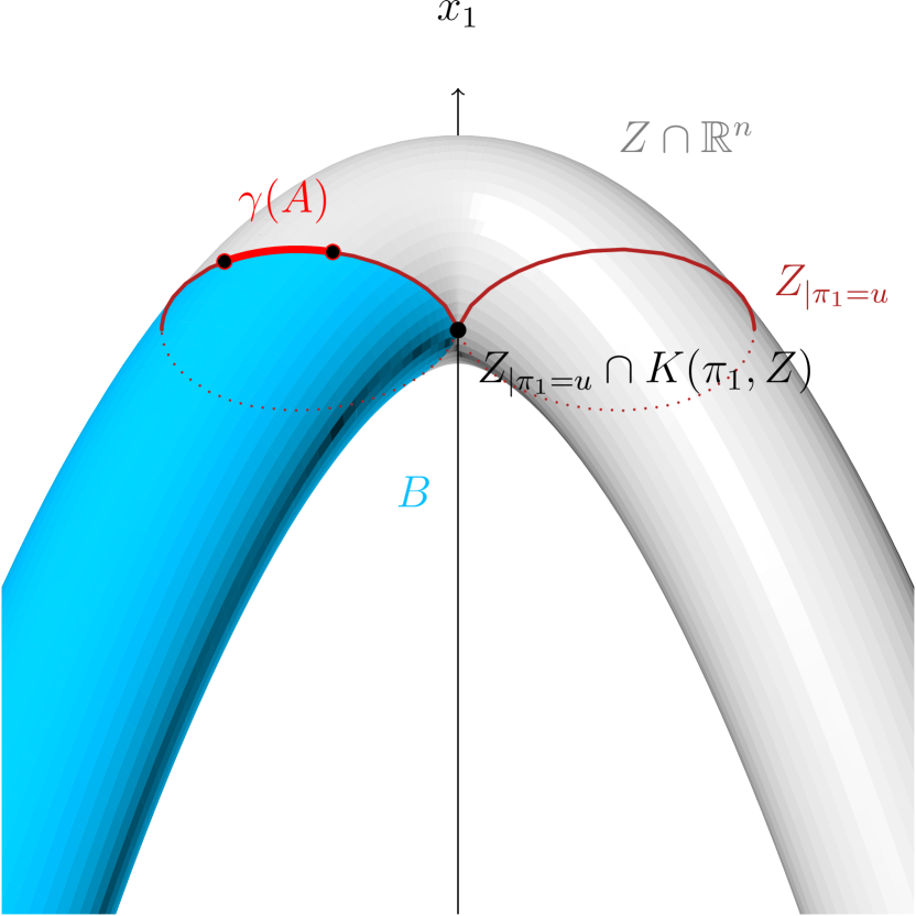
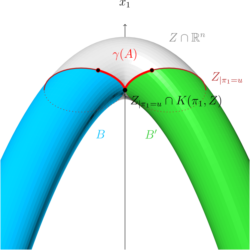
Figure 5: Illustration of the proof of Proposition 3.1 where $\bm{\varphi}=\pi_{1}$ and $Z$ is isomorphic to $\bm{V}(x_{1}^{2}+x_{2}^{2}-1)\times{\color[rgb]{0,0,0}\bm{V}(x_{1}+x_{2}^{2})}$ in two cases. On the left the $\gamma(A)\cap(Z_{\mid\pi_{1}=u}\cap K(\pi_{1},Z))=\emptyset$ and on the right, this intersection is non-empty.

Proof.

Let $\bm{a}_{0}\in A$ and ${\bm{y}}=\gamma(\bm{a}_{0})$, by assumption, ${\bm{y}}\in Z_{\mid\bm{\varphi}=u}-K(\bm{\varphi},Z)$. Then by Lemmas 3.3 and 3.4, there exist an open neighborhood $N({\bm{y}})$ of ${\bm{y}}$ and a semi-algebraically connected component $B_{\bm{y}}$ of $Z_{\mid\bm{\varphi}<u}$ such that

$$(Z\cap N({\bm{y}}))_{\mid\bm{\varphi}=u}\subset\overline{(Z\cap N({\bm{y}}))_{\mid\bm{\varphi}<u}}\subset\overline{B_{{\bm{y}}}}.$$

Hence for every ${\bm{z}}\in(Z\cap N({\bm{y}}))_{\mid\bm{\varphi}=u}-K(\bm{\varphi},Z)$, ${\bm{z}}\in\overline{B_{{\bm{y}}}}$ so that $B_{{\bm{z}}}=B_{{\bm{y}}}$ by application of Lemma 3.4. Since $\gamma$ is a continuous semi-algebraic map, there exists an open semi-algebraic neighborhood $N^{\prime}(\bm{a}_{0})$ of $\bm{a}_{0}$ such that

$$\gamma(N^{\prime}(\bm{a}_{0}))\subset(Z\cap N({\bm{y}}))_{\mid\bm{\varphi}=u}-K(\bm{\varphi},Z).$$

Hence the map $\bm{a}\mapsto B_{\gamma(\bm{a})}$ is constant on $N(\bm{a}_{0})$. Let

$$\mathfrak{B}:\bm{a}\in A\mapsto B_{\gamma(\bm{a})}\in\pazocal{P}(Z_{\mid\bm{\varphi}<u})$$

be the map given by Lemma 3.4, where $\pazocal{P}(Z_{\mid\bm{\varphi}<u})$ denote the power set of $Z_{\mid\bm{\varphi}<u}$. We proved that $\mathfrak{B}$ is locally constant on $A$ and then, equivalently, continuous for the discrete topology on $\pazocal{P}(Z_{\mid\bm{\varphi}<u})$. But since $A$ is semi-algebraically connected, $\mathfrak{B}(A)$ is connected for the discrete topology, that is $\mathfrak{B}$ is constant $A$.

Let then $B$ be the constant value that $\mathfrak{B}$ takes on $A$. By Lemma 3.4, for all $\bm{a}\in A$, $\gamma(\bm{a})\in\overline{B_{\gamma(\bm{a})}}=\overline{B}$, that is $\gamma(A)\subset\overline{B}$. Besides, if $B^{\prime}$ is another semi-algebraically connected component of $Z_{\mid\bm{\varphi}<u}$ such that $\gamma(A)\subset\overline{B^{\prime}}$, then for all $\bm{a}\in A$,

$$\gamma(\bm{a})\in\overline{B}\cap\overline{B^{\prime}}\cap Z_{\mid\bm{\varphi}=u}-K(\bm{\varphi},Z),$$

so that $B=B^{\prime}$ by uniqueness in Lemma 3.4. ∎

We can now prove the main proposition by sticking together all the pieces. The points of the map that belong to the fiber $Z_{\mid\bm{\varphi}=u}$ are managed by Lemma 3.7, while the remaining ones, in $Z_{\mid\bm{\varphi}<u}$, are more convenient to deal with. This proof is illustrated by Figure 6.

Proof of Proposition 3.1.

Since $\gamma$ is semi-algebraic and continuous, $\gamma(A)$ is semi-algebraically connected. Hence, if $\gamma(A)\subset Z_{\mid\bm{\varphi}<u}$, it is contained in a unique semi-algebraically connected component $B$ of $Z_{\mid\bm{\varphi}<u}$ and we are done.

We assume now that $\gamma(A)\not\subset Z_{\mid\bm{\varphi}<u}$. Let $G=\gamma^{-1}(Z_{\mid\bm{\varphi}=u})$. It is a closed subset of $A$ since $Z_{\mid\bm{\varphi}=u}$ is closed in $Z_{\mid\bm{\varphi}\leq u}$ and $\gamma$ is continuous. Then, let $G_{1},\dotsc,G_{N}$ be the semi-algebraically connected components of $G$; they are closed in $A$ since they are closed in $G$, which is closed in $A$. Besides, let $H_{1},\dotsc,H_{M}$ be the semi-algebraically connected components of $A-G$. They are open in $A$ since they are open in $A-G$ , which is open in $A$.

We define a map $\mathfrak{B}\colon A\to\pazocal{P}(Z_{\mid\bm{\varphi}<u})$, where $\pazocal{P}(Z_{\mid\bm{\varphi}<u})$ is the power set of $Z_{\mid\bm{\varphi}<u}$. The family formed by both $G_{1},\dotsc,G_{N}$ and $H_{1},\dotsc H_{M}$ is a partition of $A$; hence, we can define $\mathfrak{B}$ by defining it on this partition.

$\bm{H_{i}:}$

Since $H_{i}\subset A-G$, $\gamma(H_{i})\subset Z_{\mid\bm{\varphi}<u}$ and $\gamma(H_{i})$ is semi-algebraically connected as $\gamma$ is continuous. Then, there exists a unique semi-algebraically connected component $B_{i}$ of $Z_{\mid\bm{\varphi}<u}$ such that $\gamma(H_{i})\subset B_{i}\subset\overline{B_{i}}$.

$\bm{G_{i}:}$

Since $G_{i}$ is semi-algebraically connected and $\gamma(G_{i})\subset Z_{\mid\bm{\varphi}=u}-K(\bm{\varphi},Z)$, Lemma 3.7 with $A=G_{i}$ states that there is a unique semi-algebraically connected component $B^{\prime}_{i}$ of $Z_{\mid\bm{\varphi}<u}$ such that $\gamma(G_{i})\subset\overline{B^{\prime}_{i}}$.

Therefore, for all $\bm{a}\in A$, let $\mathfrak{B}$ such that

$$\mathfrak{B}(\bm{a})=\left\{\begin{array}[]{ll}B_{i}&\text{if $\bm{a}\in H_{i}$}\\ B_{i}^{\prime}&\text{if $\bm{a}\in G_{i}$}\\ \end{array}\right.\text{so that }\gamma(\bm{a})\in\overline{\mathfrak{B}(\bm{a})}.$$

Let us show that $\mathfrak{B}$ is locally constant, that is, for every $\bm{a}\in A$, there exists an open Euclidean neighborhood $N(\bm{a})\subset A$ of $\bm{a}$, such that for all $\bm{a}^{\prime}\in N(\bm{a})$, $\mathfrak{B}(\bm{a}^{\prime})=\mathfrak{B}(\bm{a})$. Then, we will conclude by connectedness as above. Let $\bm{a}\in A$ and $1\leq i\leq\max(M,N)$.

• If $\bm{a}\in H_{i}$, since $H_{i}$ is open in $A$, there exists an open Euclidean neighborhood $N(\bm{a})$ of $\bm{a}$ contained in $H_{i}$. By construction, for all $\bm{a}^{\prime}\in N(\bm{a})$, $\mathfrak{B}(\bm{a}^{\prime})=\mathfrak{B}(\bm{a})$. Moreover, since $H_{i}$ is semi-algebraically connected, this also proves that $\mathfrak{B}$ is actually constant on $H_{i}$, and we let $\mathfrak{B}(H_{i})$ be the unique value it assumes on $H_{i}$.

• Else $\bm{a}\in G_{i}$, since the $G_{j}$’s are closed in $A$, then $\bm{a}$ does not belong to the closure of any other $G_{j}$, $j\neq i$. However, the set

  $$J=\left\{1\leq j\leq M\mid\bm{a}\in\overline{H_{j}}\right\}$$

  is not empty. By construction, $\gamma(\bm{a})\in\overline{\mathfrak{B}(\bm{a})}$ and by definition of $J$, for every $j\in J$, $\gamma(\bm{a})\in\overline{\mathfrak{B}(H_{j})}$. But, by Lemma 3.4 applied with ${\bm{y}}=\gamma(\bm{a})$, such a semi-algebraically connected component is unique. Hence for all $j\in J$, $\mathfrak{B}(H_{j})=\mathfrak{B}(\bm{a})$. One can then take $N(\bm{a})=\mathscr{B}(\bm{a},r)$ with $r>0$ such that this open ball intersects either the $H_{j}$’s for $j\in J$ or $G_{i}$, and only them.

Finally, we proved that $\mathfrak{B}$ is locally constant and then, equivalently, continuous for the discrete topology on $\pazocal{P}(Z_{\mid\bm{\varphi}<u})$. Since $A$ is semi-algebraically connected, $\mathfrak{B}(A)$ is connected for the discrete topology and $\mathfrak{B}$ is constant on $A$. Denoting by $B\subset Z_{\mid\bm{\varphi}<u}$ the unique value it assumes, we have $\gamma(A)\subset\overline{B}$ as claimed. Besides if $B^{\prime}$ is another semi-algebraically connected component of $Z_{\mid\bm{\varphi}<u}$ such that $\gamma(A)\subset\overline{B^{\prime}}$, then in particular $\overline{B}\cap\overline{B^{\prime}}$ contains $\gamma(G_{1})\subset Z_{\mid\bm{\varphi}=u}-K(\bm{\varphi},Z)$, so that $B=B^{\prime}$ by Lemma 3.7. ∎

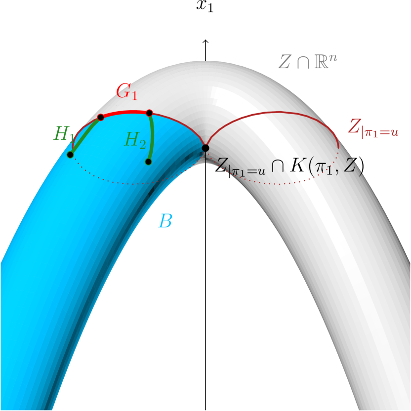
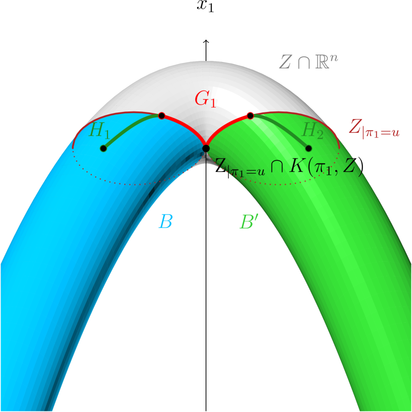
Figure 6: Illustration of the proof of Proposition 3.1 with $\bm{\varphi}=\pi_{1}$ and $Z$ is isomorphic to $\bm{V}(x_{1}^{2}+x_{2}^{2}-1)\times{\color[rgb]{0,0,0}\bm{V}(x_{1}+x_{2}^{2})}$ in two cases. The intersection $\gamma(A)\cap(Z_{\mid\pi_{1}=u}\cap K(\pi_{1},Z))$ is empty on the left while, on the right, it is not.

We then deduce the following consequence on the semi-algebraically connected components of $Z$ with respect to $\bm{\varphi}$. This result is illustrated in Figure 7.

Corollary 3.8.

Let $\bm{\varphi}\colon\mathbf{C}^{n}\rightarrow\mathbf{C}$ be a regular map defined over $\mathbf{R}$ and $Z\subset\mathbf{C}^{n}$ be an equidimensional algebraic set of positive dimension. Let $u\in\mathbf{R}$ such that $Z_{\mid\bm{\varphi}=u}\cap K(\bm{\varphi},Z)=\emptyset$ and let $C$ be a semi-algebraically connected component of $Z_{\mid\bm{\varphi}\leq u}$. Then, $C_{\mid\bm{\varphi}<u}$ is a semi-algebraically connected component of $Z_{\mid\bm{\varphi}<u}$.

Proof.

Let $\gamma$ be the inclusion map $\gamma\colon C\hookrightarrow Z_{\mid\bm{\varphi}\leq u}$. Since $Z_{\mid\bm{\varphi}=u}\cap K(\bm{\varphi},Z)=\emptyset$, $\gamma$ satisfies the assumptions of Proposition 3.1 with $A=C$. Then there exists a unique semi-algebraically connected component $B$ of $Z_{\mid\bm{\varphi}<u}$ such that $C\subset\overline{B}$, so that $C_{\mid\bm{\varphi}<u}\subset\overline{B}_{\mid\bm{\varphi}<u}=B$.

First, since $Z_{\mid\bm{\varphi}=u}\cap K(\bm{\varphi},Z)=\emptyset$ by assumption, then in particular $C_{\mid\bm{\varphi}=u}\not\subset K(\bm{\varphi},Z)$. By the contrapositive of Lemma 3.5, $C_{\mid\bm{\varphi}<u}$ is not empty. Hence, since $B$ is a semi-algebraically connected set of $Z_{\mid\bm{\varphi}\leq u}$, containing $C_{\mid\bm{\varphi}<u}$, $B$ is contained in the semi-algebraically connected component $C$ of $Z_{\mid\bm{\varphi}\leq u}$. Finally $B\subset Z_{\mid\bm{\varphi}<u}\cap C=C_{\mid\bm{\varphi}<u}$ and $C_{\mid\bm{\varphi}<u}=B$, which is a semi-algebraically connected component of $Z_{\mid\bm{\varphi}<u}$. ∎

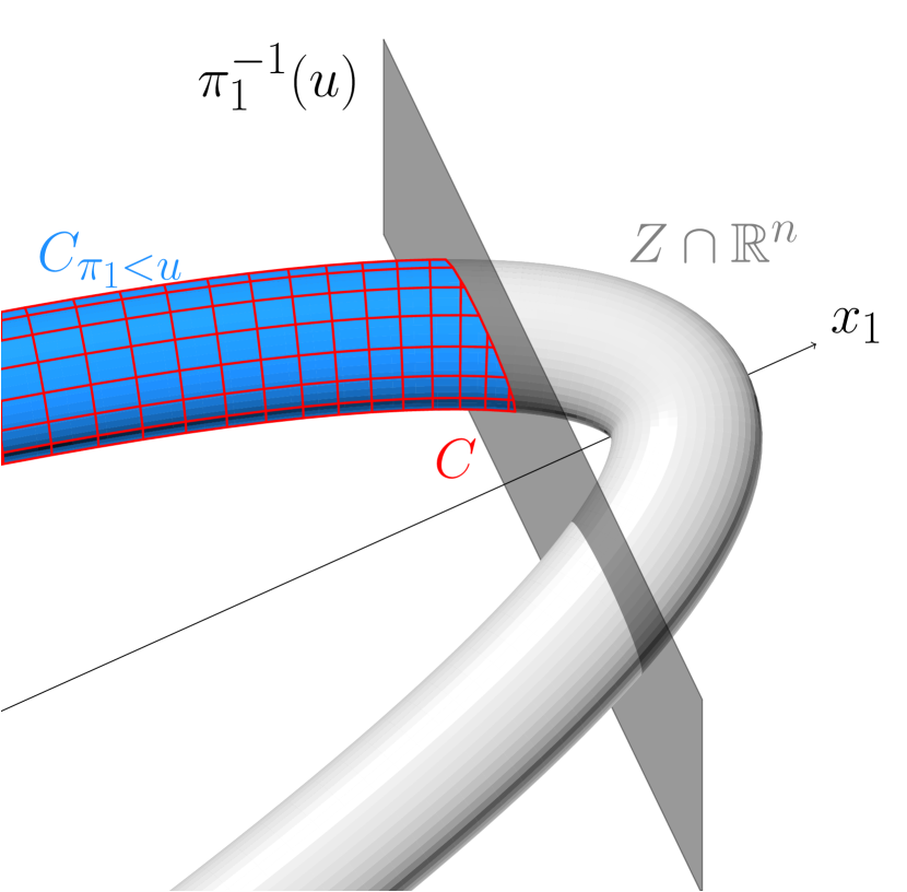
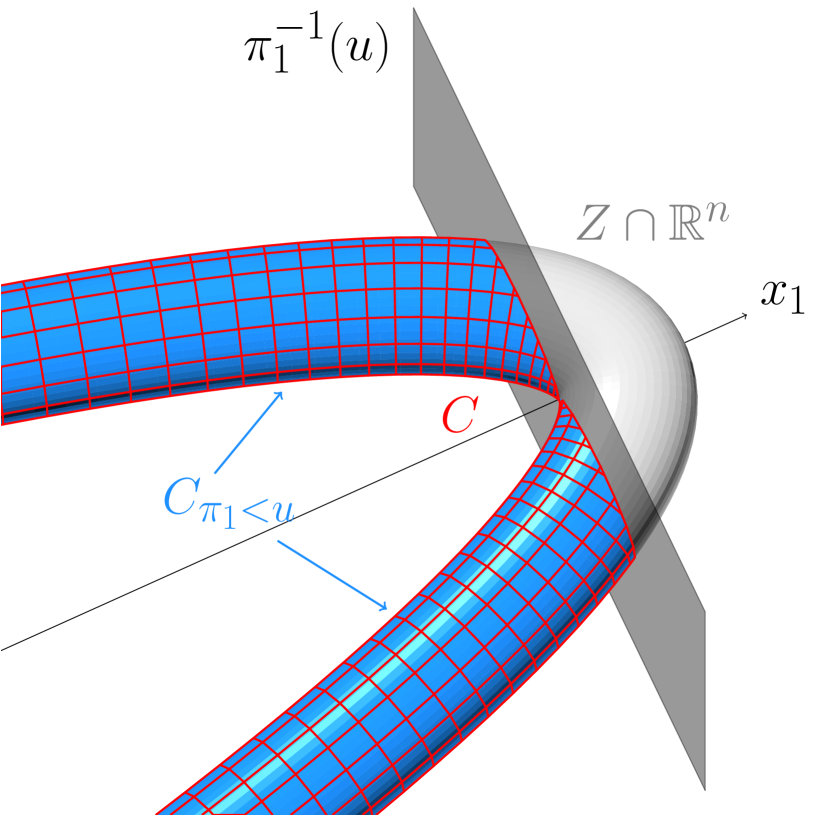
Figure 7: Illustration of Corollary 3.8 where $\bm{\varphi}=\pi_{1}$ and $Z$ is isomorphic to $\bm{V}(x_{1}^{2}+x_{2}^{2}-1)\times{\color[rgb]{0,0,0}\bm{V}(x_{1}+x_{2}^{2})}$. On the left $Z_{\mid\pi_{1}=u}\cap K(\pi_{1},Z)=\emptyset$ and one sees that $C_{\mid\pi_{1}<u}$ is still a semi-algebraically connected component of $Z_{\mid\pi_{1}<u}$. On the right $Z_{\mid\pi_{1}=u}\cap K(\pi_{1},Z)\neq\emptyset$ and one sees that $C_{\mid\pi_{1}<u}$ is disconnected.

3.2 Fibration and critical values

As in [23, Section 3.2] we are going to use a Nash version of Thom’s isotopy lemma, stated in [16], which, again, is an ingredient of Morse theory. We refer to [4, Section 3.5] for the definitions of Nash diffeomorphisms, manifolds and submersions together with their properties.

Proposition 3.9.

Let $\bm{\varphi}\colon\mathbf{C}^{n}\rightarrow\mathbf{C}$ be a regular map defined over $\mathbf{R}$ and $A\subset\bm{\varphi}^{-1}((-\infty,w))\cap\mathbf{R}^{n}$ be a semi-algebraically connected semi-algebraic set. Let $v<w$ such that $A_{\mid\bm{\varphi}\in(v,w)}$ is a non-empty Nash manifold, bounded, closed in $\bm{\varphi}^{-1}((v,w))\cap\mathbf{R}^{n}$ and such that $\bm{\varphi}$ is a submersion on $A_{\mid\bm{\varphi}\in(v,w)}$. Then for all $u\in[v,w)$, $A_{\mid\bm{\varphi}\leq u}$ is non-empty and semi-algebraically connected.

Proof.

We first prove that $\bm{\varphi}\colon A_{\mid\bm{\varphi}\in(v,w)}\rightarrow(v,w)$ is a proper surjective submersion. Since $A_{\mid\bm{\varphi}\in(v,w)}$ is bounded and $\bm{\varphi}$ is semi-algebraic and continuous, $\bm{\varphi}\colon A_{\mid\bm{\varphi}\in(v,w)}\rightarrow(v,w)$ is a proper map. Let us prove that $\bm{\varphi}$ is also surjective on $A_{\mid\bm{\varphi}\in(v,w)}$ that is

$$\bm{\varphi}(A_{\mid\bm{\varphi}\in(v,w)})=(v,w).$$

By assumption, $\bm{\varphi}$ is a submersion from $A_{\mid\bm{\varphi}\in(v,w)}$ to $(v,w)$. Then by the semi-algebraic inverse function theorem [4, Proposition 3.29], $\bm{\varphi}$ is an open map. Besides, as $A_{\mid\bm{\varphi}\in(v,w)}$ is closed and bounded, there exists a closed and bounded semi-algebraic set $X\subset\mathbf{R}^{n}$ such that $A_{\mid\bm{\varphi}\in(v,w)}=X\cap\bm{\varphi}^{-1}((v,w))=X_{\mid\bm{\varphi}\in(v,w)}$. Then

$$\bm{\varphi}(A_{\mid\bm{\varphi}\in(v,w)})=\bm{\varphi}(X_{\mid\bm{\varphi}\in(v,w)})=\bm{\varphi}(X)\cap(v,w).$$

Since $X$ is bounded and closed, $\bm{\varphi}(X)$ is closed and bounded by [4, Theorem 3.23]. Hence, $\bm{\varphi}(A_{\mid\bm{\varphi}\in(v,w)})$ is both open and closed in $(v,w)$. Since $(v,w)$ is semi-algebraically connected, $\bm{\varphi}(A_{\mid\bm{\varphi}\in(v,w)})=(v,w)$.

By the Nash version of Thom’s isotopy lemma [16, Theorem 2.4], since the map $\bm{\varphi}\colon A_{\mid\bm{\varphi}\in(v,w)}\rightarrow(v,w)$ is a proper surjective submersion, it is a globally trivial fibration. Hence, for $\zeta\in(v,w)$, there exists a Nash diffeomorphism $\Psi$ of the form

$$\begin{array}[]{cccc}\Psi\colon&A_{\mid\bm{\varphi}\in(v,w)}&\longrightarrow&(v,w)\times A_{\mid\bm{\varphi}=\zeta}\\[3.00003pt] &{\bm{y}}&\longmapsto&(\;\bm{\varphi}({\bm{y}})\;\>,\;\,\psi({\bm{y}})\;\;)\end{array}.$$

We now proceed to prove the main statement of the proposition. There are, at first sight, two different situations to consider: whether $u>v$ or $u=v$ (see Figure 8). Using Puiseux series, we actually prove them simultaneously.

Take $u\in[v,w)$; we prove that $A_{\mid\bm{\varphi}\leq u}$ is non-empty and semi-algebraically connected. To prove that $A_{\mid\bm{\varphi}=u}$ is non-empty, we consider ${\bm{z}}\in A_{\mid\bm{\varphi}=\zeta}$ and the map

$$\begin{array}[]{cccc}\gamma\colon&[0,1)&\rightarrow&A_{\mid\bm{\varphi}\in(v,w)}\\[3.00003pt] &t&\mapsto&\Psi^{-1}(tu+(1-t)\zeta,{\bm{z}}).\end{array}$$

This map is well defined and continuous, since $\Psi$ is a Nash diffeomorphism from $A_{\mid\bm{\varphi}\in(v,w)}$ to $(v,w)\times A_{\mid\bm{\varphi}=\zeta}$, and satisfies $\bm{\varphi}(\gamma(t))=tu+(1-t)\zeta$ for every $t\in[0,1)$. Moreover $\gamma$ is a bounded map as $A_{\mid\bm{\varphi}\in(v,w)}$ is bounded by assumption. Then, by [4, Proposition 3.21], $\gamma$ can be continuously extended to $[0,1]$, with $\bm{\varphi}(\gamma(t))=tu+(1-t)\zeta$ continuous on $[0,1]$, and $\bm{\varphi}(\gamma(1))=u$. Finally $\gamma(1)\in A_{\mid\bm{\varphi}\leq u}$ and $A_{\mid\bm{\varphi}\leq u}$ is not empty.

We prove now that $A_{\mid\bm{\varphi}\leq u}$ is semi-algebraically connected. Consider two points ${\bm{y}}$ and ${\bm{y}}^{\prime}$ in $A_{\mid\bm{\varphi}\leq u}$. Since $A$ is semi-algebraically connected by assumption, there exists a continuous path $\gamma\colon[0,1]\rightarrow A$ such that $\gamma(0)={\bm{y}}$ and $\gamma(1)={\bm{y}}^{\prime}$. Let us construct, from $\gamma$, another path that lies in $A_{\mid\bm{\varphi}\leq u}$.

Let $\varepsilon$ be an infinitesimal, and let $\mathbf{R}^{\prime}=\mathbf{R}\langle\varepsilon\rangle$ be the field of algebraic Puiseux series in $\varepsilon$ (see [4, Section 2.6]). We denote by $A^{\prime},(v,w)^{\prime},\Psi^{\prime},\psi^{\prime},\bm{\varphi}^{\prime}$ and $\gamma^{\prime}$ the extensions of respectively $A,(v,w),\Psi,\psi,\bm{\varphi}$ and $\gamma$ to $\mathbf{R}^{\prime}$ in the sense of [4, Proposition 2.108]. According to [4, Exercise 2.110], $\Psi^{\prime}\colon A_{\mid\bm{\varphi}\in(v,w)^{\prime}}^{\prime}\rightarrow(v,w)^{\prime}\times A_{\mid\bm{\varphi}=\zeta}^{\prime}$ is a bijective map. Then let $g^{\prime}\colon[0,1]^{\prime}\subset\mathbf{R}^{\prime}\rightarrow A^{\prime}$ be such that

$$g^{\prime}(t)=\gamma^{\prime}(t) \quad\bm{\varphi}^{\prime}(\gamma^{\prime}(t))\leq u+\varepsilon,$$ if

$$g^{\prime}(t)=\Psi^{\prime-1}(u+\varepsilon,\psi^{\prime}(\gamma^{\prime}(t))) \quad u+\varepsilon\leq\bm{\varphi}^{\prime}(\gamma^{\prime}(t))<w.$$ if

This map is well defined since $u+\varepsilon\in(v,w)$ and if $\bm{\varphi}^{\prime}(\gamma^{\prime}(t))=u+\varepsilon$, then $\Psi^{\prime-1}(u+\varepsilon,\psi^{\prime}(\gamma^{\prime}(t)))=\gamma^{\prime}(t)$. Moreover $g^{\prime}$ is a continuous semi-algebraic map since by [4, Exercise 3.4], $\Psi^{\prime-1}$, $\psi^{\prime}$ and $\gamma^{\prime}$ are continuous semi-algebraic maps.

Finally one observes that $g^{\prime}$ is bounded over $\mathbf{R}$. Indeed if $\bm{\varphi}^{\prime}(\gamma^{\prime}(t))\leq u+\varepsilon$, then $g^{\prime}(t)=\gamma(t)$, which is continuous on $[0,1]^{\prime}$ and then bounded over $\mathbf{R}$. Else $\bm{\varphi}^{\prime}(\gamma^{\prime}(t))\in(v,w)$ and $g^{\prime}(t)\in A^{\prime}_{\mid\bm{\varphi}\in(v,w)^{\prime}}$, which is bounded over $\mathbf{R}$ by [4, Proposition 3.19] since $A_{\mid\bm{\varphi}\in(v,w)}$ is. Hence, its image $G^{\prime}=g^{\prime}([0,1]^{\prime})$ is a semi-algebraically connected semi-algebraic set, bounded over $\mathbf{R}$ and contained in $A^{\prime}_{\mid\bm{\varphi}\leq u+\varepsilon}$.

Let $G=\operatorname{lim_{\varepsilon}}{G^{\prime}}$. By [4, Proposition 12.49], $G$ is a closed and bounded semi-algebraic set. Then, since $\bm{\varphi}$ is a continuous semi-algebraic map defined over $G$, by [4, Lemma 3.24] for all ${\bm{z}}^{\prime}\in G^{\prime}$,

$$\bm{\varphi}(\operatorname{lim_{\varepsilon}}{\bm{z}}^{\prime})=\operatorname{lim_{\varepsilon}}\bm{\varphi}({\bm{z}}^{\prime})\leq\operatorname{lim_{\varepsilon}}{(u+\varepsilon)}=u$$

So that $G$ is contained in $A_{\mid\bm{\varphi}\leq u}$. In addition, since $G^{\prime}$ is semi-algebraically connected and bounded over $\mathbf{R}$, then by [4, Proposition 12.49], $G$ is semi-algebraically connected and contains ${\bm{y}}=\operatorname{lim_{\varepsilon}}{g(0)}$ and ${\bm{y}}^{\prime}=\operatorname{lim_{\varepsilon}}{g(1)}$. We deduce that there exists, inside $G$, a semi-algebraic path connecting ${\bm{y}}$ to ${\bm{y}}^{\prime}$ in $A_{\mid\bm{\varphi}\leq u}$, which ends the proof. ∎

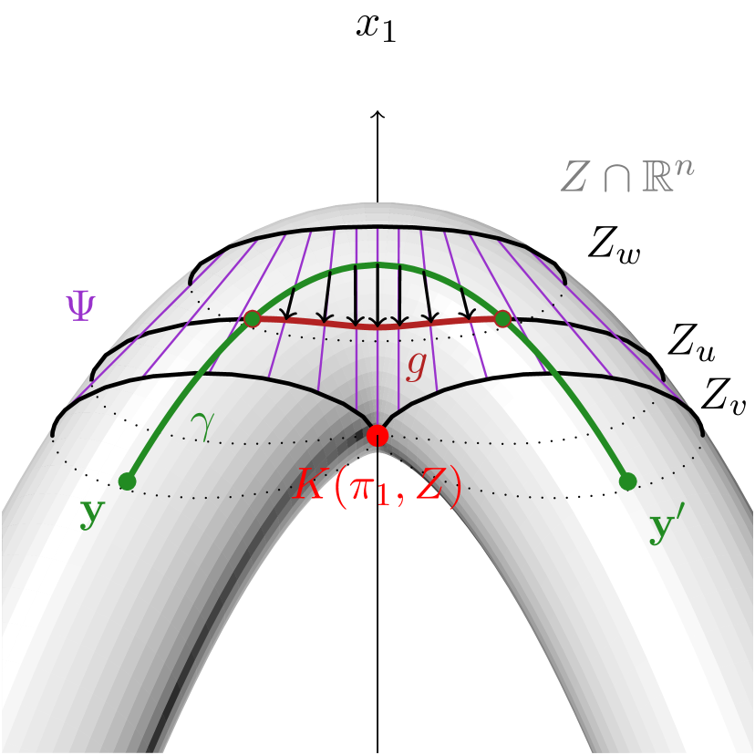
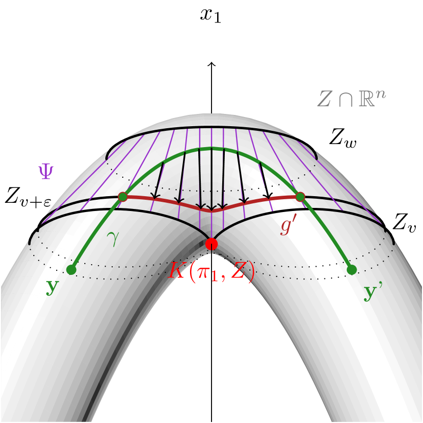
Figure 8: Illustration of the two cases covered by the proof of Proposition 3.9 where $\bm{\varphi}=\pi_{1}$ and $A=Z_{\mid\pi_{1}<w}$, where $Z$ is isomorphic to $\bm{V}(x_{1}^{2}+x_{2}^{2}-1)\times{\color[rgb]{0,0,0}\bm{V}(x_{1}+x_{2}^{2})}$. The two cases are quite similar; we consider here the one where $v$ is a critical value. One sees that $\Psi$ connects all the slices $A_{\mid\pi_{1}=u}$ for $u\in(v,w)^{\prime}$. This diffeomorphism allows to transform the problematic parts (not in $A_{\mid\pi_{1}\leq u}$) of the initial path $\gamma$ (in green), into another path $g$ (in red), that lies in $A_{\mid\pi_{1}=u}\subset A_{\mid\pi_{1}\leq u}$.

The following result is a consequence of Proposition 3.9 as it deals with a particular case. An illustration of this statement can be found in Figure 9.

Corollary 3.10.

Let $Z\subset\mathbf{C}^{n}$ be an equidimensional algebraic set of positive dimension and let $\bm{\varphi}\colon\mathbf{C}^{n}\rightarrow\mathbf{C}$ be a regular map defined over $\mathbf{R}$ and proper on $Z\cap\mathbf{R}^{n}$. Let $v<w$ be in $\mathbf{R}$ such that $Z_{\mid\bm{\varphi}\in(v,w]}\cap K(\bm{\varphi},Z)=\emptyset$, and let $C$ be a semi-algebraically connected component of $Z_{\mid\bm{\varphi}\leq w}$. Then, $C_{\mid\bm{\varphi}\leq v}$ is a semi-algebraically connected component of $Z_{\mid\bm{\varphi}\leq v}$.

Proof.

As $C_{\mid\bm{\varphi}<w}=C\cap\bm{\varphi}^{-1}((-\infty,w))\cap\mathbf{R}^{n}$, we are going to use Proposition 3.1 with $A=C_{\mid\bm{\varphi}<w}$.

First we need to prove that $C_{\mid\bm{\varphi}<w}$ is a non-empty semi-algebraically connected semi-algebraic set. Since $Z_{\mid\bm{\varphi}=w}\cap K(\bm{\varphi},Z)=\emptyset$, by Corollary 3.8 $C_{\mid\bm{\varphi}<w}$ is a semi-algebraically connected component of $Z_{\mid\bm{\varphi}<w}$. Hence it is non-empty and semi-algebraically connected.

Then, we need to prove that $C_{\mid\bm{\varphi}\in(v,w)}$ is a non-empty Nash manifold, bounded and closed in $\bm{\varphi}^{-1}((v,w))\cap\mathbf{R}^{n}$. Suppose first that $C_{\mid\bm{\varphi}\in(v,w)}=\emptyset$. Then

$$C_{\mid\bm{\varphi}\leq v}\cup C_{\mid\bm{\varphi}=w}=C\quad\text{and}\quad C_{\mid\bm{\varphi}\leq v}\cap C_{\mid\bm{\varphi}=w}=\emptyset.$$

Since $C$ is semi-algebraically connected, either $C_{\mid\bm{\varphi}\leq v}$ or $C_{\mid\bm{\varphi}=w}$ is empty (as they are both closed in $C$). In both cases our conclusion follows. It remains to tackle the case where $C_{\mid\bm{\varphi}\in(v,w)}$ is not empty, which we assume to hold from now on.

We prove that $C_{\mid\bm{\varphi}\in(v,w)}$ is bounded. Observe that $C_{\mid\bm{\varphi}\in(v,w)}\subset C_{\mid\bm{\varphi}\in[v,w]}=C\cap\mathbf{R}^{n}\cap\bm{\varphi}^{-1}([v,w])$. Recall that $\bm{\varphi}$ is proper on $Z\cap\mathbf{R}^{n}$ by assumption, and thus on $C\cap\mathbf{R}^{n}$. Hence, $C_{\mid\bm{\varphi}\in[v,w]}$ is bounded. Besides $C_{\mid\bm{\varphi}\in(v,w)}$ is closed in $\bm{\varphi}^{-1}((v,w))\cap\mathbf{R}^{n}$ as

$$C_{\mid\bm{\varphi}\in(v,w)}=C\cap\bm{\varphi}^{-1}((v,w))\cap\mathbf{R}^{n},$$

and $C$ is closed in $\mathbf{R}^{n}$ as it is closed in the closed set $Z_{\mid\bm{\varphi}\leq w}$. Since $C_{\mid\bm{\varphi}\in(v,w)}\cap K(\bm{\varphi},Z)=\emptyset$ then by [7, Proposition 3.3.11], $C_{\mid\bm{\varphi}\in(v,w)}$ is a Nash manifold of dimension $\dim(Z)$.

To apply Proposition 3.1, it remains to prove that $\bm{\varphi}$ is a Nash submersion on $C_{\mid\bm{\varphi}\in(v,w)}$. Let ${\bm{y}}\in C_{\mid\bm{\varphi}\in(v,w)}$. Since ${\bm{y}}\notin\operatorname{sing}(Z)$, then $T_{\bm{y}}C_{\mid\bm{\varphi}\in(v,w)}=T_{\bm{y}}Z\cap\mathbf{R}^{n}$ according to [7, Proposition 3.3.11]. Since $C_{\mid\bm{\varphi}\in(v,w)}\cap K(\bm{\varphi},Z)=\emptyset$, $d_{\bm{y}}\bm{\varphi}$ is onto on $T_{\bm{y}}Z$ and since $\dim{Z}>0$, the image $d_{\bm{y}}\bm{\varphi}(T_{\bm{y}}Z)$ is $\mathbf{C}$. Hence

$$d_{\bm{y}}\bm{\varphi}(T_{{\bm{y}}}C_{\mid\bm{\varphi}\in(v,w)})=\mathbf{R}.$$

We just established that all the assumptions of Proposition 3.9 are satisfied. One can then apply it to $C_{\mid\bm{\varphi}<w}$ and conclude that $C_{\mid\bm{\varphi}\leq v}$ is non-empty and semi-algebraically connected. Finally, since $C$ is a semi-algebraically connected component of $Z_{\mid\bm{\varphi}\leq w}$, any semi-algebraically connected component of $Z_{\mid\bm{\varphi}\leq v}$ contained in $C$ is contained in $C_{\mid\bm{\varphi}\leq v}$. Thus $C_{\mid\bm{\varphi}\leq v}$ is a semi-algebraically connected component of $Z_{\mid\bm{\varphi}\leq v}$. ∎

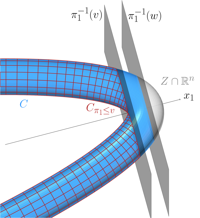
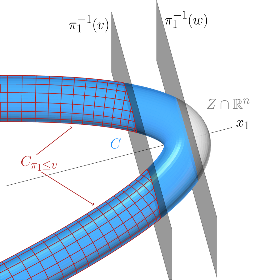
Figure 9: Illustration of Corollary 3.10 where $\bm{\varphi}=\pi_{1}$ and $Z$ is isomorphic to $\bm{V}(x_{1}^{2}+x_{2}^{2}-1)\times{\color[rgb]{0,0,0}\bm{V}(x_{1}+x_{2}^{2})}$ in two cases. On the left $Z_{\mid\pi_{1}\in(v,w)}\cap K(\pi_{1},Z)=\emptyset$ and we see that $C_{\mid\pi_{1}\leq v}$ is still a semi-algebraically connected component of $Z_{\mid\pi_{1}\leq v}$. On the right $Z_{\mid\pi_{1}\in(v,w)}\cap K(\pi_{1},Z)$ contains a point and we see that $C_{\mid\pi_{1}\leq v}$ is semi-algebraically disconnected.

4 Proof of the main connectivity result

Recall that $\bm{\varphi}=(\varphi_{1},\ldots,\varphi_{n})\subset\mathbf{R}[x_{1},\dotsc,x_{n}]$ and for $1\leq i\leq n,\bm{\varphi}_{i}\colon{\bm{y}}\mapsto(\varphi_{1}({\bm{y}}),\ldots,\varphi_{i}({\bm{y}}))$. We denote by $W_{i}=W(\bm{\varphi}_{i},V)$ the Zariski closure of the set of critical points of the restriction of $\bm{\varphi}_{i}$ to $V$ and recall that

$$K_{i}=W(\bm{\varphi}_{1},V)\cup{\color[rgb]{0,0,0}S_{i}}\cup\operatorname{sing}(V)\quad\quad\text{and}\quad\quad F_{i}=\bm{\varphi}_{i-1}^{-1}(\bm{\varphi}_{i-1}(K_{i}))\cap V,$$

where ${\color[rgb]{0,0,0}S_{i}}$ is a given subset of $V$. We suppose that the following assumptions hold:

$(\mathsf{A})$

$V$ is $d$-equidimensional and its singular locus $\operatorname{sing}(V)$ is finite;

$(\mathsf{P})$

the restriction of the map $\bm{\varphi}_{1}$ to $V\cap\mathbf{R}^{n}$ is proper and bounded from below;

$(\mathsf{B}_{1})$

$W_{i}$ is either empty or $(i-1)$-equidimensional and smooth outside $\operatorname{sing}(V)$;

$(\mathsf{B}_{2})$

for any ${\bm{y}}=({\bm{y}}_{1},\ldots,{\bm{y}}_{i})\in\mathbf{C}^{i}$, $V\cap\bm{\varphi}_{i-1}^{-1}({\bm{y}})$ is either empty or $(d-i+1)$-equidimensional;

$(\mathsf{C}_{1})$

${\color[rgb]{0,0,0}S_{i}}$ is finite;

$(\mathsf{C}_{2})$

${\color[rgb]{0,0,0}S_{i}}$ has a non-empty intersection with every semi-algebraically connected component of $W(\bm{\varphi}_{1},W_{i})\cap\mathbf{R}^{n}$.

Then the goal of this section is to prove that $W_{i}\cup F_{i}$ intersects each semi-algebraically connected component of $V\cap\mathbf{R}^{n}$ and that their intersection is semi-algebraically connected.

Let $\mathscr{R}=F_{i}\cup W_{i}$. We prove that the following so-called roadmap property holds:

$\mathrm{RM}$: “For any semi-algebraically connected component $C$ of $V\cap\mathbf{R}^{n}$, the set $C\cap\mathscr{R}$ is non-empty and semi-algebraically connected”,

by proving a truncated version of $\mathrm{RM}$ and show that it is enough. For $u\in\mathbf{R}$ let

$\mathrm{RM}(u)$: “For any semi-algebraically connected component $C$ of $V_{\mid\bm{\varphi}_{1}\leq u}$, the set $C\cap\mathscr{R}$ is non-empty and semi-algebraically connected”.

Lemma 4.1.

If $\mathrm{RM}(u)$ holds for all $u\in\mathbf{R}$, then $\mathrm{RM}$ holds.

Proof.

Let $C$ be a semi-algebraically connected component of $V\cap\mathbf{R}^{n}$. Since $C$ is non-empty and semi-algebraically connected, there exist ${\bm{y}}$ and ${\bm{y}}^{\prime}$ in $C$, and a semi-algebraic path $\gamma\colon[0,1]\rightarrow C$ connecting them. Let

$$u=\max\{\bm{\varphi}_{1}(\gamma(t)),t\in[0,1]\}\in\mathbf{R}.$$

Such a maximum $u$ exists by continuity of $\gamma$ and $\bm{\varphi}_{1}$, since $[0,1]$ is closed and bounded, and it follows that $\gamma([0,1])\subset V_{\mid\bm{\varphi}_{1}\leq u}$. Since $\gamma([0,1])$ is semi-algebraically connected, there exists a (unique) semi-algebraically connected component $B$ of $V_{\mid\bm{\varphi}_{1}\leq u}$ containing $\gamma([0,1])$. In particular, $B$ contains ${\bm{y}}$ and ${\bm{y}}^{\prime}$. Since $\mathrm{RM}(u)$ holds by assumption, then $B\cap\mathscr{R}$ is non-empty. But as ${\bm{y}}\in B\cap C$ and $B$ is semi-algebraically connected, $C$ contains $B$. Finally, $C\cap\mathscr{R}$ contains $B\cap\mathscr{R}$ and the former is non-empty.

We can suppose now, in addition, that ${\bm{y}}$ and ${\bm{y}}^{\prime}$ are in $C\cap\mathscr{R}$, and let $B$ be defined as above. Then, ${\bm{y}}$ and ${\bm{y}}^{\prime}$ are in $B\cap\mathscr{R}$, which is semi-algebraically connected by $\mathrm{RM}(u)$. Therefore ${\bm{y}}$ and ${\bm{y}}^{\prime}$ are connected by a semi-algebraic path in $B\cap\mathscr{R}$. Since $B\subset C$, ${\bm{y}}$ and ${\bm{y}}^{\prime}$ are semi-algebraically connected in $C\cap\mathscr{R}$. In conclusion, $C\cap\mathscr{R}$ is semi-algebraically connected and $\mathrm{RM}$ holds. ∎

Remark.

The previous lemma trivially holds in the case of [23, Theorem 14], since $V\cap\mathbf{R}^{n}$ is assumed to be bounded. Indeed, in this case, considering $u=\max_{{\bm{y}}\in V\cap\mathbf{R}^{n}}\bm{\varphi}_{1}({\bm{y}})$, one has $V_{\mid\bm{\varphi}_{1}\leq u}=V\cap\mathbf{R}^{n}$.

4.1 Restoring connectivity

Before proving $\mathrm{RM}(u)$ for all $u\in\mathbf{R}$, we need to prove the following result, which constitutes the core of the proof of Theorem 1.1. This proposition shows that the connectivity property of our roadmap candidate is satisfied when $u$ is increasing towards singular points of $\bm{\varphi}_{1}$ on $V$. This is ensured by the addition of the fibers $F_{i}$.

Proposition 4.2.

Let $u\in\mathbf{R}$ and $C$ be a semi-algebraically connected component of $V_{\mid\bm{\varphi}_{1}\leq u}$ such that $C_{\mid\bm{\varphi}_{1}<u}$ is non-empty. Let $B$ be a semi-algebraically connected component of $C_{\mid\bm{\varphi}_{1}<u}$, then:

1. $\overline{B}\cap(F_{i}\cup W_{i})$ is non-empty;

2. Any point ${\bm{y}}\in\overline{B}\cap(F_{i}\cup W_{i})$ can be connected to a point ${\bm{z}}\in B\cap(F_{i}\cup W_{i})$ by a semi-algebraic path in $\overline{B}\cap(F_{i}\cup W_{i})$.

Let us begin with a technical lemma:

Lemma 4.3.

Let $\mathbf{K}$ be a real closed field containing $\mathbf{R}$ and $\overline{\mathbf{K}}$ be its algebraic closure. Let $Z\subset\overline{\mathbf{K}}^{n}$ be a $d$-equidimensional algebraic set, where $d>0$. Assume that for any ${\bm{z}}\in\overline{\mathbf{K}}^{i-1}$,

$Z\cap\bm{\varphi}_{i-1}^{-1}({\bm{z}})$ is either empty or $(d-i+1)$-equidimensional.

Let $B$ be a bounded semi-algebraically connected component of $Z\cap\mathbf{K}^{n}$ and let ${\bm{y}}\in B$. Let $H$ be the semi-algebraically connected component of $B\cap\bm{\varphi}_{i-1}^{-1}(\bm{\varphi}_{i-1}({\bm{y}}))$ containing ${\bm{y}}$. Then, the intersection $H\cap K(\bm{\varphi}_{i},Z)$ is not empty.

Proof.

Let $Y=Z\cap\bm{\varphi}_{i-1}^{-1}(\bm{\varphi}_{i-1}({\bm{y}}))$. By assumption, $Y$ is an equidimensional algebraic set of dimension $d-i+1$. Besides, $H$ is a bounded semi-algebraically connected component of $Y\cap\mathbf{K}^{n}$, since $B$ is a bounded semi-algebraically connected component of $Z\cap\mathbf{K}^{n}$.

Recall that $\bm{\varphi}=(\varphi_{1},\dotsc,\varphi_{n})$. Then $\varphi_{i}(H)\subset\mathbf{R}$ is a closed and bounded semi-algebraic set by [4, Theorem 3.23]. In particular, $\varphi_{i}$ reaches its minimum on $H$. Let ${\bm{z}}\in H$ be such that $\varphi_{i}({\bm{z}})=\min\varphi_{i}(H)$, so that $H_{\mid\varphi_{i}<\varphi_{i}({\bm{z}})}$ is empty. Then, by Lemma 3.5,

$${\bm{z}}\in H\cap K(\varphi_{i},Y).$$

Let $\bm{g}\subset\mathbf{K}[x_{1},\dotsc,x_{n}]$ be a sequence of generators of $\bm{I}(Z)$, so that $Y=\bm{V}(\bm{g},\bm{\varphi}_{i-1}-\bm{\varphi}_{i-1}({\bm{y}}))$. Since $Y$ is $(d-i+1)$-equidimensional, Lemma 2.2 establishes that ${\bm{z}}$ is such that

$$\operatorname{rank}\left[\begin{array}[]{c}\operatorname{Jac}_{\bm{z}}(\bm{g})\\ \operatorname{Jac}_{\bm{z}}(\bm{\varphi}_{i-1})\\ \operatorname{Jac}_{\bm{z}}(\varphi_{i})\end{array}\right]<n-(d-(i-1))+1.$$

Since $\bm{\varphi}_{i}=(\bm{\varphi}_{i-1},\varphi_{i})$, one deduces that

$$\operatorname{rank}\left[\begin{array}[]{c}\operatorname{Jac}_{\bm{z}}(\bm{g})\\ \operatorname{Jac}_{\bm{z}}(\bm{\varphi}_{i})\end{array}\right]<n-d+i,$$

which means that ${\bm{z}}\in H\cap K(\bm{\varphi}_{i},Z)$. Finally, the latter set is non-empty and the statement is proved. ∎

Notation.

For the rest of the subsection let $u$, $C$ and $B$ as defined in Proposition 4.2.

Let us deal with one particular case of the second item of Proposition 4.2.

Lemma 4.4.

Let ${\bm{y}}$ be in $\overline{B}\cap F_{i}$. Then, there exists a point ${\bm{z}}\in B\cap(F_{i}\cup W_{i})$ and a semi-algebraic path in $\overline{B}\cap(F_{i}\cup W_{i})$ connecting ${\bm{y}}$ to ${\bm{z}}$.

Proof.

Let ${\bm{y}}$ be in $\in\overline{B}\cap F_{i}$. We assume that ${\bm{y}}\notin B$ so that $\bm{\varphi}_{1}({\bm{y}})=u$, otherwise taking ${\bm{z}}={\bm{y}}$ would end the proof. Since ${\bm{y}}\in\overline{B}$, by the curve selection lemma [4, Th. 3.22], there exists a semi-algebraic path $\gamma\colon[0,1]\rightarrow\mathbf{R}^{n}$ such that $\gamma(0)={\bm{y}}$ and $\gamma(t)\in B$ for all $t\in(0,1]$. Let $\varepsilon$ be an infinitesimal, $\mathbf{R}^{\prime}=\mathbf{R}\left\langle\varepsilon\right\rangle$ be the field of algebraic Puiseux series and $\psi=(\psi_{1},\dotsc,\psi_{n})$ be the semi-algebraic germ of $\gamma$ at the right of the origin (see [4, Section 3.3]). According to [4, Theorem 3.17], we can identify $\psi$ with an element of $(\mathbf{R}^{\prime})^{n}$ (by a slight abuse of notation, we will denote them in the same manner). Hence by [4, Proposition 3.21], $\operatorname{lim_{\varepsilon}}{\psi}={\bm{y}}$. Let finally

$$H=\operatorname{ext}(B,\mathbf{R}^{\prime})\cap\bm{\varphi}_{i-1}^{-1}(\bm{\varphi}_{i-1}(\psi))\subset(\mathbf{R}^{\prime})^{n}$$

where $\operatorname{ext}(B,\mathbf{R}^{\prime})$ is the extension of $B$ to $\mathbf{R}^{\prime}$ and $\bm{\varphi}_{j}$ for $1\leq j\leq n$, with some notation abuse, still denote the extension of $\bm{\varphi}_{j}$ to $\mathbf{R}^{\prime}$.

Since $\gamma((0,1))\subset B$, by [4, Proposition 3.19], $\psi$ is in $\operatorname{ext}(B,\mathbf{R}^{\prime})$. Hence, $\psi$ in $H$ and $H$ is non-empty. Moreover $B$ is bounded since $\bm{\varphi}_{1}\colon V\cap\mathbf{R}^{n}\to\mathbf{R}$ is a proper map bounded below by assumption $(\mathsf{P})$. Then [4, Proposition 3.19] states that $\operatorname{ext}(B,\mathbf{R}^{\prime})$ and then $H$ are bounded over $\mathbf{R}$. Hence the map $\operatorname{lim_{\varepsilon}}$ is well defined on $H$ and

$${\bm{y}}\in\operatorname{lim_{\varepsilon}}{H}=\{\operatorname{lim_{\varepsilon}}{{\bm{y}}^{\prime}},\>{\bm{y}}^{\prime}\in H\}\subset\mathbf{R}^{n}.$$

Finally, as $\bm{\varphi}_{i-1}$ is semi-algebraic and continuous, $\operatorname{lim_{\varepsilon}}{H}$ is contained in $\overline{B}\cap\bm{\varphi}_{i-1}^{-1}(\bm{\varphi}_{i-1}({\bm{y}}))$ by [4, Lemma 3.24]. But ${\bm{y}}\in F_{i}$, so that

$$\bm{\varphi}_{i-1}^{-1}(\bm{\varphi}_{i-1}({\bm{y}}))\subset\bm{\varphi}_{i-1}^{-1}(\bm{\varphi}_{i-1}(K_{i})),$$

and finally $\operatorname{lim_{\varepsilon}}H$ is actually in $\overline{B}\cap F_{i}$.

Let $H_{1}$ be the semi-algebraically connected component of $H$ containing $\psi$. By [4, Proposition 5.24], $\operatorname{lim_{\varepsilon}}H_{1}$ is the semi-algebraically connected component of $\operatorname{lim_{\varepsilon}}H$ containing ${\bm{y}}$. Actually, we just proved that every $\bm{w}$ in $\operatorname{lim_{\varepsilon}}H_{1}$ can be semi-algebraically connected to ${\bm{y}}$ into $\overline{B}\cap F_{i}$. We find now some $\bm{w}\in\operatorname{lim_{\varepsilon}}H_{1}$ that can be connected to a point ${\bm{z}}\in B\cap(F_{i}\cup W_{i})$ to end the proof. Such a $\bm{w}$ must be the origin of a germ of semi-algebraic functions that lies in $B\cap(W_{i}\cup F_{i})$.

By assumption $(\mathsf{A})$, $V$ is $d$-equidimensional. By assumption $(\mathsf{B}_{2})$, for all ${\bm{z}}\in V$, the algebraic set $V\cap\bm{\varphi}_{i-1}^{-1}(\bm{\varphi}_{i-1}({\bm{z}}))$ is $(d-i+1)$-equidimensional. Then, if we denote by $\mathbf{C}^{\prime}$ the algebraic closure of $\mathbf{R}^{\prime}$, it is an algebraic closed extension of $\mathbf{C}$, so that the algebraic sets of $(\mathbf{C}^{\prime})^{n}$

$$Z=\big{\{}{\bm{z}}\in(\mathbf{C}^{\prime})^{n}\mid\forall h\in\bm{I}(V),h({\bm{z}})=0\big{\}}\quad\text{and}\quad Z\cap\bm{\varphi}_{i-1}^{-1}(\bm{\varphi}_{i-1}(\psi)))$$

are equidimensional of dimension respectively $d$ and $(d-i+1)$. Since $B$ is a semi-algebraically connected component of $V_{\mid\bm{\varphi}_{1}<u}$, then, by [4, Proposition 5.24], $\operatorname{ext}(B,\mathbf{R}^{\prime})$ is a semi-algebraically connected component of

$$\operatorname{ext}(V_{\mid\bm{\varphi}_{1}<u},\mathbf{R}^{\prime})=\operatorname{ext}(V\cap\mathbf{R}^{n},\mathbf{R}^{\prime})_{\mid\bm{\varphi}_{1}<u}=Z_{\mid\bm{\varphi}_{1}<u},$$

by [4, Transfer Principle, Th. 2.98]. Then, since $H_{1}$ is a semi-algebraically connected component of $H=\operatorname{ext}(B,\mathbf{R}^{\prime})\cap\bm{\varphi}_{i-1}^{-1}(\bm{\varphi}_{i-1}(\psi))$, one can apply Lemma 4.3 on $Z$ with $\mathbf{K}=\mathbf{R}^{\prime}$. Hence

$$H_{1}\cap K(\bm{\varphi}_{i},Z)\neq\emptyset.$$

By Lemma 2.3, $K(\bm{\varphi}_{i},Z)$ is defined over $\mathbf{R}$ as $V$ and $\bm{\varphi}_{i}$ are. Then, by [4, Transfer Principle, Th. 2.98],

$$K(\bm{\varphi}_{i},Z)\cap(\mathbf{R}^{\prime})^{n}=\operatorname{ext}(K(\bm{\varphi}_{i},V)\cap\mathbf{R}^{n},\mathbf{R}^{\prime}),$$

so that

$$\emptyset\quad\subsetneq\quad H_{1}\cap\operatorname{ext}(K(\bm{\varphi}_{i},V)\cap\mathbf{R}^{n},\mathbf{R}^{\prime})\quad\subset\quad\operatorname{ext}(B\cap K(\bm{\varphi}_{i},V),\mathbf{R}^{\prime}).$$

Therefore let $\zeta\in\operatorname{ext}(B\cap K(\bm{\varphi}_{i},V),\mathbf{R}^{\prime})$, let $\bm{w}=\operatorname{lim_{\varepsilon}}{\zeta}$ and $\tau$ be a representative of $\zeta$ on $(0,t_{0})$, where $t_{0}>0$. By [4, Proposition 3.21], we can continuously extend $\tau$ to 0 such that $\tau(0)=\bm{w}$. Besides for all $t\in(0,t_{0})$,

$$\tau(t)\in B\cap K(\bm{\varphi}_{i},V)\subset B\cap(W_{i}\cup F_{i}).$$

Then $\tau([0,t_{0}))\subset\overline{B}\cap(F_{i}\cup W_{i})$ so that

$$\bm{w}\in\overline{B}\cap(F_{i}\cup W_{i})\quad\text{and}\quad{\bm{z}}=\tau(t_{0}/2)\in B\cap(F_{i}\cup W_{i}).$$

Besides, since $\bm{w}\in\operatorname{lim_{\varepsilon}}H_{1}$ we have seen that it can be connected to ${\bm{y}}$ a semi-algebraic path in $\overline{B}\cap(F_{i}\cup W_{i})$. In the end, there exist two consecutive paths into $\overline{B}\cap(F_{i}\cup W_{i})$, connecting ${\bm{y}}$ to $\bm{w}$, and $\bm{w}$ to ${\bm{z}}\in B\cap\mathscr{R}$ (namely $\tau$). ∎

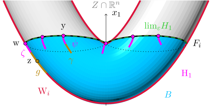
Figure 10: Illustration of proof of Lemma 4.4 with $\bm{\varphi}_{1}=\pi_{1}$ and $V$ is isomorphic to $\bm{V}(x_{1}^{2}+x_{2}^{2}-1)\times{\color[rgb]{0,0,0}\bm{V}(x_{1}-x_{2}^{2})}$. Elements of $H_{1}$ can be seen as curves of infinitesimal lengths, starting from a point of $\operatorname{lim_{\varepsilon}}H_{1}$, and lying in $B$. Here, $\operatorname{lim_{\varepsilon}}H_{1}$ is the set of points that share the same first coordinate than ${\bm{y}}$. Hence, the above proof consisted in choosing a $\zeta$ in $H_{1}$, that lives “inside” $W_{i}\cup\operatorname{sing}(V)$ (actually in $\operatorname{ext}(W_{i}\cup\operatorname{sing}(V),\mathbf{R}\langle\varepsilon\rangle)$).

We can now prove Proposition 4.2. This proof is illustrated by Figure 10.

Proof of Proposition 4.2.

Let $B$ be a semi-algebraically connected component of $C_{\mid\bm{\varphi}_{1}<u}$. Since $\bm{\varphi}_{1}$ is a proper map bounded from below on $V\cap\mathbf{R}^{n}$ by assumption $\mathsf{P}$, $C_{\mid\bm{\varphi}_{1}<u}$, and then $B$, are bounded. Then applying Proposition 3.6 shows that:

$$\emptyset\;\subsetneq\;B\cap K(\bm{\varphi}_{1},V)\;\subset\;B\cap F_{i}\;\subset\;B\cap(F_{i}\cup W_{i}).$$

The first item is then proved. Let ${\bm{y}}\in\overline{B}\cap(F_{i}\cup W_{i})$. To prove the second item, one only needs to consider the case where ${\bm{y}}\in\overline{B}\cap(W_{i}-F_{i})$ according to Lemma 4.4. Moreover one can assume that ${\bm{y}}\notin B$ and then $\bm{\varphi}_{1}({\bm{y}})=u$, otherwise, taking ${\bm{z}}={\bm{y}}$, would end the proof.

Let $D$ be the semi-algebraically connected component of $(W_{i})_{\mid\bm{\varphi}_{1}\leq u}$ containing ${\bm{y}}$. We consider two disjoint cases.

1. If $D\not\subset\overline{B}$, there exists ${\bm{y}}^{\prime}\in D$ such that ${\bm{y}}^{\prime}\notin\overline{B}$. Then let $\gamma\colon[0,1]\rightarrow D$ such that $\gamma(0)={\bm{y}}$ and $\gamma(1)={\bm{y}}^{\prime}$. Hence, if

   $$t_{1}=\max\{t\in[0,1)\mid\gamma(t)\in\overline{B}\},$$

   then $\gamma(t_{1})\in K(\bm{\varphi}_{1},V)$ by the contrapositive of statement $c)$ of Lemma 3.3. Since $K(\bm{\varphi}_{1},V)\subset F_{i}$, we can apply Lemma 4.4 to $\gamma(t_{1})$ and find ${\bm{z}}\in B\cap(F_{i}\cup W_{i})$ that is connected to $\gamma(t_{1})$ and then to ${\bm{y}}$ by a semi-algebraic path in $\overline{B}\cap(F_{i}\cup W_{i})$.

2. If $\mathit{D\subset\overline{B}}$, we claim that there exists some ${\bm{z}}\in D\cap F_{i}$. Indeed since $D$ is a semi-algebraically connected component of $(W_{i})_{\mid\bm{\varphi}_{1}\leq u}$ and $\bm{\varphi}_{1}$ is a proper map, $D$ is bounded. Then by Proposition 3.6 there exists ${\bm{y}}^{\prime}\in D\cap K(\bm{\varphi}_{1},W_{i})$. If ${\bm{y}}^{\prime}\in\operatorname{sing}(W_{i})$ then ${\bm{y}}^{\prime}\in\operatorname{sing}(V)$ by assumption $\mathsf{B}_{1}$ and taking ${\bm{z}}={\bm{y}}^{\prime}\in F_{i}$ one concludes as in the first item.

   Else ${\bm{y}}^{\prime}$ is in $W(\bm{\varphi}_{1},W_{i})$, and we let $E$ be the semi-algebraically connected component of $W(\bm{\varphi}_{1},W_{i})$ containing ${\bm{y}}^{\prime}$. Since $\bm{\varphi}_{1}(W(\bm{\varphi}_{1},W_{i}))$ is finite by Sard’s lemma, $\bm{\varphi}_{1}(E)=\{\bm{\varphi}_{1}({\bm{y}}^{\prime})\}$, so that $E\subset(W_{i})_{\mid\bm{\varphi}_{1}\leq u}$. Hence, since $E$ is semi-algebraically connected, $E\subset D$. By assumption $\mathsf{C}_{2}$, there exists ${\bm{z}}\in E\cap{\color[rgb]{0,0,0}S_{i}}$, so that ${\bm{z}}\in D\cap{\color[rgb]{0,0,0}S_{i}}\subset D\cap F_{i}$ and we are done.

   Then we can connect ${\bm{y}}$ to ${\bm{z}}$ inside $D\subset\overline{B}\cap W_{i}$ and since ${\bm{z}}$ is in $D\cap F_{i}$, which is contained in $\overline{B}\cap F_{i}$, we can connect similarly ${\bm{z}}$ to some ${\bm{z}}^{\prime}\in B\cap(F_{i}\cup W_{i})$ inside $\overline{B}\cap F_{i}$ by Lemma 4.4. Putting things together, ${\bm{y}}$ is connected to some ${\bm{z}}^{\prime}\in B\cap(F_{i}\cup W_{i})$ by a semi-algebraic path in $\overline{B}\cap F_{i}$.
   

∎

Corollary 4.5.

Let $u\in\mathbf{R}$ such that for all $u^{\prime}<u$, $\mathrm{RM}(u^{\prime})$ holds. Let $C$ be a semi-algebraically connected component of $V_{\mid\bm{\varphi}_{1}\leq u}$ such that $C_{\mid\bm{\varphi}_{1}<u}$ is non-empty. If $B$ is a semi-algebraically connected component of $C_{\mid\bm{\varphi}_{1}<u}$, then $\overline{B}\cap\mathscr{R}$ is non-empty and semi-algebraically connected.

Proof.

Let ${\bm{y}}$ and ${\bm{y}}^{\prime}$ be in $\overline{B}\cap\mathscr{R}$. According to Proposition 4.2, they can respectively be connected to some ${\bm{z}}$ and ${\bm{z}}^{\prime}$ in $B\cap\mathscr{R}$, by a semi-algebraic path in $\overline{B}\cap\mathscr{R}$. As $B$ is semi-algebraically connected, there exists a semi-algebraic path $\gamma\colon[0,1]\rightarrow B$ connecting ${\bm{z}}$ to ${\bm{z}}^{\prime}$. Let

$$u^{\prime}=\max\big{\{}\bm{\varphi}_{1}(\gamma(t))\mid t\in[0,1]\big{\}},$$

so that $\gamma([0,1])\subset V_{\mid\bm{\varphi}_{1}\leq u^{\prime}}$. Such a $u^{\prime}$ exists by continuity of $\gamma$, and satisfies $u^{\prime}<u$, as $[0,1]$ is closed and bounded.

Let $B^{\prime}$ be the semi-algebraically connected component of $B_{\mid\bm{\varphi}_{1}\leq u^{\prime}}$ that contains $\gamma([0,1])$. Since $B^{\prime}$ is also a semi-algebraically connected component of $V_{\mid\bm{\varphi}_{1}\leq u^{\prime}}$, property $\mathrm{RM}(u^{\prime})$ states that $B^{\prime}\cap\mathscr{R}$ is non-empty and semi-algebraically connected. Then, as ${\bm{z}}$ and ${\bm{z}}^{\prime}$ are in $B^{\prime}\cap\mathscr{R}$, they can be connected by a semi-algebraic path in $B^{\prime}\cap\mathscr{R}$, and then, in $B\cap\mathscr{R}$. Thus ${\bm{y}}$ and ${\bm{y}}^{\prime}$ are connected by a semi-algebraic path in $\overline{B}\cap\mathscr{R}$ and we are done. ∎

4.2 Recursive proof of the truncated roadmap property

In order to prove that $\mathrm{RM}(u)$ holds for all $u\in\mathbf{R}$, one can consider two disjoint cases: whether $u$ is a real singular value of $\bm{\varphi}_{1}$, that is $u\in\bm{\varphi}_{1}(K_{i})$, or not. The following lemma allows us to proceed by induction.

Lemma 4.6.

The set $\bm{\varphi}_{1}(K_{i})$ is non-empty and finite.

Proof.

By the algebraic version of Sard’s theorem [24, Proposition B.2], the set of critical values of $\bm{\varphi}_{1}$ on $V$ is an algebraic set of $\mathbf{C}$ of dimension 0. Then, it is either empty or non-empty but finite. Hence, $\bm{\varphi}_{1}(K_{i})$ is either empty or non-empty but finite, as ${\color[rgb]{0,0,0}S_{i}}$ and $\operatorname{sing}(V)$ are, by assumption. Moreover since $\bm{\varphi}_{1}$ is a proper map bounded from below on $V\cap\mathbf{R}^{n}$ by assumption $(\mathsf{P})$, for any $u\in\mathbf{R}$, $Z_{\mid\bm{\varphi}<u}$ is bounded. Then, since $V$ is not empty, by Proposition 3.6 the sets $K(\bm{\varphi}_{1},V)$ and then $\bm{\varphi}_{1}(K_{i})$ are not empty. ∎

We denote by $v_{1}<\dotsc<v_{\ell}$ the points of $\bm{\varphi}_{1}(K_{i}\cap\mathbf{R}^{n})$ and, in addition, let $v_{\ell+1}=+\infty$. We proceed by proving the two following steps.

Step 1:

Let $u\in\mathbf{R}$, if $\mathrm{RM}(u^{\prime})$ holds for all $u^{\prime}<u$, then $\mathrm{RM}(u)$ holds.

Step 2:

Let $j\in\{1,\dotsc,\ell\}$, if $\mathrm{RM}(v_{j})$ holds, then for all $u\in(v_{j},v_{j+1})$, $\mathrm{RM}(u)$ holds.

Remark that, by Lemma 3.5, $v_{1}=\min_{V\cap\mathbf{R}^{n}}\bm{\varphi}_{1}$, since $V\cap\mathbf{R}^{n}$ is closed. Then for $u^{\prime}<v_{1}$, $V_{\mid\bm{\varphi}\leq u^{\prime}}=\emptyset$ and $\mathrm{RM}(u^{\prime})$ trivially holds. Hence, proving these two steps is enough to prove $\mathrm{RM}(u)$ for all $u$ in $\mathbf{R}$, by an immediate induction.

Proposition 4.7 (Step 1).

Let $u\in\mathbf{R}$. Assume that for all $u^{\prime}<u$, $\mathrm{RM}(u^{\prime})$ holds. Then $\mathrm{RM}(u)$ holds.

The proof of this proposition is illustrated by Figure 11.

Proof.

Let $u\in\mathbf{R}$ be such that for all $u^{\prime}<u$, $\mathrm{RM}(u^{\prime})$ holds and let $C$ be a semi-algebraically connected component of $V_{\mid\bm{\varphi}_{1}\leq u}$. We have to prove that $C\cap\mathscr{R}$ is non-empty and semi-algebraically connected.

If $C_{\mid\bm{\varphi}_{1}<u}$ is empty, then, by Lemma 3.5, $C\subset K(\bm{\varphi}_{1},V)$. But the points of $K(\bm{\varphi}_{1},V)$ are either in $W_{i}$ or in $\operatorname{sing}(V)\subset F_{i}$. Hence $K(\bm{\varphi}_{1},V)\subset\mathscr{R}$ and $C\cap\mathscr{R}=C$, which is non-empty and semi-algebraically connected by definition.

From now on, $C_{\mid\bm{\varphi}_{1}<u}$ is supposed to be non-empty and let $B_{1},\dotsc,B_{r}$ be its semi-algebraically connected components. According to Corollary 4.5, for all $1\leq j\leq r$, $\overline{B_{j}}\cap\mathscr{R}$ is non-empty and semi-algebraically connected. Then, as $\overline{B_{j}}\subset C$,

$$\overline{B_{j}}\cap\mathscr{R}\subset C\cap\mathscr{R}$$

for every $1\leq j\leq r$, and $C\cap\mathscr{R}$ is non-empty.

Let us now prove that $C\cap\mathscr{R}$ is semi-algebraically connected. Let ${\bm{y}}$ and ${\bm{y}}^{\prime}$ in $C\cap\mathscr{R}$. As $C$ is semi-algebraically connected, there exists a semi-algebraically continuous map $\gamma\colon[0,1]\rightarrow C$ such that $\gamma(0)={\bm{y}}$ and $\gamma(1)={\bm{y}}^{\prime}$. Now let

$$G=\gamma^{-1}(C_{\mid\bm{\varphi}_{1}=u}\cap K(\bm{\varphi}_{1},V))\quad\text{and}\quad H=[0,1]-G.$$

We denote by $G_{1},\dotsc,G_{N}$ the connected components of $G$ and $H_{1},\dotsc,H_{M}$ those of $H$. The sets $H_{j}$ for $1\leq j\leq M$ are open intervals of $[0,1]$, and we note $\ell_{j}=\inf(H_{j})$ and $r_{j}=\sup(H_{j})$. Since $\gamma(G)$ already lies in $C\cap\mathscr{R}$, let us establish that for every $1\leq j\leq M$, $\gamma(\ell_{j})$ and $\gamma(r_{j})$ can be connected by another semi-algebraic path $\tau_{j}$ in $C\cap\mathscr{R}$.

Let $1\leq j\leq M$, then $\gamma(H_{j})\cap(C_{\mid\bm{\varphi}_{1}=u}\cap K(\bm{\varphi}_{1},V))=\emptyset$ by definition. Moreover, $\gamma(H_{j})\subset C$ so that

$$\gamma(H_{j})\cap(V_{\mid\bm{\varphi}_{1}=u}\cap K(\bm{\varphi}_{1},V))=\emptyset.$$

Hence, since $H_{j}$ is connected, there exists (by Proposition 3.1) a unique semi-algebraically connected component $B$ of $V_{\mid\bm{\varphi}_{1}<u}$ such that $\gamma(H_{j})\subset\overline{B}$. But $\gamma(H_{j})\subset C$, so that $\overline{B}$ and thus $B$ are actually contained in $C$. Therefore, $B$ is actually a semi-algebraically connected component of $C_{\mid\bm{\varphi}_{1}<u}$ and there exists $1\leq k\leq r$ such that $B=B_{k}$. At this step $\gamma(H_{j})\subset\overline{B_{k}}$, so that

$$\gamma([\ell_{j},r_{j}])=\gamma(\overline{H_{j}})\;\subset\;\overline{\gamma(H_{j})}\;\subset\;\overline{B_{k}},$$

and both $\gamma(\ell_{j})$ and $\gamma(r_{j})$ are in $\overline{B_{k}}$. Remark that both $\ell_{j}$ and $r_{j}$ are in $G$, so that both $\gamma(\ell_{j})$ and $\gamma(r_{j})$ are in $K(\bm{\varphi}_{1},V)\subset F_{i}\subset\mathscr{R}$. Thus, both $\gamma(\ell_{j})$ and $\gamma(r_{j})$ are in $\overline{B_{k}}\cap\mathscr{R}$. According to Corollary 4.5, they can be connected by a semi-algebraic path $\tau_{j}\colon[0,1]\to\overline{B_{k}}\cap\mathscr{R}\subset C\cap\mathscr{R}$.

In conclusion, we have proved that for $1\leq j\leq M$, $\gamma(\ell_{j})$ and $\gamma(r_{j})$ can be connected by a semi-algebraic path $\tau_{j}$ in $C\cap\mathscr{R}$. Therefore the semi-algebraic sub-paths $\gamma_{\mid H_{j}}$ can be replaced by the $\tau_{j}$’s, which lie in $C\cap\mathscr{R}$. Moreover, for all $1\leq j\leq N$

$$\gamma(G_{j})\subset C\cap\mathscr{R}.$$

Since the $H_{j}$’s and $G_{j}$’s form a partition of $[0,1]$, by putting together alternatively the $\tau_{j}$’s and the $\gamma_{\mid G_{j}}$’s, one obtains a semi-algebraic path in $C\cap\mathscr{R}$ connecting ${\bm{y}}=\gamma(0)$ to ${\bm{y}}^{\prime}=\gamma(1)$. And we are done. ∎

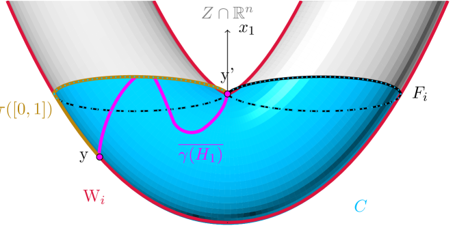
Figure 11: Illustration of proof of Proposition 4.7 with $\bm{\varphi}_{1}=\pi_{1}$ and $V$ is isomorphic to $\bm{V}(x_{1}^{2}+x_{2}^{2}-1)\times{\color[rgb]{0,0,0}\bm{V}(x_{1}-x_{2}^{2})}$. Here, only ${\bm{y}}^{\prime}$ belongs to $C_{\mid\pi_{1}=u}\cap K(\pi_{1},V)$. Then we replace the path $\gamma=\gamma_{\mid H_{1}}$ by a path $\tau_{1}$ that lies in the intersection of the roadmap and the semi-algebraically connected component $C$.

Proposition 4.8 (Step 2).

Let $j\in\{1,\dotsc,\ell\}$, if $\mathrm{RM}(v_{j})$ holds, then for all $u\in(v_{j},v_{j+1})$, $\mathrm{RM}(u)$ holds.

The proof of this proposition is illustrated by Figure 12.

Proof.

Let $j\in\{0,\dotsc,\ell\}$ and $u\in(v_{j},v_{j+1})$. Let $C$ be a semi-algebraically connected component of $V_{\mid\bm{\varphi}_{1}\leq u}$; we have to prove that $C\cap\mathscr{R}$ is non-empty and semi-algebraically connected.

Let us first prove that $C_{\mid\bm{\varphi}_{1}\leq v_{j}}\cap\mathscr{R}$ is non-empty and semi-algebraically connected. By assumption $(\mathsf{A})$, $V$ is an equidimensional algebraic set of positive dimension, and by assumption $(\mathsf{P})$, the restriction of $\bm{\varphi}_{1}$ to $V\cap\mathbf{R}^{n}$ is a proper map bounded below. Moreover, as $\bm{\varphi}_{1}\left(K(\bm{\varphi}_{1},V)\cap\mathbf{R}^{n}\right)\subset\{v_{1},\dotsc,v_{\ell}\}$, then

$$V_{\mid\bm{\varphi}_{1}\in(v_{j},u]}\cap K(\bm{\varphi}_{1},V)=\emptyset.$$

Then using Corollary 3.10, one deduces that $C_{\mid\bm{\varphi}_{1}\leq v_{j}}$ is a semi-algebraically connected component of $V_{\mid\bm{\varphi}_{1}\leq v_{j}}$. Hence, by property $\mathrm{RM}(v_{j})$, the set $C_{\mid\bm{\varphi}_{1}\leq v_{j}}\cap\mathscr{R}$ is non-empty and semi-algebraically connected. In particular, $C\cap\mathscr{R}$ is non-empty.

Let us now prove that $C\cap\mathscr{R}$ is semi-algebraically connected. Let ${\bm{y}}$ be in $C\cap\mathscr{R}$. According to the previous paragraph, one just need to be able to connect ${\bm{y}}$ to a point ${\bm{z}}$ of $C_{\mid\bm{\varphi}_{1}\leq v_{j}}\cap\mathscr{R}$ by a semi-algebraic path in $C\cap\mathscr{R}$ and then apply $\mathrm{RM}(v_{j})$. First, if ${\bm{y}}\in C_{\mid\bm{\varphi}_{1}\leq v_{j}}\cap\mathscr{R}$, there is nothing to do. Suppose now that ${\bm{y}}\in C_{\mid\bm{\varphi}_{1}\in(v_{j},u]}\cap\mathscr{R}$. We claim that actually

$${\bm{y}}\in C\cap W_{i}.$$

Indeed, if ${\bm{y}}\in C\cap F_{i}$, then $\bm{\varphi}_{i-1}({\bm{y}})\in\bm{\varphi}_{i-1}(K_{i})$ and $\bm{\varphi}_{1}({\bm{y}})$ would be one of the $v_{1},\dotsc,v_{\ell}$.

Let $D$ be the semi-algebraically connected component of $(C\cap W_{i})_{\mid\bm{\varphi}_{1}\leq u}$ containing ${\bm{y}}$. Remark that $D$ is a semi-algebraically connected component of $(W_{i})_{\mid\bm{\varphi}_{1}\leq u}$, as it contains ${\bm{y}}$ and is contained in $C$. Since $\bm{\varphi}_{1}(W(\bm{\varphi}_{1},W_{i}))$ is finite by Sard’s lemma, we get that $\bm{\varphi}_{1}(W(\bm{\varphi}_{1},W_{i}))\subset\bm{\varphi}_{1}({\color[rgb]{0,0,0}S_{i}})$, by assumption $(\mathsf{C}_{2})$, so that

$$(v_{j},u)\cap\bm{\varphi}_{1}(W(\bm{\varphi}_{1},W_{i}))=\emptyset.$$

Since $W_{i}$ is equidimensional and smooth outside $\operatorname{sing}(V)$, then by Corollary 3.10, $D_{\mid\bm{\varphi}_{1}\leq v_{j}}$ is a semi-algebraically connected component of $(W_{i})_{\mid\bm{\varphi}_{1}\leq v_{j}}$. Therefore, let ${\bm{z}}\in D_{\mid\bm{\varphi}_{1}\leq v_{j}}$. Since $D$ is semi-algebraically connected, there exists a semi-algebraic path, connecting ${\bm{y}}\in D\subset C\cap\mathscr{R}$ to

$${\bm{z}}\in D_{\mid\bm{\varphi}_{1}\leq v_{j}}\subset C_{\mid\bm{\varphi}_{1}\leq v_{j}}\cap\mathscr{R}$$

in $D\subset C\cap\mathscr{R}$. We are done. ∎

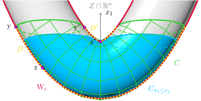
Figure 12: Illustration of proof of Proposition 4.8 with $\bm{\varphi}_{1}=\pi_{1}$ and $V$ is isomorphic to $\bm{V}(x_{1}^{2}+x_{2}^{2}-1)\times{\color[rgb]{0,0,0}\bm{V}(x_{1}-x_{2}^{2})}$. We connect the points ${\bm{y}}$ and ${\bm{y}}^{\prime}$ in $C\cap W_{i}$ to respectively ${\bm{z}}$ and ${\bm{z}}^{\prime}$ in $C_{\mid\pi_{1}\leq v_{j}}$. Then we are reduced to the case of Step 1.

5 Conclusions and perspectives

We illustrate below two ways of using Theorem 1.1 in order to generalize the algorithms of [24] to the case of unbounded smooth real algebraic sets.

Let $V\subset\mathbf{C}^{n}$ be an equidimensional algebraic set of dimension $d$ given as the solutions of some polynomials $f_{1},\ldots,f_{p}$ in $\mathbf{Q}[x_{1},\ldots,x_{n}]$. Assume that $\operatorname{sing}(V)$ is finite. Take

$$\varphi_{1}=\sum_{k=1}^{n}(x_{k}-\bm{a}_{k})^{2}\quad\text{and for\> $2\leq j\leq n$}\quad\varphi_{j}=\sum_{k=1}^{n}\bm{b}_{j,k}x_{k},\qquad$$

where $\bm{a}=(\bm{a}_{1},\dotsc,\bm{a}_{n})\in\mathbf{Q}^{n}$ and, for $2\leq j\leq n$, $\bm{b}_{j}=(\bm{b}_{j,1},\dotsc,\bm{b}_{j,n})\in\mathbf{Q}^{n}$. Then, assumption $(\mathsf{P})$ holds. Also, according to [2, 3], for a generic choice of $\bm{a}$ and $\bm{b}$, the dimension properties of assumption $(\mathsf{B})$ do hold.

For some chosen $2\leq i\leq d$, let $W_{i}$ and $F_{i}$ be respectively the polar variety and set of fibers as defined in the introduction. One can compute a set $S\subset W(\varphi_{1},W_{i})\subset V$ by using any algorithm such as [4, Chap. 13] or [22], returning sample points in all connected components of real algebraic sets.

Hence, one can apply Theorem 1.1 to $V$, $\bm{\varphi}$ and $i$. We deduce that $W_{i}\cup F_{i}$ has a non-empty and connected intersection with all connected components of $V\cap\mathbf{R}^{n}$, but it is in general an object of dimension greater than $1$, so more work is needed.

Our first option is to recursively perform similar operations, using this time polynomials defining respectively $W_{i}$ and $F_{i}$, eventually building a roadmap for $V$ itself (this is justified by [23, Prop. 2]). This requires that both $W_{i}$ and $F_{i}$ are equidimensional with finitely many singular points.

The cost of the whole procedure will depend on the degrees of $W_{i}$ and $F_{i}$. Denote by $D$ the degrees of the $f_{i}$’s and by $\delta$ (resp. $\sigma$) the degree of $V$ (resp. $S$); using [4, Chap. 13] gives $\sigma\in D^{O(n)}$. Assuming that $d=n-p$ and that the ideal generated by $f_{1},\ldots,f_{p}$ is radical, one can apply Heintz’s version of the Bézout theorem [18] as in [22] to deduce that $\delta\leq D^{p}$ and that the degree of $W_{i}$ is bounded by $\delta(nD)^{n-p}\in(nD)^{O(n)}$. Similarly, one can expect that the degree $\delta^{\prime}$ of $W(\varphi_{1},W_{i})$ lies in $(nD)^{O(n)}$ by applying similar arguments to those used in [24]. Since the degree of $F_{i}$ is bounded by the product of $\delta$ and $\delta^{\prime}+\sigma$, we deduce that its degree also lies in $(nD)^{O(n)}$.

Hence, as explained in [23], the overall complexity of such recursive algorithms is $(nD)^{O(nr)}$, where $r$ is the depth of the recursion, provided that the involved geometric sets do satisfy the properties needed by Theorem 1.1 and can be represented and computed with algebraic data within complexities which are polynomial in their degrees.

To understand the possible depth of recursion one could expect, one also needs to have a look at the dimensions of $W_{i}$ and $F_{i}$. Observe that $W_{i}$ is expected to have dimension $i-1$. Similarly, $F_{i}$ is expected to have dimension $d-(i-1)$. Taking $i\simeq\lfloor\frac{\dim(V)}{2}\rfloor$ will decrease the dimensions of $W_{i}$ and $F_{i}$ to $\simeq\lfloor\frac{\dim(V)}{2}\rfloor$ if they are not empty (this will require coordinates). Hence the depth $r$ of this new recursive roadmap algorithm will be bounded by $\log_{2}(n)$.

A second approach to design our new algorithm takes $i=2$. Then, $W_{2}$ is expected to have dimension $1$ (or be empty), so no further computation is needed. On the other hand, $F_{2}$ still has dimension $d-1$, but a key observation is that $F_{2}$ is now bounded. Then, one can directly apply a slight variant of the algorithm in [24] taking $F_{2}$ as input: that algorithm already keeps the depth of recursion bounded by $\log_{2}(n)$, but we should now handle the fact that we work in the hypersurface $\varphi_{1}^{-1}(\varphi_{1}(K_{1}))$. Again, all of this is under the assumption that one can make $F_{2}$ satisfy the assumptions of Theorem 1.1.

We will investigate that approach in a forthcoming paper.

Thus, the next steps to obtain nearly optimal algorithms for computing roadmaps of smooth real algebraic sets, without compactness assumptions, are:

• to study how the constructions of generalized Lagrange systems introduced in [24] for encoding polar varieties associated to linear projections can be reused in our context;

• to prove that assumption $(\mathsf{B})$ holds for some generic choice of $\bm{a}$ and $\bm{b}$ for our polar varieties, which by contrast to those used in [24] are no more associated to linear projections;

• to prove that the variant of the algorithm designed in [24] discussed above still has a complexity similar to the one obtained in [24].

The example below illustrates how this whole machinery might work and how Theorem 1.1 can already be used.

Example 1.

Let $V=\bm{V}(g)\subset\mathbb{C}^{3}$ be the hypersurface defined by the vanishing set of the polynomial $g=x_{1}^{3}+x_{2}^{3}+x_{3}^{3}-x_{1}-x_{2}-x_{3}-1\in\mathbb{Q}[x_{1},x_{2},x_{3}]$. As a hypersurface, $V$ is 2-equidimensional and since $\operatorname{sing}(V)=\emptyset$, $V$ satisfies $(\mathsf{A})$.

Let ${\color[rgb]{0,0,0}\bm{\varphi}=((x_{1}-1)^{2}+x_{2}^{2}+x_{3}^{2},\>x_{1},\>x_{2})}\subset\mathbb{Q}[x_{1},x_{2},x_{3}]$. As the restriction of $\bm{\varphi}_{1}$ to $\mathbb{R}^{n}$ is the square of the Euclidean distance to $(1,0,0)$, $(\mathsf{P})$ is satisfied. Since $2\leq i\leq d$, we must take $i=2$. Then we see that one can write

$$W_{2}=\bm{V}(f,{\color[rgb]{0,0,0}(3x_{1}x_{3}+1)(x_{1}-x_{3})+3x_{3}^{2}-1}).$$

One checks that $W_{2}$ is 1-equidimensional and has no singular point as well, so that $(\bm{\varphi},2)$ satisfies $(\mathsf{B}_{1})$. Let $K_{2}=W^{\circ}(\bm{\varphi}_{1},W_{2})$, which is a finite set of cardinality $45$ (of which $5$ are real). Besides, for any $\alpha\in\mathbb{C}$,

$$V\cap\bm{\varphi}_{1}^{-1}(\alpha)={\color[rgb]{0,0,0}\bm{V}(f,(x_{1}-1)^{2}+x_{2}^{2}+x_{3}^{2}-\alpha)}$$

is either empty or an equidimensional algebraic set of dimension 1. Therefore, $(\bm{\varphi},2)$ satisfies $(\mathsf{B})$. Finally, since $W^{\circ}(\bm{\varphi}_{1},W_{2})\cap\mathbb{R}^{3}$ is a finite set, assumption $(\mathsf{C})$ holds vacuously. Recall that, by definition, $F_{2}={\bm{\varphi}_{1}}^{-1}(\bm{\varphi}_{1}(K_{2}))\cap V$. In conclusion, by Theorem 1.1, $W_{2}\cup F_{2}$ is a $1$-roadmap of $(V,\emptyset)$. Figure 13 illustrates this example.

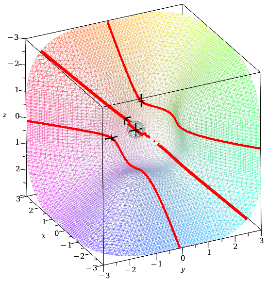
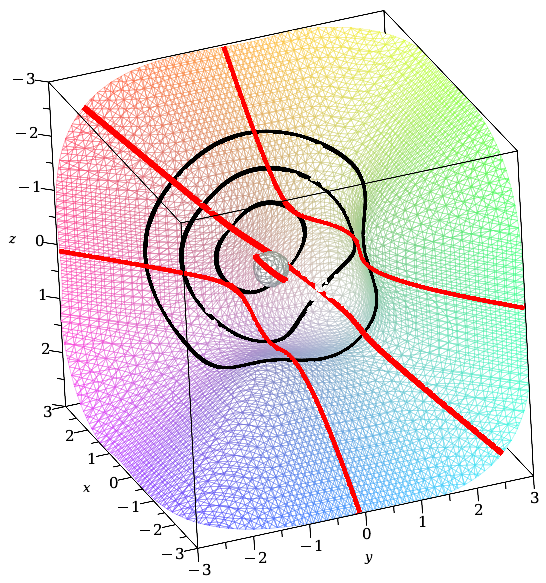
Figure 13: An illustration of Example 1. The real trace $V\cap\mathbb{R}^{3}$ is plotted twice as a grid. On the left, $W_{2}\cap\mathbb{R}^{3}$ is represented as red lines, and the crosses represent all the real points of $K_{2}$. Then, on the right, we replaced the points of $K_{2}$ by the fibers of $F_{2}\cap\mathbb{R}^{3}$ (black lines), to repair the connectivity failures of $W_{2}\cap\mathbb{R}^{3}$. In particular, $F_{2}\cap\mathbb{R}^{3}$ connects the semi-algebraically connected components of $W_{2}\cap\mathbb{R}^{3}$ that lie in the same semi-algebraically connected component of $V\cap\mathbb{R}^{3}$.

We expect that algorithmic progress on the computation of roadmaps for real algebraic and semi-algebraic sets will lead to implementations that will automate the analysis of kinematic singularities for e.g. serial and parallel manipulators. In particular, there are many families of robots where these algorithms could be used if they scale enough. This is the case for e.g. 6R manipulators (see e.g. the results on the number of aspects in [28] which need to be extended) in the context of serial manipulators, for the study of self-motion spaces of parallel platforms such as Gough-Stewart ones (the case of such manipulators with $6$ lengths still remains open, see e.g. [21]) and for the identification of cuspidality manipulators (see [14] for a general approach, relying on roadmap algorithms). For some of these applications, one needs to compute the number of connected components of semi-algebraic sets defined as the complement of a real hypersurface defined by $f=0$ where $f$ is a multivariate polynomial. Note that this can be done by computing a roadmap for the (non-bounded) real algebraic set defined by $tf-1=0$ where $t$ is a new variable. This illustrates the potential interest of the algorithms that would be derived from the connectivity theorem of this paper.

References

- [1] B. Bank, M. Giusti, J. Heintz, and L. M. Pardo. Generalized polar varieties and an efficient real elimination. Kybernetika, 40(5):519–550, 2004.
- [2] B. Bank, M. Giusti, J. Heintz, and L. M. Pardo. Generalized polar varieties: Geometry and algorithms. Journal of complexity, 21(4):377–412, 2005.
- [3] B. Bank, M. Giusti, J. Heintz, M. Safey El Din, and E. Schost. On the geometry of polar varieties. Applicable Algebra in Engineering, Communication and Computing, 21(1):33–83, 2010.
- [4] S. Basu, R. Pollack, and M.-F. Roy. Algorithms in Real Algebraic Geometry. 10. Springer, Berlin, Heidelberg, 3 edition, 2016.
- [5] S. Basu and M.-F. Roy. Divide and conquer roadmap for algebraic sets. Discrete & Computational Geometry, 52(2):278–343, 2014.
- [6] S. Basu, M.-F. Roy, M. Safey El Din, and É. Schost. A baby step–giant step roadmap algorithm for general algebraic sets. Foundations of Computational Mathematics, 14(6):1117–1172, 2014.
- [7] J. Bochnak, M. Coste, and M.-F. Roy. Real algebraic geometry, volume 36. Springer Science & Business Media, 2013.
- [8] J. Canny. The complexity of robot motion planning. MIT press, 1988.
- [9] J. Canny. Constructing roadmaps of semi-algebraic sets i: Completeness. Artificial Intelligence, 37(1-3):203–222, 1988.
- [10] J. Canny. Computing roadmaps of general semi-algebraic sets. The Computer Journal, 36(5):504–514, 1993.
- [11] J. F. Canny. Computing roadmaps of general semi-algebraic sets. In International Symposium on Applied Algebra, Algebraic Algorithms, and Error-Correcting Codes, pages 94–107. Springer, 1991.
- [12] J. Capco, M. Safey El Din, and J. Schicho. Robots, computer algebra and eight connected components. In Proceedings of the 45th International Symposium on Symbolic and Algebraic Computation, pages 62–69, 2020.
- [13] J. Capco, M. Safey El Din, and J. Schicho. Positive dimensional parametric polynomial systems, connectivity queries and applications in robotics. Journal of Symbolic Computation, 115:320–345, 2023.
- [14] D. Chablat, R. Prébet, M. Safey El Din, D. H. Salunkhe, and P. Wenger. Deciding cuspidality of manipulators through computer algebra and algorithms in real algebraic geometry. In Proceedings of the 2022 International Symposium on Symbolic and Algebraic Computation, ISSAC ’22, page 439–448, New York, NY, USA, 2022. Association for Computing Machinery.
- [15] C. Chen, W. Wu, and Y. Feng. A numerical roadmap algorithm for smooth bounded real algebraic surface. In Polynomial Computer Algebra, pages 43–48, 2019.
- [16] M. Coste and M. Shiota. Nash triviality in families of nash manifolds. Inventiones mathematicae, 108(1):349–368, 1992.
- [17] D. Grigoryev and N. Vorobjov. Counting connected components of a semialgebraic set in subexponential time. Computational Complexity, 2:133–186, 06 1992.
- [18] J. Heintz. Definability and fast quantifier elimination in algebraically closed fields. Theoretical Computer Science, 24(3):239–277, 1983.
- [19] R. Iraji and H. Chitsaz. Nuroa: A numerical roadmap algorithm. In 53rd IEEE Conference on Decision and Control, pages 5359–5366. IEEE, 2014.
- [20] M. Mezzarobba and M. Safey El Din. Computing roadmaps in smooth real algebraic sets. In Transgressive Computing 2006, pages 327–338, 2006.
- [21] G. Nawratil and J. Schicho. Self-motions of pentapods with linear platform. Robotica, 35(4):832–860, 2017.
- [22] M. Safey El Din and E. Schost. Polar varieties and computation of one point in each connected component of a smooth real algebraic set. In Proceedings of the 2003 International Symposium on Symbolic and Algebraic Computation, ISSAC ’03, page 224–231, New York, NY, USA, 2003. Association for Computing Machinery.
- [23] M. Safey El Din and É. Schost. A baby steps/giant steps probabilistic algorithm for computing roadmaps in smooth bounded real hypersurface. Discrete & Computational Geometry, 45(1):181–220, 2011.
- [24] M. Safey El Din and É. Schost. A nearly optimal algorithm for deciding connectivity queries in smooth and bounded real algebraic sets. Journal of the ACM (JACM), 63(6):1–37, 2017.
- [25] J. T. Schwartz and M. Sharir. On the “piano movers” problem. ii. general techniques for computing topological properties of real algebraic manifolds. Advances in applied Mathematics, 4(3):298–351, 1983.
- [26] I. R. Shafarevich. Basic Algebraic Geometry, volume 1. Springer, 1994.
- [27] N. Vorobjov and D. Y. Grigoriev. Determination of the number of connected components of a semi-algebraic set in subexponential time. Dokl. Akad. Nauk SSSR, 314(5), 1990.
- [28] P. Wenger. Cuspidal and noncuspidal robot manipulators. Robotica, 25(6):677–689, 2007.