Graph Reinforcement Learning for Radio Resource Allocation

Abstract

Deep reinforcement learning (DRL) for resource allocation has been investigated extensively owing to its ability of handling model-free and end-to-end problems. Yet the high training complexity of DRL hinders its practical use in dynamic wireless systems. To reduce the training cost, we resort to graph reinforcement learning for exploiting two kinds of relational priors inherent in many problems in wireless communications: topology information and permutation properties. To design graph reinforcement learning framework systematically for harnessing the two priors, we first conceive a method to transform state matrix into state graph, and then propose a general method for graph neural networks to satisfy desirable permutation properties. To demonstrate how to apply the proposed methods, we take deep deterministic policy gradient (DDPG) as an example for optimizing two representative resource allocation problems. One is predictive power allocation that minimizes the energy consumed for ensuring the quality-of-service of each user that requests video streaming. The other is link scheduling that maximizes the sum-rate for device-to-device communications. Simulation results show that the graph DDPG algorithm converges much faster and needs much lower space complexity than existing DDPG algorithms to achieve the same learning performance.

I Introduction

Deep reinforcement learning (DRL) has been introduced to optimize a variety of resource allocation problems, thanks to its ability of learning wireless policies from the optimization problems without closed-form objectives and constraints, making decision in an end-to-end manner, and online training [1, 2, 3, 4, 5, 6, 7, 8].

When learning a resource allocation policy to be operated in non-stationary wireless channels, a DRL algorithm needs to be online trained consistently for adapting to the dynamic environments. In particular, the agent of DRL interacts with the environment to gather a sample (i.e., an experience in reinforcement learning parlance) in each time step and updates deep neural networks (DNNs) with a batch of experiences every several time steps. Before a DRL algorithm converges, the decision made by the algorithm is with unacceptable performance.

Existing DRL algorithms suffer from high training complexity, i.e., sample complexity, space complexity and time complexity, which hinders their practical use in mobile communications. Since only one experience is collected in each time step, the minimal number of experiences required for converging to an expected performance (i.e., the sample complexity of a DRL algorithm) amounts to the minimal number of time steps. Hence, high sample complexity indicates low convergence speed, which incurs large signaling overhead for collecting experiences.

To reduce the training complexity, an effective approach is to incorporate relational priors into the DNNs in a DRL algorithm [9]. One kind of prior is the relations among wireless nodes, which is captured by the adjacency matrix of a graph [10]. Another kind of prior is the permutation equivalence (PE) and permutation invariance (PI) properties of the input-output relations of the functions to be learned by the DNNs [10, 11, 12], which depends on the types of vertices in a graph. By incorporating with graph neural networks (GNNs), DRL algorithms can harness both kinds of relational priors [10].

To showcase how to reduce the training costs of DRL algorithms by leveraging the priors, we take deep deterministic policy gradient (DDPG) algorithm as an example to optimize two representative resource allocation problems. The first problem is predictive power allocation for video streaming, which is considered for the following reasons. (i) Video-on-demand services occupy a large portion of traffic load [13] in prevalent and future cellular networks. (ii) Allocating resources to mobile users with predicted channels has been shown promising for video streaming in using radio resources efficiently [14]. (iii) This problem can be naturally formulated as a Markov decision process (MDP), where the objective function is not with a closed-form expression and the channel prediction and power allocation can be optimized in an end-to-end manner, and hence is a canonical application of reinforcement learning. (iv) The state design is non-trivial due to the different time scales of the objective function, constraints and optimization variables, which needs a trial-and-error process. For easy exposition, we do not consider multi-user and inter-cell interference for this problem, but our methods are applicable to the settings with interference. The second problem is link scheduling for device-to-device (D2D) communications [15], which is considered for the following reasons. (i) It is a typical resource allocation problem with discrete optimization variables in an interference network. (ii) Diverse similar resource allocation problems have been solved by reinforcement learning in literature, motivated by its ability of learning in online manner and dealing with discrete variables, despite that they are usually not formulated as MDPs and are with known models.

I-A Related Works

I-A1 GNNs for Resource Allocation

GNNs have been designed to optimize resource allocation in wireless systems [11, 16, 12, 17, 18, 15, 19, 20, 21, 22]. It has been shown that GNNs are with good scalability [11, 15], size generalizability [11, 16, 15, 12, 19, 17], and low training complexity [16, 15, 12, 19, 17, 18]. GNNs have also been incorporated with DRL for learning a channel allocation policy with improved performance [23], for optimizing user association with scalable solution [24], and for optimizing network function visualization placement with size generalization ability [25].

The performance of a GNN depends on its structure and the graph. Constructing appropriate graphs is the premise of applying GNNs, which is non-trivial when aiming to exploit relational priors of wireless problems and was accomplished heuristically in literature [11, 16, 15, 12, 23, 24, 20, 17, 18, 25, 19, 21, 22]. The vast majority of GNNs leverage topology information in graphs with aggregation (by pooling and processing) and combination in each layer [26]. The structures of these GNNs are highly flexible due to diverse choices for pooling functions, processors and combiners, which are selected empirically in literature. Since a graph is not changed by permuting its vertices of the same type, GNNs should be with some sort of permutation property. When a policy (i.e., a function) is defined on a homogeneous graph with only one type of vertices and edges, the policy is with one-dimensional (1D)-PE, 1D-PI, joint PE, joint-PI property or their combinations, and a GNN learning over the graph can satisfy the property if its pooling function satisfies commutative law. When a policy is defined on a heterogeneous graph with multiple types of vertices or edges, the permutation property of the policy is complex [12], and how to design the GNN structure to exploit the permutation prior is far from being well-understood. In [15, 19, 21, 22, 23, 24, 25], the permutation properties were not considered when designing the GNNs. In [16, 12, 11, 20, 17, 18], GNNs were designed to satisfy specific PE and PI properties, without explaining how the GNNs were designed for this purpose. If the permutation property of a designed GNN does not match with the property of the policy, then the learned policy may not perform well [12] or with high training complexity [18].

I-A2 Resource Allocation for Video Streaming

To satisfy the quality of service (QoS) of video streaming, early resource allocation policies transmit to users with constant bit-rate [27]. To minimize the energy consumed for ensuring QoS, adaptive resource allocation without leveraging future channel information was designed in [28, 29]. Predictive resource allocation has been shown remarkable gain over the non-predictive counterparts [30, 31, 14, 32, 33]. In [30, 31], the average data rates or transmit powers in a prediction window were optimized to ensure the QoS of video streaming under the assumption that perfect future channels are available. In [14, 32], the channels were first predicted with off-line trained learning models and then the policies were optimized with the predicted information. By using DRL algorithms, the prediction and optimization can be accomplished in a single step, which has been shown with superior performance to the first-predict-then-optimize solution for a single user in [33].

I-A3 Link Scheduling for D2D Communications

Early research efforts resort to optimization tools to develop suboptimal algorithms for the integer programming problems [34]. To reduce the computational complexity, link scheduling has been optimized by deep learning in [15, 19, 22].

I-B Motivation and Contribution

In this paper, we strive to reduce the training complexity of DRL algorithms by incorporating with GNNs. To exploit the topology information and permutation property, we provide methods for designing the graphs and GNNs in DRL framework.

The topology prior can be leveraged by updating hidden representations with a GNN over a well-constructed graph, which is non-trivial because the graph is not unique for a wireless problem [12]. Similarly, designing state is critical for enabling a DRL algorithm to perform well, which is challenging for a MDP problem because the state is also not unique. For example, for the considered predictive resource allocation problem, it is not straightforward to identify which variables in each time step will affect the long-term objective and constraints. Noticing that DRL frameworks have been established for many resource allocation problems where the states are judiciously designed and represented by matrices [1, 2, 3, 4, 5, 6, 7, 8], we provide a general method for transforming state matrix into state graph to avoid another trial-and-error procedure.

The permutation prior can be leveraged by designing the structure of a GNN. Existing approach of designing parameter sharing for a DNN to satisfy the desired permutation properties [35] can be applied to design GNNs, which however needs to enumerate all possible permutations between vertices. When learning over a heterogeneous graph that consists of multiple types of vertices and edges, designing a parameter sharing scheme for a GNN is tedious, whose complexity depends on the numbers of vertices and types of vertices. Instead of sharing free parameters, we share the processors, pooling and combination functions in a GNN according to the types of vertices and edges, such that the GNN can satisfy the permutation properties of the policy to be learned.

The major contributions are summarized as follows.

• We propose a method to transform a matrix-based DDPG framework into a graph-based DDPG framework. The method is also applicable to other DRL algorithms, with which the already-designed DRL frameworks for resource allocation in literature can be easily translated to their graph-based counterparts.

• We propose a simple method to design GNNs learning over heterogeneous graphs to satisfy desirable permutation properties by sharing the processors, pooling and combining functions. The method is applicable to the GNNs for both deep learning and deep reinforcement learning. The application is not restricted to the two example resource allocation problems.

The rest of the paper is organized as follows. In Section II, we introduce two example resource allocation problems. In Section III, we introduce the method of transforming the matrix-based DDPG framework into graph-based DDPG framework. In Section IV, we show how to design graph DDPG algorithm to satisfy the desired permutation properties. Simulations results are provided in Section V, and conclusions are provided in Section VI.

II System Model and Problem Formulation

In this section, we introduce two representative resource allocation problems.

II-A Example 1: Predictive Power Allocation for Video Streaming

Consider a cloud radio access network (C-RAN), where $M$ distributed units (DUs) connected with a centralized unit (CU) serve $K$ mobile users requesting video streaming. The CU is usually used for radio resource allocation and centralized computing, and the DU is used for transmitting to each scheduled user with the allocated resources. When using reinforcement learning for the predictive resource allocation, the CU first decides the user association according to the large-scale channel gains of users, then collects the state of every user via DUs, and finally controls the DUs to execute a learned policy by sending instructions.

Each video is divided into $N_{v}$ segments. The playback duration of each segment is divided into $N_{f}$ frames, each with duration $\Delta T$. Each frame contains $N_{s}$ time slots, each with duration $\tau$. The durations of each frame and each time slot are defined according to the coherence time of large-scale and small-scale channel gains, respectively.

Assume that each user is associated to the DU with the strongest large-scale channel gain and the user association does not change within each frame. Each mobile user is served by only one DU in every frame and may be served by different DUs in different frames during video streaming. When multiple users are associated with a single DU, the DU transmits to the users orthogonally in frequency domain with optimized powers. Adjacent DUs transmit with frequency reuse. Hence, there are no multi-user interference and inter-cell interference. Then, the data rate of the $k$th user in the $j$th time slot of the $t$th frame can be expressed as $R_{tj}^{k}=W\log_{2}(1+\frac{\alpha_{t}^{k}g_{tj}^{k}p_{tj}^{k}}{\sigma_{0}^{2}})$, where $\alpha_{t}^{k}$ and $g_{tj}^{k}$ are respectively the large-scale channel gain in the $t$th frame and the small-scale channel gain in the $j$th time slot of the $t$th frame between the $k$th user and its associated DU, $p_{tj}^{k}$ is the transmit power allocated to the $k$th user in the $j$th time slot of the $t$th frame, $W$ is the bandwidth for each user, and $\sigma_{0}^{2}$ is the noise power.

After a user initiates a request for a video, the first segment (denoted as the $0^{th}$ segment) of the video has to be conveyed to the user in a best effort manner (i.e., transmitted by the associated DU with all available resources), during which the large-scale channel gains of the user are gathered to facilitate channel prediction for delivering subsequent segments. If each segment can be downloaded to the buffer of a user before playback, then no stalling will occur and the QoS of the user will be satisfied.

When the large-scale channel gains in future $(N_{v}-1)N_{f}$ frames of each mobile user are known, the transmit powers allocated to the users in the future $(N_{v}-1)N_{f}N_{s}$ time slots can be optimized to minimize the total average transmit energy required by all the DUs for satisfying the QoS constraint of every user during video streaming, i.e.,

$${\rm P}1: \min_{\begin{subarray}{c}p_{tj}^{k},t=1,\cdots,(N_{v}-1)N_{f},\\ j=1,\cdots,N_{s},k=1,\cdots,K,\end{subarray}}\mathbb{E}_{g}\left[\sum_{k=1}^{K}\left(\sum_{t=1}^{(N_{v}-1)N_{f}}\left(\sum_{j=1}^{N_{s}}\tau p_{tj}^{k}\right)\right)\right],$$ (1a)

$$\mathrm{s.t.}\hskip 9.00002pt\sum_{n=1}^{n_{v}}\sum_{t=(n-1)N_{f}+1}^{nN_{f}}\sum_{j=1}^{N_{s}}\tau R_{tj}^{k}\geq\sum_{n=2}^{n_{v}+1}d_{n}^{k},\hskip 9.00002ptn_{v}=1,\cdots,N_{v}-1,k=1,\cdots,K,$$ (1b)

$$\hskip 22.50003pt\sum_{k=1}^{K}p_{tj}^{k}I_{t,m}^{k}\leq P^{\max},\hskip 9.00002ptm=1,\cdots,M,$$ (1c)

where $\mathbb{E}_{g}[{\cdot}]$ indicates the expectation taken over small-scale channel gains, $d_{n}^{k}$ is the number of bits of the $n$th segment in the video requested by the $k$th user, $P^{\max}$ is the maximal transmit power of each DU, $I_{t,m}^{k}\in\{0,1\}$ is an association indicator, $I_{t,m}^{k}=1$ if the $k$th user is associated with the $m$th DU in the $t$th frame, and $I_{t,m}^{k}=0$ otherwise. (1b) is the QoS constraint of every user, which is satisfied by multiple DUs that serve the user in the prediction window with duration $(N_{v}-1)N_{f}N_{s}\tau$, and (1c) is the power constraint of each DU.

To predict the future large-scale channel gains meanwhile optimize the future transmit powers, we resort to reinforcement learning thanks to its ability in handling end-to-end optimization problems, which makes the optimization with the implicit prediction.

II-B Example 2: Link Scheduling in D2D Communications

Consider a D2D communication system with $K$ D2D transceiver pairs that share the same spectrum [15]. To coordinate mutual interference for maximizing the sum rate, not all the D2D links are activated.

Denote $\rho_{j}^{k}\in\{0,1\}$ as the active state of the $k$th D2D link. $\rho_{j}^{k}=1$ if the $k$th D2D link is active in the $j$th time slot, and $\rho_{j}^{k}=0$ otherwise. The data rate of the $k$th transceiver pair in the $j$th time slot with unit bandwidth is $R_{j}^{k}=\log_{2}(1+\frac{P\rho_{j}^{k}|h_{j,k}^{k}|^{2}}{\sum_{m=1,m\neq k}^{K}P\rho_{j}^{m}|h_{j,m}^{k}|^{2}+{\sigma_{0}^{2}}})$, where $P$ is the transmit power, $h_{j,m}^{k}$ is the channel coefficient composed of large- and small-scale channels from the $m$th transmitter to the $k$th receiver in the $j$th time slot, and ${\sigma_{0}^{2}}$ is the noise power.

A link scheduling problem that maximizes the sum rate is [15, 19]

$$\small\max_{\rho_{j}^{k},k=1,\cdots,K}~{}~{} \sum_{k=1}^{K}\log_{2}(1+\frac{P\rho_{j}^{k}|h_{j,k}^{k}|^{2}}{\sum_{m=1,m\neq k}^{K}P\rho_{j}^{m}|h_{j,m}^{k}|^{2}+{\sigma_{0}^{2}}}),$$

$$\mathrm{s.t.}~{}~{} \rho_{j}^{k}\in\{0,1\},k=1,\cdots,K.$$ (2)

This problem is similar to the power control problem in interference channel in [16], where the only difference is that the optimization variables in (2) are discrete.

III Transforming Matrix-based DDPG into Graph-based DDPG

For the predictive power allocation problem, the actions lie in continuous space, hence we can employ the DDPG algorithm that maintains actor and critic networks. The actor network learns a policy function, which maps state into action. The critic network learns an action-value function, which maps state-action pair into expected return.

For the link scheduling problem, there exist $2^{K}$ possible actions. Deep Q-network (DQN), which is a DRL algorithm designed for discrete action space, is intractable to handle such problems with large discrete action space [36]. One can also learn a stochastic policy (say by policy gradient methods), which outputs the probability distribution of $[\rho_{1},\cdots,\rho_{K}]$. For easy exposition, we discretize the deterministic policy learned by a degenerated DDPG algorithm without the critic network, given that the objective function in (2) is with closed-form expression and thus is unnecessary to be learned.

The state and state-action pair can either be represented by matrices or by graphs. The matrix-based and graph-based DDPG frameworks differ in the way of representing state and state-action pair, while their rewards are the same.

In this section, we introduce a general method of transforming the matrix-based state and state-action pair into the graph-based state and state-action pair. We then take the problems in (1) and (2) as examples to demonstrate how to apply the method.

III-A A General Method of the Transformation

A graph consists of a set of vertices and a set of edges, where each vertex and each edge may be associated with a feature and belong to a type. A graph can be represented by adjacency matrix and feature matrix [37]. Adjacency matrix reflects the topology of a graph, whose element in the $i$th row and the $j$th column is a non-zero integer if there is an edge between the $i$th vertex and the $j$th vertex and is 0 otherwise, and the non-zero integer differs for different types of edges. Feature matrix contains the features of vertices or edges.

In the following, we show how to obtain the adjacency matrix and features matrix of state and state-action graphs from the matrix-based state and state-action pair.

III-A1 Obtain Adjacency Matrix

With the vertex set and edge set of a graph, the adjacency matrix can be obtained. Hence, we introduce how to define vertices and edges. To this end, we first need to determine if the state and state-action graphs are with static or dynamic topology.

If the graphs are topology-fixed, then all entities in the system (e.g., users and DUs in example 1) relevant to the state and action over all time steps in an episode can be defined as vertices, and the relations among the entities over all time steps in the episode are edges. The vertex set, edge set and hence the adjacency matrix do not change with time.

If the graphs are topology-dynamic, then the entities involved in state and action at a single time step can be defined as vertices, and the relations among the entities at the time step are edges. The vertex set, edge set and adjacency matrix may change over time steps.

III-A2 Obtain Feature Matrix

If a graph is with static topology, the dimension of its feature matrix does not change with time while the elements in the feature matrix may be with time-varying values. If a graph is with dynamic topology, both the dimension and the values of the elements in its feature matrix may be time-varying.

The features of vertices and edges can be obtained from the state matrix and state-action matrix. If an element in the state matrix or action matrix involves only one entity, the element can be defined as a feature of the corresponding vertex. If an element involves two entities (e.g., the channel between a user and a DU in example 1), then the element can be defined as a feature of the edge connecting the corresponding two vertices.

The feature matrix of state graph can be obtained in this way from the state matrix. The feature matrix of state-action graph can be obtained from state-action matrix.

III-B DDPG framework for Predictive Power Allocation

To establish a DDPG framework for optimizing the predictive power allocation with implicit channel prediction, we can simply define the instantaneous power $p_{tj}^{k}$ in ${\rm P}1$ as an action. Then, the CU has to collect small-scale channel gains via DUs in every time slot and train the two neural networks every several time slots. To reduce the resulting large signaling overhead and computational cost, we first decompose ${\rm P}1$ into two nested problems.

By using similar method as in [31], we can prove that solving ${\rm P}1$ is equivalent to solving ${\rm P}2$ and ${\rm P}3$ in the following in a nested manner (the proof is omitted due to the space limitation),

$$\small{\rm P}2: \min_{\begin{subarray}{c}{\bar{R}}_{t}^{k},k=1,\cdots,K,\\ t=1,\cdots,(N_{v}-1)N_{f},\end{subarray}}\sum_{t=1}^{(N_{v}-1)N_{f}}\sum_{m=1}^{M}{\bar{E}}_{t}^{m},$$

$$\mathrm{s.t.}~{}~{}\sum_{n=1}^{n_{v}}\sum_{t=(n-1)N_{f}+1}^{nN_{f}}\Delta T{\bar{R}}_{t}^{k}-\sum_{n=2}^{n_{v}+1}d_{n}^{k}\geq 0,~{}~{}n_{v}=1,\cdots,N_{v}-1,~{}k=1,\cdots,K,$$

$${\rm P}3: \min_{p_{tj}^{k},k\in{\mathcal{K}}_{t,m}}~{}~{}{\bar{E}}_{t}^{m},$$

$$\mathrm{s.t.}~{}~{}\mathbb{E}_{g}[W\log_{2}(1+\frac{\alpha_{t}^{k}g_{tj}^{k}p_{tj}^{k}}{\sigma_{0}^{2}})]-{\bar{R}}_{t}^{k}=0,\hskip 4.5pt\forall k\in{\mathcal{K}}_{t,m},$$

$$\hskip 16.20004pt\sum_{k\in{\mathcal{K}}_{t,m}}p_{tj}^{k}\leq P^{\max},$$

where ${\bar{E}}_{t}^{m}\triangleq\mathbb{E}_{g}[\sum_{k\in{\mathcal{K}}_{t,m}}\sum_{j=1}^{N_{s}}\tau p_{tj}^{k}]$ and ${\bar{R}}_{t}^{k}\triangleq\mathbb{E}_{g}[R_{tj}^{k}]$ are the total average energy consumed at the $m$th DU and the average data rate of the $k$th user in the $t$th frame, respectively, and ${\mathcal{K}}_{t,m}$ is the set of users associated to the $m$th DU in the $t$th frame. ${\rm P}2$ is a problem to optimize the predictive rate allocation with known future large-scale channel gains, and ${\rm P}3$ is a problem to optimize instantaneous power allocation with the small-scale channel gains in the $t$th time slot.

Since the solution of ${\rm P}3$ affects the values of the objective and constraints of ${\rm P}2$, problem ${\rm P}1$ can be solved by using a nested optimization [38] as follows: ${\bar{R}}_{t}^{k},k=1,\cdots,K$ are optimized from ${\rm P}2$ (at the CU in each frame) in the outer loop, and $p_{tj}^{k},k\in{\mathcal{K}}_{t,m}$ are optimized from ${\rm P}3$ with the optimized average rates (at each DU in each time slot) in the inner loop.

Due to the coupling among users, the solution of ${\rm P}3$ is not with a water-filling structure as in [33] that considers a single-user problem. Given that ${\rm P}3$ is not a MDP problem, one can use a DNN trained in an off-line and unsupervised manner to optimize the instantaneous power allocation. Denote the DNN as $\pi_{{\rm P}3}(\cdot;{\bm{\phi}})$, where ${\bm{\phi}}$ consists of trainable parameters. $\pi_{{\rm P}3}(\cdot;{\bm{\phi}})$ can be designed as a fully connected neural network (FNN), whose inputs are ${\bm{\alpha}}_{t}^{m}\triangleq[{\alpha}_{t}^{k},k\in{\mathcal{K}}_{t,m}]$, ${\bf g}_{tj}^{m}\triangleq[g_{tj}^{k},k\in{\mathcal{K}}_{t,m}]$ and $\bar{\bf R}_{t}^{m}\triangleq[{\bar{R}}_{t}^{k},k\in{\mathcal{K}}_{t,m}]$, and the output is ${{\bf p}_{tj}^{m}}\triangleq[{p_{tj}^{k}},k\in{\mathcal{K}}_{t,m}]$. Due to the dynamic user association, the dimensions of the input and output vectors are time-varying among frames. To deal with this issue, we pad the vectors ${\bm{\alpha}}_{t}^{m}$, ${\bf g}_{tj}^{m}$, $\bar{\bf R}_{t}^{m}$ and ${{\bf p}_{tj}^{k}}$ with zeros to make their dimensions constant in all frames.

III-B1 Matrix-based DDPG Framework

To minimize the total average energy (i.e., the objective of ${\rm P}1$ or ${\rm P}2$ ) under the QoS constraint of every user and the power constraint of every DU, we define the action and state for optimizing the predictive rate allocation from ${\rm P}2$ with implicit channel prediction by extending the DDPG framework in [33] into multiple users, and derive the reward that is relevant to $\pi_{{\rm P}3}(\cdot;{\bm{\phi}})$.     Action: The action vector in the $t$th time step is ${\bf a}_{t}=[a_{t}^{1},\cdots,a_{t}^{K}]^{\mathsf{T}}=[\bar{R}_{t}^{1},\cdots,\bar{R}_{t}^{K}]^{\mathsf{T}}$, where $a_{t}^{k}$ is the action of the $k$th user in the time step. Then, the duration of a time step in the DDPG framework is equal to the frame duration.

State: Defining state is non-trivial for optimizing ${\rm P}2$ with implicit prediction, since it is not straightforward to identify which variables in each time step affect the constraints defined over $N_{f}$ time steps and the objective function defined over $(N_{v}-1)N_{f}$ time steps. After designing with a trail-and-error procedure, the state of the user (say the $k$th user in the multi-user scenario) at time step $t$ in [33] is composed of $B_{t}^{k}$, $f_{t}^{k}$, $\eta_{t}^{k}$, and $\bm{\alpha}_{t,1}^{k},\cdots,\bm{\alpha}_{t,M}^{k}$. $B_{t}^{k}$ is the amount of data in the buffer of the $k$th user, and $f_{t}^{k}\in[0,\cdots,N_{v}-1]$ is the frame index of the video segment that the $k$th user plays back, both at the $t$th time step. $\eta_{t}^{k}$ is the ratio of the amount of data having been delivered to the $k$th user at time step $t$ to the total amount of data in the video requested by the user. ${\bm{\alpha}}_{t,m}^{k}\triangleq[\alpha_{t-T,m}^{k},\cdots,\alpha_{t,m}^{k}]^{\mathsf{T}}$, where $T>1$ is a pre-determined value affecting the performance of the implicit channel prediction, $\alpha_{t,m}^{k}$ is the large-scale channel gain between the $k$th user and the $m$th DU at time step $t$.

In the considered scenario, a DU may serve multiple users in a time step. To help the agent learn the rate allocation to the users associated to each DU, we introduce the association indicator $I_{t,m}^{k}$ in ${\rm P}1$ into the state. Since when the $k$th user is not associated with the $m$th DU at time step $t$, the large-scale channel gain between them is not useful for rate allocation, we replace ${\bm{\alpha}}_{t,m}^{k}$ in the state of the single-user scenario in [33] by $\tilde{\bm{\alpha}}_{t,m}^{k}\triangleq[\alpha_{t-T,m}^{k}I_{t-T,m}^{k},\cdots,\alpha_{t,m}^{k}I_{t,m}^{k}]$. Then, if the $k$th user is associated with the $m$th DU at time step $t$, $\alpha_{t,m}^{k}I_{t,m}^{k}=\alpha_{t,m}^{k}$, otherwise $\alpha_{t,m}^{k}I_{t,m}^{k}=0$. Finally, the state matrix and the state vector of the $k$th user are respectively

$$\small{\bf S}_{t}=[{\bf s}_{t}^{1},\cdots,{\bf s}_{t}^{K}]^{\mathsf{T}},~{}~{}{\bf s}_{t}^{k}\triangleq[B_{t}^{k},f_{t}^{k},\eta_{t}^{k},\tilde{\bm{\alpha}}_{t,1}^{k},\cdots,\tilde{\bm{\alpha}}_{t,M}^{k}]^{\mathsf{T}}.$$ (4)

The state-action matrix is $[{\bf S}_{t},{\bf a}_{t}]$.

Reward: Next, we show how to minimize the objective function meanwhile satisfy the QoS constraints in ${\rm P}1$. Since the solution of ${\rm P}3$ affects the value of the constraints of ${\rm P}2$, the following two conditions should be satisfied in order to ensure the QoS of every user. (i) The learned action satisfies the $K(N_{v}-1)$ constraints in ${\rm P}2$, and (ii) the learned action is achievable under the maximal power constraint of each DU (i.e., ${\rm P}3$ has a feasible solution).

To satisfy the first condition, we introduce a safe layer into the actor network to map the action ${\bf a}_{t}$ into $\tilde{\bf a}_{t}=[\tilde{a}_{t}^{1},\cdots,\tilde{a}_{t}^{K}]$ at the time steps $t=lN_{f},l=1,\cdots,N_{v}-1$ when the constraints cannot be satisfied by taking the action ${\bf a}_{t}$, where $\tilde{a}_{t}^{k}$ is the adjusted action for the $k$th user. As a safe layer, the mapping from its input to its output should be a function with closed-form expression, otherwise the gradient of the output with respective to the input cannot be obtained for training the actor network [39]. In what follows, we derive the mapping from ${\bf a}_{t}$ to $\tilde{\bf a}_{t}$.

According to the definition of $B_{t}^{k}$ and $d_{l}^{k}$, we can obtain that ${B}_{t+1}^{k}={B}_{t}^{k}+\tilde{a}_{t}^{k}\Delta T-{d}_{l-1}^{k}$ at time step $t=lN_{f}$. To ensure the QoS constraint of the $k$th user, i.e., $B_{t+1}^{k}\geq d_{l}^{k}$, we should ensure that $\tilde{a}_{t}^{k}\geq({d}_{l}^{k}+{d}_{l-1}^{k}-{B}_{t}^{k})/\Delta T$. If ${a}_{t}^{k}$ can satisfy the QoS constraint, then it does not need to be adjusted. Otherwise, the learned action vector should be adjusted by the safe layer as $\tilde{\bf a}_{t}=({\bf d}_{l}+{\bf d}_{l-1}-{\bf B}_{t})/\Delta T$, where ${\bf B}_{t}\triangleq[B_{t}^{1},\cdots,B_{t}^{K}]^{\mathsf{T}}$ and ${\bf d}_{l}\triangleq[d_{l}^{1},\cdots,d_{l}^{K}]^{\mathsf{T}}$. The input-output relation of the safe layer can be expressed as

$$\small\tilde{\bf a}_{t}=\left(({\bf d}_{l}+{\bf d}_{l-1}-{\bf B}_{t})/\Delta T\right)\odot(1-{\bf i}_{t})+{\bf a}_{t}\odot{\bf i}_{t},$$ (5)

where $\odot$ denotes element-wise product, ${\bf i}_{t}=[i_{t}^{1},\cdots,i_{t}^{K}]^{\mathsf{T}}$, $i_{t}^{k}=1$ if the QoS constraint of the $k$th user can be satisfied by taking the action ${a}_{t}^{k}$ and $i_{t}^{k}=0$ otherwise.

The second condition cannot be satisfied, if the learned average rates of the users associated to a DU (say the $m$th DU) cannot be achieved even when the DU transmits with the maximal power (i.e., the instantaneous powers obtained by $\pi_{{\rm P}3}(\cdot;{\bm{\phi}})$ satisfies $\sum_{k\in{\mathcal{K}}_{t,m}}p_{tj}^{k}=P^{\max}$). To satisfy the condition, we impose a penalty on the reward at time step $t$, which is

$$\small r_{t}=-\sum_{m=1}^{M}\sum_{k\in{\mathcal{K}}_{t,m}}\sum_{j=1}^{N_{s}}\tau p_{tj}^{k}-\lambda\sum_{m=1}^{M}\sum_{k\in{\mathcal{K}}_{t,m}}\max\left\{\left({\tilde{a}}_{t}^{k}I(t=lN_{f})+a_{t}^{k}\left(1-I(t=lN_{f})\right)-{\tilde{R}}_{t}^{k}\right),0\right\},$$ (6)

where $p_{tj}^{k}$ is the transmit power learned by $\pi_{{\rm P}3}(\cdot;{\bm{\phi}})$ using $\tilde{\bf a}_{t}$ at time steps $t=lN_{f},l=1,\cdots,N_{v}-1$ and using ${\bf a}_{t}$ at other time steps, and ${\tilde{R}}_{t}^{k}$ is the average rate of the $k$th user at time step $t$ achieved by respectively transmitting $p_{t1}^{k},\cdots,p_{tN_{s}}^{k}$ in the first, $\cdots,N_{s}$th time slots, $\lambda$ is a tunable coefficient, and $I(t=lN_{f})$ equals to 1 if $t=lN_{f}$ and 0 otherwise. The first term helps minimize the objective function of ${\rm P}1$, and the second term is the penalty.

By using the DRL framework, the predictive power allocation can be learned, which is implemented as follows. After the first segment has been downloaded to each user and the large-scale channel gains have been collected, the CU sends $\tilde{\bf a}_{t}$ or ${\bf a}_{t}$ obtained with the online-trained DDPG algorithm to each DU in time step $t$, within the time step each DU serves its associated users with the optimized transmit powers using $\pi_{{\rm P}3}(\cdot;{\bm{\phi}})$ in each time slot. At the end of time step $t$, each DU computes and uploads its energy consumption and penalty in the time step to the CU for calculating $r_{t}$. At the end of the playback of each segment (i.e., at time step $t=lN_{f}$), the CU decides if the safe layer needs to be used to ensure the QoS. When all videos requested by users have been transmitted, an episode terminates.

III-B2 Graph-based DDPG Framework

Next, we use the method in section III-A to transform the state and state-action matrices into graphs.

Obtain Adjacency Matrix: The state and state-action graphs for the problem can either be topology-fixed or topology-dynamic, where every user is a vertex. If the two graphs are topology-dynamic, only the DU associated with users in one time step is a DU vertex, and only the link between each user and its associated DU in the time step is an edge, hence the vertex set, edge set and the resulting adjacency matrix are time-varying. If the graphs are topology-fixed, the adjacency matrix will not change over time. Since learning over dynamic graphs needs a complex structure for predicting future graphs, we take the topology-fixed graph as example.

The state and action in section III-B1 involve two types of entities, users and DUs. Each user is a vertex, and each DU is another type of vertex. Denote the set of vertices as $\mathcal{V}=\{1,\cdots,K+M\}$, where we represent a vertex by its index, $1\cdots,K$ are the indices of user vertices and $K+1,\cdots,K+M$ are the indices of DU vertices. Since a mobile user may be served by different DUs in an episode and the channels among them may affect the predictive rate allocation, there is an edge between every user and every DU, as to be explained in Remark 1. There are no edges between DUs or between users, because DUs or users do not communicate among each other. Then, the edge set can be expressed as $\mathcal{E}=\{\{v_{1},v_{2}\}|v_{1}=1,\cdots,K,v_{2}=K+1,\cdots,K+M\}$, where $\{v_{1},v_{2}\}$ represents the edge between the $v_{1}$th vertex and the $v_{2}$th vertex. Denote the adjacency matrix as ${\bf A}_{\rm PRA}\in\mathbb{I}^{(K+M)\times(K+M)}$, whose element in the $i$th row and $j$th column is 1 if $\{i,j\}\in\mathcal{E}$, and is 0 otherwise. ${\bf A}_{\rm PRA}$ is the same for the state and state-action graphs.

Obtain Feature Matrix: As shown in (4), the state vector for the $k$th user, ${\bf s}_{t}^{k}$, can be divided into two parts as $[B_{t}^{k},f_{t}^{k},\eta_{t}^{k}]^{\mathsf{T}}\triangleq{\bf u}_{t}^{k}$ and $[\tilde{\bm{\alpha}}_{t,1}^{k},\cdots,\tilde{\bm{\alpha}}_{t,M}^{k}]^{\mathsf{T}}$. Since the first part only involves user, ${\bf u}_{t}^{k}$ is the feature of the $k$th user vertex. Then, the feature matrix of all user vertices in the state graph at time step $t$ is ${\bf U}_{t}=[{\bf u}_{t}^{1},\cdots,{\bf u}_{t}^{K}]^{\mathsf{T}}$. The second part is obtained with the channel gains and association relationships between users and DUs, and hence can be transformed into the features of edges between user vertices and DU vertices. Then, the feature vector of the edge between the $k$th user vertex and the $m$th DU vertex is ${\bf e}_{t,m}^{k}\triangleq\tilde{\bm{\alpha}}_{t,m}^{k}=[\alpha_{t-T,m}^{k}I_{t-T,m}^{k},\cdots,\alpha_{t,m}^{k}I_{t,m}^{k}]^{\mathsf{T}}$. The feature matrix of all edges in the state graph at time step $t$ can be expressed as ${\bf E}_{t}$, whose element in the $k$th row and $m$th column is ${\bf e}_{t,m}^{k}$.

In the state-action graph, the action (i.e., the average rate of a user) only involves user, and hence is a feature of user vertex. Then, the feature vector of the $k$th user is $\widetilde{\bf u}_{t}^{k}\triangleq[B_{t}^{k},f_{t}^{k},\eta_{t}^{k},\bar{R}_{t}^{k}]^{\mathsf{T}}$, and the feature matrix of all user vertices at time step $t$ is $\widetilde{\bf U}_{t}=[\widetilde{\bf u}_{t}^{1},\cdots,\widetilde{\bf u}_{t}^{K}]^{\mathsf{T}}$. The feature matrix of all edges in the state-action graph at time step $t$ is also ${\bf E}_{t}$.

For both the state and state-action graphs, the DU vertices do not have features.

Finally, the state graph and state-action graph can be respectively expressed as

$$\small S^{G}_{t}=({{{\bf U}_{t}},{{\bf E}_{t}}},{\bf A}_{\rm PRA}),~{}~{}~{}~{}~{}~{}{SA}^{G}_{t}=({{\bf{\widetilde{U}_{t}}},{{\bf E}_{t}}},{\bf A}_{\rm PRA}).$$ (7)

Remark 1

There is an edge between every user and every DU in the topology-fixed graph. This is because the features of edges contain historical channels, which are essential for optimizing power allocation with implicit prediction. We take the scenario in Fig. 1 as an example to illustrate this. At time step $t$, despite that user 1 is not associated with DU 1 (see Fig. 1(a)), there is an edge between user vertex 1 and DU vertex 1 whose feature consists of historical channels (i.e, $\alpha_{t-2,1}^{1}$ and $\alpha_{t-1,1}^{1}$) that are necessary for implicit channel prediction (see Fig. 1(b)).

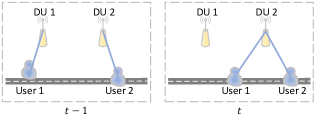
(a) User association at time steps $t$ and $t-1$, where the lines indicate the association relationships.

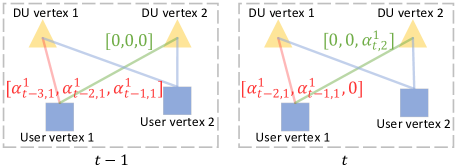
(b) State graphs at time steps $t$ and $t-1$, where the lines indicate the edges and the vectors beside the lines are the features of the edges.

Figure 1: User 1 is associated with DU 1 at time steps $t-3$, $t-2$, $t-1$ and with DU 2 at time step $t$. In the state graph, $T=2$.

III-C DDPG framework for Link Scheduling

The DRL framework for this policy is easy to establish. The duration of a time step is equal to the duration of a time slot. Each episode contains a single time step.

III-C1 Matrix-based DDPG Framework

    Action: The action vector in the $j$th time step is ${\bm{\rho}}_{j}=[\rho_{j}^{1},\cdots,\rho_{j}^{K}]^{\mathsf{T}}$. The actor network first outputs a relaxed action ${\tilde{\bm{\rho}}}_{j}=[{\tilde{\rho}}_{j}^{1},\cdots,{\tilde{\rho}}_{j}^{K}]^{\mathsf{T}},{\tilde{\rho}}_{j}^{k}\in[0,1],\forall k$, and then is followed by a function $\psi(x;\xi)$ to quantize ${\tilde{\bm{\rho}}}_{j}$ into ${\bm{\rho}}_{j}$, where $\psi(x;\xi)=0$ if $x<\xi$ and $\psi(x;\xi)=1$ otherwise. We use ${\tilde{\bm{\rho}}}_{j}$ for training and ${\bm{\rho}}_{j}$ for inference.

State: The state in the $j$th time step is the channel matrix in the $j$th time step, denoted as ${\bf H}_{j}$, whose element in the $k$th row and $m$th column is $|h_{j,m}^{k}|^{2}$.

Reward: The reward is $r_{j}=\sum_{k=1}^{K}{\tilde{R}}_{j}^{k}+\eta_{1}\sum_{k=1}^{K}\log({\tilde{\rho}}_{j}^{k})+\eta_{2}\sum_{k=1}^{K}\log(1-{\tilde{\rho}}_{j}^{k})$, where ${\tilde{R}}_{j}^{k}$ is the achieved data rate of the $k$th transceiver pair by taking the relaxed action ${\tilde{\bm{\rho}}}_{j}$, and $\eta_{1}$ and $\eta_{2}$ are hyper-parameters. The second and third terms are used to avoid the learning process converging to local optima that incurs unacceptable performance [15].

III-C2 Graph-based DDPG Framework

As stated at the beginning of this section, only the actor network is necessary for the link scheduling problem to learn the mapping from state into action. Hence, only the state graph needs to be defined.

Obtain Adjacency Matrix: Since the number of transceiver pairs remains unchanged, the graph for this problem is topology-fixed, hence the adjacency matrix is a constant. The state and action involve two types of entities: transmitter and receiver, which are respectively denoted as ${\rm tx}$ and ${\rm rx}$ for short. We define each ${\rm tx}$ as a vertex and each ${\rm rx}$ as another type of vertex. To unify the notations, we still use ${\mathcal{V}}=\{1,\cdots,2K\}$ to represent vertex set, where $1,\cdots,K$ are the indices of ${\rm tx}$ vertices, and $K+1,\cdots,2K$ are the indices of ${\rm rx}$ vertices. Since there exists either a communication link or an interference link between ${\rm tx}$ and ${\rm rx}$, there is an edge between each ${\rm tx}$ vertex and each ${\rm rx}$ vertex, and there are two types of edges: communication edge (called ${\rm com}$ edge for short) and interference edge (called ${\rm inf}$ edge for short). Then, the edge set is ${\mathcal{E}}=\{\{v_{1},v_{2}\}|v_{1}=1,\cdots,K,v_{2}=K+1,\cdots,2K\}$. Denote the adjacency matrix as ${\bf A}_{\rm D2D}$, whose element in the $i$th row and $j$th column is a non-zero integer if $\{i,j\}\in{\mathcal{E}}$, and is 0 otherwise. We set the non-zero integer as 1 for ${\rm com}$ edge and 2 for ${\rm inf}$ edge.

Obtain Feature Matrix: Each element in the state matrix is the channel gain between a ${\rm tx}$ and a ${\rm rx}$, and hence can be transformed into the feature of the edge between the two vertices. We still use ${\bf E}_{j}$ to denote the feature matrix of all edges in the state graph at time step $j$. The element in the $k$th row and $m$th column of ${\bf E}_{j}$ is ${e}_{j,m}^{k}=|h_{j,m}^{k}|^{2}$, which is the feature of the edge between the $m$th ${\rm tx}$ vertex and the $k$th ${\rm rx}$ vertex. Both ${\rm tx}$ and ${\rm rx}$ vertices do not have features.

Finally, the state graph can be expressed as

$$S^{G}_{j}=({{\bf E}_{j}},{\bf A}_{\rm D2D}).$$ (8)

IV Graph DDPG Algorithm with Desired Permutation Properties

In this section, we first propose a general method for designing GNNs with desired permutation properties. Then, we apply the method to design the graph DDPG algorithm that satisfies the permutation properties of the policy function and action-value function defined on the graphs for the two problems.

IV-A A General Method of Designing GNNs with Desired Permutation Properties

We start by introducing several permutation properties to be used in the sequel and a flexible GNN for learning the representations of vertices.

Permutation Properties: Denote $\bm{\Pi}_{1}$ and $\bm{\Pi}_{2}$ as permutation matrices. A multivariate function ${\bf y}=f({\bf X})$ is one-dimension (1D)-PE to $\bf X$ if $\bm{\Pi}_{1}{\bf y}=f(\bm{\Pi}_{1}{\bf X})$, 1D-PI to $\bf X$ if ${\bf y}=f(\bm{\Pi}_{1}{\bf X})$, two-dimension (2D)-PE to $\bf X$ if $\bm{\Pi}_{1}{\bf y}=f(\bm{\Pi}_{1}{\bf X}\bm{\Pi}_{2}^{\mathsf{T}})$, 2D-PI to $\bf X$ if ${\bf y}=f(\bm{\Pi}_{1}{\bf X}\bm{\Pi}_{2}^{\mathsf{T}})$, joint-PE to $\bf X$ if $\bm{\Pi}_{1}{\bf y}=f(\bm{\Pi}_{1}{\bf X}\bm{\Pi}_{1}^{\mathsf{T}})$, and joint-PI to $\bf X$ if ${\bf y}=f(\bm{\Pi}_{1}{\bf X}\bm{\Pi}_{1}^{\mathsf{T}})$ [12, 35].

A Flexible GNN: The permutation property of a GNN or a function defined on a graph comes from the fact that the vertices with the same type in the graph do not have ordering. Therefore, a GNN for learning a function over a graph should exhibit the same permutation property as the function defined on the graph, which needs a judicious design. In order to introduce the general method for designing a GNN with matched permutation property to a function, we first present a flexible GNN, where the processor, pooling function and combiner differ for updating the hidden representations of different vertices. In the GNN, the hidden representation of each vertex in each layer can be obtained by aggregating the processed information of each neighboring vertex and edge and combining as follows, where the neighboring vertices of a vertex are the vertices connected to the vertex with an edge, and the edge is called the neighboring edge of the vertex.

Aggregation: The aggregated output at the $v$th vertex in the $l$th layer is,

$$\small{\bf d}_{v}^{{}^{\prime}(l)}={\rm PL}_{v,n\in\mathcal{N}(v)}\left(q_{v,n}({\bf d}_{n}^{(l-1)},{\bf e}_{v}^{n};{\bm{\phi}}_{v,n}^{(l)})\right),$$ (9)

where ${\rm PL}_{v,n\in\mathcal{N}(v)}(\cdot)$ is the pooling function of the $v$th vertex to aggregate information from vertices in $\mathcal{N}(v)$ and the corresponding neighboring edges, $q_{v,n}(\cdot,\cdot;{\bm{\phi}}_{v,n}^{(l)})$ is the processor with model parameters ${\bm{\phi}}_{v,n}^{(l)}$, $\mathcal{N}(v)$ is the set of neighboring vertices of the $v$th vertex that can be obtained from adjacency matrix, ${\bf d}_{n}^{(l-1)}$ is the representation of the $n$th vertex in the $(l-1)$th layer, and ${\bf e}_{v}^{n}$ is the feature of the edge between the $v$th vertex and the $n$th vertex.

Combination: The hidden representation of the $v$th vertex in the $l$th layer is

$$\small{\bf d}_{v}^{(l)}={\rm CB}_{v}({\bf d}_{v}^{(l-1)},{\bf d}_{v}^{{}^{\prime}(l)};{\bm{\theta}}_{v}^{(l)}),$$ (10)

where ${\rm CB}_{v}(\cdot,\cdot,{\bm{\theta}}_{v}^{(l)})$ is the combiner of the $v$th vertex with model parameters ${\bm{\theta}}_{v}^{(l)}$.

When we re-order the vertices with the same type in a graph (i.e., permute the indices of these vertices), the feature matrices and adjacency matrix are permuted accordingly, while the graph topology remains unchanged. If a GNN is unaware of such a topology-invariant-with-permutation prior, the GNN will treat permuted graphs as different samples. To improve sample efficiency, this prior should be embedded in a GNN by designing the GNN to satisfy the following property.

Property 1: When the indices of the vertices with same type in a graph are permuted, the representations of these vertices learned by a GNN over the graph are permuted accordingly.

To help understand the property, we take the state graph constructed for the predictive power allocation problem with two user vertices (called Alice and Bob) as an example. The two user vertices do not have ordering, hence either Alice or Bob can be denoted as user vertex 1. Denote the vector representation of the user vertices learned by a GNN with $L$ layers over the graph in Fig. 2(a) as $[{\bf d}_{{\rm Alice}}^{(L)},{\bf d}_{{\rm Bob}}^{(L)}]^{\mathsf{T}}$. When we re-order the user vertices as in Fig. 2(b), the output of the GNN should be $[{\bf d}_{{\rm Bob}}^{(L)},{\bf d}_{{\rm Alice}}^{(L)}]^{\mathsf{T}}$ to satisfy the property.

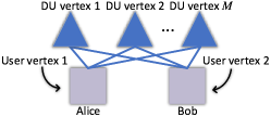
(a) Assign Alice as user vertex 1.

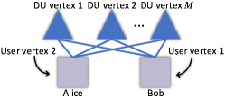
(b) Assign Bob as user vertex 1.

Figure 2: Permute the indices of two user vertices in a state graph constructed for the predictive power allocation problem.

To satisfy the permutation properties of a target function defined on graph, the GNN learning over the graph should satisfy Property 1.

Existing works either first design a GNN for learning a specific target function and then prove that the GNN can satisfy the permutation property of the function without explaining how the GNN is designed [16, 11, 20, 17, 18, 12], or design parameter sharing for a GNN to match with the permutation property of the function [35]. However, designing parameter sharing for GNNs is rather complicated when there are multiple types of vertices and edges in graphs. In the following proposition, we provide the conditions for a GNN to satisfy Property 1.

Proposition 1

A GNN will satisfy Property 1 if the three functions in (9) and (10) satisfy the following conditions: (1) $q_{v_{1},n_{1}}(\cdot)$ and $q_{v_{2},n_{2}}(\cdot)$ are identical if (i) the $v_{1}$th and the $v_{2}$th vertices are with the same type, (ii) the $n_{1}$th and the $n_{2}$th vertices are with the same type, and (iii) edge $\{v_{1},n_{1}\}$ and edge $\{v_{2},n_{2}\}$ are with the same type, (2) both ${\rm CB}_{v}(\cdot)$ and ${\rm PL}_{v,n\in\mathcal{N}(v)}(\cdot)$ are identical for the vertices with the same type, and (3) ${\rm PL}_{v,n\in\mathcal{N}(v)}(\cdot)~{}\forall v$ satisfies commutative law.

Proof:

See Appendix A. ∎

The method of designing a GNN with desired permutation properties is selecting the three functions to satisfy the conditions in the proposition, which is not task-specific.

IV-B Graph DDPG Algorithm with Desired Permutation Properties

Denote the policy function as $\mu(\cdot)$, and the action-value function as $Q(\cdot)$, both are with permutation properties determined by the graphs that the functions are defined on.

The policy function (or the action-value function) can be learned with a composite of a GNN (denoted as ${\rm GNN}(\cdot;{\bm{\theta}})$) and an output layer (denoted as $F(\cdot;{\bm{\theta}}_{f})$), which is expressed as $F({\rm GNN}(\cdot;{\bm{\theta}});{\bm{\theta}}_{f})$, where ${\bm{\theta}}$ and ${\bm{\theta}}_{f}$ are model parameters. The GNN is used to learn the vertex representation, and the output layer (also called readout layer in literature) plays the role of mapping the vertex representation into the action or expected return.

To satisfy the permutation properties of the policy function or the action-value function, both the GNN and the output layer need to be designed.

IV-C Graph DDPG Algorithm for Predictive Power Allocation

IV-C1 Desired Permutation Properties

The policy function defined on the state graph in (7) is ${\bf a}_{t}=\mu({{{\bf U}_{t}},{{\bf E}_{t}}},{\bf A}_{\rm PRA})$. If we re-order the user vertices in the state graph, then the elements in ${\bf a}_{t}$, the rows of ${\bf U}_{t}$ and ${\bf E}_{t}$, the first $K$ rows and columns of ${\bf A}_{\rm PRA}$ will be permuted. If we re-order the DU vertices, then the columns of ${\bf E}_{t}$, the last $M$ rows and columns of ${\bf A}_{\rm PRA}$ will be permuted. The action-value function defined on the state-action graph in (7) is $q=Q({{\bf{\widetilde{U}}}_{t}}$, ${{\bf E}_{t}},{\bf A}_{\rm PRA})$, where $q\triangleq\mathbb{E}[\sum_{i=t}^{(N_{v}-1)N_{f}}\gamma r_{i}]$ is the expected return and $\gamma$ is the discount factor. The value of $q$ will remain unchanged if we re-order the user or DU vertices.

Hence, the permutation properties of $\mu(\cdot)$ and $Q(\cdot)$ can be respectively expressed as

$$\small\bm{\Pi}_{1}{\bf a}_{t} =\mu(\bm{\Pi}_{1}{{\bf U}_{t}},\bm{\Pi}_{1}{{\bf E}_{t}}{\bm{\Pi}_{2}^{\mathsf{T}}},{\tilde{\bm{\Pi}}}_{1}{\bf A}_{\rm PRA}{\tilde{\bm{\Pi}}}_{1}^{\mathsf{T}}),$$ (11a)

$$q =Q({\bm{\Pi}_{1}{{\bf{\widetilde{U}}}_{t}},\bm{\Pi}_{1}{{\bf E}_{t}}{\bm{\Pi}_{2}^{\mathsf{T}}},{\tilde{\bm{\Pi}}}_{1}{\bf A}_{\rm PRA}{\tilde{\bm{\Pi}}}_{1}^{\mathsf{T}}}),$$ (11b)

where ${\tilde{\bm{\Pi}}}_{1}={\rm diag}({\bm{\Pi}_{1}},{\bm{\Pi}_{2}})$ is a block diagonal matrix, ${\bm{\Pi}_{1}}\in\mathbb{I}^{K\times K}$ and ${\bm{\Pi}_{2}}\in\mathbb{I}^{M\times M}$ are arbitrary permutation matrices.

IV-C2 Design of GNN to Satisfy Desired Permutation Properties

There are a variety of choices for the processor, pooling function and combiner [40]. For easy understanding, we choose simple functions to show how to apply the general method for designing a GNN with desired permutation properties. In particular, we choose processor as FNN, pooling function as mean function, and combiner as a linear function followed by an activation function.

In the state graph and state-action graph in (7), there are two types of vertices (i.e., DU vertices and user vertices) and one type of edge. All user vertices are the neighbouring vertices of a DU vertex, and all DU vertices are the neighbouring vertices of a user vertex. Hence, there are two types of vertices that aggregate information, one type of neighboring vertices to be aggregated, and one type of neighboring edges between them.

To satisfy condition (1) in Proposition 1, all DU vertices aggregate information from user vertices and neighbouring edges with the same processor (denoted as ${\rm FNN}_{1}(\cdot)$), and all user vertices aggregate information from DU vertices and neighbouring edges with the same processor (denoted as ${\rm FNN}_{2}(\cdot)$).

To satisfy condition (2), all DU vertices (or all user vertices) use the same pooling function (i.e., mean function) and the same combination function. For all DU vertices, the combiner is ${\rm CB}_{v}({\bf d}_{v}^{(l-1)},{\bf d}_{v}^{{}^{\prime}(l)};{\bm{\theta}}_{v}^{(l)})=\sigma({\bf V}_{1}^{(l)}{\bf d}_{v}^{(l-1)}+{\bf d}_{v}^{{}^{\prime}(l)})$, where ${\bm{\theta}}_{v}^{(l)}=\{{\bf V}_{1}^{(l)}\}$, $v=K+1,\cdots,K+M$, and $\sigma(\cdot)$ is an activation function. For all user vertices, the combiner is ${{\rm CB}}_{v}({\bf d}_{v}^{(l-1)},{\bf d}_{v}^{{}^{\prime}(l)};{\tilde{\bm{\theta}}}_{v}^{(l)})=\sigma({\bf Y}_{1}^{(l)}{\bf d}_{v}^{(l-1)}+{\bf d}_{v}^{{}^{\prime}(l)})$, where ${\tilde{\bm{\theta}}}_{v}^{(l)}=\{{\bf Y}_{1}^{(l)}\}$, and $v=1,\cdots,K$.

The condition (3) is satisfied when the pooling function is the mean function.

For easy understanding, we replace ${\bf d}_{v}^{(l-1)}$ in (9) and (10) by ${\bf b}_{t,m}^{(l-1)}$ and ${\bf u}_{t,k}^{(l-1)}$, which respectively denote the hidden representations of the $m$th DU vertex and the $k$th user vertex in the $(l-1)$th layer at time step $t$, and replace ${\bf e}_{v}^{n}$ in (9) and (10) by ${\bf e}_{t,m}^{k}$, which denotes the feature of the edge between the $m$th DU vertex and the $k$th user vertex at time step $t$. We add subscript $t$ due to the time-varying feature matrices of the state graph and the state-action graph in (7).

Then, the update equation of the GNN for predictive power allocation problem becomes,

DU vertices aggregating information from user vertices

$${\sf{Aggregation}}:{\bf b^{\prime}}_{t,m}^{(l)}=\frac{1}{K}\sum\nolimits_{k=1}^{K}{\rm FNN}_{1}({\bf u}_{t,k}^{(l-1)},{\bf e}_{t,m}^{k}),$$

$${\sf{Combination}}:{\bf b}_{t,m}^{(l)}=\sigma\left({\bf V}_{1}^{(l)}{\bf b}_{t,m}^{(l-1)}+{\bf b^{\prime}}_{t,m}^{(l)}\right),m=1\cdots,M,$$ (12a)

User vertices aggregating information from DU vertices

$${\sf{Aggregation}}:{\bf u^{\prime}}_{t,k}^{(l)}=\frac{1}{M}\sum\nolimits_{m=1}^{M}{\rm FNN}_{2}({\bf b}_{t,m}^{(l-1)},{\bf e}_{t,m}^{k}),$$

$${\sf{Combination}}:{\bf u}_{t,k}^{(l)}=\sigma\left({\bf Y}_{1}^{(l)}{\bf u}_{t,k}^{(l-1)}+{\bf u^{\prime}}_{t,k}^{(l)}\right),k=1\cdots,K,$$ (12b)

where ${\bf b}_{t,m}^{(0)}=0,\forall t,m$, since DU vertices have no features.

The update equation can be applied for both actor and critic networks, where the input of the actor network is state graph, and the input of the critic network is state-action graph. We denote the outputs of both networks as ${\bf U}_{t}^{(L)}\triangleq[{\bf u}_{t,1}^{(L)},\cdots,{\bf u}_{t,K}^{(L)}]^{\mathsf{T}}$ and ${\bf B}_{t}^{(L)}\triangleq[{\bf b}_{t,1}^{(L)},\cdots,{\bf b}_{t,M}^{(L)}]^{\mathsf{T}}$.

Remark 2

In (12), each user or DU vertex aggregates information from neighboring DU or user vertices. This is because the features of edges between user and DU vertices contain the historical channels that are useful for predictive power allocation, as explained in Remark 1.

IV-C3 Design of Output Layer to Satisfy Desired Permutation Properties

For the actor network, if we re-order the user vertices in the state graph, ${\bf U}_{t}^{(L)}$ will be permuted to ${\bm{\Pi}}_{1}{\bf U}_{t}^{(L)}$, since the GNN with update equation in (12) satisfies Property 1. To satisfy the permutation property of the policy function in (11a), the learned action ${\bf a}_{t}$ should be 1D-PE to ${\bf U}_{t}^{(L)}$ and 1D-PI to ${\bf B}_{t}^{(L)}$. Hence, the output layer should satisfy the following property, ${{\bm{\Pi}}_{1}}{\bf a}_{t}=F({\bm{\Pi}}_{1}{\bf U}_{t}^{(L)},{\bm{\Pi}}_{2}{\bf B}_{t}^{(L)})$. Considering that the output layer satisfying this property is not unique, we select a simple one, i.e., ${\bf a}_{t}=F({\bf U}_{t}^{(L)},{\bf B}_{t}^{(L)})={\bf U}_{t}^{(L)}$. Since ${\bf a}_{t}$ is a vector but ${\bf U}_{t}^{(L)}$ is a matrix, all dimensions of ${\bf u}_{t,1}^{(L)},\cdots,{\bf u}_{t,K}^{(L)}$ should be set as one.

For the critic network, if we re-order the user and DU vertices in the state-action graph, ${\bf U}_{t}^{(L)}$ and ${\bf B}_{t}^{(L)}$ are respectively permuted to ${\bm{\Pi}}_{1}{\bf U}_{t}^{(L)}$ and ${\bm{\Pi}}_{2}{\bf B}_{t}^{(L)}$. To satisfy the permutation property of the action-value function in (11b), the output layer should satisfy the following property, $q=F({\bm{\Pi}}_{1}{\bf U}_{t}^{(L)},{\bm{\Pi}}_{2}{\bf B}_{t}^{(L)})$. Again, we select a simple function that satisfies the property, which is $q=\lambda_{1}\sum_{k=1}^{K}{{\bf u}_{t,k}^{(L)}}+\lambda_{2}\sum_{m=1}^{M}{{\bf b}_{t,m}^{(L)}}$, where $\lambda_{1}$ and $\lambda_{2}$ are hyper-parameters. Since $q$ is a scalar, the dimension of every vector ${\bf u}_{t,1}^{(L)},\cdots,{\bf u}_{t,K}^{(L)},{\bf b}_{t,1}^{(L)},\cdots,{\bf b}_{t,M}^{(L)}$ should be set as one.

IV-D Graph DDPG Algorithm for Link Scheduling

IV-D1 Desired Permutation Properties

The policy function is ${\bm{\rho}}_{j}=\mu({\bf E}_{j},$ ${\bf A}_{\rm D2D})$. It is easy to see that $\mu(\cdot)$ satisfies the following property: $\bm{\Pi}_{1}{\bm{\rho}}_{j}=\mu({\bm{\Pi}_{1}{{\bf E}_{j}}{\bm{\Pi}_{2}^{\mathsf{T}}}},$ ${\tilde{\bm{\Pi}}}_{1}{\bf A}_{\rm D2D}{\tilde{\bm{\Pi}}}_{1}^{\mathsf{T}})$.

IV-D2 Design of GNN to Satisfy Desired Permutation Properties

In the state graph in (8), there are two types of vertices ($\rm tx$ and $\rm rx$ vertices) and two types of edges ($\rm com$ and $\rm inf$ edges). All $\rm tx$ vertices are the neighbouring vertices of a $\rm rx$ vertex, and all $\rm rx$ vertices are the neighbouring vertices of a $\rm tx$ vertex. There are two types of vertices that aggregate information, one type of neighboring vertices to be aggregated, and two types of the neighboring edges between them.

To satisfy condition (1) in Proposition 1, four processors are respectively required for (i) $\rm tx$ vertex aggregating information from $\rm rx$ vertex and $\rm com$ edge with $\rm FNN_{3}(\cdot)$, (ii) $\rm tx$ vertex aggregating information from $\rm rx$ vertex and $\rm inf$ edge with $\rm FNN_{4}(\cdot)$, (iii) $\rm rx$ vertex aggregating information from $\rm tx$ vertex and $\rm com$ edge with $\rm FNN_{5}(\cdot)$, and (iv) $\rm rx$ vertex aggregating information from $\rm tx$ vertex and $\rm inf$ edge with $\rm FNN_{6}(\cdot)$.

To satisfy conditions (2) and (3), all $\rm tx$ vertices or all $\rm rx$ vertices use the same pooling function and combiner, which are again selected as a mean function and a linear function followed by an activation function. We still use ${\bf b}_{j,m}^{(l-1)}$ and ${\bf u}_{j,k}^{(l-1)}$ to respectively denote the outputs of the $m$th $\rm tx$ vertex and the $k$th $\rm rx$ vertex in the $(l-1)$th layer at time step $j$.

Then, the update equation of the designed GNN can be expressed as follows,

Tx vertices aggregating information from rx vertices

$${\sf{Aggregation}}:{\bf b^{\prime}}_{j,m}^{(l)}=\frac{1}{K}\left({\rm FNN_{3}}({\bf u}_{j,m}^{(l-1)},{\bf e}_{j,m}^{m})+\sum\nolimits_{k=1,k\neq m}^{K}{\rm FNN_{4}}({\bf u}_{j,k}^{(l-1)},{\bf e}_{j,m}^{k})\right),$$

$${\sf{Combination}}:{\bf b}_{j,m}^{(l)}=\sigma\left({\bf V}_{2}^{(l)}{\bf b}_{j,m}^{(l-1)}+{\bf b^{\prime}}_{j,m}^{(l)}\right),m=1\cdots,K,$$ (13a)

Rx vertices aggregating information from tx vertices

$${\sf{Aggregation}}:{\bf u^{\prime}}_{j,k}^{(l)}=\frac{1}{K}\left({\rm FNN_{5}}({\bf b}_{j,k}^{(l-1)},{\bf e}_{j,k}^{k})+\sum\nolimits_{m=1,m\neq k}^{K}{\rm FNN_{6}}({\bf b}_{j,m}^{(l-1)},{\bf e}_{j,m}^{k})\right),$$

$${\sf{Combination}}:{\bf u}_{j,k}^{(l)}=\sigma\left({\bf Y}_{2}^{(l)}{\bf u}_{j,k}^{(l-1)}+{\bf u^{\prime}}_{j,k}^{(l)}\right),k=1\cdots,K,$$ (13b)

where ${\bf b}_{j,m}^{(0)}=0,\forall j,m$, and ${\bf u}_{j,k}^{(0)}=0,\forall j,k$, since both $\rm rx$ and $\rm tx$ vertices have no features.

Denote the outputs of the GNN as ${\bf B}_{j}^{(L)}=[{\bf b}_{j,1}^{(L)},\cdots,{\bf b}_{j,M}^{(L)}]^{\mathsf{T}}$ and ${\bf U}_{j}^{(L)}=[{\bf u}_{j,1}^{(L)},\cdots,{\bf u}_{j,K}^{(L)}]^{\mathsf{T}}$.

IV-D3 Design of Output Layer to Satisfy Desired Permutation Properties

To satisfy the permutation property of the policy function for optimizing link scheduling, the output layer should satisfy ${\bm{\Pi}}_{1}{\tilde{\bm{\rho}}}_{j}=F({\bm{\Pi}}_{1}{\bf B}_{j}^{(L)},{\bm{\Pi}}_{2}{\bf U}_{j}^{(L)})$. We select the output layer as ${\tilde{\bm{\rho}}}_{j}=F({\bf B}_{j}^{(L)},{\bf U}_{j}^{(L)})={\bf B}_{j}^{(L)}$, and set the dimension of every vector ${\bf b}_{j,1}^{(L)},\cdots,{\bf b}_{j,M}^{(L)}$ as one.

IV-E Time Complexity of Graph-based and Matrix-based DDPG Algorithms

In order for adapting to dynamic environments, a DRL algorithm is trained online, which continually updates the DNNs by interacting with environment as follows. (i) In each time step, the agent observes a state, and executes an action with the actor network (i.e., inference). Then, the agent computes the reward and observes a new state after taking the action, and stores the state, action, reward and the new state as an experience in a replay buffer. (ii) The agent selects a batch of experiences and updates the DNNs (i.e., training) every several time steps.

In the following, we analyze the time complexity of the graph-based DDPG (GNN-DDPG for short) and matrix-based DDPG (FNN-DDPG for short) algorithms for inference and training, by taking those for predictive power allocation as an example. The FNN-DDPG uses two FNNs to learn the policy and action-value functions, where the matrix-based DDPG framework in section III-B1 is used. We analyze the number of multiplications, which is the most commonly used metric for the time complexity of neural networks.

Suppose that both the actor and critic networks have $L$ layers. For the GNN-DDPG, the dimension of the hidden representation of each vertex in each layer is $d$, the dimension of the feature vector of each edge (i.e., ${\bf e}_{t,m}^{k}\in\mathbb{R}^{(T+1)\times 1}$) is $(T+1)$. For the FNN-DDPG, the dimension of the hidden output of each layer is $D$. The batch size is $B$.

To simplify the expressions of the time complexity, we replace ${\rm FNN}_{1}(\cdot)$ and ${\rm FNN}_{2}(\cdot)$ in (12) as linear processors. Then, the time complexity for inference with the GNN-DDPG can be derived as $\mathcal{O}(MKLd^{2})$, and that with the FNN-DDPG is $\mathcal{O}(LD^{2})$. By further counting the number of multiplications used for computing the gradient with respect to every model parameter matrices in every layer, the time complexity for training the GNNs once is $\mathcal{O}[(MK^{2}+M^{2}K)BLd^{2})]$ and for training the FNNs once is $\mathcal{O}(BLD^{2})$.

V Simulation Results

In this section, we evaluate the performance of the resource allocation of the two problems learned by the graph DDPG algorithms.

V-A Predictive Power Allocation for Video Streaming

We compare the proposed method (with legend “GNN-DDPG”) designed in sections IV-C and III-B2 that optimizes predictive rate allocation in each frame using graph DDPG algorithm and optimizes the power allocation in each time slot using $\pi_{{\rm P}3}(\cdot;{\bm{\phi}})$ with the following methods.

“Optimal”: This method uses the numerical algorithm in [31] to find the optimal power allocation from ${\rm P}1$ by assuming perfect future large-scale channel gains, which can serve as the performance upper bound for all the learning-based solutions.

“Non-predictive”: This is a traditional method of transmission without using predicted information, which maintains a constant average rate for each user in each frame [27]. To satisfy the QoS constraints, the average rate for the $k$th user in the $t$th frame is set as ${\bar{R}}_{t}^{k}=d_{n_{t}+1}^{k}/(N_{f}\Delta T)$, where $n_{t}$ is the index of the segment played in the $t$th frame, and $d_{n_{t}+1}^{k}$ is the number of bits of the $(n_{t}+1)$th segment in the video to be played by the $k$th user. For a fair comparison, the power allocation in each time slot is obtained with $\pi_{{\rm P}3}(\cdot;{\bm{\phi}})$.

“LSTM & Optimize”: This method solves problem ${\rm P}2$ by treating the predicted large-scale channels as the real channels [14]. The large-scale channel gains in future $(N_{v}-1)N_{f}$ frames are first predicted with a long short-term memory network (LSTM), with which the future powers are obtained with the numerical optimization algorithm in [31].

“GNN-DDPG+FNN”: This DRL algorithm differs from “GNN-DDPG” only in the output layers, which are FNNs analogous to the graph DQN in [23]. Hence, the actor and critic networks do not satisfy the PE/PI properties in (11).

“FNN-DDPG”: This is the DRL algorithm mentioned in section IV-E. The actor and critic networks do not satisfy the PE/PI properties in (11).

“PE/PINN-DDPG”: The only difference of this DRL algorithm from “FNN-DDPG” is that the two FNNs are replaced by PE/PINNs that satisfy the PE/PI properties in (11) using the method in [35]. Hence, the permutation prior is exploited but the topology prior is not harnessed.

V-A1 Simulation Setup

Consider a scenario shown in Fig. 3, where $K$ users move along roads across cells. The trajectory of each user is generated with Bonnmotion software [41], which is commonly applied for vehicular networks, where the trajectory follows Gauss-Markov model. The initial velocity of the users is set as 16 m/s, and the minimal and maximal velocities are 12 m/s and 20 m/s, respectively. When a user encounters a traffic light, which is red or green with 50% probability, the user stops 0 $\sim$ 30 seconds if the traffic light is red.

The playback duration of each video and each segment are 150 s and 10 s, respectively. Each segment is with size of $8$ Mbps. Each time frame is with duration of $\Delta T=1$ s, and each time slot is with duration of $\tau=1$ ms (i.e., $N_{s}=1000$).

The maximal transmit power and the number of antennas of each DU are 200 W and 64, respectively. The bandwidth assigned for each user is 2 MHz. The path loss is modeled as $13.54+39.08\log_{10}(d)+20\log_{10}(f_{c})$ in dB, where $d$ is the distance between user and DU in meters, $f_{c}$ is the carrier frequency and is set as 3.5 GHz [42]. The small-scale channels follow Rayleigh fading. The noise spectral density is -174 dBm/Hz.

The simulation setup is used in the following unless otherwise specified.

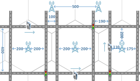
Figure 3: Simulation scenario, where $K$ users move along roads in five cells, and the integers indicate distance in meters.

V-A2 Fine-Tuned Parameters

We set $T=2$ in the state, and $\lambda=0.1$ in the reward. The discount factor $\gamma=1$. The replay memory size is $10^{6}$, and the mini-batch size for gradient descent is 1024. The noise term for exploration follows Gaussian distribution with zero mean and variance decreased linearly from $0.1$ to $0$. We use Adam algorithm [43] to optimize the model parameters. For “GNN-DDPG”, we set $\lambda_{1}=1$ and $\lambda_{2}=0$ in the critic network. Other fine-tuned hyper-parameters are listed in Table I.

We extend the batch normalization method [44] to heterogeneous graphs, where the normalization is conducted for the hidden representations of each type of vertices independently. In particular, consider a batch of graphs $\{G_{1},\cdots,G_{{B}}\}$, where ${B}$ is the batch size. Denote $\mathcal{A}_{g}^{a}$ as the index set of vertices in graph $G_{g}$ that belong to the $a$th type. Then, the $i$th feature of the $j$th vertex ($j\in\mathcal{A}_{g}^{a}$) in graph $G_{g}$, denoted as $h_{i,j,g}$, can be normalized as ${\rm Norm}(h_{i,j,g})=\beta_{1}\frac{h_{i,j,g}-\mu}{\sigma}+\beta_{2}$, where $\mu=\frac{\sum_{g=1}^{{B}}\sum\nolimits_{j\in\mathcal{A}_{g}^{a}}h_{i,j,g}}{{B}\cdot\sum_{g=1}^{G}|\mathcal{A}_{g}^{a}|}$, $\sigma=\frac{\sum_{g=1}^{\mathcal{B}}\sum\nolimits_{j\in\mathcal{A}_{g}^{a}}(h_{i,j,g}-\mu)^{2}}{{B}\cdot\sum_{g=1}^{G}|\mathcal{A}_{g}^{a}|}$, $\beta_{1}$ and $\beta_{2}$ are parameters that need to be trained, and $|\cdot|$ denotes the cardinality of a set.

TABLE I: Hyper-Parameters of each DRL algorithm.

		FNN-   DDPG	GNN-DDPG	GNN-DDPG       +FNN	PE/PINN  -DDPG
Learning rate of actor network		0.001	0.001	0.001	0.001
Learning rate of critic network		0.0001	0.0001	0.001	0.0001
Number of neurons in each layer and number of layers	$K=2$	$[200,200]^{*}$	$[128,128]^{**}$	[128, 128], [500]	[200, 200]
	$K=5$	[400, 400, 400]	[128, 128]	[128, 128], [500]	[400, 400]
	$K=8$	[600, 600, 600]	[128, 128]	[128, 128], [500]	[800, 800, 800]

• $*_{1}$ and $*_{2}$ in $[*_{1},*_{2},\cdots]$ indicate the number of neurons in the first and second layers of a neural network, respectively.

• The listed number of neurons in the hidden layer of GNN is the dimension of the hidden representation of each vertex, and the number of neurons in the hidden layer of FNN is the dimension of the output vector of the whole layer.

V-A3 Performance Evaluation

In Fig. 4, we show the learning curves of the DRL algorithms. The negative return is the total energy consumed at the DUs of all users by a learned policy. The shadow near each curve is the maximal and minimal returns of the 10 times of training. As shown in Fig. 4(a), the convergence speed of “GNN-DDPG” is faster than all the other algorithms. Owing to not satisfying the permutation properties, “GNN-DDPG+FNN” converges much slower than “GNN-DDPG” and only converges slightly faster than “FNN-DDPG”. Since “PE/PINN-DDPG” does not exploit the relational prior among vertices, it converges slower than “GNN-DDPG”. Due to not using future information, “Non-predictive” is inferior to all the DRL algorithms that can predict channels implicitly by including historical channels in the states. Due to the large prediction errors in the multi-step prediction, “LSTM & Optimize” is also inferior to all the DRL algorithms that are with an implicit single-step prediction. After convergence, none of the DRL algorithms can achieve the upper bound provided by “Optimal”. This is due to the randomly generated trajectories, including the random initial locations of users, random velocities, random turn in crossing and random stopping time for red traffic lights that are unpredictable. We also compare with other DDPG algorithms in Fig. 4(b), where the actor and critic networks are the GNNs designed in [11] and [16], which perform worse due to the unmatched permutation properties with (11a) and (11b).

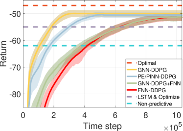
(a) Impact of two relational priors and channel prediction

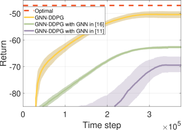
(b) Impact of GNNs with unmatched permutation properties

Figure 4: Negative energy consumption $\sim$ time steps, averaged over 10 Monte Carlo trials and 100 successive episodes, $K=5$.

In Fig. 5, we show the scalability of several DDPG algorithms, which are trained for each value of $K$. The results for different number of users are obtained after convergence (the numbers of required time steps are shown on the top of the bars). Since the performance upper bound and the return depend on channels and number of users, to compare the algorithms in different setups, we consider the performance loss from the upper bound, defined as $|\frac{|\text{Return}_{c}|-\text{Energy}_{op}}{\text{Energy}_{op}}|$, where $\text{Return}_{c}$ is the return achieved by the DDPG algorithms after convergence, and $\text{Energy}_{op}$ is the energy achieved by “Optimal”. Since training “FNN-DDPG” and “PE/PINN-DDPG” is too time-consuming, their performance losses for $K>10$ are not provided. We can see that the performance losses of “GNN-DDPG” and “PE/PINN-DDPG” remain unchanged when $K$ increases (i.e., they are scalable), but “FNN-DDPG” performs much worse for more users even with significantly more time steps than “GNN-DDPG”. We also evaluated the scalability of the DDPG algorithms to the number of DUs (with retraining) and the generalizability of them to the unseen number of users (without retraining). The results show that both “GNN-DDPG” and “PE/PINN-DDPG” are generalizable to $K$ but “FNN-DDPG” cannot. Both “GNN-DDPG” and “PE/PINN-DDPG” are scalable but all the three DDPG algorithms are not generalizable to the number of DUs. The results are not provided due to the space limitation.

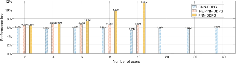
Figure 5: Scalability of DDPG algorithms, averaged over Monte Carlo trials.

In Table II, we compare the training complexity of several DDPG algorithms, which is obtained on a computer with Intel CoreTM i9-10940X CPU (3.30GHz) and NVIDIA GeForce RTX 3080 GPU. Sample complexity is the minimal number of experiences required for converging to an expected performance. Space complexity and time complexity are respectively the number of free parameters in the fine-tuned DNNs and the running time (in seconds) for updating the DNNs once of each DDPG algorithm. We can see that the gain of exploiting relational priors in terms of reducing sample and space complexities is large when $K=8$. In particular, “GNN-DDPG” converges 12 times faster than “FNN-DDPG”, and five times faster than “PE/PINN-DDPG”.

TABLE II: Training Complexity of the DDPG algorithms when converging to 10% performance loss.

	FNN- DDPG	GNN-DDPG	GNN-DDPG +FNN	PE/PINN -DDPG	FNN- DDPG	GNN-DDPG	GNN-DDPG +FNN	PE/PINN -DDPG
$K$	2				8
Sample complexity	0.84M	0.36M	0.84M	0.72M	6.00M	0.48M	4.32M	2.40M
Space complexity	178K	401K	914K	90K	3092K	401K	2456K	169K
Time complexity	0.010	0.026	0.022	0.012	0.020	0.029	0.032	0.031

V-B Link Scheduling for D2D Communications

We compare the proposed method (with legend “GNN-DDPG” designed in sections IV-D and III-C2 with the following methods.

“FPLinQ”: This method uses the numerical algorithm in [34] to solve the problem in (2).

“FNN-DDPG”: This method differs from GNN-DDPG only in the DNN for learning the policy function, which uses a FNN as the actor network under the framework in section III-C1.

“HomoGNN-DDPG”: This method differs from GNN-DDPG only in the GNN, where the homogeneous GNN designed in [16] is applied. In the GNN, the processor and combiner are two FNNs that are identical for all vertices and the pooling function is maximization.

V-B1 Simulation Setup

50 D2D pairs are randomly located in a 500 m$\times$500 m area. The distance between the transmitter and the receiver in a D2D pair is uniformly distributed in [2 m, 65 m]. We use the line-of-sight model in [45] as the channel model. The transmit power of each transmitter is 40 dBm. The noise spectral density is -169 dBm/Hz.

V-B2 Fine-Tuned Parameters

Adam algorithm [43] is used to optimize the model parameters, and the mini-batch size is 16. For “HomoGNN-DDPG” and “GNN-DDPG”, all FNNs have one hidden layer with 16 neurons. We set $\eta_{1}=0.1$ and $\eta_{2}=0.0001$ in reward. The actor network employs ${\rm sigmoid}$ as the activation function to ensure the relaxed action ${\tilde{\rho}}^{k}_{j}\in[0,1],\forall k$. Other fine-tuned hyper-parameters are listed in Table III.

TABLE III: Hyper-Parameters of each algorithm.

	FNN-DDPG	HomoGNN-DDPG	GNN-DDPG
Learning rate of actor network	0.001		0.0015
Number of neurons in each layer and number of layers	[400,400,400,50]	[8,8,8,8,8,1]

V-B3 Performance Evaluation

In Fig. 6, we show the learning curves of the DDPG algorithms. The return is the sum-rate of all D2D pairs in each time slot. We can see that “GNN-DDPG” achieves higher sum-rate and converges faster than other DDPG algorithms.

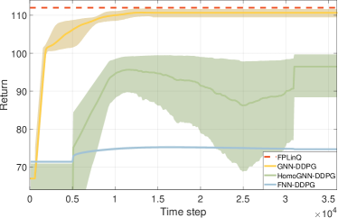
Figure 6: Sum-rate $\sim$ time steps, averaged over 5 Monte Carlo trials and 10 successive time steps, $K=50$.

VI Conclusion

In this paper, we investigated how to harness two kinds of relational priors for reducing training complexity of graph DRL frameworks. We provided a method for transforming the matrix-based DRL framework into graph-based DRL framework, and proposed a method for designing GNNs to satisfy desired permutation properties. By taking DDPG algorithm as example, we showed that the actor and critic networks can satisfy the permutation properties of the policy and action-value functions by sharing the processor, combiner and pooling functions in the GNNs and by designing the output layers. Simulation results for the predictive resource allocation and link scheduling problems showed that the designed graph-based DDPG algorithm converges much faster and needs much lower space complexity than the matrix-based DDPG algorithm, especially for more users. The proposed methods are generic, which are also applicable to deep learning and other DRL algorithms.

Appendix A: Proof of Proposition 1

Denote $n_{a}$ as the number of vertices of the $a$th type, where $a\in\mathcal{A}$ and $\mathcal{A}$ is the set of vertex types. The indices of all vertices and indices of the vertices of the $a_{1}$th type can be expressed as $\{\underbrace{1,\cdots,n_{1}}_{\text{the first type}},\underbrace{n_{1}+1,\cdots,n_{1}+n_{2}}_{\text{the second type}},\cdots,$ $\sum_{a=1}^{|\mathcal{A}|}n_{a}\}$ and ${\mathcal{N}}_{a_{1}}=\{\sum_{i=1}^{a_{1}-1}{n_{i}}+1,\cdots,\sum_{i=1}^{a_{1}}{n_{i}}\}$, respectively. Only the vertices of the same type are permutable. When we permute the vertices of the $a_{1}$th type, the indices of the vertices of this type become $\{\pi(\sum_{i=1}^{a_{1}-1}{n_{i}}+1),\cdots,\pi(\sum_{i=1}^{a_{1}}{n_{i}})\}$, where $\pi(\cdot)$ stands for the permutation operation on the elements of a set.

Recall that ${\bf d^{\prime}}_{m}^{(l)}$ and ${\bf d}_{m}^{(l)}$ are respectively the aggregation output and hidden output of the $m$th vertex in the $l$th layer. We use $\widetilde{{\bf d^{\prime}}}_{m}^{(l)}$ and $\widetilde{\bf d}_{m}^{(l)}$ to denote the aggregation output and hidden representation of the $m$th vertex in the $l$th layer when we permute the vertices of the $a_{1}$th type.

We aim to prove that

$$\footnotesize\widetilde{\bf d}_{\pi(m)}^{(L)}={\bf d}_{m}^{(L)},\quad\forall m\in\mathcal{N}_{a_{1}},$$ (A.1)

where $L$ is the number of layers of the GNN. If we can prove that

$$\footnotesize\widetilde{\bf d}_{\pi(m)}^{(l)}={\bf d}_{m}^{(l)},\quad\forall m\in\mathcal{N}_{a_{1}},$$ (A.2)

are true for $\forall l$, then (A.1) holds when $l=L$. In the sequel, we use Mathematical Induction method to prove (A.2).

When $l=0$, i.e., in the input layer, ${\bf d}_{m}^{(0)}$ is the feature of the $m$th vertex. The features of the vertices in $\mathcal{N}_{a_{1}}$ are permuted in the same way as the permutation of indices, hence (A.2) is true.

In what follows, we prove that (A.2) is true when $l=l_{0}+1$ if (A.2) is true when $l=l_{0}$. According to (9) and (10), if we do not permute the vertices of the $a_{1}$th type, the hidden representation of the $m$th vertex in the $(l_{0}+1)$th layer can be obtained as

$${\bf d^{\prime}}_{m}^{(l_{0}+1)} ={\rm PL}_{m,n\in\mathcal{N}(m)}\left(q_{m,n}({\bf d}_{n}^{(l_{0})},{\bf e}_{m}^{n};{\bm{\phi}}_{m,n}^{(l_{0}+1)})\right),$$ (A.3a)

$${\bf d}_{m}^{(l_{0}+1)} ={\rm CB}_{m}({\bf d}_{m}^{(l_{0})},{\bf d^{\prime}}_{m}^{(l_{0}+1)};{\bm{\theta}}_{m}^{(l_{0}+1)}).$$ (A.3b)

${\rm CB}_{m}(\cdot,\cdot;{\bm{\theta}}_{m}^{(l_{0}+1)})$ in (A.3b) maps ${\bf d}_{m}^{(l_{0})}$ and ${\bf d^{\prime}}_{m}^{(l_{0}+1)}$ into ${\bf d}_{m}^{(l_{0}+1)}$. If ${\rm CB}_{m}(\cdot,\cdot;{\bm{\theta}}_{m}^{(l_{0}+1)})$, ${\bf d}_{m}^{(l_{0})}$ and ${\bf d^{\prime}}_{m}^{(l_{0}+1)}$ remain unchanged when we permute the vertices of the $a_{1}$th type, then ${\bf d}_{m}^{(l_{0}+1)}$ will be unchanged. ${\rm CB}_{m}(\cdot,\cdot;{\bm{\theta}}_{m}^{(l_{0}+1)})$ remains unchanged because of the condition that the combination function is the same for all vertices with the same type. ${\bf d}_{m}^{(l_{0})}$ remains unchanged because we assume that (A.2) is true when $l=l_{0}$, i.e., $\widetilde{\bf d}_{\pi(m)}^{(l_{0})}={\bf d}_{m}^{(l_{0})}$. In the following, we prove that ${\bf d^{\prime}}_{m}^{(l_{0}+1)}$ remains unchanged when we permute the vertices of the $a_{1}$th type.

Considering that when we re-order a vertex (say the $m$th vertex is re-ordered the $\pi(m)$th vertex), its neighboring vertices of the same type and the edges connecting them are re-ordered accordingly, we have

$$\footnotesize q_{m,n}({\bf d}_{n}^{(l_{0})},{\bf e}_{m}^{n};{\bm{\phi}}_{m,n}^{(l_{0}+1)})={q}_{\pi(m),n}({\bf d}_{n}^{(l_{0})},{\bf e}_{\pi(m)}^{n};{\bm{\phi}}_{\pi(m),n}^{(l_{0}+1)}),\hskip 8.00002pt\forall m\in\mathcal{N}_{a_{1}},\forall n\in{\mathcal{\tilde{N}}}(\pi(m))$$ (A.4)

where ${\mathcal{\tilde{N}}}(\pi(m))$ is the set of neighboring vertices of the $\pi(m)$th vertex after the re-ordering.

According to the condition that the pooling function is the same for all vertices with the same type, the pooling function of the $m$th vertex and the $\pi(m)$th vertex is the same. According to (A.4), and further considering that the pooling function satisfies the commutative law, we can obtain ${\rm PL}_{m,n\in\mathcal{N}(m)}\left(q_{m,n}({\bf d}_{n}^{(l_{0})},{\bf e}_{m}^{n};{\bm{\phi}}_{m,n}^{(l_{0}+1)})\right)={\rm{PL}}_{\pi(m),n\in{\mathcal{\tilde{N}}}(\pi(m))}\left({q}_{\pi(m),n}({\bf d}_{n}^{(l_{0})},{\bf e}_{\pi(m)}^{n};{\bm{\phi}}_{\pi(m),n}^{(l_{0}+1)}))\right)$. This indicates that ${\bf d^{\prime}}_{m}^{(l_{0}+1)}$ remains unchanged when we permute the vertices of the $a_{1}$th type.

From (A.3b), we know that ${\bf d}_{m}^{(l_{0}+1)}$ remains unchanged, i.e., (A.2) is true for the $m$th vertex when $l=l_{0}+1$. Since the $m$th vertex is arbitrarily chosen from $\mathcal{N}_{a_{1}}$, the proof holds for all the vertices in $\mathcal{N}_{a_{1}}$. Therefore, (A.2) is true when $l=l_{0}+1$.

According to Mathematical Induction method, we know that (A.2) is true for $\forall l$, hence (A.1) is true when $l=L$. This completes the proof for Proposition 1.

References

- [1] Z. Zhang, Y. Yang, M. Hua et al., “Proactive caching for vehicular multi-view 3D video streaming via deep reinforcement learning,” IEEE Trans. Commun., vol. 18, no. 5, pp. 2693–2706, 2019.
- [2] J. Zhang, Y. Huang, J. Wang, and X. You, “Intelligent beam training for millimeter-wave communications via deep reinforcement learning,” IEEE GLOBECOM, 2019.
- [3] D. Liu, J. Zhao, and C. Yang, “Energy-saving predictive video streaming with deep reinforcement learning,” IEEE GLOBECOM, 2019.
- [4] A. Khan and R. Adve, “Centralized and distributed deep reinforcement learning methods for downlink sum-rate optimization,” IEEE Trans. Commun., vol. 19, no. 12, pp. 8410–8426, 2020.
- [5] K. Feng, Q. Wang, X. Li et al., “Deep reinforcement learning based intelligent reflecting surface optimization for MISO communication systems,” IEEE Wireless Commun. Lett., vol. 9, no. 5, pp. 745–749, 2020.
- [6] A. Kasgari, W. Saad, M. Mozaffari et al., “Experienced deep reinforcement learning with generative adversarial networks (GANs) for model-free ultra reliable low latency communications,” IEEE Trans. Commun., vol. 69, no. 2, pp. 884–899, 2021.
- [7] M. Alsenwi, N. Tran, M. Bennis et al., “Intelligent resource slicing for eMBB and URLLC coexistence in 5G and beyond: A deep reinforcement learning based approach,” IEEE Trans. Commun., vol. 20, no. 7, pp. 4585–4600, 2021.
- [8] S. Wang, T. Lv, W. Ni et al., “Joint resource management for MC-NOMA: A deep reinforcement learning approach,” IEEE Trans. Commun., vol. 20, no. 9, pp. 5672–5688, 2021.
- [9] V. Zambaldi, D. Raposo, A. Santoro et al., “Relational deep reinforcement learning,” arXiv preprint, 2018. [Online]. Available: https://arxiv.org/pdf/1806.01830.pdf
- [10] P. Battaglia, J. Hamrick, V. Bapst et al., “Relational inductive biases, deep learning, and graph networks,” arXiv preprint, 2018. [Online]. Available: https://arxiv.org/pdf/1806.01261.pdf
- [11] M. Eisen and A. Ribeiro, “Optimal wireless resource allocation with random edge graph neural networks,” IEEE Trans. Signal Process., vol. 68, no. 10, pp. 2977–2991, 2020.
- [12] J. Guo and C. Yang, “Learning power allocation for multi-cell-multi-user systems with heterogeneous graph neural network,” IEEE Trans. Commun., vol. 21, no. 2, pp. 884–897, 2022.
- [13] C. V. N. Index, “Global mobile data traffic forecast update, 2017–2022,” Cisco white paper, 2019.
- [14] N. Bui and J. Widmer, “Data-driven evaluation of anticipatory networking in LTE networks,” IEEE Trans. Mobile Comput., vol. 17, no. 10, pp. 2252–2265, 2018.
- [15] M. Lee, G. Yu, and G. Li, “Graph embedding-based wireless link scheduling with few training samples,” IEEE Trans. Commun., vol. 20, no. 4, pp. 2282–2294, 2020.
- [16] Y. Shen, Y. Shi, J. Zhang et al., “Graph neural networks for scalable radio resource management: Architecture design and theoretical analysis,” IEEE J. Sel. Areas Commun., vol. 39, no. 1, pp. 101–115, 2020.
- [17] T. Jiang, H. Cheng, and W. Yu, “Learning to reflect and to beamform for intelligent reflecting surface with implicit channel estimation,” IEEE J. Sel. Areas Commun., vol. 39, no. 7, pp. 1931–1945, 2021.
- [18] B. Zhao, J. Guo, and C. Yang, “Learning precoding policy: CNN or GNN?” IEEE WCNC, 2022.
- [19] T. Chen, X. Zhang, M. You et al., “A GNN-based supervised learning framework for resource allocation in wireless IoT networks,” IEEE Internet Things J., vol. 9, no. 3, pp. 1712–1724, 2022.
- [20] Z. Zhang, T. Jiang, and W. Yu, “Learning based user scheduling in reconfigurable intelligent surface assisted multiuser downlink,” IEEE J. Sel. Topics Signal Process., vol. 16, no. 5, pp. 1026–1039, 2022.
- [21] V. Ranasinghe, N. Rajatheva, and M. Latva-aho, “Graph neural network based access point selection for cell-free massive MIMO systems,” IEEE GLOBECOM, 2021.
- [22] X. Zhang, H. Zhao, J. Xiong et al., “Scalable power control/beamforming in heterogeneous wireless networks with graph neural networks,” IEEE GLOBECOM, 2021.
- [23] K. Nakashima, S. Kamiya, K. Ohtsu et al., “Deep reinforcement learning-based channel allocation for wireless LANs with graph convolutional networks,” IEEE Access, vol. 8, pp. 31 823–31 834, 2020.
- [24] O. Orhan, V. Swamy, T. Tetzlaff et al., “Connection management xAPP for O-RAN RIC: A graph neural network and reinforcement learning approach,” IEEE ICMLA, 2021.
- [25] P. Sun, J. Lan, J. Li et al., “Combining deep reinforcement learning with graph neural networks for optimal VNF placement,” IEEE Commun. Lett., vol. 25, no. 1, pp. 176–180, 2021.
- [26] C. Yang, Y. Xiao, Y. Zhang et al., “Heterogeneous network representation learning: A unified framework with survey and benchmark,” IEEE Trans. Knowl. Data Eng., vol. 34, no. 10, pp. 4854–4873, 2020.
- [27] J. Del Rosario and G. Fox, “Constant bit rate network transmission of variable bit rate continuous media in video-on-demand servers,” Multimed. Tools. Appl., vol. 2, pp. 215–232, 1996.
- [28] S. Wang, S. Bi, and Y.-J. Zhang, “Deep reinforcement learning with communication transformer for adaptive live streaming in wireless edge networks,” IEEE J. Sel. Areas Commun., vol. 40, no. 1, pp. 308–322, 2022.
- [29] Q. Lan, B. Lv, R. Wang et al., “Adaptive video streaming for massive MIMO networks via approximate MDP and reinforcement learning,” IEEE Trans. Wireless Commun., vol. 19, no. 9, pp. 5716–5731, 2020.
- [30] Z. Lu and G. Veciana, “Optimizing stored video delivery for wireless networks: The value of knowing the future,” IEEE Trans. Multimedia, vol. 21, no. 1, pp. 197–210, 2019.
- [31] C. She and C. Yang, “Energy efficient resource allocation for hybrid services with future channel gains,” IEEE Trans. Green Commun. Netw., vol. 4, no. 1, pp. 165–179, 2020.
- [32] R. Atawia, H. Hassanein, N. Abu et al., “Utilization of stochastic modeling for green predictive video delivery under network uncertainties,” IEEE Trans. on Green Commun. Netw., vol. 2, no. 2, pp. 556–569, 2018.
- [33] D. Liu, J. Zhao, C. Yang et al., “Accelerating deep reinforcement learning with the aid of partial model: Energy-efficient predictive video streaming,” IEEE Trans. Wireless Commun., vol. 20, no. 6, pp. 3734–3748, 2021.
- [34] K. Shen and W. Yu, “FPLinQ: A cooperative spectrum sharing strategy for device-to-device communications,” IEEE ISIT, 2017.
- [35] S. Ravanbakhsh, J. Schneider, and B. Poczos, “Equivariance through parameter-sharing,” PLMR ICML, 2017.
- [36] T. Lillicrap, J. Hunt, A. Pritzel et al., “Continuous control with deep reinforcement learning,” ICLR, 2015.
- [37] D. Kirkpatrick, “Determining graph properties from matrix representations,” ACM STOC, 1974.
- [38] H. Fathy, S. Bortoff, G. Copeland et al., “Nested optimization of an elevator and its gain-scheduled LQG controller,” ASME IMECE, 2002.
- [39] G. Dalal, K. Dvijotham, M. Vecerik et al., “Safe exploration in continuous action spaces,” arXiv preprint, 2018. [Online]. Available: https://arxiv.org/pdf/1801.08757.pdf
- [40] Z. Wu, S. Pan, F. Chen et al., “A comprehensive survey on graph neural networks,” IEEE Trans. Neural Netw. Learn. Syst., vol. 32, no. 1, pp. 4–24, 2021.
- [41] N. Aschenbruck, R. Ernst, E. Gerhards-Padilla et al., “Bonnmotion: A mobility scenario generation and analysis tool,” 2010.
- [42] ETSI TR 138 901 V14.3.0: 5G; Study on channel model for frequencies from 0.5 to 100 GHz, 3GPP Std. 3GPP TR 38.901 version 14.3.0 release 14, 2018.
- [43] D. Kingma and J. Ba, “Adam: A method for stochastic optimization,” ICLR, 2014.
- [44] S. Ioffe and C. Szegedy, “Batch normalization: Accelerating deep network training by reducing internal covariate shift,” PLMR ICML, 2015.
- [45] International Telecommunication Union, Std. Recommendation document ITU-R P.1411-8, 2015.