Geodesic Multi-Modal Mixup for Robust Fine-Tuning

Abstract

Pre-trained multi-modal models, such as CLIP, provide transferable embeddings and show promising results in diverse applications. However, the analysis of learned multi-modal embeddings is relatively unexplored, and the embedding transferability can be improved. In this work, we observe that CLIP holds separated embedding subspaces for two different modalities, and then we investigate it through the lens of uniformity-alignment to measure the quality of learned representation. Both theoretically and empirically, we show that CLIP retains poor uniformity and alignment even after fine-tuning. Such a lack of alignment and uniformity might restrict the transferability and robustness of embeddings. To this end, we devise a new fine-tuning method for robust representation equipping better alignment and uniformity. First, we propose a Geodesic Multi-Modal Mixup that mixes the embeddings of image and text to generate hard negative samples on the hypersphere. Then, we fine-tune the model on hard negatives as well as original negatives and positives with contrastive loss. Based on the theoretical analysis about hardness guarantee and limiting behavior, we justify the use of our method. Extensive experiments on retrieval, calibration, few- or zero-shot classification (under distribution shift), embedding arithmetic, and image captioning further show that our method provides transferable representations, enabling robust model adaptation on diverse tasks. Code: https://github.com/changdaeoh/multimodal-mixup

1 Introduction

Witnessing the remarkable success of large-scale pre-training approaches, there have been numerous attempts to build a single general-purpose model (so-called foundation model [1]) rather than casting multiple task-specific models from scratch. Once built, it can be adapted (e.g., fine-tuned) to a wide variety of downstream tasks by leveraging its transferable representation. To construct such a general-purpose model, besides architectural design [2, 3, 4] and datasets [5, 6, 7], learning methods [8, 9, 10, 11, 12] have been known to be crucial for inducing transferable representation and for adapting the model robustly.

Contrastive Learning (CL) [13, 14, 15] is one of the most popular learning methods that constructs a discriminative embedding space by minimizing distances between positive pairs while maximizing them between negative pairs. Based on its versatility, CL has been widely adopted to (pre-) train models on various domains [15, 16, 17, 18]. Beyond CL on a single modality, CLIP [19] popularized multi-modal CL, which aims to produce close embeddings for paired image-text instances and dissimilar ones for non-paired instances. Due to its generalization capability and transferability, pre-trained CLIP and its embeddings have been employed on various downstream tasks [20, 21, 22, 23].

However, we observed an unexpected phenomenon: while CLIP’s learning objective is designed to align the image and text embeddings explicitly, it has two separate subspaces for each modality, and there are large unexplored interspaces between them as in Fig. 1 (illustration) and Fig. 2 (DOSNES [24] visualization). We further analyzed this through the lens of uniformity-alignment [25, 26], which is well-studied under uni-modal CL settings but unexplored on multi-modal CLs, and found that CLIP has a poor uniformity-alignment (Fig. 2 middle) due to its bipartite embedding structure. Theoretically and empirically, we confirmed that this property is unchanged even after fine-tuning. As discussed by Wang et al. [25], low uniformity-alignment may limit the embedding transferability.

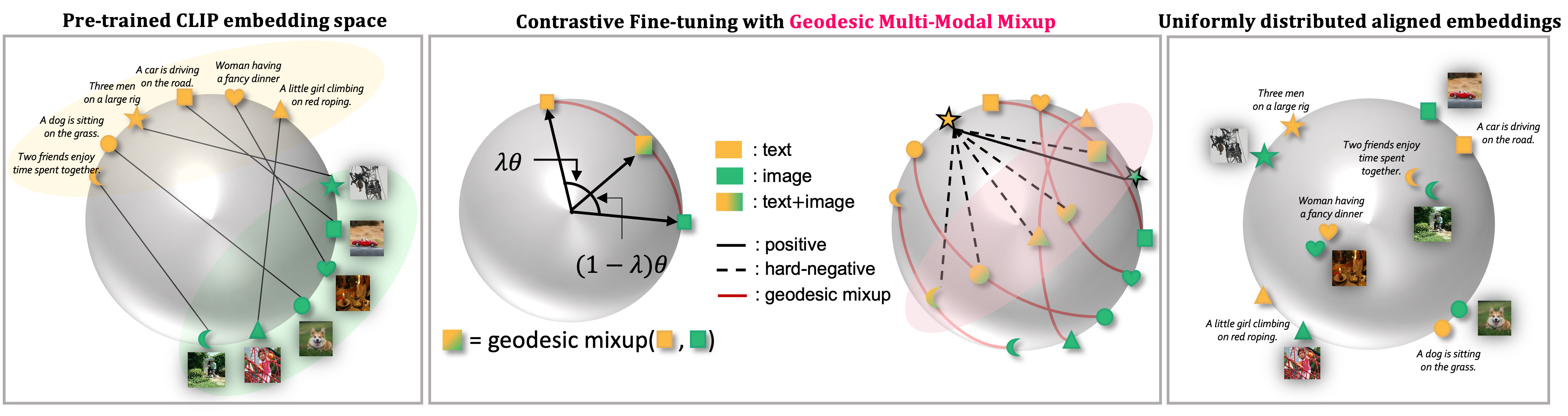
Figure 1: (Left) pre-trained CLIP has two separated clusters for image and text, with a large unexplored interspace. As a result, it has poor uniformity and alignment that might limit the embedding transferability. (Middle) For robust representation, our geodesic multi-modal Mixup ($m^{2}$-Mix) explores the unexploited interspace by mixing the heterogeneous embeddings on hypersphere. Generated samples by $m^{2}$-Mix are regarded as hard negatives for contrastive loss. (Right) As a result, fine-tuning with $m^{2}$-Mix induces robust representation with better transferability.

Liang et al. [27], concurrently (in terms of ArXiv preprints) took a similar observation, modality gap, which incurs a bunch of following works, and they also found that increasing temperature ($\tau$) in contrastive loss could somewhat reduce the embedding separation. However, varying the temperature requires manual engineering for each downstream task, and it incurs an inevitable trade-off between uniformity-alignment [26]. It raises an important question motivating this work: "How can we obtain a multi-modal representation dealing better with the uniformity-alignment for robust transfer?"

To answer this, we propose a fundamental learning method, geodesic multi-modal Mixup ($m^{2}$-Mix). As shown in Fig. 1, $m^{2}$-Mix blends the embeddings of different domains, e.g., image and text, and utilizes the mixtures as new entrees of contrastive loss. Our $m^{2}$-Mix contributes to robust representation learning in three perspectives. First, it generates hard negative samples which have high similarity with positives (incentivizing alignment), and they are known to be crucial for robust CL [28, 29, 26]. We provide a theoretical guarantee of the hardness of $m^{2}$-Mixed samples with empirical results. Second, $m^{2}$-Mix interpolates samples from heterogeneous domains to expand the effective embedding space (increasing uniformity) untapped by pre-trained CLIP, and this is further supported by the limiting behavior of $m^{2}$-Mix (see Prop. 4.2). Third, $m^{2}$-Mix produces virtual augmented samples in embedding space, so it endows a better perception on the out-of-distribution samples as well as in-distribution samples than standard CL.

Contributions: (1) We found that CLIP has a bipartite embedding space with poor uniformity-alignment, which may limit the embedding transferability for downstream tasks. (2) To address this, we propose a new fine-tuning method based on geodesic multi-modal Mixup, $m^{2}$-Mix. To our knowledge, this is the first work that adopts direct mixtures between heterogeneous embeddings. (3) We devised $m^{2}$-Mix as a geodesic Mixup to ensure the mixed embeddings are on a hypersphere, and this is beneficial for stable learning with $L_{2}$-normalized embeddings. (4) We validate our method by theoretical analyses and extensive experiments on retrieval, calibration, full-/few-shot classification (under distribution shift), embedding arithmetic, and image captioning.

2 Related Works

Contrastive Representation Learning

Contrastive Learning (CL) has been widely utilized for representation learning on various domains [15, 17, 30, 19, 31]. The goal of CL is to learn an embedding function that maps data into an embedding space so that semantically similar data have close embeddings. Most of CLs adopt $L_{2}$-normalized embedding [13, 14, 15, 19] for stable learning [32], and it makes the embeddings lie on a unit hypersphere. There are key properties to analyze the hyperspherical embeddings, so-called Uniformity and Alignment [25]. Better uniformity and alignment can be regarded as a higher embedding transferability, so it is related to performance on downstream tasks. However, uniformity-alignment analysis on multi-modal settings has not been sufficiently explored yet [33], and we found that CLIP has poor uniformity-alignment before and even after fine-tuning. Meanwhile, it is known that hard negatives for constructing contrastive pairs are necessary to increase the robustness of contrastive representation learning [34, 35, 26, 36]. To this end, we devise a new approach for multi-modal CL, which generates hard negatives and achieves better uniformity-alignment for robust and transferable representation.

Mixup

There have been numerous papers that claim Mixup [37] is helpful for robust representation learning and alleviates the overconfident problems and failure under distribution shift as well as the in-distribution accuracy [38, 39, 40]. Based on such success of Mixup, many works are adopting it as a component of learning frameworks (on vision [41, 42, 43, 44], language [45, 46, 47] and graph [48, 49]). Besides, CL with Mixup to help representation learning has also been studied. While traditional CL annotates as 1 for positive pairs and 0 for negative pairs, $i$-Mix [50] and Un-Mix [51] interpolate the images with ratio $\lambda$, and adopt contrastive loss with pseudo labels according to the mixing ratio $\lambda$. However, there are few works on Mixup for multi-modal learning [52, 53]. STEMM [52] mixes the speech and text features to align them in shared embedding space, but it cannot be widely used for multi-modal learning because of its architecture-specific design. Therefore, we propose $m^{2}$-Mix, that can be broadly adopted for robust multi-modal representation learning.

Multi-modal Learning

To build a universal intelligence system that simultaneously processes multi-modal data streams, some focus on developing unified frameworks for multi-modal perception [2, 3, 54, 4, 55], others aim at representation learning under multi-modal correspondence [19, 31, 56, 57]. This work focuses on CLIP [19], the representative multi-modal representation learner. Based on the generalizable embedding space, CLIP has been utilized on numerous tasks [58, 59, 60, 61], and there are many attempts to fine-tune it efficiently [62, 63, 64, 65]. Moreover, robust fine-tuning methods have also been actively studied for generalization on both in- and out-of-distribution data. Wortsman et al. [10] propose a weight-ensemble method that interpolates the pre-trained and fine-tuned weights, Kumar et al. [11] adopt a two-stage learning scheme that combines linear probing and fine-tuning, and Goyal et al. [66] adopt contrastive loss during fine-tuning on image classification. However, previous works have only focused on uni-modal settings and downstream tasks are restricted to the image classification. This paper provides robust fine-tuning methods for multi-modal settings.

3 Observations and Problem Define

For a given batch $D=\{x_{i},y_{i}\}_{i=1}^{M}$ of $M$ instances where $(x_{i},y_{i})$ denotes the $i$-th image-text pair, the goal of multi-modal learning is to learn the pair-wise relations between image and text. To do this, CLIP [19] learns image encoder $f(\cdot;\theta_{1})$ and text encoder $g(\cdot;\theta_{2})$, so that embedding pairs $\{I_{i},T_{i}\}_{i=1}^{M}=\{f(x_{i};\theta_{1}),g(y_{i};\theta_{2})\}_{i=1}^{M}$ get closer to each other. Note that $I_{i}$ and $T_{i}$ are $L_{2}$-normalized unit vectors in most vision-language models, and they lie on the hypersphere. For simplicity, we omit the learning parameters $\theta_{1}$ and $\theta_{2}$ from all the following equations. CLIP adopts InfoNCE-style [13] loss $C(\cdot,\cdot)$ to enforce the similarity between positive pairs $(x_{i},y_{i})$ and distance among all remain negative pairs $(x_{i},y_{j})$. This is formulated as below (Eq. 1):

$$\tiny\vspace{-0.7em}C(I,T)=\frac{1}{M}\sum_{i=1}^{M}-\log\frac{\exp({sim}(I_{i},T_{i})/\tau)}{\sum_{j=1}^{M}\exp{({sim}(I_{i},T_{j})/\tau)}}\;\;\;\;\;\;\mathcal{L}_{\text{CLIP}}=\frac{1}{2}(C(I,T)+C(T,I))\vspace{-0.7em}$$ (1)

Like many other CL approaches, CLIP uses a dot product as a similarity calculation ${sim}(\cdot,\cdot)$ between two vectors and governs $\tau$ as a learnable temperature that controls the scale of measured similarity. Now, we analyze the multi-modal embedding in terms of uniformity and alignment, well-known properties in uni-modal CL literature [25, 26] but unexplored in multi-modal settings. Alignment (Eq. 2) evaluates the difference between distances (or similarities) of positive pairs compared with the hardest negative pairs, while uniformity (Eq. 3) indicates how uniformly the data is distributed. The greater alignment and uniformity denote the more transferable representation [25, 26].

$$\vspace{-0.5em}\text{Alignment}:= \medmath{-\mathbb{E}_{(x_{i},y_{i})}\big{[}\|f(x_{i})-g(y_{i})\|_{2}^{2}-\min_{k\neq i}{\|f(x_{i})-g(y_{k})\|_{2}^{2}}\big{]}}$$ (2)

$$\text{Uniformity}:= \medmath{-\log{\mathbb{E}_{(x_{i},y_{j})}\big{[}\exp{(-2\|f(x_{i})-g(y_{j})\|_{2}^{2})}\big{]}}}\vspace{-0.5em}$$ (3)

Fig. 2 shows (Left) DOSNES [24] and (Middle) uniformity-alignment of CLIP’s embedding space on image-caption datasets after pre-trained (ZS), naively fine-tuned (FT), and fine-tuned with our method (Ours). Pre-trained CLIP embeddings are separated by two subspaces for image and text with wide interspace between them, and even after fine-tuning, this structure remains unchanged. As a result, CLIP and its fine-tuned embedding have poor uniformity and alignment, and this might limit the transferability and robustness of embeddings to downstream data. From this observation, we aim to learn a more transferable and robust multi-modal representation with multi-modal mixup. To validate the transferability and robustness of embeddings, besides evaluating uniformity-alignment, we perform diverse downstream tasks: retrieval, few-/zero-shot classification on in-distribution (ID), out-of-distribution (OOD), classification under modality missing, embedding arithmetic, and image captioning in Section 5. Here, our method produces well-aligned and uniformly distributed embeddings resulting in consistent downstream performance gains (Fig. 2 Right).

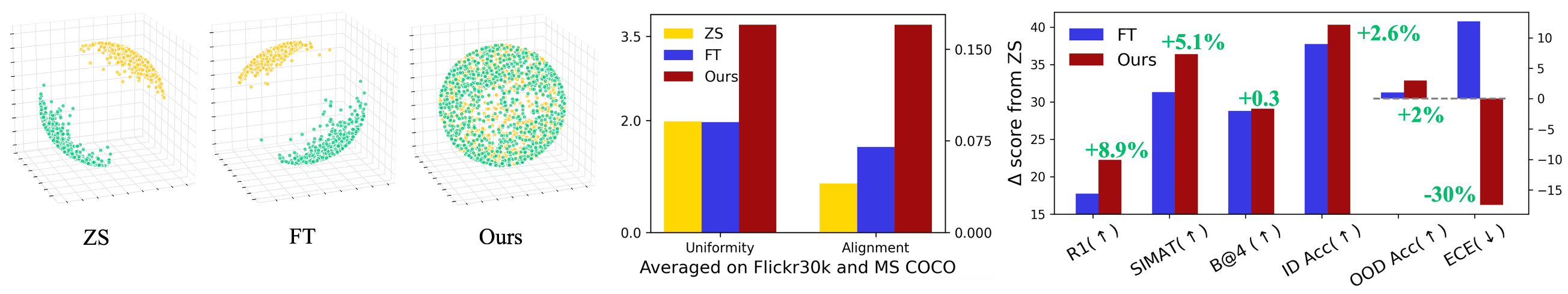
Figure 2: (Left) DOSNES [24] visualization of CLIP’s embedding space on Flickr 30k [67]. Greens and oranges denote the image and text embedding, respectively. Embeddings of pre-trained (ZS) and naively fine-tuned (FT) ones have two separate clusters with low uniformity and alignment (Middle), which may limit embedding transferability. Multi-modal mixup induces more aligned and uniformly distributed embeddings, (Right) which largely improves downstream performance, including retrieval (R1), embedding arithmetic (SIMAT), image captioning (BLUE@4), and classification (ID Acc. and OOD Acc.), and uncertainty calibration (ECE).

4 Methodology

4.1 Understanding Geodesic Multi-Modal Mixup

From our finding that CLIP embedding is not robust enough, we improve it by fine-tuning CLIP via contrastive loss with virtual hard negative samples. First, we generate hard negatives by mixing the image and text embeddings via multi-modal Mixup, $m^{2}$-Mix. Note that CLIP’s $L_{2}$-normalized embeddings lie on a hypersphere, and the mixed ones are also desirable to lie on that hypersphere. However, original Mixup [37, 41] does not guarantee that mixed data lie on the hypersphere. Therefore, we devise a new type of Mixup, geodesic Mixup (defined as Eq. 4). Geodesic Mixup interpolates two data points on geodesic path, so it ensures that mixed samples lie on the hypersphere.

$${\color[rgb]{0,0,0}m_{\lambda}(\vec{a},\vec{b})} =\vec{a}\frac{\text{sin}(\lambda\theta)}{\text{sin}(\theta)}+\vec{b}\frac{\text{sin}((1-\lambda)\theta)}{\text{sin}(\theta)},\;\;\;\text{where}\;\theta=\text{cos}^{-1}(\vec{a}\cdot\vec{b})\text{ and }\lambda\sim\text{Beta}(\alpha,\alpha)$$ (4)

Where $\lambda$ is handled by a hyperparameter $\alpha$ in Beta distribution. It is well-known that $L_{2}$-normalized embeddings are crucial for metric learning [68, 69] thus adopted by most of the modern contrastive learning methods [14, 15, 19]. Therefore, it is necessary that mixture samples lie on the unit sphere, which is guaranteed by our geodesic Mixup. Comparison between geodesic Mixup and standard Mixup following manual $L_{2}$-normalization in Tab. 6. Then, we utilize the generated hard negatives for contrastive loss by replacing the original negatives (See Eq. 5). Here, we only change the denominator term and retain the numerator that compares the similarity between the positive pairs.

$$C_{m^{2}}(I,T)=\frac{1}{M}\sum_{i=1}^{M}-\log\frac{\exp(I_{i}\cdot T_{i}/\tau)}{\exp(I_{i}\cdot T_{i}/\tau)+\sum_{j\neq i}\exp(I_{i}\cdot m_{\lambda}(I_{j},T_{j})/\tau)}$$ (5)

$$\mathcal{L}_{m^{2}\text{-Mix}}=\frac{1}{2}(C_{m^{2}}(I,T)+C_{m^{2}}(T,I))$$

Because CLIP has two-sided polarized embeddings, the similarity between the original image (or text) embedding and mixed embedding is larger than that between the original image and text embeddings. Therefore, $m^{2}$-Mix generates harder negative samples compared with original negatives. The existence of hard negative samples is known to be important in uni-modal CLs [25, 26], and we validate it under multi-modal CL settings in Section 5. Besides, we provide a theoretical result on hardness guarantee and limiting behavior of $\mathcal{L}_{m^{2}\text{-Mix}}$ in the following paragraph.

Theoretical Analysis

In Section 3, we observed that naive fine-tuning with standard contrastive loss could not reduce the embedding separation. We speculate this limitation is derived from (1) lack of hard negative samples and (2) vanished learnable $\tau$ (0.01) in $\mathcal{L}_{\text{CLIP}}$. As shown by Wang et al. [26], when $\tau$ approaches zero, the contrastive loss behaves like triplet loss with zero-margin. This means that if the similarity between positive samples is greater than that of the nearest negative, there are no incentives to further pull or push the embeddings of positive and negative samples. Moreover, due to CLIP’s bipartite embedding space, it might lack sufficient hard negative samples to incentivize the models to pursue more alignment and uniformity. Therefore, we argue that hard negatives are necessary for multi-modal CL when there is an embedding space modality gap [27].

Theorem 4.1 (Hardness of $m^{2}$-Mixed samples).

Let’s assume that two random variables $x_{1}$ and $x_{2}$ follow the $M_{d}(\mu_{1},\kappa)$ and $M_{d}(\mu_{2},\kappa)$, von Mises–Fisher distribution with mean direction $\mu_{1},\mu_{2}$ and concentration parameter $\kappa$ in $\mathbb{R}^{d}$, respectively. Let $\widetilde{x}=x_{1}+x_{2}$ and $d=2$. Then, $D_{KL}(p(x_{1})||p(\widetilde{x}))\leq D_{KL}(p(x_{1})||p(x_{2}))$ for sufficiently large $\kappa$.

Theorem 4.1 shows that KL-divergence between the pair of an original sample and a mixed sample is less (more confused with positive) than that of another original sample (proof in Supp. D). Meanwhile, because the converged $\tau$ of CLIP is significantly small (i.e., 0.01), it will be reasonable to consider an extreme case: when $\tau\to 0^{+}$. Based on Proposition 4.2, we argue that ones can explicitly enforce uniformity-alignment in multi-modal contrastive learning by equipping $m^{2}$-Mix with $\mathcal{L}_{\text{CLIP}}$.

Proposition 4.2 (Limiting behavior of $\mathcal{L}_{\text{CLIP}}$ with $\mathcal{L}_{m^{2}\text{-Mix}}$).

For sufficiently large $M$, as the temperature of contrastive loss $\tau\to 0^{+}$, the $\mathcal{L}_{\text{CLIP}}$ and $\mathcal{L}_{m^{2}\text{-Mix}}$ converges to the triplet loss with zero-margin (i.e., corresponding to negative Alignment) and negative Uniformity, respectively. That is: $\lim_{\tau\to 0^{+}}\mathcal{L}_{\text{CLIP}}+\mathcal{L}_{m^{2}\text{-Mix}}\simeq-(\text{Alignment}+\text{Uniformity})$

$m^{2}$-Mix brings two advantages on multi-modal CL with theoretical grounds. Firstly, by generating sufficiently hard negatives, it incentivizes the model to enforce alignment more strongly whether there exists a modality gap or not. Besides, the uniformity is also explicitly increased as $\mathcal{L}_{m^{2}\text{-Mix}}$ asymptotically converges to negative uniformity. Thus, $\mathcal{L}_{\text{CLIP}}$ with $m^{2}$-Mix induces well-aligned and uniformly distributed embeddings, so it makes the model robustly works on diverse tasks.

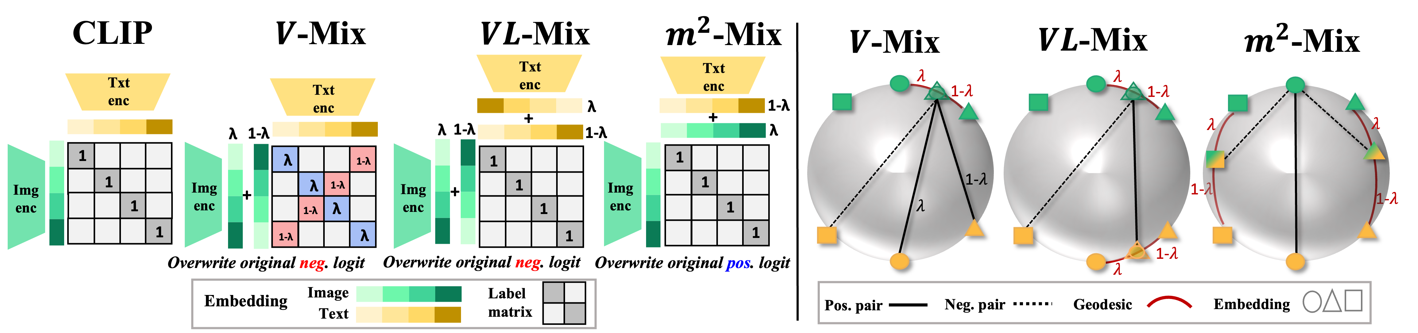
Figure 3: Comparison among contrastive losses. CLIP enforces the pair-wise similarity between matched image-text embedding pairs. $m^{2}$-Mix generates hard negative samples via mixing two heterogeneous embeddings. We additionally propose uni-modal Mixups, $V$-Mix (and $L$-Mix) and $VL$-Mix, that augment the homogenous embeddings in multi-modal contrastive loss.

4.2 Uni-Modal Mixup for CLIP

$m^{2}$-Mix generates hard negatives for CL to align and distribute embeddings uniformly. Meanwhile, Mixup is known to alleviate the overconfidence problem in uni-modal setups [38]. So, we further propose three uni-modal Mixups, Vision-Mix ($V$-Mix), Language-Mix ($L$-Mix), and Vision-Language Mix ($VL$-Mix) to enhance multi-modal CL. Fig. 3 shows the overall structures.

$uni$-Mix

$V$-Mix and $L$-Mix interpolate the image and text embedding, respectively. To be specific, $V$-Mix mixes the embeddings of images in batch and a flipped (reversed) batch with a ratio $\lambda$. Then, $m_{\lambda}(I_{i},I_{i^{\prime}})$ has information from $i$ and $i^{\prime}=M-i$ indexed samples with $\lambda$ and $1-\lambda$ fraction, respectively. Thus, pseudo label for $(m_{\lambda}(I_{i},I_{i^{\prime}}),T_{i})$ pair is $\lambda$ while, that for $(m_{\lambda}(I_{i},I_{i^{\prime}}),T_{i^{\prime}})$ is 1-$\lambda$.

$$C_{V}(I,T) =\frac{1}{M}\sum_{i=1}^{M}-\lambda\log\frac{\exp(m_{\lambda}(I_{i},I_{i^{\prime}})\cdot T_{i}/\tau)}{\sum_{j=1}^{M}\exp(I_{i}\cdot T_{j}/\tau)}-(1-\lambda)\log\frac{\exp(m_{\lambda}(I_{i},I_{i^{\prime}})\cdot T_{i^{\prime}}/\tau)}{\sum_{j=1}^{M}\exp(I_{i}\cdot T_{j}/\tau)}$$

$L$-Mix has the same formula with $V$-Mix, except that it is applied to text-side. The combination loss term of $V$- and $L$-Mix is defined as $\mathcal{L}_{uni\text{-Mix}}=\frac{1}{2}(C_{V}(I,T)+C_{V}(T,I))+\frac{1}{2}(C_{L}(I,T)+C_{L}(T,I))$

$VL$-Mix

For pair-wise similarity contrast, $V$-Mix and $L$-Mix only mix the image and text embedding, respectively. We additionally propose $VL$-Mix that mixes the image and text embedding simultaneously. Note that $m^{2}$-Mix mixes embeddings of image and text, while $VL$-Mix independently mixes them. Both $m_{\lambda}(I_{i},I_{i^{\prime}})$ and $m_{\lambda}(T_{i},T_{i^{\prime}})$ has $i$-th component and $i^{\prime}$-th component with fraction $\lambda$ and $1-\lambda$ respectively, so the pseudo label for $(m_{\lambda}(I_{i},I_{i^{\prime}})$, $m_{\lambda}(T_{i},T_{i^{\prime}}))$ is 1. Here, similarities between negative pairs are retain with that of original negatives likewise $uni$-Mix.

$$C_{VL}(I,T)=\frac{1}{M}\sum_{i=1}^{M}-\log\frac{\exp(m_{\lambda}(I_{i},I_{i^{\prime}})\cdot m_{\lambda}(T_{i},T_{i^{\prime}})/\tau)}{\sum_{j=1}^{M}\exp(I_{i}\cdot T_{j}/\tau)}\;\;\mathcal{L}_{VL\text{-Mix}}=\frac{1}{2}(C_{VL}(I,T)+C_{VL}(T,I))$$

$m^{3}$-Mix

We name the combination of $m^{2}$-Mix with uni-Mix and $VL$-mix as $m^{3}$-Mix, multiple multi-modal Mixup. Complete objective function is denoted as (weights for each term are omitted):

$$\mathcal{L}_{m^{3}\text{-Mix}}=\mathcal{L}_{CLIP}+\mathcal{L}_{m^{2}\text{-Mix}}+\mathcal{L}_{uni\text{-Mix}}+\mathcal{L}_{VL\text{-Mix}}$$

5 Results

Settings

Unless otherwise stated, we adopt CLIP ViT-B/32 as our backbone model. We consider the following methods as our baselines in retrieval and embedding arithmetic tasks: zero-shot inference (ZS) of CLIP, embedding shift (ES) [27], naive fine-tuning (FT), and its increased $\tau$ variants, recent Mixup-augmented uni-modal CL methods $i$-Mix [50] and Un-Mix [51]. We put task-specific setups on each section and Sec. A of Supplementary Material (SM). Further details, hyperparameters selection, pseudo code, and additional results are put in Sec. A, B, and C of SM, respectively.

5.1 Generated Samples by $m^{2}$-Mix

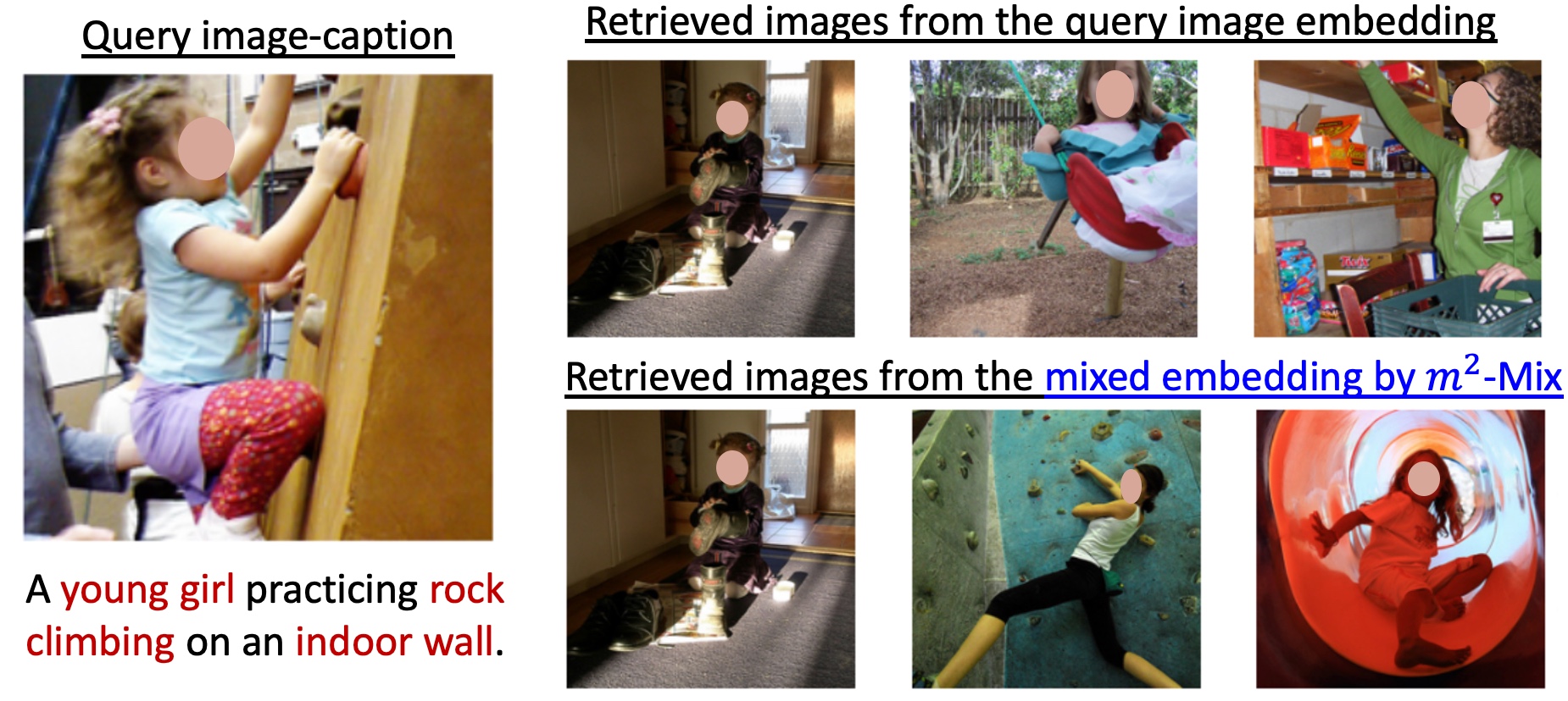
(a) Retrieved images

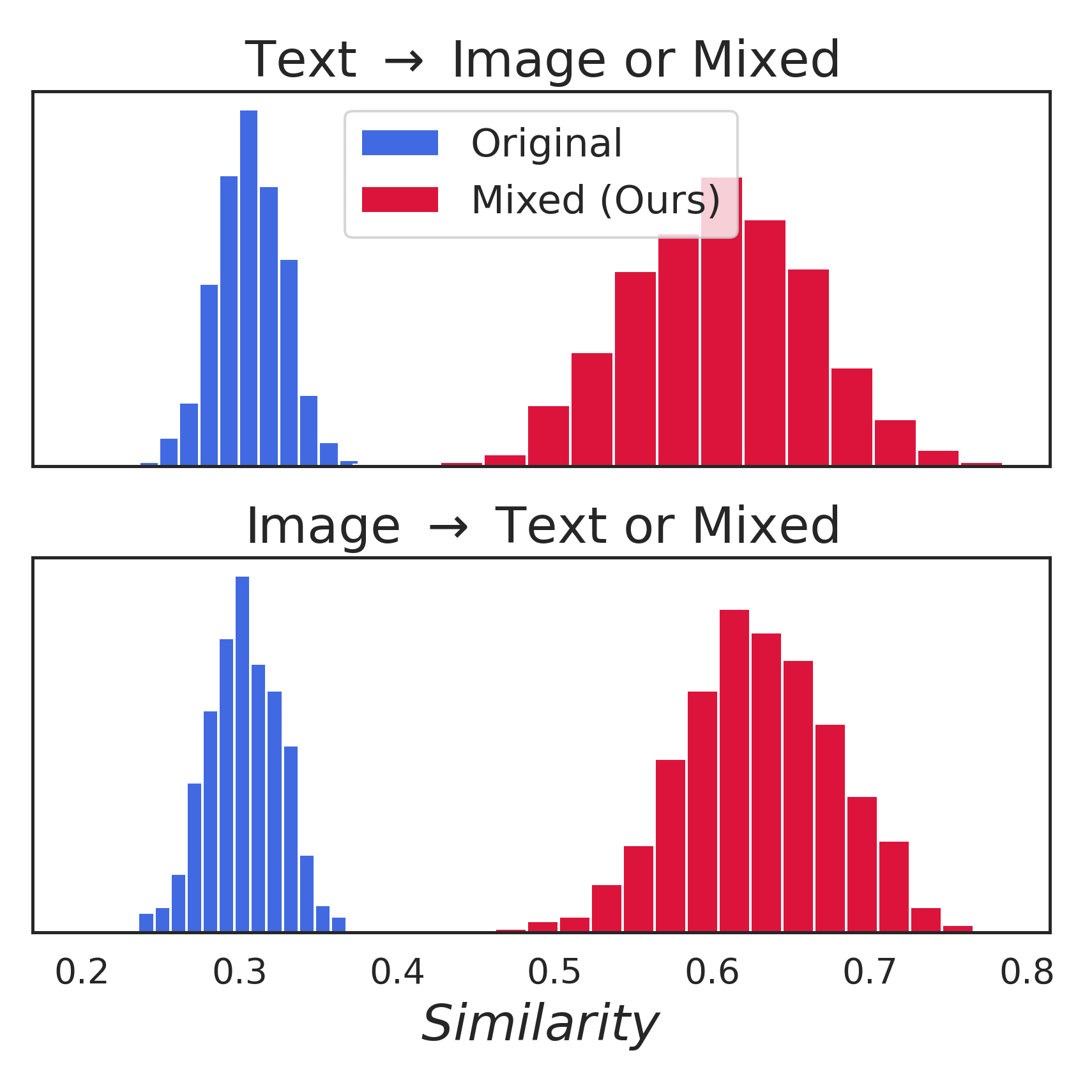
(b) Initial epoch

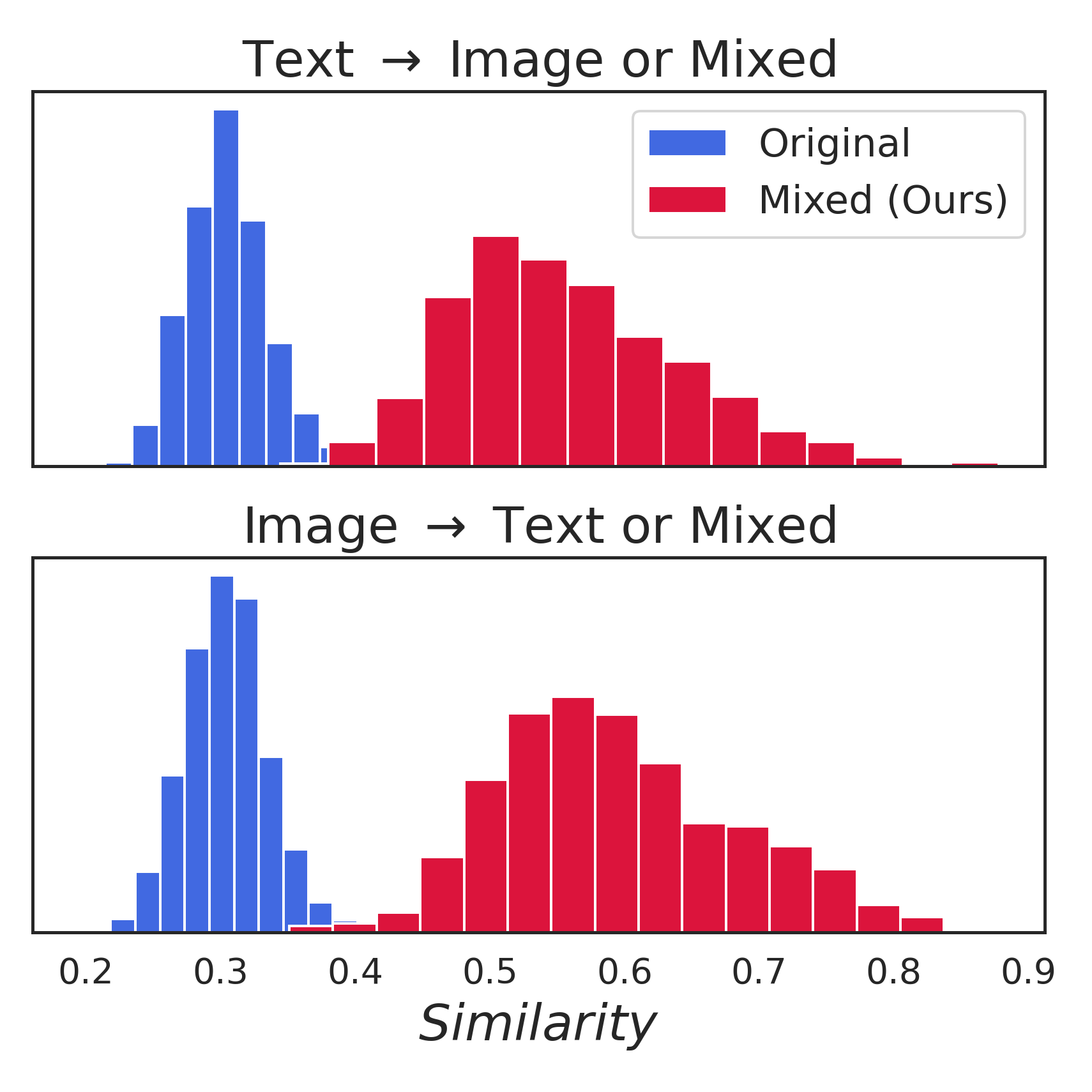
(c) Last epoch

Figure 4: On Flickr30k, (a) top-3 retrieved images by image embedding (Top) and $m^{2}$-Mixed (Bottom) from a source instance (Left). $m^{2}$-Mix generates an embedding that contains features from both modalities (young girl, climbing, and indoor wall), partly lacking in the image embedding. (b) and (c) denote cosine similarities between given test instances and its top-1 nearest negative embedding during training epochs. $m^{2}$-Mix makes negatives that are highly similar to given instances.

To understand the properties of generated embedding by $m^{2}$-Mix, we explore the mixed embedding from $m^{2}$-Mix. Due to the non-trivial visualization of the embedding itself, we retrieve images that have the most similar embedding with a mixed one. In Fig. 4 (a), the embedding generated by $m^{2}$-Mix has both features from image and text that lack in original image embedding, e.g., the second and third images from $m^{2}$-Mix have rock climbing and indoor wall represented in the text. Besides, similarity histograms in Fig. 4 (b) and (c), show that $m^{2}$-Mix consistently produces harder negatives than the original non-mixed counterparts from the initial to last training epochs.

5.2 Cross-Modal Retrieval with CLIP

First, we validate our method on image-text retrieval, a representative vision-language task, on Flickr30k [67] and MS COCO [70]. All methods are trained over 9 epochs with Adam optimizer (details in SM). Tab. 1 denotes top-1/-5 recall of retrieval. Our $m^{3}$-Mix increases overall performance, while the standard fine-tuning approaches and Mixup-baselines [50, 51] have limited performance gain. Corresponding to previous works [26, 27], we also found that properly increasing temperature ($\tau$) in contrastive loss is quite beneficial at improving performance for both FT and $m^{3}$-Mix.

Table 1: Image to text (i$\rightarrow$t) and text to image retrieval (t$\rightarrow$i) retrieval results (top-1/-5 Recall;R1, R5). ZS and FT denote pre-trained and fine-tuned CLIP, respectively.

	Flickr30k				MS COCO
	i$\rightarrow$t		t$\rightarrow$i		i$\rightarrow$t		t$\rightarrow$i
	R1	R5	R1	R5	R1	R5	R1	R5
ZS	71.1	90.4	68.5	88.9	31.9	56.9	28.5	53.1
ES [27]	71.8	90.0	68.5	88.9	31.9	56.9	28.7	53.0
FT	81.2	95.4	80.7	95.8	36.7	63.6	36.9	63.9
FT ($\tau=0.05$)	82.4	95.1	82.1	95.7	40.2	68.2	41.6	69.9
FT ($\tau=0.10$)	75.7	93.9	78.0	92.9	34.2	62.7	36.7	64.2
$i$-Mix [50]	72.3	91.7	69.0	91.1	34.0	63.0	34.6	62.2
Un-Mix [51]	78.5	95.4	74.1	91.8	38.8	66.2	33.4	61.0
$m^{3}$-Mix	82.3	95.9	82.7	96.0	41.0	68.3	39.9	67.9
$m^{3}$-Mix ($\tau=0.05$)	82.7	95.7	82.8	95.5	40.4	67.9	42.0	68.8

Table 2: Retrieval with disjoint uni-modal models. ZS is a naive combination of two models without joint-tuning.

	Flickr30k
	i $\rightarrow$ t		t $\rightarrow$ i
	R1	R5	R1	R5
ZS	0.1	0.4	0.1	0.2
ES [27]	0.1	0.5	0.2	0.2
FT	28.7	61.7	26.7	59.4
FT ($\tau=0.05$)	31.5	64.2	29.2	61.4
FT ($\tau=0.10$)	30.0	62.7	30.1	60.6
$i$-Mix [50]	27.6	60.3	27.1	60.7
Un-Mix [51]	31.5	64.3	29.2	61.2
$m^{3}$-Mix	31.9	62.6	30.3	61.0
$m^{3}$-Mix ($\tau=0.05$)	32.5	64.7	30.4	63.4

Table 3: Calibration on Flickr30k.

Metric	Task	ZS	FT	$m^{3}$-Mix
ECE ($\downarrow$)	i $\rightarrow$ t	1.90	2.26	1.54
	t $\rightarrow$ i	1.88	2.00	1.58

Besides, we observed the improved uniformity and alignment by $m^{3}$-Mix (Fig. 2) not only enhances the Recall of retrievals but also contributes to the calibration [71]. The left side of Fig. 5 denotes the reliability diagrams with calibration errors of the text-to-image retrieval R1 score on Flickr30K. While the naively fine-tuned CLIP has poor calibration, fine-tuning with $m^{3}$-Mix alleviates the overconfidence issue somewhat and results in a better calibration. This is further confirmed by Tab. 3, in which our $m^{3}$-Mix significantly improves the Expected Calibration Error (ECE) of CLIP. Meanwhile, it is known that the ECE value can be improved by adjusting the temperature $\tau$, i.e., temperature scaling [71]. Therefore, we provide the sensitive analysis on varying $\tau$. In Fig. 5 right side, our method shows relatively robust ECE under varying $\tau$, implying that our multi-modal Mixup-based CL induces the well-calibrated multi-modal model, which is crucial for reliable AI applications.

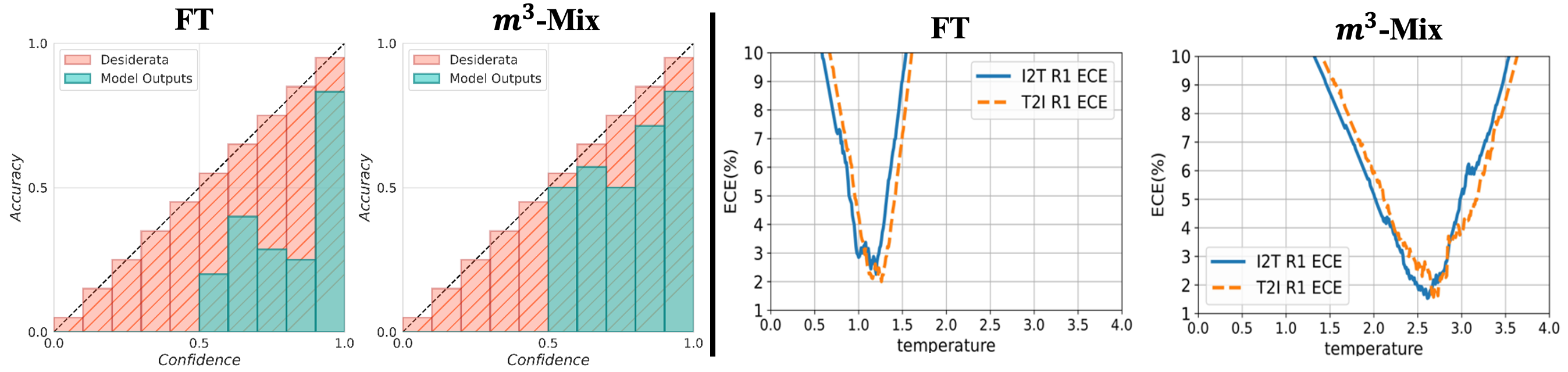
Figure 5: Reliability diagram (left) and ECE under varying temperature $\tau$ (right) on Flickr30K image-to-text retrieval. Our method shows (1) a better reliability diagram (close to $y=x$), (2) achieves a lower minimum ECE value, and (3) more stable across varying $\tau$ than naive fine-tuning. Thus, representation learning by $m^{3}$-Mix robustly induces a well-calibrated multi-modal model.

5.3 Cross-Modal Retrieval with Uni-Modal Pre-Trained Models

Sometimes, the high-quality annotations for multi-modal datasets are expensive, and there are cases when plenty of paired multi-modal data is unavailable. Then, it is crucial to exploit the uni-modal pre-trained models for learning multi-modal embedding space [72]. To this end, we validate our $m^{3}$-Mix on the fine-tuning of disjointly pre-trained uni-modal models. Specifically, we jointly fine-tune the pre-trained BERT [73] and ResNet-50 [74] with a contrastive loss on Flickr30k (in Table 5.2). Among candidates, $m^{3}$-Mix with higher $\tau$ consistently achieves the highest performance so that it can be adopted as an effective joint tuning method for independently pre-trained uni-modal models.

5.4 Few-Shot Adaptation and Robustness on Distribution Shift

Table 4: Few-shot adaptation under general setting.

Method	Dataset
	Pets	SVHN	CLEVR	Avg.
ZS	87.49	13.63	20.70	40.61
FT	89.37	45.00	53.49	62.62
FT w/ $V$-Mix	89.45	44.61	53.93	62.66
FT w/ $L$-Mix	89.43	48.42	53.91	63.92
FT w/ $VL$-Mix	89.56	45.22	53.75	62.84
FT w/ $m^{2}$-Mix	90.05	46.24	53.60	63.29
$m^{3}$-Mix	90.16	54.84	53.85	66.28
$m^{3}$-Mix ($\tau=0.05$)	90.49	60.90	53.95	68.45
WiSE-FT [10]	91.80	35.04	41.93	56.25
WiSE-FT w/ $m^{3}$-Mix	92.51	58.55	47.11	66.06
LP-FT [11]	89.92	44.91	53.62	62.82
LP-FT w/ $m^{3}$-Mix	91.03	64.24	55.20	70.16
MaPLe [64]	90.87	47.62	43.05	60.51
MaPLe w/ $m^{3}$-Mix	91.14	52.72	45.20	63.02

Table 5: Few-shot (ImageNet; IN) and zero-shot evaluation under distribution shift (-V2, -A, -R, -S).

Method	Dataset
	IN	IN-V2	IN-A	IN-R	IN-S	Avg.
ZS	62.06	54.80	29.63	66.02	40.82	50.67
FT	65.44	55.35	20.07	58.16	34.50	46.70
FT w/ $V$-Mix	66.00	56.19	20.85	60.50	34.97	47.70
FT w/ $L$-Mix	65.96	55.95	20.57	60.54	35.25	47.65
FT w/ $VL$-Mix	66.24	56.70	21.36	61.07	35.11	48.10
FT w/ $m^{2}$-Mix	67.04	57.39	20.05	59.28	35.31	47.81
$m^{3}$-Mix	67.08	57.55	20.80	60.96	35.86	48.45
$m^{3}$-Mix ($\tau=0.05$)	68.40	58.51	22.17	62.28	37.62	49.80
WiSE-FT [10]	69.00	59.66	28.01	64.84	41.05	52.51
WiSE-FT w/ $m^{3}$-Mix	69.65	60.71	29.16	66.75	42.19	53.69
LP-FT [11]	68.22	58.40	25.57	63.36	38.04	50.72
LP-FT w/ $m^{3}$-Mix	68.62	59.17	25.85	65.14	38.78	51.51
MaPLe [64]	65.59	58.44	32.49	68.13	42.53	53.44
MaPLe w/ $m^{3}$-Mix	65.76	58.16	32.52	68.20	42.67	53.46

Next, we evaluate our methods on few-shot image classification under general (in Tab. 5.4) and distribution shift settings (in Tab. 5.4 and 6). We consider OxfordPets [75], SVHN [76], and CLEVR [77] for the general setting and ImageNet-1k, ImageNetV2 [78], ImageNet-A [79], ImageNet-R [80], and ImageNet-Sketch [81] for distribution shift setting. Unlike MS COCO and Flickr30K, These datasets provide class name labels only and do not have captions corresponding to each image. To make CL methods amendable for this setting, we adopt a common prompt ’a photo of classname’ that wraps the class name with a short context and use this as captions of images. Following [82, 64], we perform the tasks under a few-shot evaluation protocol: 16-shot training samples per class and inference on the entire test set.

Table 6: Ablation study on Mixup.

Temperature ($\tau$)	$m^{3}$-Mix type
	linear	geodesic
0.01	48.36	48.45
0.05	48.48	49.80
0.10	45.20	46.41

As baselines, we first consider zero-shot CLIP (ZS) and construct the contrastive loss adoption of vanilla fine-tuning (FT). Then, we showcase our methods with exhaustive ablation ($V$-, $L$-, $VL$-, and $m^{2}$-Mix) as well as our complete objective $m^{3}$-Mix with its high-temperature variant. To further compare our approach with state-of-the-art (SOTA) fine-tuning methods, we consider MaPLe [64] that optimizes the continuous prompts inside the text and image encoders of CLIP, and the contrastive loss extended version of uni-modal fine-tune methods: LP-FT [11] and WiSE-FT [10].

In both general and distribution shift settings, $m^{2}$-Mix and uni-modal Mixups ($V$-, $L$-, $VL$-) contribute to boost the few-/zero-shot classification performance. After integrating them, $m^{3}$-Mix and its high-temperature variant give significant performance improvement, implying $m^{3}$-Mix is an effective fine-tuning method that covers challenge generalization setup. Moreover, when $m^{3}$-Mix combined with SOTA fine-tuning methods [10, 11, 64], it consistently brings performance. Therefore, $m^{3}$-Mix is a flexible plug-in method that can be collaborated with many algorithms. Besides, in Tab. 6 (mean Acc. of ImageNet variants), we show that geodesic Mixup achieves superior results than linear Mixup with manual $L_{2}$-normalization. Thus, based on its analytic property, geodesic Mixup is more suitable than linear Mixup under frameworks that learn representation on a hypersphere, as in modern CLs.

5.5 Robustness on Modality Missing

In this section, we study whether $m^{2}$-Mix can help the multi-modal representation learning for video recognition (CMU-MOSEI [83]) under modality missing. Recently, Geometric Multi-modal Contrastive Learning (GMC) [84] achieved competitive results on CMU-MOSEI.

However, GMC only considers the uni-to-joint modal relationship [84], while our $m^{2}$-Mix explicitly generates the mixture of bi-modal semantics so that it can additionally consider the bi-to-joint modal relation. From this, we hypothesize that $m^{2}$-Mix can further improve the robustness and informativeness of the representation. For evaluation, we add the $m^{2}$-Mix on top of GMC.

Figure 6: t-SNE [85] on CMU-MOSEI with partial information. Each color denotes embeddings of partial and joint modality.

Different from the CLIP fine-tuning cases, we use the multi-modal mixed representation as both positive and negative pairs with the target joint representation because our goal in this task is to align the embedding between the joint and other modalities. As shown in Tab. 7, $m^{2}$-Mix coherently improves the performance of GMC in terms of accuracy, alignment, and uniformity. While GMC strongly aligns the embedding of partial and joint modality, the alignment is further enhanced by the aid of $m^{2}$-Mix (also confirmed in Fig. 6), which results in superior performance when only partial information is given in test-time (modality missing). These results justify the use of $m^{2}$-Mix for robust learning under modality-incomplete scenarios.

Table 7: Accuracy (acc.)($\uparrow$), alignment (align.)($\uparrow$), and uniformity (unif.)($\uparrow$) of multi-modal learning methods on CMU-MOSEI under complete and partial modalities. Averaged performance of five runs.

Test-time Observed Modalities Full (T+V+A) T V A T+V T+A V+A acc. unif. acc. align. unif. acc. align. unif. acc. align. unif. acc. align. unif. acc. align. unif. acc. align. unif. MulT [86] 80.5 0.99 60.0 - 1.03 53.9 - 2.07 52.7 - 0.62 57.8 - 1.27 58.8 - 0.77 54.6 - 1.36 GMC [84] 80.1 3.06 78.5 0.20 3.03 64.7 0.17 3.01 66.0 0.09 3.03 77.0 0.07 2.94 77.4 0.08 3.00 67.3 0.05 2.98 GMC+$m^{2}$-Mix 80.5 3.18 78.9 0.23 3.17 64.2 0.19 3.15 66.2 0.12 3.15 77.8 0.08 3.08 77.9 0.09 3.08 67.4 0.06 3.10

5.6 Multi-Modal Embedding Arithmetic

We expect that well-learned multi-modal embedding represents the structural relationship between instances like word vectors [87]. For validation, we evaluate the learned embeddings on SIMAT [88]. SIMAT evaluates text-driven image representation by retrieving a new image with the highest similarity to the latent vector $x$, which is transformed by text delta vectors when we change the word in an original text, i.e., formulated as: $x=I_{original}+\lambda\cdot(T_{new}-T_{original})$. Here, $I$ and $T$ are image and text embedding vectors, and $\lambda$ is a hyper-parameter about the strength of transformation. Table 8 presents the quantitative scores across methods after fine-tuning on Flickr30k and MS COCO, and evaluated on SIMAT. Learned representation from $m^{3}$-Mix shows stable scores on both a multi-modal model and jointly fine-tuned uni-modal models, which is further confirmed by qualitative experiments (Fig. 7). These support that $m^{3}$-Mix can be adopted as a delicate fine-tuner when embedding geometric structure and arithmetic property should be considered, e.g., controllable generation [89].

Table 8: $m^{3}$-Mix shows the stable SIMAT Score ($\uparrow$) on CLIP and joint fine-tuning of uni-modal pre-trained models.

	CLIP	CLIP	BERT + RN50
	(MS COCO)	(Flickr30k)	(Flickr30k)
ZS	34.5	34.4	6.1
ES [27]	34.6	34.5	6.2
FT	42.3	40.8	15.4
$i$-Mix [50]	37.3	40.0	12.9
Un-Mix [51]	42.9	38.5	15.8
$m^{3}$-Mix	44.4	38.9	19.0

Figure 7: Embeddings of $m^{3}$-Mix on SIMAT source-target texts (reds) and images (source and top-1 retrieved). Black texts correspond to top-3 retrieved images from a source image-caption.

5.7 Multi-Modal Mixup on a State-of-the-Art Vision-Language Model

In this section, we investigate whether our multi-modal Mixup can also be beneficial for improving other recent large-scale vision-language models beyond CLIP. For this, we adopt Contrastive Captioner (CoCa) [90] ViT-L/14 configuration that pre-trained on LAION-2B [5] from OpenCLIP library as our target backbone model. We consider three learning objectives for CoCa fine-tuning: (1) autoregressive captioning loss (Cap), (2) contrastive loss and captioning loss (CL $+$ Cap), and (3) contrastive loss, $\mathcal{L}_{m^{2}\text{-Mix}}$, and captioning loss (CL w/ $\mathcal{L}_{m^{2}\text{-Mix}}+$ Cap). For all three methods, we train the model on MS COCO over one epoch with OpenCLIP-provided hyperparameter configuration. After that, we evaluate each model for image captioning (Tab. 9) on MS COCO and zero-shot and fine-tuned cross-modal retrieval (Tab. 10) on Flickr30K and MS COCO.

Table 9: Image captioning results on MS COCO with CoCa ViT-L/14 model. We fine-tune the CoCa on MS COCO for 1 epoch with three different learning objectives and evaluate them in terms of five conventional metrics. $m^{2}$-Mix achieves performance gain on all the five metrics.

Method	Metrics
	BLEU@4	METEOR	ROUGE-L	CIDEr	SPICE
ZS	7.2	12.4	26.3	35.2	9.3
Cap	36.0	29.4	57.3	125.1	23.1
CL + Cap	35.7	29.3	57.1	124.9	23.0
CL w/ $\mathcal{L}_{m^{2}\text{-Mix}}$ + Cap	36.3	29.5	57.5	125.6	23.2

In Tab. 9, while a combination of vanilla contrastive loss with captioning loss underperforms the captioning-loss-only training, $m^{2}$-Mix-assisted contrastive learning further increases the performance on image captioning in terms of five conventional metrics. Besides, Tab. 10 shows that $m^{2}$-Mix generally improves the retrieval recalls of CoCa on zero-shot and fine-tuned settings. This implies that representation learning with our multi-modal Mixup is beneficial to generative tasks as well as discriminative tasks. The consistent improvement shown in the image captioning task is accorded with observations from other recent works [52, 53] that reveal the effectiveness of cross-modal Mixup on generative tasks by increasing cross-modal alignment.

Table 10: Cross-modal retrieval top-1/5 recalls on MS COCO (fine-tuned) and Flickr30k (zero-shot transfer). $m^{2}$-Mix generally enhances image-text retrieval of a SOTA vision-language model, CoCa.

Method	(Zero-shot) Flickr30k
	i $\rightarrow$ t (R1)	i $\rightarrow$ t (R5)	t $\rightarrow$ i (R1)	t $\rightarrow$ i (R5)
Cap	90.4	98.5	78.5	94.4
CL + Cap	92.4	99.1	79.2	94.9
CL w/ $\mathcal{L}_{m^{2}\text{-Mix}}$ + Cap	92.8	99.0	79.5	95.1
Method	(Fine-tuned) MS COCO
	i $\rightarrow$ t (R1)	i $\rightarrow$ t (R5)	t $\rightarrow$ i (R1)	t $\rightarrow$ i (R5)
Cap	68.5	87.9	53.2	77.8
CL + Cap	73.9	91.2	56.3	80.4
CL w/ $\mathcal{L}_{m^{2}\text{-Mix}}$ + Cap	73.9	91.0	56.5	80.6

6 Conclusion

This paper analyzes the representation learned by a multi-modal contrastive learner. We found that CLIP has separated text-versus-image embedding space with poor uniformity-alignment. These polarized embeddings with huge unexploited space may limit the transferability and robustness of representation on downstream tasks. From our findings, we propose Geodesic Multi-Modal Mixup that generates hard negatives for robust contrastive learning by mixing two heterogeneous embeddings. Theoretically, we validate that our method produces hardness-guaranteed samples and has desirable asymptotic behavior to induce better generalizable representation. Empirically, the proposed method effectively improves performances on diverse tasks and perspectives: retrieval, calibration, few-shot classification under distribution shift, embedding arithmetic, and image captioning.

Though the increased uniformity and alignment of multi-modal representation largely empowers the model to adapt robustly to a diverse range of tasks, we found that reckless uplift of them is harmful in some cases of retrieval (modest increment of uniformity-alignment was better than huge increment of them). Thus, more research on the reliable evaluation of multi-modal representation should be pursued in the era of foundation models.

Acknowledgement

This work was supported by the National Research Foundation of Korea (NRF) grant funded by the Korea government (MSIT) (No.2021R1F1A1060117 and No.2022R1A4A3033874), and also supported by a grant (22183MFDS431) from Ministry of Food and Drug Safety in 2023.

Appendix A Experiment Setup

We first elaborate on the setups for all the experiments, including retrieval and embedding arithmetic, uni-modal classification, multi-modal classification, and Contrastive Captioner (CoCa) image captioning and retrieval, in each separate section.

A.1 Cross-modal Retrieval and SIMAT

Dataset

Here, we hold the Flickr30k and MS COCO, two representative vision-language benchmark datasets. Flickr30k contains 30K image-text pairs as a train split, 1k for validation and test splits. For MS COCO, we adopt the 2017 version of it from the COCO Database. MS COCO contains 118k image-text pairs for train split and 5k for both validation and test splits. When there are multiple captions for one image, we always select the first caption to construct an image-text pair. To validate the multi-modal embedding arithmetic, we use the SIMAT dataset [88]. SIMAT is a benchmark created for evaluating the text-driven image transformation performance of multi-modal embedding. It contains 6k images, 18k transformation queries that have pairs of (source word, target word, source image, target image), and 645 captions constructed with subject-relation-object triplets that have at least two corresponding images. The goal of SIMAT task is to retrieve an image, which is well-modified by a specific text transform to match with the ground truth transform target images.

Model Description

For retrieval and embedding arithmetic tasks, we adopt CLIP ViT-B/32 checkpoint of OpenAI official lease as our backbone model. For cross-modal retrieval with disjointly pre-trained uni-modal models, we utilize ResNet-50 [74] with a pre-trained checkpoint of torchvision as an image encoder and BERT-base-uncased from HuggingFace as a text encoder. To match the dimensions of these two uni-modal models, we add a projection head on top of each encoder, respectively.

Baseline Methods

First, we consider the zero-shot inference of CLIP (ZS) [19] as a strong baseline (in the case of retrieval with uni-modal pre-trained models, we just project the image and text embeddings to shared vector space with randomly initialized matrix, and perform similarity-based inference as ZS.), and embedding shift (ES) [27] which computes a delta vector (difference between mean vectors of image and text embeddings) and then manually modifies the modality gap along with delta vector direction without explicit training. Then, a vanilla fine-tuning (FT) with standard contrastive loss (Eq. 1 of main paper) and its higher-temperature variants ($\tau=\{0.05,0.01\}$) are considered. Additionally, we take account of two uni-modal mixup-based contrastive learning methods $i$-Mix [50] and Un-Mix [51] those mix images in the input space. While the original implementation of $i$-Mix takes a randomly sampled image as a mixture component, we take a flipped batch sample as a mixture component for computational efficiency like as Un-Mix. So the only difference between $i$-Mix and Un-Mix is whether we construct the final objective as a sum of normal and mixed sample contrastive loss [51] or sorely mixed sample contrastive loss ([50]).

Metric

As a standard metric for retrieval tasks, we report top-1 recall (R1) and top-5 recall (R5) on both image-to-text and text-to-image directions. For SIMAT task, following the original paper [88], we performed the OSCAR-based evaluation and reported the SIMAT score in the original paper. It measures the similarity between the transformed image and text captions via OSCAR framework [91].

Implementation Detail

We fine-tune CLIP with eval() mode stable training and under FP16 precision for computational efficiency. On both Flickr30k and MS COCO, we train each method over 9 epochs with batch size 128 via Adam optimizer ($\beta_{1}=0.9$, $\beta_{2}=0.98$, and $\epsilon=1e-6$). As shared hyperparameters, we search for the best initial learning rate from {1e-6, 3e-6, 5e-6, 7e-6, 1e-5} and weight decay from {1e-2, 2e-2, 5e-2, 1e-1, 2e-1} for all training methods (Initial learning rate is decayed in each epoch by the exponential scheduler with decaying parameter 0.9). To construct our complete objective $m^{3}\text{-Mix}$, we weighing the $L_{\text{CLIP}}$ and $L_{m^{2}\text{-Mix}}$ and uni-modal geodesic Mixup variants ($L_{V/L/VL\text{-Mix}}$). Specifically, we pivot the weight of $L_{\text{CLIP}}$ as 1.0 and sweep the weighting coefficient of other loss components for each dataset generally from {0.0, 0.01, 0.1, 0.2, 0.3, 0.5}. The parameter $\alpha$ of Beta distribution $Beta(\alpha,\alpha)$ that determines the mixture ratio is set to 0.5 for the multi-modal Mixup and 2.0 for uni-modal Mixups. For embedding shift (ES) [27], we sweep $\lambda$ from -0.1 to 0.1 by 0.01 and report the best results among them. While the search range of ES from official implementation is from -2.5 to 2.5 by 0.125, we observe the finer search range gives better results.

A.2 Uni-modal Classification

Dataset

We consider three common transfer learning benchmark datasets, OxfordPets [75], SVHN [76], and CLEVR [77], to validate the general few-shot adaptation capability. For evaluation of robustness on distribution shift, we consider the ImageNet-1k as a source dataset (models are adapted to) and ImageNetV2 [78], ImageNet-A [79], ImageNet-R [80], and ImageNet-Sketch [81] as target evaluation datasets those are considered as different kinds of natural distribution shift from ImageNet.

Model Description

For uni-modal few/zero-shot classifications, we also adopt CLIP ViT-B/32 as the default backbone for ours and baseline fine-tuning methods in our manuscript and also evaluate CLIP ViT-B/16 and CyCLIP ResNet50 in Section C of this Supplementary Material.

Baseline Methods

As standard baselines, we first consider zero-shot CLIP (ZS) and vanilla fine-tuning (FT) with contrastive loss. Then, we perform exhaustive ablation ($V$-, $L$-, $VL$-, and $m^{2}$-Mix) as well as our complete objective $m^{3}$-Mix with its high-temperature variant. To further compare our approach with state-of-the-art fine-tuning methods, we consider MaPLe [64] that optimizes the continuous prompts inside the text and image encoders of CLIP, and the contrastive loss extended version of uni-modal fine-tune methods: LP-FT [11] which trains classification head and full modal separately in a two-stage manner, and WiSE-FT [10] which performs parameter-space ensemble between the pre-trained checkpoint and fine-tuned checkpoint. Additionally, we consider the ES and our $m^{3}\text{-Mix}$ as the plug-in methods to improve the above three state-of-the-art fine-tuning methods that are denoted as method names w/ ES or $m^{3}\text{-Mix}$ in Tab. 4 and 5 of the main paper.

Metric

For both the few-shot adaptation and distribution shift setting, we report top-1 accuracy as the In-Distribution Accuracy (ID Acc.) and Out-Of-Distribution Accuracy (OOD Acc.), respectively.

Implementation Detail

In this paper, we propose new contrastive losses $m^{2}\text{-Mix}$ and $m^{3}\text{-Mix}$ which consume the image-text paired instances. However, the above datasets provide class name labels only and do not have captions corresponding to each image. To make CL methods amendable for this setting, we adopt a common prompt ’a photo of classname’ that wraps the class name with a short context and use this as captions of images. Different from image-caption-based contrastive learning on Flickr30k and MS COCO, a batch of ImageNet-1K contains multiple samples that are assigned to the same class. We construct the label map for contrastive loss by regarding all of the samples from a class as positives. Following [82, 64], we perform the tasks under the same few-shot evaluation protocol: 16-shot training samples per class and inference on the entire test set. To construct the contrastive loss, we first compute the pivot classifier embedding by forwarding all possible class category names to the text encoder. Then, we calculate the pairwise similarity between in-batch image embedding and pivot embedding and construct the label matrix by reflecting the fact that there are many positive images corresponding to a text embedding (for each class). To implement the contrastive loss with multi-modal Mixup, we mix the in-batch image embedding and text embedding and contrast the resulting mixed embedding with image and pivot embedding, respectively.

About training configuration, in the distribution shift setting, we train all methods (except MaPLe) on 20 epochs with batchsize 100 via AdamW optimizer with default parameters. Due to MaPLe’s huge memory requirements, we set the batchsize to 4 and train a single epoch. As shared hyperparameters, we pivot the initial learning rate to 1e-6 and search for the best maximum learning rate from {1e-6, 3e-6, 5e-6, 7e-6, 1e-5} and weight decay from {0, 1e-3, 5e-3, 1e-2, 5e-2 1e-1} for all training methods (except MaPLe’s learning rate sweep from {5e-3, 1e-3, 5e-4, 1e-4}). Here we use the one-cycle cosine learning rate scheduler. For the few-shot adaptation in a general setting, we train each method over 200 epochs (40 epochs for MaPLe) with the same batchsize, optimizer, and hyperparameter sweep range. In both two settings, we use the same data augmentation procedure (random resize crop and random flip) [82, 64] for all methods. Note that for LP-FT, we train both the linear head and full models during half of the entire epochs, and we do not use data augmentation in the linear head training phase following the authors’ proposal. For our methods, weighting coefficient of $m^{2}$-Mix and uni-modal mixups are explored over {0.01, 0.1, 0.2, 0.3, 0.4, 0.5}, and the parameters of Beta distribution are swept over {0.2, 0.5}.

A.3 Multi-modal Classification

Dataset

To evaluate the multi-modal representation learning under video emotional classification, we consider the CMU-MOSEI [92], a popular benchmark for multi-modal sentiment analysis. CMU-MOSEI consists of three modalities textual (T), visual (V), and audio (A), and contains 23,453 YouTube video clips about diverse movie reviews, and each clip is annotated with ordinal labels ranging from -3 (strong negative) to 3 (strong positive). In the training phase, three modalities are fully available to all methods, and only one or two modalities are given in the evaluation phase to measure the robustness under modality missing as well as the informativeness of individual-modality representations.

Model Description and Baseline Methods

To construct backbone architecture, following Poklukar et al. [84], we adopt the Multimodal Transformer (MulT) [86] as a joint-modal encoder which enables the commutation among modalities with cross-modal attention block. To enhance the explicit alignment between modalities, Poklukar et al. [84] propose Geometric Multimodal Contrastive Learning (GMC). In addition to the joint encoder. GMC introduces lightweight modality-specific encoders constructed by a single Gated Recurrent Unit [93] followed by a linear projection layer, then performs contrastive learning between joint representation (from a joint encoder) and uni-modal representation (from modality-specific encoders). We set the MulT as a standard baseline, GMC as a contrastive learning-enhanced baseline, and then plug our $m^{2}\text{-Mix}$ to GMC objective to validate whether our method can give additional benefits to multi-modal representation learning.

While MulT learns the joint encoder only with standard classification loss (i.e., cross-entropy loss; $L_{\text{ce}}$), GMC learns joint and modality-specific encoders with the objective function $L_{\text{ce}}+L_{\text{GMC}}$ where $L_{\text{GMC}}$ deals with the sum of all one-to-joint contrastive losses. On top of GMC, $L_{m^{2}\text{-Mix}}$ is integrated with a trade-off hyperparameter $\beta$: $L_{\text{ce}}+L_{\text{GMC}}+\beta L_{m^{2}\text{-Mix}}$.

Metric

As mentioned earlier, in the inference time, each method can encounter partial modalities among T, V, and A. To this end, we evaluate each method under 7 environments sorted by the available modalities: (T), (V), (A), (T,V), (T,A), (V,A), (T,V,A). Then, we measure the classification accuracy, F1-score (in supplementary material), uniformity, and alignment.

Implementation Detail

We train all methods over 40 epochs with batchsize 128 via Adam optimizer with the default configuration. Following [84], we set the learning rate to 1e-3 and do not apply the weight decay. The trade-off parameter $\beta$ and the parameter $\alpha$ of Beta distribution Beta($\alpha$, $\alpha$) are optimized among {0.1, 0.2, 0.3, 0.4, 0.5} and {0.5, 1.0, 1.5, 2.0}, respectively. Those are selected $\beta=0.2$ and $\alpha=2.0$. To implement the contrastive loss with $m^{2}\text{-Mix}$, we randomly sample two modalities for each training epoch and mix them to build a mixed representation. Then, we compute (1) the positive similarity between paired mixed and joint representation and (2) the negative similarity between non-paired mixed and joint representation. Finally, we compute the modified $L_{m^{2}\text{-Mix}}$ as a negative logarithm of the sum of positive similarities over the sum of negative similarities. Different from the CLIP fine-tuning cases, we use the multi-modal mixed representation as both positive and negative pairs with the target joint representation because our goal in this task is to align the embedding between the joint and other modalities. For inference with partial modalities, we average the representations from given modalities to make a single embedding that is sent to the classifier head for a fair comparison with [86, 84].

A.4 Multi-modal Mixup for Contrastive Captioner

Dataset

To demonstrate the effectiveness of the multi-modal Mixup on a state-of-the-art vision-language model, Contrastive Captioner (CoCa), we perform cross-modal retrieval on Flickr30k and MS COCO, and image captioning task on MS COCO (that of 2014).

Model Description and Baseline Methods

We adopt LAION-2B pre-trained CoCa ViT-L/14 from OpenCLIP library as our backbone model, and consider three learning objectives for CoCa fine-tuning: (1) autoregressive captioning loss (Cap), (2) contrastive loss and captioning loss (CL $+$ Cap), and (3) contrastive loss, $\mathcal{L}_{m^{2}\text{-Mix}}$, and captioning loss (CL w/ $\mathcal{L}_{m^{2}\text{-Mix}}+$ Cap).

Metric

For image-text retrieval, we adopt top-1 and top-5 recalls likewise CLIP retrieval setup. For image captioning, five standard metrics: BLEU-4 [94], METEOR [95], ROUGE-L [96], CIDEr [97], and SPICE [98] are evaluated.

Implementation Detail

For all three methods, we train the model on MS COCO over one epoch with OpenCLIP-provided hyperparameter configuration, i.e., 128 as batch size, 1e-5 as learning rate, 0.1 as weight decay, and 1000 as learning rate warm-up steps. After fine-tuning on MS COCO, we evaluate the model on MS COCO for fine-tuned image-text retrieval and image captioning, and on Flickr30k for zero-shot transferred image-text retrieval. Here, we adopt CLIP_benchmark library for easy evaluation. For training of CL $+$ Cap, we weight $\mathcal{L}_{CL}$ as 1.0 and $\mathcal{L}_{Cap}$ as 2.0. Our $m^{2}\text{-Mix}$ related parameters are explored over {0.1, 0.2, 0.3, 0.4, 0.5, 1.0} for Beta distribution parameter and {0.1, 0.2, 0.25, 0.3, 0.35, 0.4, 0.5, 0.7, 1.0} for $\mathcal{L}_{m^{2}\text{-Mix}}$ weighting coefficient.

Appendix B Pseudo Code

# X,Y : image batch, text batch

# f,g : learnable image encoder and text encoder

# t1, t2 : trainable temperature parameters

# alpha1, alpha2 : parameters for Beta Distribution

# args.{m2mix, vmix, lmix, vlmix} : weighting parameters

def ce(logits,targets):

return (-targets*nn.LogSoftmax(dim=-1)(logits)).sum()

def cross_entropy_2D(logits,targets):

return ((ce(logits,targets)+ce(logits.T,targets.T))/2).mean()

def geodesic_mix(lambda,a,b):

theta = torch.acos( (a*b).sum(dim=[1])).view(a.shape[0],1)

n1 = torch.sin(lambda*theta)/torch.sin(theta)*a

n2 = torch.sin((1-lambda)*theta)/torch.sin(theta)*b

return n1+n2

def ContrastiveLoss(X,Y,f,g,t1,t2,args)

I = torch.eye(X.shape[0])

I_R = torch.flip(I,dims=[0])

I_X, I_XD = I+I_R, 1-(I+I_R)

If, Tf = f(X), g(Y) # L2 normalized features

logits = If@Tf.T # Original logit

loss = cross_entropy_2D(logits/t1,I) # 2D Cross Entropy

if args.m2mix:

lambda = random.betavariate(alpha2,alpha2)

mix = geodesic_mix(lambda,If,Tf)

logits2_i = mix@Tf.T

logits2_i = logits*I + logits2_i*(1-I)

logits2_t = mix@If.T

logits2_t = logits.T*I + logits2_t*(1-I)

loss += args.m2mix*(ce(logits2_i/t2,I) + ce(logits2_t/t2,I))/2

if args.vmix:

lambda = random.betavariate(alpha1,alpha1)

mix = geodesic_mix(lambda,If,If.flip())

logits2 = mix@Tf.T

logits2 = logits2*I_X + logits*I_XD

loss += args.vmix*cross_entropy_2D(logits2/t1,lambda*I + (1-lambda)*I_R)

# L-Mix is omitted

if args.vlmix:

lambda = random.betavariate(alpha1,alpha1)

mix_I = geodesic_mix(lambda,If,If.flip())

mix_T = geodesic_mix(lambda,Tf,Tf.flip())

logits2 = mix_I@mix_T.T

logits2 = logits2*I + logits*(1-I)

loss += args.vlmix*cross_entropy_2D(logits2/t1,I)

return loss

Algorithm 1 PyTorch-style Implementation Code for Geodesic Multi-Modal Mixup

Appendix C Additional Results

C.1 Mixed Embedding Analysis

In Fig. 8, we post examples of image-retrieval results by our $m^{2}$-Mix. Big images and text on the left denote the original image and text pair. The right top and bottom denote the top-3 retrieved images from the original image embedding and mixed embedding, respectively. Overall, retrieved images by $m^{2}$-Mixed embedding contain more rich semantics that is derived from both image and text.

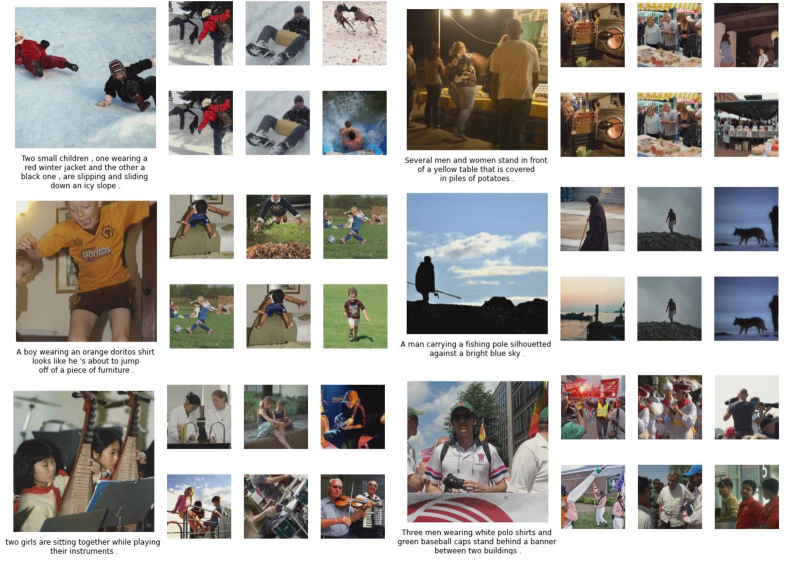
Figure 8: Retrieved images by original image embedding and mixed embedding on Flickr30k.

C.2 Additional Results on Uni-modal Classification

This section provides results of 16-shot uni-modal classification on four new datasets (EuroSAT [99], FGVC Aircraft [100], UCF101 [101], Stanford Cars [102]) with two different models (CLIP ViT-B/16 and CyCLIP [33] ResNet50) that are lacking in the main paper. We perform fine-tuning of them from their official checkpoint relase with the same hyperparameter sweep range described in A of Supplementary. In Table 11, our $m^{2}$-Mix brings consistent performance gain across all datasets and models with some significant boosting on the FGVC Aircraft and Stanford Cars datasets. Thus, $m^{2}$-Mix is a general approach that can enhance the representation learning on various settings.

Table 11: Few-shot classification results with CLIP-VIT-B/16 and CyCLIP-RN50 models. We follow the same few-shot evaluation protocol and contrastive learning strategy with Sec 5.4. in our manuscript. $m^{2}$-Mix consistently outperforms the baseline methods across four datasets. Especially, on Aircraft, $m^{2}$-Mix achieves 8.5% and 4.7% gain over FT in CLIP and CyCLIP, respectively, and 5.2% gain over FT in CyCLIP on Cars.

Model	Method	Dataset
		EuroSAT	Aircraft	UCF101	Cars
CLIP (ViT-B/16)	ZS	48.41	24.81	67.46	65.33
	FT	94.03	60.61	86.36	88.58
	FT w/ $m^{2}$-Mix	94.33	69.07	86.94	90.36
CyCLIP (RN50)	FT	84.98	48.19	67.25	67.02
	FT w/ $m^{2}$-Mix	85.22	52.96	68.97	72.22

Next, in Figure 9 and 10, we perform ablation on the parameter $\alpha$ of Beta distribution, which stochastically determines the mixing ratio between two modalities. Red and Blue colors denote a constant parameter and a linear scheduling parameter, respectively. We see that lower value $\alpha$ (U-shaped Beta distribution) generally achieves better performance than larger values (uniform or reversed U-shaped) on the two classification datasets.

Linear scheduling of Beta parameters drives promising results in some cases, e.g., $1.0->0.1$ and $2.0->0.1$ in Stanford Cars. It seems crucial to enforce that the shape of Beta distribution ends up with a U-shape for the success of scheduling variants. That is, the small-to-many mixing fashion is better than that of half-to-half for the geodesic multi-modal Mixup on classification.

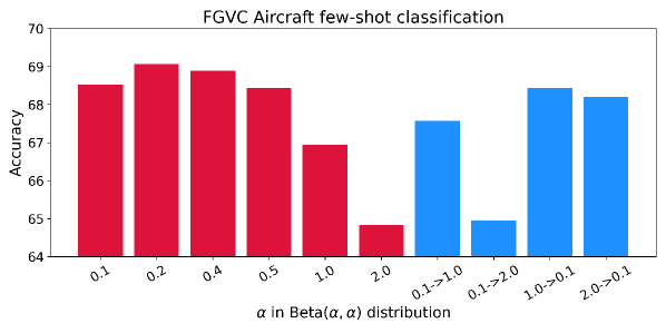
Figure 9: Few-shot classification results on FGVC Aircraft dataset. We varied the parameter of Beta distribution, constant (red) or scheduled (blue), to simulate diverse situations of mixed samples. It always achieves better performance than FT (60.61), even under varying parameters.

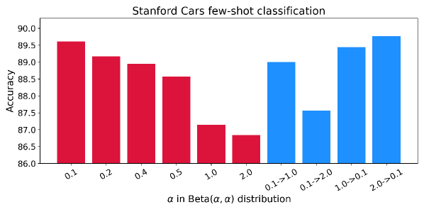
Figure 10: Few-shot classification results on Stanford Cars dataset. We varied the parameter of Beta distribution, constant (red) or scheduled (blue), to simulate diverse situations of mixed samples. It generally achieves better performance than FT (88.58), even under varying parameters.

C.3 Additional Results on Multi-modal Classification

In addition to classification accuracy (in the main paper), we additionally present the F1-score (in Tab. 12) for diagnosis on classification results. While GMC with $m^{2}$-Mix is outperformed by GMC in two of three single-modality cases, it shows superior results on two-modality-given cases based on explicit enforcement of bi-to-joint alignment during training.

Table 12: Classification F1-score on CMU-MOSEI under complete and partial observation modalities. We report the mean performance and standard deviation of five runs.

Method Test-time Observed Modalities Full(T+V+A) T V A T+V T+A V+A MulT 0.8056$\pm$0.004 0.6909$\pm$0.051 0.5678$\pm$0.107 0.6021$\pm$0.151 0.6453$\pm$0.096 0.6657$\pm$0.097 0.5922$\pm$0.111 GMC 0.8054$\pm$0.001 0.7846$\pm$0.006 0.6548$\pm$0.008 0.6910$\pm$0.008 0.7747$\pm$0.009 0.7810$\pm$0.003 0.6978$\pm$0.004 GMC+$m^{2}$-Mix 0.8086$\pm$0.001 0.7882$\pm$0.005 0.6522$\pm$0.006 0.6875$\pm$0.0080 0.7814$\pm$0.004 0.7840$\pm$0.004 0.6988$\pm$0.003

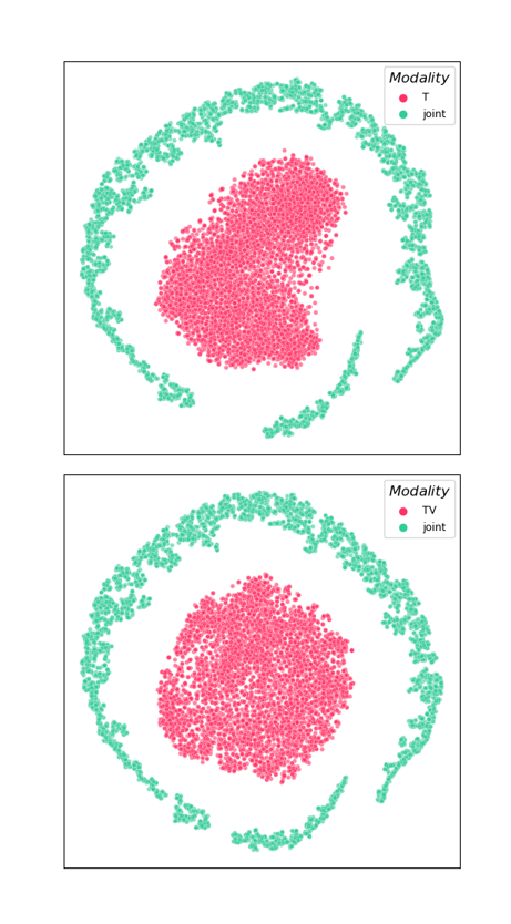
(a) MulT

(b) GMC

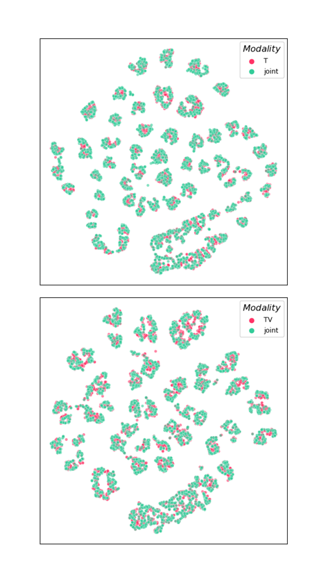
(c) GMC+$m^{2}$-Mix

Figure 11: t-SNE [85] for CMU-MOSEI, which has textual (T), visual (V), and audio (A) modalities. Top row represents when the only textual (T) information is given, and the bottom row corresponds to when the textual (T) and visual (V) information are given. The pink and green color denotes the embedding of partial and joint modality.

Fig. 11 shows the embedding t-SNE of each method given one (top row) or two (bottom row) modalities in test-time. Compared with MulT, GMC strongly aligns the embedding of partial and joint modality based on its explicit enforcement, and the alignment is further enhanced by the aid of $m^{2}$-Mix, which results in superior performance (in Tab. 7 of the main paper, Tab. 12 of supplementary) when only partial (missing modality) information is given during test-time. These results justify the use of our $m^{2}$-Mix for robust multi-modal representation learning under missing modality scenarios.

C.4 Effect of $m^{2}\text{-Mix}$ on Contrastive Learning

This section provides a more detailed analysis of $m^{2}$-Mix. Specifically, we present (i) the proportion of negative pairs (original and mixed) that exceed the similarity between that of positive pairs (See Fig. 12 - 15), and (ii) the similarity comparison between positive and original negative pairs with and without $L_{m^{2}\text{-Mix}}$ (See Fig. 16 and 17). All results are from cross-modal retrieval with CLIP ViT-B/32 on Flickr30k and MS COCO.

Fig. 12 - 15 show the average proportion of in-batch negative pairs’ similarities that exceeds the similarities of positive pairs during training iterations (dataset: MS COCO - Fig. 12 and 13, Flickr30k - Fig. 14 and 15, similarity computation: $I$-to-mixed - Fig. 12 and 14, $T$-to-mixed - Fig. 13 and 15).

Figure 12: Hard negative proportion by $I$-to-mixed samples’ similarities on MS COCO.

Figure 13: Hard negative proportion by $T$-to-mixed samples’ similarities on MS COCO.

Figure 14: Hard negative proportion by $I$-to-mixed samples’ similarities on Flickr30k.

Figure 15: Hard negative proportion by $T$-to-mixed samples’ similarities on Flickr30k.

When we train our model with learning objective $L_{\text{CLIP}}+L_{m^{2}\text{-Mix}}$, the similarities of negative pairs by our $m^{2}$-Mix significantly higher than not only original negatives’ similarities but also positive similarities. Especially in the early training iterations, the proportion is about one in Fig 12 - 14, i.e., almost all of the in-batch negative pairs have higher similarities than positive ones. These results advocate our assumption in proof of Proposition 4.2. (of the main paper and Proposition 1 of this supplementary). That is, $m^{2}$-Mix-generated negative pairs empirically have higher similarities than positive ones. Even though such a hard negative proportion is decaying as the training progresses (by pursuing alignment), it still has not vanished to zero, i.e., uniformity is encouraged until the end of training while the magnitude is getting weaker.

Next, in Fig. 16 left and 17 left, we present the in-batch averaged pairwise similarity from normal negative pairs and positive pairs, which contribute to the computation of $L_{\text{CLIP}}$. We evaluate the similarities under two scenarios whether our $L_{m^{2}\text{-Mix}}$ is adopted together with $L_{\text{CLIP}}$ (dashed line) or not (solid line). Among negative pair similarities, we only consider that of the top-1 hardest negative pair that is related to the definition of relative alignment (Eq. 2 in the main paper) and contrastive loss in an asymptotic scheme (Theorem 4.2. in the main paper).

As we can see in both Fig. 16 and 17, the top-1 original negatives’ similarities and positives’ similarities are increased by using $m^{2}$-Mix, even though the hard negatives generated by $m^{2}$-Mix are not explicitly consumed in $L_{\text{CLIP}}$. Consequently, the alignment is strongly enhanced (left side of Fig. 16 and 17). The results can be summarized as follows: (1) Whether $L_{m^{2}\text{-Mix}}$ is used or not, the similarities between positive pairs are larger than that of original negative pairs during the whole training time. (2) However, if $L_{m^{2}\text{-Mix}}$ is used with $L_{\text{CLIP}}$, the top-1 negative similarities are increased. (3) As a result, the similarities between positive pairs are increased to decrease the contrastive loss $L_{\text{CLIP}}$ (which converges asymptotically to triplet loss).

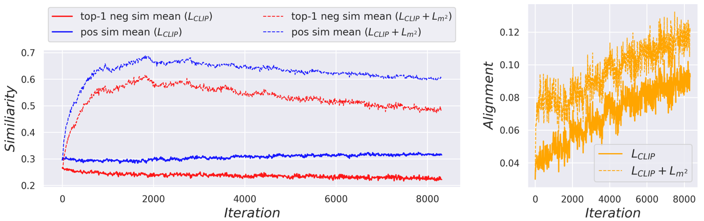
Figure 16: In-batch averaged pairwise similarity and alignment comparison over training iterations with and without $m^{2}$-Mix on MS COCO. (Left) similarities of original negative pairs (top-1 highest) and that of positive pairs. (Right) alignment comparison.

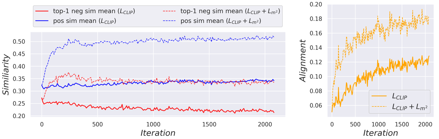
Figure 17: In-batch averaged pairwise similarity and alignment comparison over training iterations with and without $m^{2}$-Mix on Flickr30k. (Left) similarities of original negative pairs (top-1 highest) and that of positive pairs. (Right) alignment comparison.

These empirical results imply that our $L_{m^{2}\text{-Mix}}$ implicitly helps the alignment in $L_{\text{CLIP}}$, and by minimizing $L_{\text{CLIP}}+L_{m^{2}\text{-Mix}}$, we can deal with both alignment and uniformity better (Proposition 4.2. of main paper).

Appendix D Proof

Theorem D.1 (Hardness of $m^{2}$-Mixed samples).

Let’s assume that two random variables $x_{1}$ and $x_{2}$ follow the $M_{d}(\mu_{1},\kappa)$ and $M_{d}(\mu_{2},\kappa)$, von Mises–Fisher distribution with mean direction $\mu_{1},\mu_{2}$ and concentration parameter $\kappa$ in $\mathbb{R}^{d}$, respectively. Let $\widetilde{x}=x_{1}+x_{2}$ and $d=2$. Then, $D_{KL}(p(x_{1})||p(\widetilde{x}))\leq D_{KL}(p(x_{1})||p(x_{2}))$ for sufficiently large $\kappa$.

Proof of Theorem D.1.

Let $M_{d}(\mu,\kappa)=C_{d}(\kappa)\exp(\kappa\mu^{T}x)$, where $C_{d}(\kappa)=\frac{\kappa^{d/2-1}}{(2\pi)^{(d/2)}I_{d/2-1}(\kappa)}$. Let $x_{1}\sim M_{2}(\mu_{1},\kappa)$ and $x_{2}\sim M_{2}(\mu_{1},\kappa)$, and $I$ denotes the modified Bessel function. From [103], $\widetilde{x}\sim M_{2}(\widetilde{\mu},\widetilde{\kappa})$ where $\widetilde{\mu}=\mu_{1}+\mu_{2}$ and $\widetilde{\kappa}=A^{-1}(A(\kappa)A(\kappa))$, approximately, where $A(\kappa)=\frac{I_{1}(\kappa)}{I_{0}(\kappa)}$ and $A^{-1}$ is its inverse. From [104], $D_{KL}(p(x_{1})||p(x_{2}))=\kappa A(\kappa)(1-\text{cos}(\mu_{1}-\mu_{2}))$. Similarly, $D_{KL}(p(x_{1})||p(\widetilde{x}))=\log I_{0}(\widetilde{\kappa})-\log I_{0}(\kappa)+\widetilde{\kappa}A(\widetilde{\kappa})(1-\text{cos}(\mu_{1}-\mu_{2}))$. From [105] and [106], $I_{0}(\kappa)\approx\frac{\exp(\kappa)}{\sqrt{2\pi\kappa}}(1+\frac{1}{8\kappa})\text{ and }I_{1}(\kappa)\approx\frac{\exp(\kappa)}{\sqrt{2\pi\kappa}}(1-\frac{3}{8\kappa})$ for sufficiently large $\kappa$. Therefore, $D_{KL}(p(x_{1})||p(\widetilde{x}))\leq D_{KL}(p(x_{1})||p(x_{2}))$ for sufficiently large $\kappa$. ∎

Proposition D.2 (Limiting behavior of $\mathcal{L}_{\text{CLIP}}$ with $m^{2}$-Mix).

For sufficiently large $M$, as the temperature of contrastive loss $\tau\to 0^{+}$, the $\mathcal{L}_{\text{CLIP}}$ and $\mathcal{L}_{m^{2}\text{-Mix}}$ converge to the triplet loss with zero-margin (i.e., corresponding to negative Alignment) and negative Uniformity, respectively. That is: $\lim_{\tau\to 0^{+}}\mathcal{L}_{\text{CLIP}}+\mathcal{L}_{m^{2}\text{-Mix}}\simeq-(\text{Alignment}+\text{Uniformity})$

Proof of Proposition D.2.

As noted in Section 3., given a training batch $\{x_{i},y_{i}\}_{i=1}^{M}$ of image-text pairs and image and text encoders $f(\cdot;\theta_{1})$ and $g(\cdot;\theta_{2})$, and the $L_{2}$-normalized image-text embeddings are $(I,T)=\{f(x_{i};\theta_{1}),g(y_{i};\theta_{2})\}_{i=1}^{M}$. Then, for $\theta=\{\theta_{1},\theta_{2}\}$ and a scalar $\tau>0$, a standard contrastive loss adopted by CLIP is formulated as:

$$C(I,T;\theta)=\frac{1}{M}\sum_{i=1}^{M}-\log\frac{\exp((I_{i}\cdot T_{i})/\tau)}{\sum_{j=1}^{M}\exp{((I_{i}\cdot T_{j})/\tau})}$$ (6)

Although the actual loss function is constructed by averaging two-way contrastive losses, i.e., $L_{CL}=\frac{1}{2}(C(I,T;\theta)+C(T,I;\theta))$, here, we consider only one-way contrastive loss $C(I,T;\theta)$ for simplicity. It is easily shown the derivation of the other side by changing the order of $I$ and $T$.

During pre-training, the temperature $\tau$ of CLIP converges to 0.01, which is a significantly small value that makes the pair-wise similarities sharp. Thus, it will be reasonable to consider an extreme case: when $\tau\to 0^{+}$. In this case, we can approximate the $C(I,T;\theta)$ as follow:

$$C(I,T;\theta) =\lim_{\tau\to 0^{+}}\frac{1}{M}\sum_{i=1}^{M}-\log\frac{\exp(I_{i}\cdot T_{i}/\tau)}{\sum_{j=1}^{M}\exp{(I_{i}\cdot T_{j}/\tau})}$$ (7)

$$=\lim_{\tau\to 0^{+}}\frac{1}{M}\sum_{i=1}^{M}-(I_{i}\cdot T_{i})/\tau+\log\left[\exp{(I_{i}\cdot T_{i}/\tau)}+\sum_{j\neq i}\exp{(I_{i}\cdot T_{j}/\tau)}\right]$$

$$=\lim_{\tau\to 0^{+}}\frac{1}{M}\sum_{i=1}^{M}\log\left[1+\sum_{j\neq i}\exp{((I_{i}\cdot T_{j})-(I_{i}\cdot T_{i})/\tau)}\right]$$

$$=\lim_{\tau\to 0^{+}}\frac{1}{M}\sum_{i=1}^{M}\log\left[1+\sum_{j\in\mathcal{J}(i,I,T)}\exp{((I_{i}\cdot T_{j})-(I_{i}\cdot T_{i})/\tau)}\right] \mathcal{J}(i,I,T):=\{j|(I_{i}\cdot T_{j})>(I_{i}\cdot T_{i})\}$$ (where )

$$=\lim_{\tau\to 0^{+}}\frac{1}{M}\sum_{i=1}^{M}\frac{1}{\tau}\max\left[\max_{j}(I_{i}\cdot T_{j})-(I_{i}\cdot T_{i}),0\right]$$

$$\simeq\lim_{\tau\to 0^{+}}-\text{Alignment}(I,T;\theta) \max_{j}(I_{i}\cdot T_{j})-(I_{i}\cdot T_{i})>0 M$$ (when and is sufficiently large)

where $\max_{j}(I_{i}\cdot T_{j})$ denotes the maximum similarity among negative pairs. From this derivation, we show that the multi-modal contrastive loss only considers the top-1 hardest negative pairs to positive ones like a triplet loss. As a result, minimizing this loss function is equivalent to maximizing the relative alignment that we newly defined in this paper (in Section 3. Eq. 2 of main paper), e.g., for sufficiently large $M$, $\displaystyle\operatorname*{minimize}_{\theta}\;C(I,T;\theta)\;\equiv\;\operatorname*{maximize}_{\theta}\;\text{Alignment}(I,T;\theta)$. Note that, however, if there are no hard negatives that have higher similarity than positives, the above loss term does not give a meaningful learning signal because the loss already approaches zero. This issue is resolved by $m^{2}$-Mix, which generates hard negatives explicitly.

Next, when we consider the $m^{2}$-Mix-based contrastive loss under same case ($\tau\to 0^{+}$), we can obtain another approximation like below:

$$C_{m^{2}\text{-Mix}}(I,T;\theta) =\lim_{\tau\to 0^{+}}\frac{1}{M}\sum_{i=1}^{M}-\log\frac{\exp(I_{i}\cdot T_{i}/\tau)}{\exp{(I_{i}\cdot T_{i}/\tau)}+\sum_{j\neq i}\exp{(I_{i}\cdot m_{\lambda}(I_{i},T_{j})/\tau})}$$ (8)

$$=\lim_{\tau\to 0^{+}}\frac{1}{M}\sum_{i=1}^{M}-(I_{i}\cdot T_{i})/\tau+\log\left[\exp{(I_{i}\cdot T_{i}/\tau)}+\sum_{j\neq i}\exp{(I_{i}\cdot m_{\lambda}(I_{i},T_{j})/\tau)}\right]$$

$$=\lim_{\tau\to 0^{+}}\frac{1}{M}\sum_{i=1}^{M}\log\left[1+\sum_{j\neq i}\exp{((I_{i}\cdot m_{\lambda}(I_{i},T_{j})-(I_{i}\cdot T_{i}))/\tau)}\right]$$

$$=\lim_{\tau\to 0^{+}}\frac{1}{M}\sum_{i=1}^{M}\log\left[1+\sum_{j\neq i}\exp{(I_{i}\cdot m_{\lambda}(I_{i},T_{j})/\tau)}\right] I_{i}\cdot m_{\lambda}(I_{i},T_{j})>I_{i}\cdot T_{i}\;\text{for all}\;j\neq i$$ (by assuming )

$$=\lim_{\tau\to 0^{+}}\frac{1}{M}\sum_{i=1}^{M}\log\sum_{j\neq i}\exp{(I_{i}\cdot m_{\lambda}(I_{i},T_{j})/\tau)}$$

$$\simeq\lim_{\tau\to 0^{+}}-\text{Uniformity}(I,m_{\lambda}(I_{i},T_{j});\theta) M$$ (for sufficiently large )

Where $m_{\lambda}(\cdot,\cdot)$ is the geodesic Mixup operation with mixing ratio $\lambda$. Based on above Eq. 8, we argue that our $m^{2}$-Mix asymptotically maximizes the uniformity given sufficiently in-batch large samples $M$, i.e., $\displaystyle\operatorname*{minimize}_{\theta}\;C_{m^{2}\text{-Mix}}(I,T;\theta)\;\equiv\;\operatorname*{maximize}_{\theta}\;\text{Uniformity}(I,m_{\lambda}(I_{i},T_{j});\theta)$.

To complete the proof, consider the two-side contrastive losses $L_{\text{CLIP}}=\frac{1}{2}(C(I,T;\theta)+C(T,I;\theta))$ and $L_{m^{2}\text{-Mix}}=\frac{1}{2}(C_{m^{2}\text{-Mix}}(I,T;\theta)+C_{m^{2}\text{-Mix}}(T,I;\theta))$. Then, by minimizing the combination of the standard contrastive loss $L_{\text{CLIP}}(\theta)$ (Eq. 7) and $L_{m^{2}\text{-Mix}}(\theta)$ (Eq. 8), we can approximately maximize both Alignment and Uniformity. ∎

Appendix E Limitation

While our method showcases its versatility on diverse downstream tasks, it induces computational overhead to some extent. In this work, we observed that uniformity and alignment (our modified formulation) are both somewhat correlated with downstream performance, so we argued that uniformity and alignment are crucial in multi-modal representation learning as well as uni-modal representation learning [25, 26]. However, those two metrics are not absolute ones for various situations, e.g., when the modality-specific unique information is important, the higher uniformity and alignment can cause the loss of modality-specific information. The increased computational cost for additional contrastive loss terms is another limitation.

References

- [1] Rishi Bommasani, Drew A Hudson, Ehsan Adeli, Russ Altman, Simran Arora, Sydney von Arx, Michael S Bernstein, Jeannette Bohg, Antoine Bosselut, Emma Brunskill, et al. On the opportunities and risks of foundation models. arXiv preprint arXiv:2108.07258, 2021.
- [2] Andrew Jaegle, Felix Gimeno, Andy Brock, Oriol Vinyals, Andrew Zisserman, and Joao Carreira. Perceiver: General perception with iterative attention. In International conference on machine learning, pages 4651–4664. PMLR, 2021.
- [3] Andrew Jaegle, Sebastian Borgeaud, Jean-Baptiste Alayrac, Carl Doersch, Catalin Ionescu, David Ding, Skanda Koppula, Daniel Zoran, Andrew Brock, Evan Shelhamer, Olivier J Henaff, Matthew Botvinick, Andrew Zisserman, Oriol Vinyals, and Joao Carreira. Perceiver IO: A general architecture for structured inputs & outputs. In International Conference on Learning Representations, 2022.
- [4] Xizhou Zhu, Jinguo Zhu, Hao Li, Xiaoshi Wu, Hongsheng Li, Xiaohua Wang, and Jifeng Dai. Uni-perceiver: Pre-training unified architecture for generic perception for zero-shot and few-shot tasks. In Proceedings of the IEEE/CVF Conference on Computer Vision and Pattern Recognition, pages 16804–16815, 2022.
- [5] Christoph Schuhmann, Romain Beaumont, Richard Vencu, Cade W Gordon, Ross Wightman, Mehdi Cherti, Theo Coombes, Aarush Katta, Clayton Mullis, Mitchell Wortsman, et al. Laion-5b: An open large-scale dataset for training next generation image-text models. In Thirty-sixth Conference on Neural Information Processing Systems Datasets and Benchmarks Track, 2022.
- [6] Linxi Fan, Guanzhi Wang, Yunfan Jiang, Ajay Mandlekar, Yuncong Yang, Haoyi Zhu, Andrew Tang, De-An Huang, Yuke Zhu, and Anima Anandkumar. Minedojo: Building open-ended embodied agents with internet-scale knowledge. In Thirty-sixth Conference on Neural Information Processing Systems Datasets and Benchmarks Track, 2022.
- [7] Samir Yitzhak Gadre, Gabriel Ilharco, Alex Fang, Jonathan Hayase, Georgios Smyrnis, Thao Nguyen, Ryan Marten, Mitchell Wortsman, Dhruba Ghosh, Jieyu Zhang, et al. Datacomp: In search of the next generation of multimodal datasets. arXiv preprint arXiv:2304.14108, 2023.
- [8] Hong Liu, Jeff Z. HaoChen, Adrien Gaidon, and Tengyu Ma. Self-supervised learning is more robust to dataset imbalance. In International Conference on Learning Representations, 2022.
- [9] Jeff Z. HaoChen, Colin Wei, Ananya Kumar, and Tengyu Ma. Beyond separability: Analyzing the linear transferability of contrastive representations to related subpopulations. In Alice H. Oh, Alekh Agarwal, Danielle Belgrave, and Kyunghyun Cho, editors, Advances in Neural Information Processing Systems, 2022.
- [10] Mitchell Wortsman, Gabriel Ilharco, Mike Li, Jong Wook Kim, Hannaneh Hajishirzi, Ali Farhadi, Hongseok Namkoong, and Ludwig Schmidt. Robust fine-tuning of zero-shot models. arXiv preprint arXiv:2109.01903, 2021.
- [11] Ananya Kumar, Aditi Raghunathan, Robbie Jones, Tengyu Ma, and Percy Liang. Fine-tuning can distort pretrained features and underperform out-of-distribution. arXiv preprint arXiv:2202.10054, 2022.
- [12] Polina Kirichenko, Pavel Izmailov, and Andrew Gordon Wilson. Last layer re-training is sufficient for robustness to spurious correlations. In The Eleventh International Conference on Learning Representations, 2023.
- [13] Aaron Van den Oord, Yazhe Li, and Oriol Vinyals. Representation learning with contrastive predictive coding. arXiv e-prints, pages arXiv–1807, 2018.
- [14] Kaiming He, Haoqi Fan, Yuxin Wu, Saining Xie, and Ross Girshick. Momentum contrast for unsupervised visual representation learning. arXiv preprint arXiv:1911.05722, 2019.
- [15] Ting Chen, Simon Kornblith, Mohammad Norouzi, and Geoffrey Hinton. A simple framework for contrastive learning of visual representations. In International conference on machine learning, pages 1597–1607. PMLR, 2020.
- [16] Yuning You, Tianlong Chen, Yongduo Sui, Ting Chen, Zhangyang Wang, and Yang Shen. Graph contrastive learning with augmentations. In H. Larochelle, M. Ranzato, R. Hadsell, M.F. Balcan, and H. Lin, editors, Advances in Neural Information Processing Systems, volume 33, pages 5812–5823. Curran Associates, Inc., 2020.
- [17] Tianyu Gao, Xingcheng Yao, and Danqi Chen. SimCSE: Simple contrastive learning of sentence embeddings. In Empirical Methods in Natural Language Processing (EMNLP), 2021.
- [18] Gowthami Somepalli, Avi Schwarzschild, Micah Goldblum, C Bayan Bruss, and Tom Goldstein. Saint: Improved neural networks for tabular data via row attention and contrastive pre-training. In NeurIPS 2022 First Table Representation Workshop, 2022.
- [19] Alec Radford, Jong Wook Kim, Chris Hallacy, Aditya Ramesh, Gabriel Goh, Sandhini Agarwal, Girish Sastry, Amanda Askell, Pamela Mishkin, Jack Clark, et al. Learning transferable visual models from natural language supervision. In International Conference on Machine Learning, pages 8748–8763. PMLR, 2021.
- [20] Zhecan Wang, Noel Codella, Yen-Chun Chen, Luowei Zhou, Jianwei Yang, Xiyang Dai, Bin Xiao, Haoxuan You, Shih-Fu Chang, and Lu Yuan. Clip-td: Clip targeted distillation for vision-language tasks. arXiv preprint arXiv:2201.05729, 2022.
- [21] Shan Ning, Longtian Qiu, Yongfei Liu, and Xuming He. Hoiclip: Efficient knowledge transfer for hoi detection with vision-language models. arXiv preprint arXiv:2303.15786, 2023.
- [22] Sarah Pratt, Ian Covert, Rosanne Liu, and Ali Farhadi. What does a platypus look like? generating customized prompts for zero-shot image classification. In Proceedings of the IEEE/CVF International Conference on Computer Vision (ICCV), pages 15691–15701, October 2023.
- [23] Ziqin Zhou, Yinjie Lei, Bowen Zhang, Lingqiao Liu, and Yifan Liu. Zegclip: Towards adapting clip for zero-shot semantic segmentation. In Proceedings of the IEEE/CVF Conference on Computer Vision and Pattern Recognition, pages 11175–11185, 2023.
- [24] Yao Lu, Jukka Corander, and Zhirong Yang. Doubly stochastic neighbor embedding on spheres. Pattern Recognition Letters, 128:100–106, 2019.
- [25] Tongzhou Wang and Phillip Isola. Understanding contrastive representation learning through alignment and uniformity on the hypersphere. In International Conference on Machine Learning, pages 9929–9939. PMLR, 2020.
- [26] Feng Wang and Huaping Liu. Understanding the behaviour of contrastive loss. In Proceedings of the IEEE/CVF conference on computer vision and pattern recognition, pages 2495–2504, 2021.
- [27] Weixin Liang, Yuhui Zhang, Yongchan Kwon, Serena Yeung, and James Zou. Mind the gap: Understanding the modality gap in multi-modal contrastive representation learning. In Alice H. Oh, Alekh Agarwal, Danielle Belgrave, and Kyunghyun Cho, editors, Advances in Neural Information Processing Systems, 2022.
- [28] Joshua David Robinson, Ching-Yao Chuang, Suvrit Sra, and Stefanie Jegelka. Contrastive learning with hard negative samples. In International Conference on Learning Representations, 2021.
- [29] Yannis Kalantidis, Mert Bulent Sariyildiz, Noe Pion, Philippe Weinzaepfel, and Diane Larlus. Hard negative mixing for contrastive learning. Advances in Neural Information Processing Systems, 33:21798–21809, 2020.
- [30] Yujia Li, Chenjie Gu, Thomas Dullien, Oriol Vinyals, and Pushmeet Kohli. Graph matching networks for learning the similarity of graph structured objects. In International conference on machine learning, pages 3835–3845. PMLR, 2019.
- [31] Chao Jia, Yinfei Yang, Ye Xia, Yi-Ting Chen, Zarana Parekh, Hieu Pham, Quoc Le, Yun-Hsuan Sung, Zhen Li, and Tom Duerig. Scaling up visual and vision-language representation learning with noisy text supervision. In International Conference on Machine Learning, pages 4904–4916. PMLR, 2021.
- [32] Jiacheng Xu and Greg Durrett. Spherical latent spaces for stable variational autoencoders. In Proceedings of the 2018 Conference on Empirical Methods in Natural Language Processing, pages 4503–4513, 2018.
- [33] Shashank Goel, Hritik Bansal, Sumit Bhatia, Ryan Rossi, Vishwa Vinay, and Aditya Grover. Cyclip: Cyclic contrastive language-image pretraining. Advances in Neural Information Processing Systems, 35:6704–6719, 2022.
- [34] Yannis Kalantidis, Mert Bulent Sariyildiz, Noe Pion, Philippe Weinzaepfel, and Diane Larlus. Hard negative mixing for contrastive learning. In H. Larochelle, M. Ranzato, R. Hadsell, M. F. Balcan, and H. Lin, editors, Advances in Neural Information Processing Systems, volume 33, pages 21798–21809. Curran Associates, Inc., 2020.
- [35] Yifan Zhang, Bryan Hooi, Dapeng Hu, Jian Liang, and Jiashi Feng. Unleashing the power of contrastive self-supervised visual models via contrast-regularized fine-tuning. In A. Beygelzimer, Y. Dauphin, P. Liang, and J. Wortman Vaughan, editors, Advances in Neural Information Processing Systems, 2021.
- [36] Rui Zhu, Bingchen Zhao, Jingen Liu, Zhenglong Sun, and Chang Wen Chen. Improving contrastive learning by visualizing feature transformation. In Proceedings of the IEEE/CVF International Conference on Computer Vision, pages 10306–10315, 2021.
- [37] Hongyi Zhang, Moustapha Cisse, Yann N Dauphin, and David Lopez-Paz. mixup: Beyond empirical risk minimization. In International Conference on Learning Representations, 2018.
- [38] Sunil Thulasidasan, Gopinath Chennupati, Jeff A Bilmes, Tanmoy Bhattacharya, and Sarah Michalak. On mixup training: Improved calibration and predictive uncertainty for deep neural networks. Advances in Neural Information Processing Systems, 32, 2019.
- [39] Zongbo Han, Zhipeng Liang, Fan Yang, Liu Liu, Lanqing Li, Yatao Bian, Peilin Zhao, Bingzhe Wu, Changqing Zhang, and Jianhua Yao. UMIX: Improving importance weighting for subpopulation shift via uncertainty-aware mixup. In Alice H. Oh, Alekh Agarwal, Danielle Belgrave, and Kyunghyun Cho, editors, Advances in Neural Information Processing Systems, 2022.
- [40] Zongbo Han, Zhipeng Liang, Fan Yang, Liu Liu, Lanqing Li, Yatao Bian, Peilin Zhao, Qinghua Hu, Bingzhe Wu, Changqing Zhang, et al. Reweighted mixup for subpopulation shift. arXiv preprint arXiv:2304.04148, 2023.
- [41] Vikas Verma, Alex Lamb, Christopher Beckham, Amir Najafi, Ioannis Mitliagkas, David Lopez-Paz, and Yoshua Bengio. Manifold mixup: Better representations by interpolating hidden states. In International Conference on Machine Learning, pages 6438–6447. PMLR, 2019.
- [42] Sangdoo Yun, Dongyoon Han, Seong Joon Oh, Sanghyuk Chun, Junsuk Choe, and Youngjoon Yoo. Cutmix: Regularization strategy to train strong classifiers with localizable features. In Proceedings of the IEEE/CVF international conference on computer vision, pages 6023–6032, 2019.
- [43] Yoon-Yeong Kim, Kyungwoo Song, JoonHo Jang, and Il-chul Moon. Lada: Look-ahead data acquisition via augmentation for deep active learning. Advances in Neural Information Processing Systems, 34, 2021.
- [44] Jang-Hyun Kim, Wonho Choo, and Hyun Oh Song. Puzzle mix: Exploiting saliency and local statistics for optimal mixup. In International Conference on Machine Learning, pages 5275–5285. PMLR, 2020.
- [45] Hongyu Guo. Nonlinear mixup: Out-of-manifold data augmentation for text classification. In Proceedings of the AAAI Conference on Artificial Intelligence, volume 34, pages 4044–4051, 2020.
- [46] Soyoung Yoon, Gyuwan Kim, and Kyumin Park. Ssmix: Saliency-based span mixup for text classification. In Findings of the Association for Computational Linguistics: ACL-IJCNLP 2021, pages 3225–3234, 2021.
- [47] Huiyun Yang, Huadong Chen, Hao Zhou, and Lei Li. Enhancing cross-lingual transfer by manifold mixup. arXiv preprint arXiv:2205.04182, 2022.
- [48] Yiwei Wang, Wei Wang, Yuxuan Liang, Yujun Cai, and Bryan Hooi. Mixup for node and graph classification. In Proceedings of the Web Conference 2021, pages 3663–3674, 2021.
- [49] Vikas Verma, Meng Qu, Kenji Kawaguchi, Alex Lamb, Yoshua Bengio, Juho Kannala, and Jian Tang. Graphmix: Improved training of gnns for semi-supervised learning. In Proceedings of the AAAI Conference on Artificial Intelligence, 2021.
- [50] Kibok Lee, Yian Zhu, Kihyuk Sohn, Chun-Liang Li, Jinwoo Shin, and Honglak Lee. i-mix: A domain-agnostic strategy for contrastive representation learning. In ICLR, 2021.
- [51] Zhiqiang Shen, Zechun Liu, Zhuang Liu, Marios Savvides, Trevor Darrell, and Eric Xing. Un-mix: Rethinking image mixtures for unsupervised visual representation learning. 2022.
- [52] Qingkai Fang, Rong Ye, Lei Li, Yang Feng, and Mingxuan Wang. Stemm: Self-learning with speech-text manifold mixup for speech translation. arXiv preprint arXiv:2203.10426, 2022.
- [53] Xize Cheng, Tao Jin, Rongjie Huang, Linjun Li, Wang Lin, Zehan Wang, Ye Wang, Huadai Liu, Aoxiong Yin, and Zhou Zhao. Mixspeech: Cross-modality self-learning with audio-visual stream mixup for visual speech translation and recognition. In Proceedings of the IEEE/CVF International Conference on Computer Vision, pages 15735–15745, 2023.
- [54] Alexei Baevski, Wei-Ning Hsu, Qiantong Xu, Arun Babu, Jiatao Gu, and Michael Auli. Data2vec: A general framework for self-supervised learning in speech, vision and language. arXiv preprint arXiv:2202.03555, 2022.
- [55] Hao Li, Jinguo Zhu, Xiaohu Jiang, Xizhou Zhu, Hongsheng Li, Chun Yuan, Xiaohua Wang, Yu Qiao, Xiaogang Wang, Wenhai Wang, et al. Uni-perceiver v2: A generalist model for large-scale vision and vision-language tasks. In Proceedings of the IEEE/CVF Conference on Computer Vision and Pattern Recognition, pages 2691–2700, 2023.
- [56] Jinyu Yang, Jiali Duan, Son Tran, Yi Xu, Sampath Chanda, Liqun Chen, Belinda Zeng, Trishul Chilimbi, and Junzhou Huang. Vision-language pre-training with triple contrastive learning. In Proceedings of the IEEE/CVF Conference on Computer Vision and Pattern Recognition, pages 15671–15680, 2022.
- [57] Amanpreet Singh, Ronghang Hu, Vedanuj Goswami, Guillaume Couairon, Wojciech Galuba, Marcus Rohrbach, and Douwe Kiela. Flava: A foundational language and vision alignment model. In Proceedings of the IEEE/CVF Conference on Computer Vision and Pattern Recognition, pages 15638–15650, 2022.
- [58] Huaishao Luo, Lei Ji, Ming Zhong, Yang Chen, Wen Lei, Nan Duan, and Tianrui Li. Clip4clip: An empirical study of clip for end to end video clip retrieval. arXiv preprint arXiv:2104.08860, 2021.
- [59] Han Fang, Pengfei Xiong, Luhui Xu, and Yu Chen. Clip2video: Mastering video-text retrieval via image clip. arXiv preprint arXiv:2106.11097, 2021.
- [60] Xiuye Gu, Tsung-Yi Lin, Weicheng Kuo, and Yin Cui. Zero-shot detection via vision and language knowledge distillation. CoRR, abs/2104.13921, 2021.
- [61] Gwanghyun Kim and Jong Chul Ye. Diffusionclip: Text-guided image manipulation using diffusion models. CoRR, abs/2110.02711, 2021.
- [62] Kaiyang Zhou, Jingkang Yang, Chen Change Loy, and Ziwei Liu. Learning to prompt for vision-language models. International Journal of Computer Vision, 130(9):2337–2348, 2022.
- [63] Renrui Zhang, Rongyao Fang, Wei Zhang, Peng Gao, Kunchang Li, Jifeng Dai, Yu Qiao, and Hongsheng Li. Tip-adapter: Training-free clip-adapter for better vision-language modeling. arXiv preprint arXiv:2111.03930, 2021.
- [64] Muhammad Uzair Khattak, Hanoona Rasheed, Muhammad Maaz, Salman Khan, and Fahad Shahbaz Khan. Maple: Multi-modal prompt learning. arXiv preprint arXiv:2210.03117, 2022.
- [65] Yassine Ouali, Adrian Bulat, Brais Martinez, and Georgios Tzimiropoulos. Black box few-shot adaptation for vision-language models. arXiv preprint arXiv:2304.01752, 2023.
- [66] Sachin Goyal, Ananya Kumar, Sankalp Garg, Zico Kolter, and Aditi Raghunathan. Finetune like you pretrain: Improved finetuning of zero-shot vision models. 2023.
- [67] Bryan A Plummer, Liwei Wang, Chris M Cervantes, Juan C Caicedo, Julia Hockenmaier, and Svetlana Lazebnik. Flickr30k entities: Collecting region-to-phrase correspondences for richer image-to-sentence models. In Proceedings of the IEEE international conference on computer vision, pages 2641–2649, 2015.
- [68] Florian Schroff, Dmitry Kalenichenko, and James Philbin. Facenet: A unified embedding for face recognition and clustering. In Proceedings of the IEEE conference on computer vision and pattern recognition, pages 815–823, 2015.
- [69] Weiyang Liu, Yandong Wen, Zhiding Yu, Ming Li, Bhiksha Raj, and Le Song. Sphereface: Deep hypersphere embedding for face recognition. In Proceedings of the IEEE conference on computer vision and pattern recognition, pages 212–220, 2017.
- [70] Tsung-Yi Lin, Michael Maire, Serge Belongie, James Hays, Pietro Perona, Deva Ramanan, Piotr Dollár, and C Lawrence Zitnick. Microsoft coco: Common objects in context. In European conference on computer vision, pages 740–755. Springer, 2014.
- [71] Chuan Guo, Geoff Pleiss, Yu Sun, and Kilian Q Weinberger. On calibration of modern neural networks. In International Conference on Machine Learning, pages 1321–1330. PMLR, 2017.
- [72] Xiaohua Zhai, Xiao Wang, Basil Mustafa, Andreas Steiner, Daniel Keysers, Alexander Kolesnikov, and Lucas Beyer. Lit: Zero-shot transfer with locked-image text tuning. In Proceedings of the IEEE/CVF Conference on Computer Vision and Pattern Recognition (CVPR), pages 18123–18133, June 2022.
- [73] Jacob Devlin Ming-Wei Chang Kenton and Lee Kristina Toutanova. Bert: Pre-training of deep bidirectional transformers for language understanding. In Proceedings of NAACL-HLT, pages 4171–4186, 2019.
- [74] Kaiming He, Xiangyu Zhang, Shaoqing Ren, and Jian Sun. Deep residual learning for image recognition. In Proceedings of the IEEE conference on computer vision and pattern recognition, pages 770–778, 2016.
- [75] Omkar M Parkhi, Andrea Vedaldi, Andrew Zisserman, and C. V. Jawahar. Cats and dogs. In 2012 IEEE Conference on Computer Vision and Pattern Recognition, pages 3498–3505, 2012.
- [76] Yuval Netzer, Tao Wang, Adam Coates, Alessandro Bissacco, Bo Wu, and Andrew Y. Ng. Reading digits in natural images with unsupervised feature learning. In NIPS Workshop on Deep Learning and Unsupervised Feature Learning 2011, 2011.
- [77] Justin Johnson, Bharath Hariharan, Laurens Van Der Maaten, Li Fei-Fei, C Lawrence Zitnick, and Ross Girshick. Clevr: A diagnostic dataset for compositional language and elementary visual reasoning. In Proceedings of the IEEE conference on computer vision and pattern recognition, pages 2901–2910, 2017.
- [78] Benjamin Recht, Rebecca Roelofs, Ludwig Schmidt, and Vaishaal Shankar. Do imagenet classifiers generalize to imagenet? In International conference on machine learning, pages 5389–5400. PMLR, 2019.
- [79] Dan Hendrycks, Kevin Zhao, Steven Basart, Jacob Steinhardt, and Dawn Song. Natural adversarial examples. In Proceedings of the IEEE/CVF Conference on Computer Vision and Pattern Recognition, pages 15262–15271, 2021.
- [80] Dan Hendrycks, Steven Basart, Norman Mu, Saurav Kadavath, Frank Wang, Evan Dorundo, Rahul Desai, Tyler Zhu, Samyak Parajuli, Mike Guo, et al. The many faces of robustness: A critical analysis of out-of-distribution generalization. In Proceedings of the IEEE/CVF International Conference on Computer Vision, pages 8340–8349, 2021.
- [81] Haohan Wang, Songwei Ge, Zachary Lipton, and Eric P Xing. Learning robust global representations by penalizing local predictive power. In Advances in Neural Information Processing Systems, pages 10506–10518, 2019.
- [82] Kaiyang Zhou, Jingkang Yang, Chen Change Loy, and Ziwei Liu. Conditional prompt learning for vision-language models. In Proceedings of the IEEE/CVF Conference on Computer Vision and Pattern Recognition, pages 16816–16825, 2022.
- [83] AmirAli Bagher Zadeh, Paul Pu Liang, Soujanya Poria, Erik Cambria, and Louis-Philippe Morency. Multimodal language analysis in the wild: CMU-MOSEI dataset and interpretable dynamic fusion graph. In Proceedings of the 56th Annual Meeting of the Association for Computational Linguistics (Volume 1: Long Papers), pages 2236–2246, Melbourne, Australia, July 2018. Association for Computational Linguistics.
- [84] Petra Poklukar, Miguel Vasco, Hang Yin, Francisco S Melo, Ana Paiva, and Danica Kragic. Gmc–geometric multimodal contrastive representation learning. arXiv preprint arXiv:2202.03390, 2022.
- [85] Laurens Van der Maaten and Geoffrey Hinton. Visualizing data using t-sne. Journal of machine learning research, 9(11), 2008.
- [86] Yao-Hung Hubert Tsai, Shaojie Bai, Paul Pu Liang, J Zico Kolter, Louis-Philippe Morency, and Ruslan Salakhutdinov. Multimodal transformer for unaligned multimodal language sequences. In Proceedings of the conference. Association for Computational Linguistics. Meeting, volume 2019, page 6558. NIH Public Access, 2019.
- [87] Kawin Ethayarajh, David Duvenaud, and Graeme Hirst. Towards understanding linear word analogies. arXiv preprint arXiv:1810.04882, 2018.
- [88] Guillaume Couairon, Matthieu Cord, Matthijs Douze, and Holger Schwenk. Embedding arithmetic for text-driven image transformation. arXiv preprint arXiv:2112.03162, 2021.
- [89] Yuheng Li, Haotian Liu, Qingyang Wu, Fangzhou Mu, Jianwei Yang, Jianfeng Gao, Chunyuan Li, and Yong Jae Lee. Gligen: Open-set grounded text-to-image generation. arXiv preprint arXiv:2301.07093, 2023.
- [90] Jiahui Yu, Zirui Wang, Vijay Vasudevan, Legg Yeung, Mojtaba Seyedhosseini, and Yonghui Wu. Coca: Contrastive captioners are image-text foundation models. arXiv preprint arXiv:2205.01917, 2022.
- [91] Xiujun Li, Xi Yin, Chunyuan Li, Pengchuan Zhang, Xiaowei Hu, Lei Zhang, Lijuan Wang, Houdong Hu, Li Dong, Furu Wei, et al. Oscar: Object-semantics aligned pre-training for vision-language tasks. In Computer Vision–ECCV 2020: 16th European Conference, Glasgow, UK, August 23–28, 2020, Proceedings, Part XXX 16, pages 121–137. Springer, 2020.
- [92] Amir Zadeh, Rowan Zellers, Eli Pincus, and Louis-Philippe Morency. Multimodal sentiment intensity analysis in videos: Facial gestures and verbal messages. IEEE Intelligent Systems, 31(6):82–88, 2016.
- [93] Kyunghyun Cho, Bart Van Merriënboer, Caglar Gulcehre, Dzmitry Bahdanau, Fethi Bougares, Holger Schwenk, and Yoshua Bengio. Learning phrase representations using rnn encoder-decoder for statistical machine translation. arXiv preprint arXiv:1406.1078, 2014.
- [94] Kishore Papineni, Salim Roukos, Todd Ward, and Wei-Jing Zhu. Bleu: A method for automatic evaluation of machine translation. In Proceedings of the 40th Annual Meeting on Association for Computational Linguistics, ACL ’02, page 311–318, USA, 2002. Association for Computational Linguistics.
- [95] Satanjeev Banerjee and Alon Lavie. METEOR: An automatic metric for MT evaluation with improved correlation with human judgments. In Proceedings of the ACL Workshop on Intrinsic and Extrinsic Evaluation Measures for Machine Translation and/or Summarization, pages 65–72, Ann Arbor, Michigan, June 2005. Association for Computational Linguistics.
- [96] Chin-Yew Lin. ROUGE: A package for automatic evaluation of summaries. In Text Summarization Branches Out, pages 74–81, Barcelona, Spain, July 2004. Association for Computational Linguistics.
- [97] Ramakrishna Vedantam, C Lawrence Zitnick, and Devi Parikh. Cider: Consensus-based image description evaluation. In Proceedings of the IEEE conference on computer vision and pattern recognition, pages 4566–4575, 2015.
- [98] Peter Anderson, Basura Fernando, Mark Johnson, and Stephen Gould. Spice: Semantic propositional image caption evaluation. In Computer Vision–ECCV 2016: 14th European Conference, Amsterdam, The Netherlands, October 11-14, 2016, Proceedings, Part V 14, pages 382–398. Springer, 2016.
- [99] Patrick Helber, Benjamin Bischke, Andreas Dengel, and Damian Borth. Eurosat: A novel dataset and deep learning benchmark for land use and land cover classification. IEEE Journal of Selected Topics in Applied Earth Observations and Remote Sensing, 12(7):2217–2226, 2019.
- [100] Subhransu Maji, Esa Rahtu, Juho Kannala, Matthew Blaschko, and Andrea Vedaldi. Fine-grained visual classification of aircraft. arXiv preprint arXiv:1306.5151, 2013.
- [101] Khurram Soomro, Amir Roshan Zamir, and Mubarak Shah. Ucf101: A dataset of 101 human actions classes from videos in the wild. arXiv preprint arXiv:1212.0402, 2012.
- [102] Jonathan Krause, Michael Stark, Jia Deng, and Li Fei-Fei. 3d object representations for fine-grained categorization. In 2013 IEEE International Conference on Computer Vision Workshops, pages 554–561, 2013.
- [103] Ivan Marković and Ivan Petrović. Bearing-only tracking with a mixture of von mises distributions. In 2012 IEEE/RSJ International Conference on Intelligent Robots and Systems, pages 707–712. IEEE, 2012.
- [104] S Rao Jammalamadaka, Brian Wainwright, and Qianyu Jin. Functional clustering on a circle using von mises mixtures. Journal of Statistical Theory and Practice, 15(2):1–17, 2021.
- [105] P Martin, J Olivares, and A Sotomayor. Precise analytic approximation for the modified bessel function i 1 (x). Revista mexicana de física, 63(2):130–133, 2017.
- [106] J Olivares, P Martin, and E Valero. A simple approximation for the modified bessel function of zero order i0 (x). In Journal of Physics: Conference Series, volume 1043, page 012003. IOP Publishing, 2018.